
Triggering of Rain-Induced Landslides, with Applications in Southern Italy
by
 , , and
Antonino D’Ippolito
1,
Valeria Lupiano
2,*,
Valeria Rago
2,
Oreste G. Terranova
2 and
Giulio Iovine
2 
1
Department of Civil Engineering, University of Calabria, Rende, 87036 Cosenza, Italy
2
CNR-IRPI, Research Institute for Geo-Hydrological Protection, Rende, 87036 Cosenza, Italy
*
Author to whom correspondence should be addressed.
Water 2023, 15(2), 277; https://doi.org/10.3390/w15020277
Submission received: 21 November 2022
/
Revised: 22 December 2022
/
Accepted: 5 January 2023
/
Published: 9 January 2023
(This article belongs to the Section Hydrogeology)
Abstract
:Landslides cause fatalities, widespread damages and economic losses. Quite frequently, they are triggered by rainfall. Many studies have investigated the relationships between rainfall characteristics and landslide events. This paper reviews the two main approaches, physical and hydrological, for modelling such relationships. In the physical approach, the influence of rainfall on slope stability is commonly analysed in terms of groundwater infiltration, pore pressure changes and balance between shear stresses and resistances, therefore a considerable amount of hydrogeological, morphological and geotechnical data is required. In the hydrological approach, a statistical-probabilistic study of rainfall series and dates of occurrence of slope movements is instead carried out. Both types of methods are briefly presented, with examples from real applications to study cases in Southern Italy. In particular, the recent reactivations of a large rockslide in Northern Calabria have been modelled by means of physical and hydrological approaches. In addition, shallow landslides in Calabria, Campania and Sicily have been modelled by employing hydrological approaches. Strengths and weaknesses of the adopted methods are discussed, together with the causes that may have hindered better results for the considered cases. For the methods illustrated through real application cases, research perspectives are discussed, as well as their possible use in early warning systems.
Keywords:
rainfall; landslide; physical model; hydrological model; threshold; early warning; Southern Italy1. Introduction
Exceptional rainfall—in terms of intensity, duration and amount—can seriously damage the anthropic environment and cause suffering. Rainfall intensity, expressed as total amount over a given time horizon, determines the types of resulting ground effects, such as severe erosion on slopes, shallow/deep landslides and flooding.
In the case of landslides triggered by rains, i.e., those considered in this paper, the “critical duration” of the rainfall event (base time, ) mainly depends on the thickness and permeability of the potentially involved material. Among other relevant controlling factors, such as slope, lithotype and structural characteristics [1], soil moisture conditions at the beginning of the rainfall event, which in turn may be affected by vegetation, antecedent rains, seasonality or even anthropic causes, usually assumes a prominent role in shallow-landslide activation (e.g., [2]), as first pointed out by Campbell [3]. Several authors (e.g., [4,5]) provided examples of shallow-landslide activations occurred after prolonged rainy periods, thus confirming the twofold role of rainfall, in terms of being both a predisposing and triggering factor, and proposed thresholds based on a combination of (i) the rains in the day of mobilisation, and (ii) of those recorded in the antecedent period. More recently, results of flume tests performed by Schilirò et al. [6] confirmed that, depending on initial water content, two alternative triggering mechanisms may develop within a given material, either in relation to the raising of a temporary water table or to the downward advance of the wetting front. Furthermore, as underlined by Fredlund and Rahardjo [7], matric suction can deeply affect the stability conditions of unsaturated soil slopes. Similarly, the sudden collapse of high, steep residual/colluvial slopes in Hong Kong was explained by Brand [8] in terms of sudden annulment of negative neutral pressures, due to severe and short downpours.
Deep rain-induced landslides are generally activated by cumulative rainfall over long periods (weeks/months, but even exceeding a hydrologic year), whereas shallow ones are commonly triggered by short-lasting heavy rains (with from fraction of hours to several days) at the end of a wet period (cf. e.g., [9]). Generally speaking, the infiltration of rain increases pore pressures, which in turn reduce the effective shear resistance of the soil, eventually triggering instability. Stability conditions of slopes are therefore affected by infiltration, which causes transient variations in the dynamics of aquifers [10,11,12].
Relationships between rains and landslides have long been investigated by research groups, with a copious production of models and the significant advancement in knowledge [13,14]. Nevertheless, studies mainly dealt with the definition of rainfall thresholds for single landslides or for specific types of slope movements in a homogeneous geo-environmental context, whereas exhaustive general discussions on the topic are not yet available. In the literature, the relationship between rainfall and landslide occurrence is alternatively modelled by two distinct approaches, i.e., (i) “hydrological” or “empirical” and (ii) “complete” or “physical” (with few examples of coupled methods). In hydrological models, statistical-probabilistic analyses of rainfall series associated to the dates of landslide activation are usually performed (see, among others [14,15,16,17]). In addition to single cases, the statistical approach can also be applied to a set of similar slope movements within a large study area (provided it is homogeneous) at low cost and in a reasonable timeframe. One of the first examples of this method was provided by Zaruba [18]: in his pioneering work, a good correlation between wet periods (characterised in terms of three-year moving averages of cumulated rains) and phases of recrudescence of landslide phenomena in Bohemia was evidenced. Physical models, on the other hand, require a high amount of specific knowledge on the considered sites, related to hydrological, hydro-geological, morphological and geotechnical aspects. In such models, a description of the involved processes, from rainfall to runoff and infiltration and therefore from soil erosion to landslide triggering, must be provided in mathematical terms to simulate slope-stability conditions. Examples of in-depth applications of this method are not numerous and limited to cases in which accurate and detailed observations are available [19]. Overall, the complexity of the involved processes, combined with the great variability of environmental contexts and scarcity/poor quality of data, made this approach hard to progress. Due to the need for large volumes of geological/technical data (and due to their cost), the physical approach is better suited to local studies, in which the value of the elements exposed to risk is particularly relevant. In both the hydrological and physical approaches, the quality (reliability of data) is always an essential issue. Generally, in any landslide data base, the following information should be included with adequate detail: geographical location of the slope movement; time of occurrence; landslide type; effects (damages/injuries); lithological, geo-hydrological and structural characteristics; and rainfall records. Unfortunately, the above information is not always available and is commonly characterised by different accuracy levels; therefore, any attempt of an analysis of the relationships between rainfall and landslide activations is often affected by biases.
Any physical system evolves over time, either due to its own internal dynamics or to external perturbations. Tools (sensors and software) may allow us to continuously monitor its evolution, analyse configuration changes and communicate status conditions to authorities, thus providing support to decisions in case of emergency [20,21]. Commonly, critical conditions are defined, based on “threshold” exceedance for selected parameters. The concept of threshold has been the subject of interest in the scientific community for centuries [22]; it denotes a condition, usually identified by a numerical value or a mathematical law, whose occurrence causes a change in state, [23]. An “event” is commonly a piece of information, extracted from the signals (continuous or discrete) provided by the monitoring network. It is considered instantaneous and dated. The definition of “alarm” derives from the concept of event: it is a discrete indicator, distinguished by level or by type, issued by the monitoring system on the basis of events and aimed at generating human or automatic reactions [20].
As concerns landslide triggering, a threshold can then be considered as a binary classifier of the rain conditions that are likely (or not likely) to result in an activation. Accordingly, a contingency table can be employed to list the four possible outcomes, or contingencies [24,25,26] (cf. Appendix A). Hybrid thresholds (e.g., based on a combination of rainfall and groundwater or suction monitoring data) can also be developed for refining the prediction of landslide activations (e.g., [27]). As a whole, thresholds can be fruitfully employed in the frame of early warning “platforms”, i.e., Decision Support Systems (DSS) specifically developed to support authorities for risk mitigation purposes (cf. e.g., [28]). Among the most recent examples (e.g., [29,30]), the national early warning system for rainfall-induced landslides (SANF-[31]) was implemented by the CNR-IRPI for the National Department of Civil Protection to forecast the occurrence of rainfall-induced landslides in Italy, based on rainfall thresholds, sub-hourly rainfall monitoring at a national network of ca. 2000 rain gauges and quantitative rain forecasts. Twice a day, the system compares measured and forecasted rains against intensity–duration thresholds (cf. next section) and assigns to each node of the mesh a probability of landslide occurrence in the next 24 h, allowing for the identification of places where landslides are mostly expected.
As a rule, empirical models need to be calibrated by using a suitable subsample of available information, and then validated against the remaining set of data. Data selection for calibration can be performed by adopting several approaches (cf. e.g., [32,33]). Furthermore, both physical and empirical models should always be thoroughly analysed to verify their sensitivity with respect to involved parameters (cf. [34]).
In the following sections, a synthetic review of the main modelling approaches is presented, with examples of application to study cases in Southern Italy. Furthermore, pros and cons of the considered methods are briefly discussed and research perspectives suggested.
2. Physical Models
According to Terzaghi [35], instability occurs if the shear stress exceeds a threshold value, i.e., the shear strength . This latter can be expressed by the Mohr–Coulomb failure criterion:
where is the cohesive strength of the soil, the normal stress on the slip plane, the pore pressure and the angle of internal friction. In fact, stability conditions are commonly expressed by means of the safety factor (Fs), expressed as:
Values of > 1 express stability, whereas instability corresponds to < 1 ( = 1 denotes critical conditions of impending failure).
Underground, points located close to the “unstable” sector (i.e., the one first affected by rupture) suffer from increased shear stress, and then a larger zone may progressively be affected by failure (wherever shear stress results in exceeding the strength).
To evaluate stability conditions along a vertical (2D) slope section, and must be known at each location. Such parameters are subject to changes in time and may induce significant changes in the safety factor. For a homogeneous lithology and a constant depth of the slip plane, and firstly depend on soil moisture (and then, on rain infiltration), according to a power–law relationship [36]. The shear and normal stresses depend on (i) the weight of water in the soil, according to a linear law, and (ii) on local slope, according to trigonometric functions.
In physical models, the rain amounts (that contribute to infiltration and pore pressures changes) affect in time the balance between shear stress and resistance (cf. e.g., [37,38,39,40,41,42]). Rainfall-induced failures evolve in time according to the dynamics of suspended water tables [43,44,45,46] or groundwater [12].
In slope-stability analyses, an easily implementable, widely used approach is the LEM (Limit Equilibrium Method). It assumes a rupture surface delimiting the mass to be—simultaneously, at each point along the surface—at the “limit equilibrium” state, corresponding to critical conditions. Despite assuming an ideal soil behaviour schematised as a rigid, perfectly plastic medium, for many practical problems LEM provides acceptable solutions in terms of Safety Factor (see [47] and citations therein). In cases of a more complex geometry, Janbu [48] and Bishop [49] provided approximated methods, whereas Morgenstern and Price [50], Spencer [51] and Sarma [52] proposed rigorous methods.
When slope conditions do not conform to plane strain idealisations, two-dimensional slope analyses can prove inaccurate. In such cases (e.g., when lateral heterogeneities in the geometry of failure mass and slope; anisotropic/heterogeneous properties of underground material; local surcharges applied to the slope), a three-dimensional (3D) approach should be employed (cf. [53]; see also [54]). Since the 1970s, stability analyses in 3D have commonly been performed by means of either the LEM or Finite Element Method (FEM), employing different constitutive models. Nevertheless, most of them are applicable only in specific conditions. In 3D LEM, the direction of slide must be carefully determined, in addition to the global minimum safety factor and corresponding critical failure surface, by using “classic” strategies from the literature (e.g., Bishop [49], Morgenstern-Price [50], Janbu [48], Spencer [51]), suitably adapted. Compared to 2D analyses, the safety factor obtained with 3D methods is generally higher. The FEM does not need to assume either the location/shape of the rupture surface nor the lateral forces on slices [55]. A 3D modelling of the slope stability finds in the FEM approach a very efficient tool even in complex cases, e.g., with loads resulting from pore pressure or seismic actions. FEM techniques make it possible to obtain both the minimum factor of safety and the deformation field at sectors subject to rupture, with associated stress states. For 3D slope stability analyses, they can be more easily executed by means of commercial software (STAB3D–cf. [56]; LEMIX, BLOCK 3, and FESPON–cf. [57]; DEEPCYL–cf. [58]; CLARA 2.31–cf. [59], and [60]; FLAC3D–cf. [61]; Scoops3D-i–cf. [62]). Progress in the 3D modelling of slope stability still has a lot of margin for improvement. For example, aspects related to unsaturated soils and to slope evolution over time still need to be thoroughly investigated.
Among the most recent examples of freeware software for checking the stability of natural and artificial slopes (including reinforcing elements), the release 5.1 of SSAP2010 [63,64] provides a set of original tools to perform in-depth stability checks using only rigorous and innovative methods based on an advanced Limit Equilibrium Method, and innovative search engines to find the critical surfaces associated with the minimum safety factor. SSAP allows to obtain reliable values thanks to a more general approach to LEM (“advanced LEM”, based on a hybrid methodology between LEM and FEM, called qFEM). The software includes a numerical stability control and reliability analysis; groundwater and fluid pressure management module, with perched groundwater and fluids seepage force; the effect of various type of reinforcement structures; and a dynamic analysis by seismic pseudo-static and displacement methods. The model is able to consider the following types of failure criteria for soils and fractured rock mass: Mohr–Coulomb, Tresca, Generalized Hoek–Brown GSI (non-linear) [65,66], Barton-Bandis non-linear JCR [67,68], liquefaction condition [69].
The physical approach is commonly adopted for site-oriented studies, through slope stability analyses that require expensive, detailed information on several physical parameters. However, some examples of studies at a regional scale (especially, concerning shallow landslides) were recently performed, based on simplified schemes.
The SHALSTAB is a steady-state model aimed at identifying the pattern of potential shallow landslides [37,70,71]. Applications to real cases pointed out good performances both in calibration and validation by employing proper sets of real landslide sources. The model allows for the identification of unstable sites and provides an objective procedure for delineating sites of potential instability.
The QDSLaM (Quasi-Dynamic Shallow Landsliding Model) is based on a limit-equilibrium slope-stability model coupled to a hydrogeological model and allows us to calculate the critical rainfall necessary to trigger slope instability at any site in the study area [72]. The model employs a “quasi dynamic” wetness index to forecast the spatial distribution of soil saturation as a consequence of rainfall events of a given duration. In the model, water flow is assumed to infiltrate down to a lower conductivity layer and then propagate according to topographically determined flow paths. According to numerical experiments and field evidence, soil depth variability strongly controls the connectivity of saturated zones at the soil–bedrock interface, thus determining the timing and location of instability.
Lanni et al. [73] proposed the Connectivity Index-Based Shallow Landslide Model (CI-SLAM). Aiming at modelling the local pore pressure in the saturated zone, both the vertical infiltration in unsaturated soil and the lateral flow are taken into account, based on the hydrological connectivity. By employing a scaling model for the rainfall frequency–duration relationship, a shallow-landslide hazard map could be obtained, based on the return period () of the critical rainfall.
Trends over time of rainfall infiltration and slope stability, in a discretised domain, can be simulated by TRIGRS (Transient Rainfall Infiltration and Grid-Based Regional Slope-Stability) analysis [74], in which the infiltration model is based on the linearised solution of Richards’s equation [75]. The program computes transient pore-pressure changes due to rainfall infiltration and makes use of an infinite-slope model to compute the safety factor for each cell. Applications of TRIGRS sound useful for hazard zoning at a regional scale (e.g., [76,77,78,79,80]. Nevertheless, in addition to the lack of a user-friendly interface, it requires extended sets of input data (e.g., slope angle, soil depth) and prolonged computational times.
Ciurleo et al. [81] proposed a method for debris-flow modelling by combining the LEM TRIGRS (for the triggering phase) to the Smoothed Particle Hydrodynamics (SPH) model (for propagation). TRIGRS is employed to define the locations and initial volumes of the landslides, whereas SPH simulates flow propagation in terms of main paths and depositional areas. Information on grain-size distribution and on rheological behaviour of the soil–water mixture is required to run the SPH model. The method enables the obtainment of the debris-flow height and velocity-in-time along the path, which are useful for evaluating the impact force and in designing protective structures.
Troncone et al. [82] recently suggested a method for predicting the occurrence of rain-induced shallow landslides that employs a closed-form solution for pore-pressure changes due to rain infiltration, plus an infinite-slope scheme to calculate the critical value of pore pressure that determines failure conditions. Based on the initial pore pressure at a given depth, and on a hyperbolic threshold (defined in terms of infiltration rate and rainfall duration), the method allows for the determination of if a given rain can lead to slope failure. Triggering conditions are assumed in case the water table generates positive pore-water pressures within the slope, exceeding a critical threshold (that can be evaluated by equalling the safety factor with the unity). Results explicitly depend on slope geometry, pre-existing pore-water pressure and soil properties at local scale. The method is analytical and requires few parameters from laboratory tests. Modelling of rainfall-induced shallow landslides in unsaturated soils was also considered by Troncone et al. [83], with a similar approach.
3. Hydrological Models
Campbell [3] first analysed in quantitative terms the empirical relationships between “antecedent” rain, rainfall intensity and shallow landslides triggered on the hilly slopes of the Santa Monica Mt. (California). He suggested that a total cumulative of ca. 267 mm of rain, recorded during the last days before soil-slip mobilisation, combined with a minimum intensity of ca. 6 mm/h, were necessary to explain the triggering of slope instabilities in the considered study area. Similar results on the relevance of the antecedent predisposing rains and on the timing of the triggering thunderstorm (to be placed at the end of the wet period) were also found by Fenti et al. [84] for the T. Fiorentina in Veneto (northern Italy), among others. Still, among the first studies to address this topic, Govi et al. [85] underlined that “critical” events, expressed in terms of hourly intensity vs. percentage of the mean annual rainfall, depended on seasonality. Similar results were obtained in California by Cannon and Ellen [86]. Cancelli and Nova [87] found a linear, negative relationship between the intensity and duration of critical rains needed to trigger shallow landslides in the Central Alps. Sangrey et al. [88], analysing different types of slope movements in California, stressed that there was not a single critical rainfall event for all the considered cases; as further detailed by Cascini and Versace [9], smaller landslide bodies are, in fact, generally mobilised by shorter and more severe rainfall, and vice versa. Crozier [89], starting from Owen’s [90] findings, discussed the relevance of average soil moisture and slope aspect in determining higher rainfall thresholds for shady/wetter locations with respect to sunny/drier ones in New Zealand.
In hydrological models, a critical threshold for landslide triggering can be defined within homogeneous territorial contexts (e.g., in lithological, pedological, geomorphological terms) by considering specific types of instability, based on available rain data and on information concerning past activations [91,92,93]. In particular, the hydrologic conditions of occurrence of slope instability (compared to those that characterise stability) must be defined, in statistical terms, thorough mathematical relationships. To this purpose, different hydrological variables can be employed, such as the cumulative rainfall in a given duration and average rainfall intensity (cf. [38,94,95,96]). In some studies, rainfall is related to average annual amounts or to other reference quantities (cf. e.g., [38,89]). Other authors proposed thresholds in terms of relations between the “current” rainfall (daily, hourly or sub-hourly), corresponding to the time of activation, and “antecedent” rainfall (cumulated up to 15 days before activation–cf. e.g., [44,89,97,98,99,100]).
As concerns slope movements of a larger extent, examples of applications of the hydrological approach can be found, among others, in Brunsden [101], Polemio and Sdao [102], van Asch et al. [12], Bonnard and Noverraz [103], Zêzere and Rodrigues [104] and Trigo et al. [105]. Conversely, for shallow landslides, relevant examples were provided by Campbell [3], Lumb [97], Cannon and Ellen [86], Wieczorek [106], Polloni et al. [95], Crosta [39], Flentje et al. [107] and Zêzere and Rodrigues [104]. It must be noticed that landslides of different sizes, involved materials, and kinematics, may show dissimilar hydrological mechanisms, hence a generalisation of empirical thresholds for mobilisation is quite difficult to achieve [108,109,110].
Hydrological studies on deep movements are less frequent than those on shallower ones. Although clearly induced by precipitation, deeper mobilisations are usually related to rainfall through more complex relationships and require cumulated rains over prolonged durations that may even exceed a single rainy season. In such cases, evapotranspiration, runoff and infiltration (affected by vegetation), together with other peculiarities affecting the dynamics of water tables, make the statistical analysis of correlation between rainfall and landslide triggering far more complex (e.g., [12,101,103,104,105,111,112,113,114,115,116]).
Missing detailed geotechnical information, the hydrological approach is often adopted for large and populated areas, being simpler and more economical with respect to the physical one and able to be employed to implement early warning systems for risk mitigation [117,118]. To this purpose, adopted mathematical relationships are generally expressed in terms of thresholds for either the occurrence of a process or thresholds for a change in state [23]. Generally, a never occurs below a given threshold, whereas it is always observed when the threshold is reached or exceeded. Alternatively, a range of conditions can be defined by means of a lower threshold , below which a does never occur, and an upper threshold , above which a is always observed [119]. For intermediate values between and , a probability can be defined for the that essentially depends on: (i) the incompleteness of knowledge on the physical process under investigation and (ii) the incapacity of the model to fully capture its behaviour. In probabilistic terms:
in which: is probability of occurrence (1 = success, 0 = unsuccess); is a process (succession of events) whose states change with time ; is the value assumed, at time , by the variable that determines the ; and are the minimum and maximum thresholds, respectively; is a probability function, monotonically increasing with in the range [0, 1].
Thresholds can be represented in terms of curves delimiting the portion of the Cartesian plane which contains all (and only) the hydrological conditions related to known landslide activations [94]. As an improvement, hydrological conditions not related to landslide activations may also be included in the analyses [119,120].
To this regard, by analysing 73 rainfall events that induced shallow landslides worldwide, Caine [94] first determined the following intensity–duration (I-D) threshold, which is entirely equivalent to a cumulated-duration (E-D) threshold:
best defined between 10 min ≤ D ≤ 10 days.
Analysing rainfall induced landslides in North-Western Italy, Govi and Sorzana [121] identified, as “critical rainfall” amounts, values recorded from the time in which a sharp increase in intensity was recognised to the time of the first landslide activation. In addition, they derived different thresholds for dry and wet antecedent conditions.
Analysing severe rainfall events occurred between 1994 and 2000 in Piemonte (Italy), Aleotti [15] suggested to define as “duration of the critical rainfall event” the time elapsing from the beginning of critical precipitation to the activation of the landslides. The author proposed the following threshold for shallow landslides in the study area:
where I = rainfall intensity expressed in mm/h, and D = rainfall duration expressed in hours. Moreover, a normalised threshold was also proposed, expressed as:
where NI = normalised intensity, and NCR = normalised cumulative critical rainfall, [mm/MAP] × 100 (with MAP = Mean Annual Precipitation).
Brunetti et al. [96] and Peruccacci et al. [122] proposed objective E-D thresholds (at different exceedance probabilities) for some Italian regions, based on a statistical frequentist approach. To measure the quality of the “time of occurrence”, three classes were used: high (if the hour of occurrence of the failure was known), intermediate (if only the period of the day was known) and low (if only the day of occurrence was known). Moreover, to determine the rainfall conditions considered responsible for a landslide, a “representative” rain gauge was chosen, based on the following criteria: (i) the distance between landslide and rain gauge should not exceed an assigned value, (ii) the elevation of the rain gauge should be comparable to landslide elevation, and (iii) the physiographic characteristics of the rain gauge position and that of the landslide should be comparable. As for the rainfall responsible for landslide triggering, a “start time” and an “end time” of the event had to be selected. The end time was taken as equal to landslide occurrence; the start time depended on the type of rainfall events (and therefore on the season in which they occurred).
The approach based on the E-D rainfall thresholds has intrinsic limitations, in part related to the availability and quality of parameters used to define the relationship. For example, the Antecedent Moisture Content (AMC) is generally neglected. The role of AMC in determining the amount of rainfall needed to trigger a given landslide is still controversial [123,124,125,126]. In some cases, its weight was considered significant [127], whereas in other cases (e.g., in high-permeability materials [128]) it could be neglected. Despite some indirect attempts, the E-D approach does not discriminate between orographic, convective and frontal rainfall events that generate distinct temporal structures of rainfall, usually occurring in specific seasons/weather conditions; for instance, in southern Italy, convective storms commonly occur in summer and severe frontal events are recorded in winter.
Furthermore, the E-D approach neglects rain events that did not trigger any landslide [46,119,129]. Such events may help identify the values of “minimum thresholds”, enabling the refinement of historical research for specific periods. Another drawback lies in the mathematical form of the relationships often assumed: the power law commonly leads to quite low intensities for prolonged durations (and it sounds unlikely that similar low intensities may trigger any landslide). The E-D thresholds are more reliable for smaller and uniform study areas; regional thresholds, in fact, usually ignore variations in lithology, morphology and climatic characteristics. The density of available rain-gauge networks is, generally, inadequate to capture the intensity and structure of thunderstorms. Finally, historical sources commonly provide information on instabilities affecting man-made areas, linear infrastructures and reshaped slopes, but often neglect cases of low socio-economic interest.
Sirangelo and Versace [130] proposed the FLaIR model based on a threshold scheme approach in which the variable , through its eventual changes of state over time, assumes the physical meaning of a mobility function dependent on the rains that, infiltrating the terrain, affect the hillslope stability. According to Capparelli and Versace [19], the model can be seen as a generalisation of the I-D approach, in which the mobility function is given by the average rainfall intensity over the time interval, and the threshold of the mobility function (represented as a curve on the I-D plane and expressed by a power function relationship) depends on rainfall duration.
In hydrological studies, adopted models classically assume linear and steady state conditions and the rainfall-runoff transformation is commonly described by a convolution integral:
between the “unitary impulse response” (even called Kernel, IUH, filter function or Dirac impulse) of the catchment and precipitations .
The lower limit of the integral is set equal to zero (“initial time”) and the Kernel assumes a finite duration , which represents the “memory” of the catchment with respect to the rains. Moreover, z(t) represents the discharge at time t. The Kernel can be determined, by means of proper calibration, by considering rainfall and related discharges. This approach proved to be promising also for modelling slope stability [130].
Actually, serious difficulties in extending the rainfall-runoff approach to the case of rainfall-landslide triggering arise from the scarcity of suitable information for calibration purposes. In fact, only few mobilisation dates of landslides are commonly available, and the values of z(t) are actually unknown. Mathematically, this condition requires for z(t) to reach maximum values at dates of known mobilisations. As a whole, such conditions reflect on the Kernel, whose form is characterised by high indeterminacy.
In GASAKe (Genetic-Algorithms-Based release of the Self-Adaptive Kernel), Terranova et al. [17,131] adopted an approach based on filter functions that self-adapt to available information over time. By employing a black-box approach, the calibration is performed by means of genetic algorithms, GA [132]. At the beginning of any optimisation experiment, an initial population of Kernels (genotypes) are generated at random or by assuming a given pattern (e.g., decreasing triangular, increasing triangular, rectangular, etc.). The performance of each solution is evaluated by means of a fitness function (). At each iteration, best individuals are first selected by applying the selection operator, following an elitist approach. The random operator’s crossover and mutation are then employed to modify parents’ genes and obtain new populations (whose performances are again evaluated). The base time (tb) is also mutated, according to a random factor. Accordingly, better individuals, characterised by higher fitness values, can be progressively obtained over time by evolving the initial population of candidate solutions through a number of GA iterations. In such a way, a family of “optimal” Kernels that maximises the fitness can be determined. By means of a convolution between each Kernel and rainfall, a mobility function (phenotype) is obtained.
Kernel solutions generally determine mobility functions whose highest peaks partly match the known dates of landslide occurrence. The fitness value, , is defined by considering the relative position (rank, ) of the peaks of the mobility function that correspond to the dates of landslide activation. It is
When two (or more) mobility functions share the same fitness, a further distinction can be made, based on the safety margin, , as
in which is the height of the lowest peak of the mobility function that corresponds to one of the activation dates, and is the critical height (i.e., the height of the highest peak of the mobility function, just below ).
The GASAKe provides multiple equivalent solutions, i.e., a family of “optimal” Kernels with the same fitness, but different in shape. The adoption of synthetic Kernels (i.e., obtained by averaging a set of optimal Kernels) permits the combination of the predictive power of a number of Kernels for practical applications. The model can be applied either to single landslides, characterised by several historical activations (to predict the timing of further mobilisations), or to a set of similar slope instabilities within a homogeneous geomorphological context (e.g., to predict new events of the triggering of shallow landslides). Once validated, the model can be applied within an early warning system to help estimating the timing of future activations in a given study area, based on measured or forecasted rainfall.
Finally, it should be noticed that, thanks to its modelling structure, the GASAKe could be easily applied also to other types of phenomena, i.e., to any kind of interaction between a controlling factor and its resulting effects. To date, it has been applied to investigate relationships between rainfall and landslide activations; however, it may similarly be used to explore relations between rainfall and depth of underground water table or water levels at a stream cross-section, etc. To this aim, experiments are in progress.
4. Coupled Hydrological and Physical Models
Recently, some efforts have been focused on combining hydrological and physical landslide models (e.g., [133,134,135,136]). Such a type of coupled models includes a phenomenological treatment of precipitation (to be transformed into evapotranspiration, infiltration, groundwater changes and runoff) and a physical modelling of slope stability. Such models commonly adopt an infinite slope-stability scheme, thus failing to capture the geometrical complexity of many landslides (e.g., [137]). In other examples, 3D models were proposed to analyse more complex cases (e.g., [138]).
Actually, few examples of the application of coupled hydrological-physical models can be found in literature. Complicated model structures and considerable computational loads make significant advances in such a type of approach quite difficult to achieve [139]. Another problem concerns the selection of proper computational spatial resolution. In hydrological modelling, coarse spatial resolution over wide areas are commonly employed; nevertheless, such a resolution is not suitable to analyse slope failures at local scales [140].
Goetz et al. [141] suggested to enhance landslide modelling by combining a physical approach, based on the evaluation of the safety factor and the use of the SHALSTAB model, with traditional statistical methods based on DEM-derived information and land use. Model performance was evaluated by means of the ROC-AUC method. Their proposed generalised additive model resulted in providing better results, mostly in terms of interpretation of the considered physical processes when using terrain attributes and land use data.
In a study area of the Northern Apennines, Bordoni et al. [142] obtained thresholds for shallow-landslide activations by applying both hydrological and physical approaches. In particular, the empirical study was performed by an E-D method, proposed by Melillo et al. [143], to identify critical rainfall events. Rainfall events were also implemented in a physically based model by using TRIGRS (cf. Section 2), assuming different antecedent pore-water pressures based on monitoring data. A comparison of the thresholds showed that higher amounts of rain were required to trigger shallow landslides for lower pore-water pressures at the beginning of the meteoric event. Moreover, physically based thresholds proved to be more reliable in discriminating triggering events with respect to empirical ones.
Among most recent studies, Lazzari et al. [144] investigated the role of AMC on E-D relationships for landslide prediction. Based on detailed bibliographical analysis, they implemented a database of n. 326 landslide events, all occurring in Basilicata (Italy) between January 2001 and March 2018. Among other physical issues, they evaluated the AMC by means of a 1D physically based distributed model, named AD2 [145], with a spatial resolution of 200 m and daily/hourly timescales for analysing the water budget of the soil along a vertical axis. Most of the considered landslide events occurred after significant rainfall amounts, for high/moderate soil saturation conditions. Authors also noticed that when the same rainfall amounts occurred with low AMC, they did not cause landslide activations. Moreover, the same conditions of soil saturation and rainfall intensity did not necessarily produce similar effects in different geo-pedological areas. Based on such a study, AMC could greatly improve the reliability of hydrological models.
5. Some Model Applications
5.1. Application of Physical Modelling
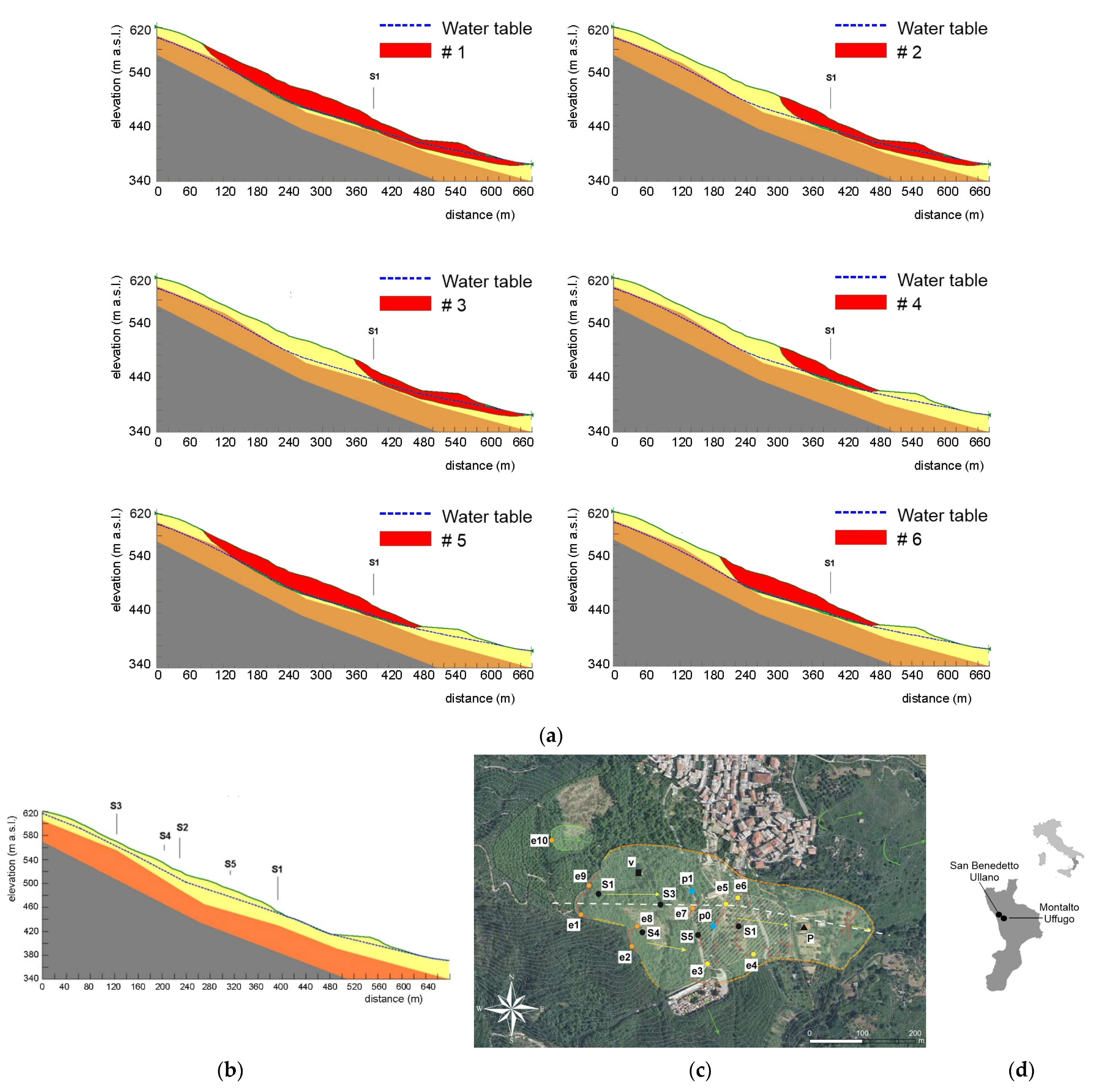
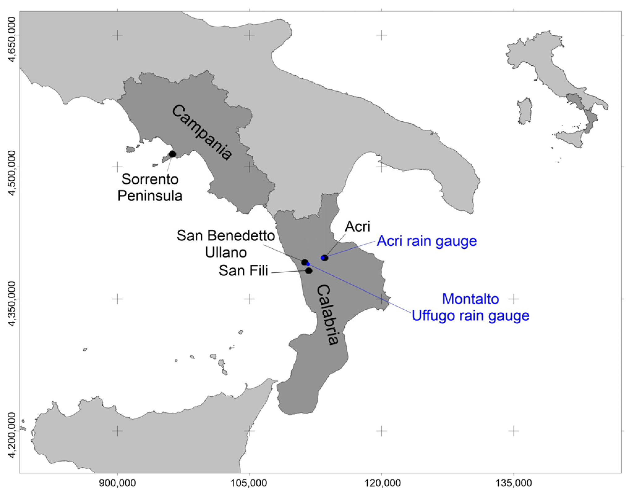
Iovine et al. [146] analysed the mobilisation of the San Rocco landslide at San Benedetto Ullano (Northern Calabria). A first phase of activation occurred from January to May 2009, and was followed by a reactivation on February 2010, after extraordinary rainfalls. During the 2–3 months antecedent to the 2009 mobilization, cumulated rains nearly matched the first two critical events even recorded at Montalto Uffugo—i.e., the closest rain gauge, 3.5 km away from the study case (cf. Figure 1)—since 1921 [21]. Based on monitored data, a parametric limit equilibrium back-analysis (LEM) was carried out to examine the stability conditions of the slope and to quantify the role of the fluctuations of groundwater levels.
As also testified by air-photo interpretation of 1954 and 1990 flight coverages (scale 1:35,000) by the IGM-Italian Military Geographic Institute, the landslide mobilisations could be interpreted as progressive reactivations of a large, dormant rock slide along pre-existing sliding surfaces (perhaps, with the only exception of its deepest portion). Recent phases of mobilisation apparently showed a marked enlarging trend, progressively involving wider and deeper sectors.
The geological scheme of the slope was refined by employing data collected through a set of explorative boreholes, equipped with inclinometers and piezometers, laboratory tests and the literature. The depth of the mobilised body varied between 15 m and 35 m. The scheme adopted for calculations consisted of an intact bedrock substrate, in turn overlain by weathered rocks (layer 2), and by a surficial gneissic detrital cover (layer 1). Accordingly, in the LEM analysis, the shear strength values were those at residual for layer 1 (γ = 17 kN/m3, c′ = 0 kPa, φ′ = 32°), in which most of the failure surface developed; as for its portion inside layer 2, it was assumed to be activated for the first time, and a friction angle slightly smaller than the peak value was assumed (γ = 18 kN/m3, c′ = 0 kPa, φ′ = 36°).
In the LEM analysis, six different sliding bodies were hypothesised (Figure 1a). A finite-element seepage analysis was preliminarily carried out to define the water regime in the slope associated with steady-state (summer) flow conditions. Results indicated a geometry of the water table in good agreement with field measurements, with water table at S1 (a borehole equipped with an open-pipe piezometer) about 19 m below the ground surface. As a consequence of infiltration, the water table could raise up closer to the surface during winter. As available data on the water table during considered activations was limited (levels were not measured during paroxysmal stages), the amounts considered in the parametric analyses were raised parallel to the summer configuration. In Figure 1b, the worst (winter) water table conditions, as assumed in the parametric analyses, are shown (with the water table at S1 about 4 m below the ground surface).
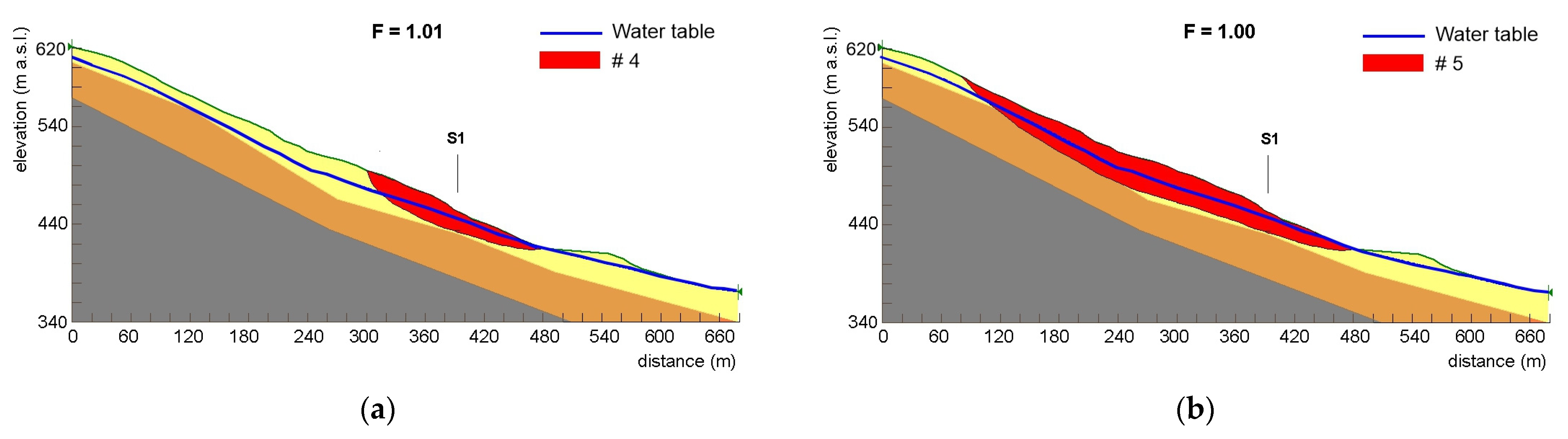
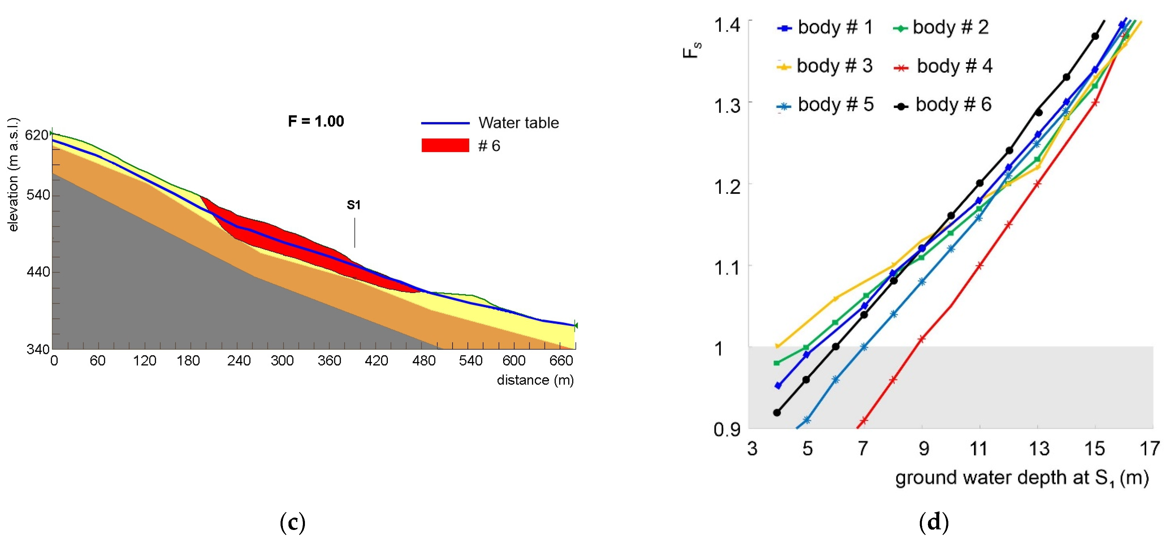
Starting from the summer regime, a sensitivity LEM study was performed by considering different geometries of the water table (Figure 2). The results of the sensitivity analysis, in terms of the safety factor of the six landslide bodies for different groundwater levels, suggested stable conditions (Fs > 1.5) in the case of the summer pore-water pressure regime. Body 4 becomes unstable when the water table at S1 is 9 m below the ground, approximating the surface downslope; in the case of the further raising of the water table, retrogressive activations involve bodies 5 and 6 with the water table at S1 7 m and 6 m, respectively.; bodies one and two become unstable only for shallower depths, followed by body three. If the water table reaches a depth of 4 m at S1, all the considered bodies are unstable.
The above modelling results are in quite good agreement with evidence observed in the field between January 2009 and February 2010 and are synthetised also in terms of the safety factor vs. water table depths in Figure 2d. In the absence of adequate slope remedial works, further landslide activations should therefore be expected according to the pattern described above, due to the rising of the groundwater table, with an initial activation of body four, and retrogressive evolution of the instability until it involves the portion of slope represented by body five.
In the emergency context of the San Rocco landslide activations, the choice of the LEM approach (instead of more sophisticated modelling alternatives) mainly depended on the need to obtain reliable results within a timeframe compatible with risk mitigation actions. Such an approach could be adopted thanks to the availability of suitable information on the geometry of the landslide body and on hydrogeological and geotechnical properties, as obtained through field and laboratory investigations. Finally, considering the shape of the slope movement, the adopted 2D scheme reasonably provided more conservative results, in terms of safety factor, with respect to 3D ones.
5.2. Application of Hydrological Modelling
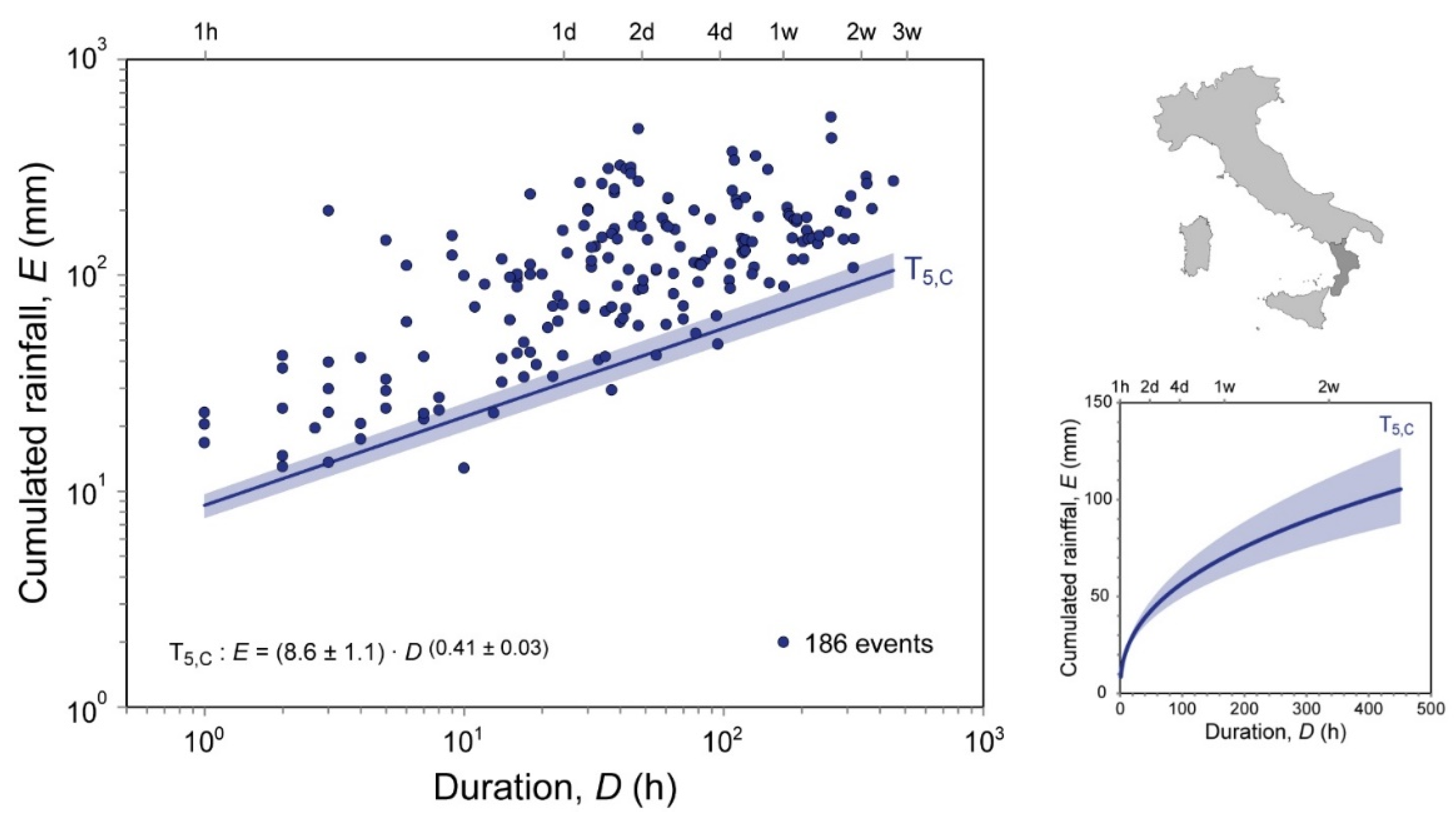
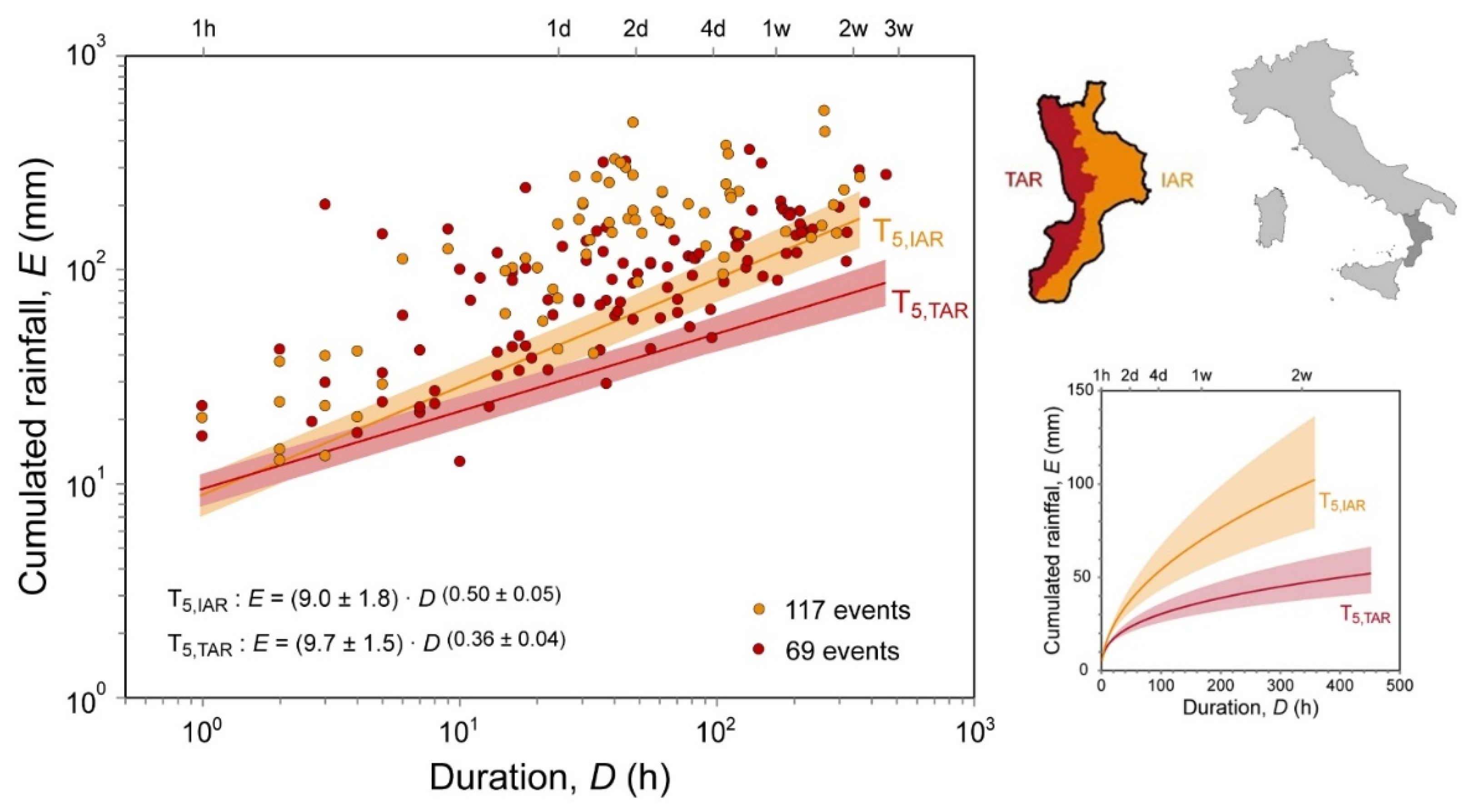
Vennari et al. [147] detected 186 rainfall events that triggered 251 shallow landslides in Calabria, from January 1996 to September 2011. The durations (D) of triggering rainfall events ranged from 1 to 451 h, with cumulated rainfall (E) from 12.8 to 542 mm. Authors identified a regional E-D threshold at the 5% exceedance probability level (T5,C), with associated uncertainties (Figure 3):
Furthermore, the role of the following environmental factors in the regional E-D threshold was investigated: lithological domains, soil regions, pluviometrical homogeneous regions (based on daily annual maxima), seasonal periods (wet/dry) and alert regions (Tyrrhenian/Ionian) as defined by the Italian Civil Protection Department. Unfortunately, due to the “limited” number of empirical data points, no further E-D thresholds could be obtained at the sub-regional level, except for the Tyrrhenian (T5,TAR) and Ionian (T5,IAR) alert regions (Figure 4):
For D > 24 h, the above thresholds are statistically different: lower E values are in fact expected in the Tyrrhenian alert region to trigger landslides with respect to the Ionian one.
In Sicily, Gariano et al. [16] identified 200 rain events that triggered 223 or more landslides between 2002 and 2011. The durations of rainfall events ranged from 1 to 254 h, with an average of 54.9 h, and E from 11.3 to 466.4 mm, with an average of 79.8 mm. Sicilian regional rainfall thresholds were defined for different exceedance probabilities (from 1% to 50%). A general methodology for the objective identification of thresholds, providing an optimal balance between the maximisation of correct predictions and minimisation of incorrect predictions, was proposed by the authors, including missed and false alarms. In such a study, the selection of the optimal threshold is based on three weighted skill scores (HK, POFA, and δ—this latter being the Euclidean distance from the ROC “perfect classification”), with the weights decided depending on the scope of the threshold. As a result, the 7% threshold performed the better compromise:
To allow for comparisons with other study regions, the 5% Sicilian threshold is:
Gariano et al. [16] also tried to investigate the influence of lithology and seasonality. Nevertheless, the limited size of the sample did not allow us to obtain reliable thresholds, except for those related to the East (EAR) and West (WAR) alert regions (Figure 5):
As a result, the T5,EAR threshold is steeper than T5,WAR. For D ≤ 12 h, a larger amount of cumulated rainfall is needed to trigger landslides in the WAR, whereas the opposite occurs for D > 12 h.
Overall, the above results can be used within early warning platforms, in support of the Civil Protection Department, such as in the case of the SANF, implemented by the CNR-IRPI [31]. The mentioned studies are characterised by a strong effort to objectivise the entire procedure, from the identification of triggering rain events to the definition of triggering thresholds for shallow landslides. However, problems related to the quantity and quality of information made the identification of the thresholds at the regional and sub-regional scales quite complex. The obtained E-D values, especially for the shortest time aggregations, appear rather modest, and could be affected by local conditions of greater “fragility” of the territory (e.g., due to artificial cuts).
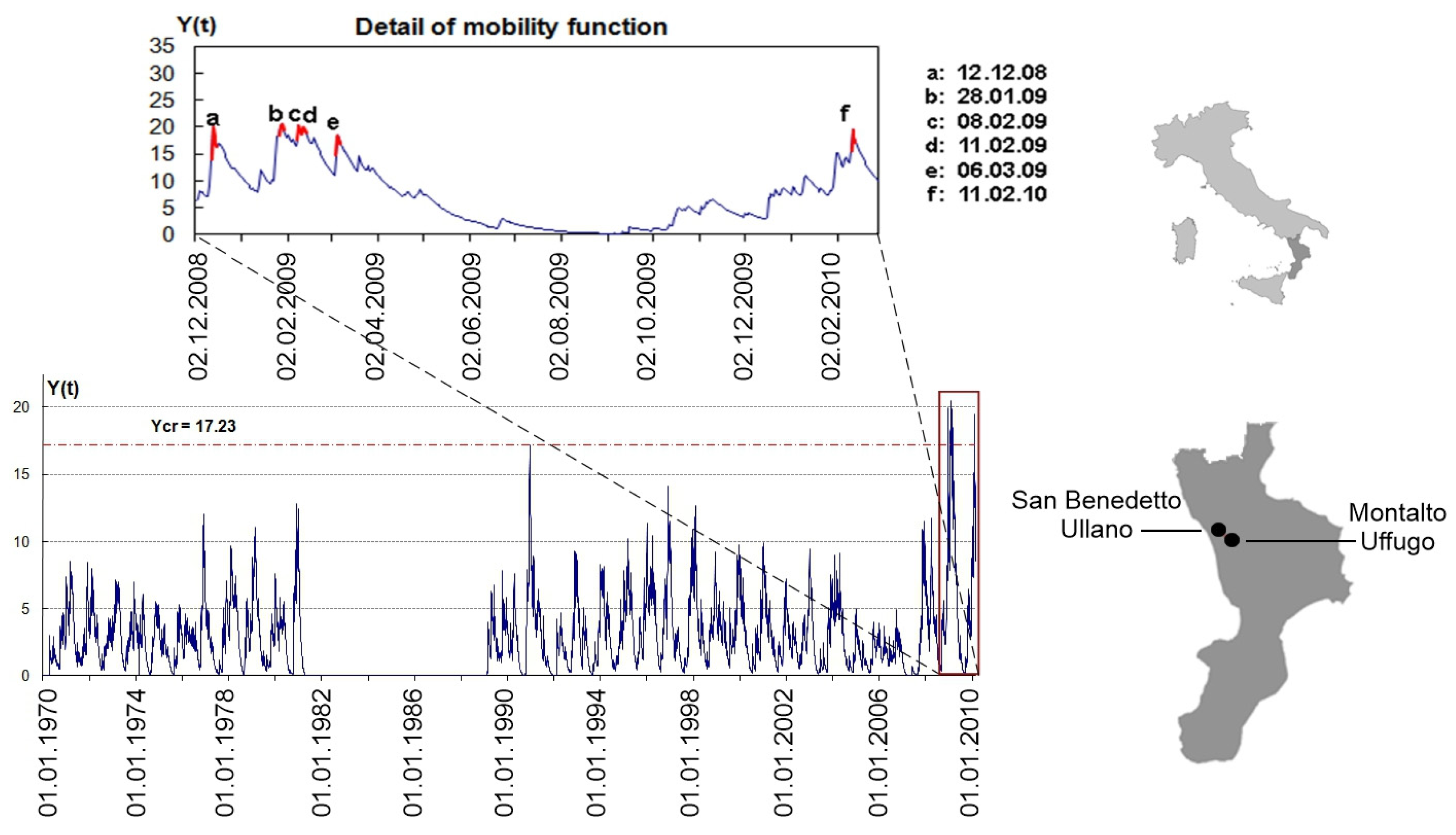
Capparelli et al. [117] applied the FLaIR model to the San Rocco landslide (cf. Section 5.1). Daily rainfall series recorded since 1970 at Montalto Uffugo and landslide activations (occurring on 28 January 2009 and 11 February 2010) were considered, along with the acceleration of surficial displacements detected on 8 and 11 February and on 6 March 2009. The filter function that best reproduced the above mobilisations was the gamma distribution with parameters: and days. The mobility function was identified by adopting a ranking criterion. The observed dates of mobilisation corresponded well with the predicted peaks (Figure 6).
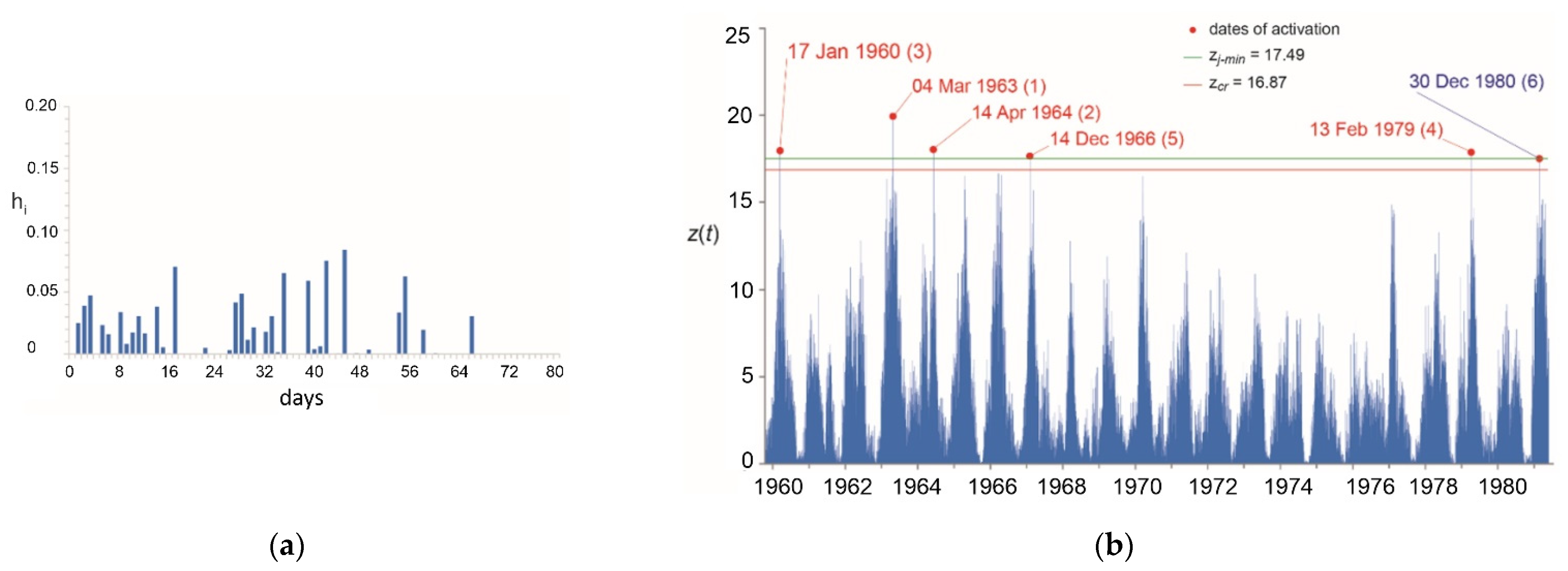
Terranova et al. [17] applied the GASAKe model to different case studies in Southern Italy, in particular, to three rockslides in Calabria (at Acri-Serra di Buda, San Benedetto Ullano-San Rocco and San Fili-Uncino) and to 11 events of widespread soil-slip activations in the Sorrento Peninsula, in Campania (Figure 7). For each case study, the model was first optimised by considering a subset of calibration dates and then validated against the remaining dates of activation (cf. Table 1).
According to Terranova et al. [17]:
- For the Campanian shallow landslides of the Sorrento Peninsula, the obtained is quite short (28 days), about a half of those obtained for the Calabrian rock slides (ranging between 46 and 74 days), thus confirming the expected direct relationship between base time, on one side, and the extent of instability masses and groundwater paths on the other -cf. [9].
- The best performances were observed for the San Fili-Uncino (Figure 8) and for the San Benedetto Ullano-San Rocco case studies, with neither missing nor false alarms both in calibration and in validation (in fact, even for this latter case, the predicted activation anticipates “only few hours”, the alarm issued by the public authority of Civil Protection, hence Φv is actually 100%).
- Less satisfactory results were instead obtained for the Sorrento Peninsula study case. In general, concerning shallow landslides, worse modelling results are intrinsically expected due to a number of reasons: the differences in extent of the triggered landslides, heterogeneities in slope materials, inhomogeneous rainfall fields (especially in case of short-lasting, high-intensity storms) and poor quality of rain data due to low density of the rain-gauge network. Moreover, some dates of activation may even be missing, especially in remote areas. Anyhow, despite all such limitations, Φ greater than 80% and 73% were obtained for calibration and validation in the Sorrento Peninsula, respectively.
- For the Acri case study, the application of the model was evidently hampered by misleading geotechnical information (cf. e.g., [148]), reflecting in the unsatisfactory values of Φ obtained both in calibration (ca. 83%) and especially in validation (ca. 62%). For this case study, some of the available dates of activation apparently refer to secondary portions of the main rockslide; historical archives did not permit an accurate understanding of the mobilised volumes, and then secondary movements (or even activations of different nearby phenomena) may have been incorrectly attributed to the investigated slope movement.
As based on a statistical approach, the above examples of hydrological modelling require appropriate calibration and validation phases and are highly dependent on the availability of data concerning past, known landslide activations (usually available only for urbanised areas) and on representative rainfall series. Despite the inherent limitations of any empirical approach, such models make it possible to quickly analyse information on individual case studies, or even on numerous phenomena of the same type within geologically homogeneous areas. Thanks to their less-demanding requirements, in terms of computing power and detailed geological information, with respect to physical methods, these (low-cost) models may profitably be employed to improve present-day early warning systems at either the local or sub-regional scales.
6. Conclusions and Some Research Perspectives
In this paper, a synthetic review of physical and hydrological models for predicting the critical conditions for the initiation of slope movements was discussed. In addition to models and procedures well-known in the literature, some recent models developed for research purposes were also presented. For both types of approaches, examples of applications to case studies in Southern Italy were shown, with comments on obtained performances.
As regards the physically based study carried out at San Benedetto Ullano, it could be realised thanks to a strict cooperation between the CNR-IRPI of Cosenza and the Major (local Authority of Civil Protection), aimed at supporting risk mitigation. The evolution of the landslide mobilisation was monitored by means of a remote network of superficial sensors (extensometers, clinometers and one rain gauge), combined with daily patrols by a team of volunteers properly trained for the purpose. In territorial contexts severely affected by slope instabilities, such as in Calabria, similar experiences are prototypical examples of support actions for municipalities that should rather be systematically provided by regional technical services.
The hydrological E-D studies in Calabria and in Sicily were realised in the frame of a national project, funded by the Civil Protection Department and aimed at implementing an early warning platform for shallow-landslide prediction in Italy. The main positives of this project rely on the standardisation efforts of the adopted procedure for threshold identification and on its easiness of use. In perspective, the antecedent conditions for soil moisture should be taken into account, as well as meteorological characteristics of the triggering events, in addition to lithological and morphological site characteristics.
The main merit of FLaIR lies in having extended a classic method, commonly applied to model the relationship between rainfall and runoff, to the relationship between rainfall and landslide activation. Further developments in such a type of approach led to the GA-based model SAKe, in which the shape of the Kernel is not described by prefixed mathematical functions. In such a way, the flexibility of the model made it possible to achieve far higher fitness values than with other models, especially in study cases characterised by several dates of activation. Its latest version (presently, undergoing test) strongly reduced the computing time and allows us to speculate on groundwater conditions, thanks to a regressive tool that synthetises the discretised the Kernel into a combination of analytical functions.
Generally speaking, modelling approaches, be it either physical or hydrological, are extremely useful tools for implementing early warning systems for landslides. Physical models generally suffer from limitations related to data availability and costs that restrict their applicability. Anyhow, susceptibility analyses performed with these models may be improved by considering the transient effects of rainfall on slopes. Hydrological models do not require detailed information on slope characteristics and are simpler to apply but are not physically based. To improve predictive performance and reliability, hydrological and physical approaches may be combined and integrated within decision support systems for risk mitigation purposes.
Both types of modelling approaches require updated, high-quality data extended over the whole area of interest. To this purpose, it would be desirable that services by regional authorities be strengthened to guarantee adequate surveying and monitoring activities, and to implement suitable geological/hydrological archives on relevant parameters (e.g., rainfall, temperature) and on slope movements (e.g., location, type, material characteristics, dates of activation). Concerning the rains, networks may be improved by implementing further gauges and meteor-radar installations. Moreover, piezometric levels could be continuously monitored at places of interest. Landslide displacements could be verified by means of several techniques (remote images, Synthetic Aperture Radar, Global Navigation Satellite Systems, photogrammetric cameras and Lidar) able to detect small displacement changes and deformation patterns, even in remote areas. On the other hand, to better investigate the phenomena underlying instability conditions (e.g., infiltration and distribution of pore pressures in saturated and unsaturated layers), well-equipped laboratory channels should be employed.
Still, in terms of perspectives, in the hydrological approach, efforts may be focused to extend its field of application to a regional scale (e.g., to “families” of similar phenomena potentially affecting a geological-homogeneous zone). In general, a reduction of the processing time could be achieved by means of software parallelisation, allowing for a more effective use within decision support systems for landslide-risk mitigation.
Author Contributions
Conceptualization, A.D., V.L., V.R., O.G.T. and G.I.; methodology, A.D., V.L., V.R., O.G.T. and G.I.; software, A.D., V.L., V.R., O.G.T. and G.I.; validation, A.D., V.L., V.R., O.G.T. and G.I.; formal analysis, A.D., V.L., V.R., O.G.T. and G.I.; investigation, A.D., V.L., V.R., O.G.T. and G.I.; resources, A.D., V.L., V.R., O.G.T. and G.I.; data curation, A.D., V.L., V.R., O.G.T. and G.I.; writing—original draft preparation, A.D., V.L., V.R., O.G.T. and G.I.; writing—review and editing, A.D., V.L., V.R., O.G.T. and G.I.; visualization, A.D., V.L., V.R., O.G.T. and G.I.; supervision, A.D., V.L., V.R., O.G.T. and G.I.; project administration, A.D., V.L., V.R., O.G.T. and G.I.; funding acquisition, A.D., V.L., V.R., O.G.T. and G.I. All authors have read and agreed to the published version of the manuscript.
Funding
This research received no external funding.
Data Availability Statement
Not applicable.
Conflicts of Interest
The authors declare no conflict of interest.
Appendix A
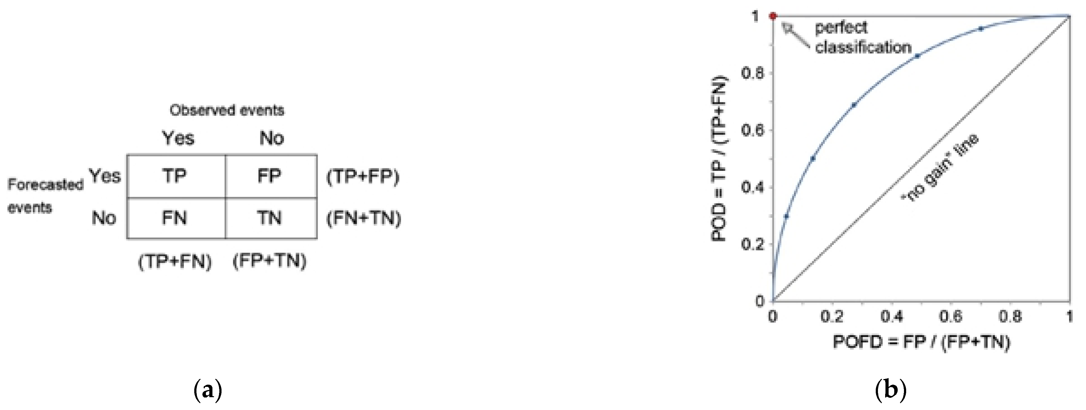
With reference to Figure A1, event occurrences can be true (T) or false (F), whereas predictions can be successful (P) or wrong (N). Furthermore, a true positive (TP) corresponds to a modelled rain condition above the threshold that resulted in (at least) one landslide activation, whereas a true negative (TN) lies below the threshold and did not result in any landslide activation. On the contrary, a false positive (FP) corresponds to a modelled rainfall condition above the threshold that did not result in any landslide activation; a false negative (FN) lies below the threshold, but landslide occurrences are recorded.
Figure A1.
(a) Contingency table showing the four possible outcomes of a binary classifier model. TP = True Positive, TN = True Negative, FP = False Positive, FN = False Negative. (b) Receiver Operating Characteristic (ROC) space, with hypothetical model results. POD = Probability of Detection, POFD = Probability of False Detection (modified after [16]).

For a landslide warning system, FP are “false alarms” and FN are “missed alarms”. When using high thresholds, the number of FN increases, and that of TP decreases correspondingly. Conversely, when using low thresholds, the number of FP increases and that of TN decreases.
The above concepts, and proper skill scores, e.g., Probability of Detection (POD), Probability of False Detection (POFD), Probability of False Alarms (POFA), Hanssen and Kuipers (HK) (cf. [16] and Table A1, for more details), must be considered for evaluating the performance of any modelling approach. In particular, in the ROC (Receiver Operating Characteristic [149,150])-space, each point represents the prediction capability of a given threshold. The ROC curve is obtained by varying the exceedance probability, thus obtaining different thresholds. The best prediction performance (i.e., characterised by neither FN nor FP) corresponds to the upper left corner of the ROC plot (perfect classification). The closer the point to the perfect classification, the better the model prediction skill: this is achieved when POD increases and POFD decreases. Points located in the lower left side of the ROC plot correspond to a prediction with few TPs and FPs. Conversely, points in the upper right side correspond to a prediction with many TPs and FPs. Note that a random guess would give a point along the no-gain line, i.e., the diagonal from the left bottom to the top right corners of the ROC plot.

Table A1.
Skill scores based on contingencies shown in Figure A1 used to perform the validation of the thresholds. TP = true positives, FP = false positives, FN = false negatives, TN = true negatives (according to [16]).
| Skill Score | Formula | Range | Optimal Value |
|---|---|---|---|
| Probability of Detection | [0, 1] | 1 | |
| Probability of False Detection | [0, 1] | 0 | |
| Probability of False Alarms | [0, 1] | 1 | |
| Hanssen and Kuipers | [−1, 1] | 1 |
References
- Popescu, M.E. Landslide causal factors and landslide remedial options. In Proceedings of the 3rd International Conference on Landslides, Slope Stability and Safety of Infrastructures, Singapore, 11–12 July 2002. [Google Scholar]
- Peranić, J.; Čeh, N.; Arbanas, Ž. The use of soil moisture and pore-water pressure sensors for the interpretation of landslide behaviour in small-scale physical models. Sensors 2022, 22, 7337. [Google Scholar] [CrossRef] [PubMed]
- Campbell, R.H. Debris flow originating from soil slip during rainstorm in southern California. Q. J. Eng. Geol. Hydrogeol. 1975, 7, 377–384. [Google Scholar] [CrossRef]
- De Vita, P.; Piscopo, V. Influences of hydrological and hydrogeological conditions on debris flows in peri-vesuvian hillslopes. Nat. Hazards Earth Syst. Sci. 2002, 2, 27–35. [Google Scholar] [CrossRef]
- Fiorillo, F.; Esposito, L.; Grelle, G.; Revellino, P.; Guadagno, F.M. Further hydrological analyses on landslide initiation in the Sarno area (Italy). Ital. J. Geosci. 2013, 132, 341–349. [Google Scholar] [CrossRef]
- Schilirò, L.; Poueme Djueyep, G.; Esposito, C.; Scarascia Mugnozza, G. The role of initial soil conditions in shallow landslide triggering: Insights from physically based approaches. Geofluids 2019, 2019, 2453786. [Google Scholar] [CrossRef] [Green Version]
- Fredlund, D.G.; Rahardjo, H. Soil Mechanics for Unsaturated Soils; John Wiley & Sons, Inc.: New York, NY, USA, 1993; 544p. [Google Scholar]
- Brand, E.W. Landslides in Southeast Asia: A state-of-the-art report. In Proceedings of the IV International Symposium on Landslides, Canadian Geotechnical Society, Toronto, ON, Canada, 16–21 September 1984. [Google Scholar]
- Cascini, L.; Versace, P. Eventi pluviometrici e movimenti franosi. In Proceedings of the XVI Convegno Nazionale di Geotecnica, Bologna, Italy, 14–16 May 1986. (In Italian). [Google Scholar]
- Cascini, L.; Versace, P. Relationship between rainfall and landslide in a gneissic cover. In Proceedings of the Fifth International Symposium on Landslides, Lausanne, Switzerland, 10–15 July 1988. [Google Scholar]
- Wieczorek, G.F. Landslide Triggering Mechanisms. In Landslides: Investigation and Mitigation; Turner, A.K., Schuster, R.L., Eds.; National Academy Press: Washington, DC, USA, 1996; pp. 76–90. [Google Scholar]
- Van Asch, T.W.J.; Buma, J.; Van Beek, L.P.H. A view on some hydrological triggering systems in landslides. Geomorphology 1999, 30, 25–32. [Google Scholar] [CrossRef]
- Jakob, M.; Weatherly, H. A hydroclimatic threshold for landslide initiation on the North Shore Mountains of Vancouver, British Columbia. Geomorphology 2003, 54, 137–156. [Google Scholar] [CrossRef]
- Guzzetti, F.; Gariano, S.L.; Peruccacci, S.; Brunetti, M.T.; Melillo, M. Rainfall and landslide initiation. In Rainfall—Modeling, Measurement and Applications, 1st ed.; Morbidelli, R., Ed.; Elsevier: Amsterdam, The Netherlands, 2022; pp. 427–450. [Google Scholar]
- Aleotti, P. A warning system for rainfall-induced shallow failures. Eng. Geol. 2004, 73, 247–265. [Google Scholar] [CrossRef]
- Gariano, S.L.; Brunetti, M.T.; Iovine, G.; Melillo, M.; Peruccacci, S.; Terranova, O.; Vennari, C.; Guzzetti, F. Calibration and validation of rainfall thresholds for shallow landslide forecasting in Sicily, southern Italy. Geomorphology 2015, 228, 653–665. [Google Scholar] [CrossRef]
- Terranova, O.; Gariano, S.L.; Iaquinta, P.; Lupiano, V.; Rago, V.; Iovine, G. Example of application of GASAKe for predicting the occurrence of rainfall-induced landslides in Southern Italy. Geoscience 2018, 8, 78. [Google Scholar] [CrossRef]
- Zaruba, Q. Vliv klimatických poměrů na smršťování křídových slínů. Věda přír 1936, 17, 217–231. [Google Scholar]
- Capparelli, G.; Versace, P. FLaIR and SUSHI: Two mathematical models for early warning of landslides induced by rainfall. Landslides 2011, 8, 67–79. [Google Scholar] [CrossRef]
- Cauvin, S.; Cordier, M.O.; Dousson, C.; Laborie, P.; Lévy, F.; Montmain, J.; Porcheron, M.; Servet, I.; Travé-Massuyès, L. Monitoring and alarm interpretation in industrial environments. AI Commun. 1998, 11, 139–173. [Google Scholar]
- Iovine, G.; Iaquinta, P.; Terranova, O. Emergency management of landslide risk during autumn-winter 2008/2009 in Calabria (Italy), The example of San Benedetto Ullano. Proceedings of 18th World IMACS Congress and MODSIM09 International Congress on Modelling and Simulation, Cairns, Australia, 13–17 July 2009. [Google Scholar]
- Carter, J. The Notion of Threshold: An Investigation into Conceptual Accompaniment in Aristotle and Hegel, Conserveries Mémorielles 2010, 7. Available online: http://cm.revues.org/431 (accessed on 17 October 2022).
- White, I.D.; Mottershead, D.N.; Harrison, J.J. Environmental Systems, 2nd ed.; Chapman & Hall: London, UK, 1996; 616p. [Google Scholar]
- Wilks, D.S. Statistical Methods in the Atmospheric Sciences; Academic Press: San Diego, CA, USA, 1995; 467p. [Google Scholar]
- Accadia, C.; Mariani, S.; Casaioli, M.; Lavagnini, A.; Speranza, A. Sensitivity of precipitation forecast skill scores to bilinear interpolation and a simple nearest-neighbor average method on high-resolution verification grids. Weather. Forecast. 2003, 18, 918–932. [Google Scholar] [CrossRef]
- Staley, D.M.; Kean, J.W.; Cannon, S.H.; Schmidt, K.M.; Laber, J.L. Objective definition of rainfall intensity–duration thresholds for the initiation of post-fire debris flows in southern California. Landslides 2013, 10, 547–562. [Google Scholar] [CrossRef]
- Mirus, B.B.; Morphew, M.D.; Smith, J.B. Developing hydro-meteorological thresholds for shallow landslide initiation and early warning. Water 2018, 10, 1274. [Google Scholar] [CrossRef] [Green Version]
- Keefer, D.K.; Wilson, R.C.; Mark, R.K.; Brabb, E.E.; Brown, W.M., III; Ellen, S.D.; Harp, E.L.; Wieczorek, G.F.; Alger, C.S.; Zatkin, R.S. Real-time Landslide Warning During Heavy Rainfall. Science 1987, 238, 921–925. [Google Scholar] [CrossRef]
- Baum, R.L.; Godt, J.W. Early warning of rainfall-induced shallow landslides and debris flows in the USA. Landslides 2010, 7, 259–272. [Google Scholar] [CrossRef]
- Piciullo, L.; Gariano, S.L.; Melillo, M.; Brunetti, M.T.; Peruccacci, S.; Guzetti, F.; Calvello, M. Definition and performance of a threshold-based regional early warning model for rainfall-induced landslides. Landslides 2017, 14, 995–1008. [Google Scholar] [CrossRef]
- Rossi, M.; Peruccacci, S.; Brunetti, M.T.; Marchesini, I.; Luciani, S.; Ardizzone, F.; Balducci, V.; Bianchi, C.; Cardinali, M.; Fiorucci, F.; et al. SANF: National warning system for rainfall-induced landslides in Italy. Proceedings of 11th International and 2nd North American Symposium on Landslides and Engineered Slopes, Banff, AB, Canada, 3–8 June 2012. [Google Scholar]
- Chung, C.J.F.; Fabbri, A.G. Validation of spatial prediction models for landslide hazard mapping. Nat. Hazards 2003, 30, 451–472. [Google Scholar] [CrossRef]
- Lee, G.; Kim, W.; Oh, H.; Youn, B.D.; Kim, N.H. Review of statistical model calibration and validation—From the perspective of uncertainty structures. Struct. Multidiscip. Optim. 2019, 60, 1619–1644. [Google Scholar] [CrossRef]
- Saltelli, A. Sensitivity Analysis for Importance Assessment. Risk Anal. 2002, 22, 579–590. [Google Scholar] [CrossRef] [PubMed]
- Terzaghi, K. Stability of steep slopes on hard unweathered rock. Geotechnique 1962, 12, 251–270. [Google Scholar] [CrossRef]
- Johnson, A.M. Debris flow. In Slope Instability; Brunsden, D., Prior, D.B., Eds.; Wiley: Chichester, UK, 1984; pp. 257–361. [Google Scholar]
- Montgomery, D.R.; Dietrich, W.E. A physically-based model for the topographic control on shallow landsliding. Water Resour. Res. 1994, 30, 1153–1171. [Google Scholar] [CrossRef]
- Wilson, R.C.; Wieczorek, G.F. Rainfall thresholds for the initiation of debris flow at La Honda, California. Environ. Eng. Geosci. 1995, 1, 11–27. [Google Scholar] [CrossRef]
- Crosta, G.B. Regionalization of rainfall thresholds: An aid to landslide hazard evaluation. Environ. Geol. 1998, 35, 131–145. [Google Scholar] [CrossRef]
- Terlien, M.T.J. The determination of statistical and deterministic hydrological landslide-triggering thresholds. Environ. Geol. 1998, 35, 125–130. [Google Scholar] [CrossRef]
- Crosta, G.B.; Dal Negro, P.; Frattini, P. Soil slips and debris flows on terraced slopes. Nat. Hazards Earth Syst. Sci. 2003, 3, 31–42. [Google Scholar] [CrossRef] [Green Version]
- Pisani, G.; Castelli, M.; Scavia, C. Hydrogeological model and hydraulic behaviour of a large landslide in the Italian Western Alps. Nat. Hazards Earth Syst. Sci. 2010, 10, 2391–2406. [Google Scholar] [CrossRef] [Green Version]
- Van Asch, T.W.J.; Sukmantalya, I.N. The modelling of soil slip erosion in the upper Komering area, South Sumatra Province, Indonesia. Geogr. Fis. Din. Quat. 1993, 16, 81–86. [Google Scholar]
- Terlien, M.J.M. Modelling Spatial and Temporal Variations in Rainfall-Triggered Landslides; International Institute for Aerospace Survey and Earth Sciences (ITC): Enschede, The Netherlands, 1996; 254p. [Google Scholar]
- Chen, H.; Dadson, S.; Chi, Y. Recent rainfall-induced landslides and debris flow in northern Taiwan. Geomorphology 2006, 77, 112–125. [Google Scholar] [CrossRef]
- Jamaludin, S.; Ali, F. An overview of some empirical correlations between rainfall and shallow landslides and their applications in Malaysia. Electron. J. Geotech. Eng. 2011, 16, 1429–1440. [Google Scholar]
- Huang, Y.H. Slope Stability Analysis by the Limit Equilibrium Method: Fundamentals and Methods; ASCE Press: Reston, VA, USA, 2014; p. 363. [Google Scholar]
- Janbu, N. Application of composite slip surfaces for stability analysis. In Proceedings of the European Conference on Stability of Earth Slopes, Stockholm, Sweden, 20–25 September 1954. [Google Scholar]
- Bishop, A.W. The use of the slip circle in the stability analysis of slopes. Géotechnique 1955, 5, 7–17. [Google Scholar] [CrossRef]
- Morgenstern, N.R.; Price, V.E. The analysis of the stability of general slip surfaces. Géotechnique 1965, 15, 79–93. [Google Scholar] [CrossRef]
- Spencer, E. A method of analysis of the stability of embankments assuming parallel inter-slice forces. Géotechnique 1967, 17, 11–26. [Google Scholar] [CrossRef]
- Sarma, S.K. Stability analysis of embankments and slopes. Géotechnique 1973, 23, 423–433. [Google Scholar] [CrossRef]
- Anagnosti, P. Three-dimensional stability of fill dams. In Proceedings of the 7th International Conference on soil Mechanics and Foundation Engineering, Mexico City, Mexico, 29 August 1969; Volume 2, pp. 275–280. [Google Scholar]
- Kumar, S.; Choudhary, S.S.; Burman, A. Recent advances in 3D slope stability analysis: A detailed review. Model. Earth Syst. Environ. 2022, 1–18. [Google Scholar] [CrossRef]
- Quecedo, M.; Pastor, M.; Herreros, M.I. Numerical modelling of impulse wave generated by fast landslides. Int. J. Numer. Methods Eng. 2004, 59, 1633–1656. [Google Scholar] [CrossRef]
- Baligh, M.M.; Azzouz, A.S. End Effects of Stability of Cohesive Slopes. J. Geotech. Eng. Div. 1975, 101, 1105–1117. [Google Scholar] [CrossRef]
- Chen, R.H. Three-Dimensional Slope Stability Analysis; Report JHRP-81-17; Purdue University: West Lafayette, IN, USA, 1981. [Google Scholar]
- Gens, A.; Hutchinson, J.N.; Cavounidis, S. Three-Dimensional Analysis of Slides in Cohesive Soils. Geotechnique 1988, 38, 1–23. [Google Scholar] [CrossRef]
- Stark, T.D.; Eid, H.T. Performance of Three-Dimensional Slope Stability Methods in Practice. J. Geotech. Geoenviron. Eng. 1998, 124, 1049–1060. [Google Scholar] [CrossRef]
- Arellano, D.; Stark, T.D. Importance of Three-Dimensional Slope Stability Analises in practice. In Proceedings of the Sessions of Geo-Denver 2000, Denver, CO, USA, 5–8 August 2000; ASCE: Reston, VA, USA, 2000; pp. 18–32. [Google Scholar]
- Shen, J.; Karakus, M. Three-dimensional numerical analysis for rock slope stability using shear strength reduction method. Can. Geotech. J. 2014, 51, 164–172. [Google Scholar] [CrossRef]
- Reid, M.E.; Christian, S.B.; Brien, D.L.; Henderson, S. Scoops3D—Software to Analyze Three-Dimensional Slope Stability throughout a Digital Landscape; US Geological Survey: Reston, VA, USA, 2015. [Google Scholar]
- Borselli, L. “SSAP 5.1—“Slope Stability Analysis Program”. Manuale di Riferimento del Codice SSAP Versione 5.1. 2022. Available online: https://doi.org/10.13140/RG.2.2.31522.91841 (accessed on 5 September 2022).
- Innocenti, A.; Pazzi, V.; Borselli, L.; Nocentini, M.; Lombardi, L.; Gigli, G.; Fanti, R. Reconstruction of the evolution phases of a landslide by using multi-layer back-analysis methods. Landslides 2023, 20, 189–207. [Google Scholar] [CrossRef]
- Hoek, E.; Brown, E.T. The Hoek–Brown failure criterion and GSI—2018 edition. J. Rock Mech. Geotech. Eng. 2019, 11, 445–463. [Google Scholar] [CrossRef]
- Carranza-Torres, C. Elasto-plastic solution of tunnel problems using the generalized form of the Hoek-Brown failure criterion. Int. J. Rock Mech. Min. Sci. 2004, 41, 629–639. [Google Scholar] [CrossRef]
- Barton, N.; Bandis, S.C. Review of predictive capability of JRC-JCS model in engineering practice. In Proceedings of the International Symposium on Rock Joints, Loen, Norway, 4–6 June 1990. [Google Scholar]
- Barton, N. Shear strength criteria for rock, rock joints, rockfill and rock masses: Problems and some solutions. J. Rock Mech. Geotech. Eng. 2013, 5, 249–261. [Google Scholar] [CrossRef] [Green Version]
- Olson, S.M.; Stark, T.D. Yield strength ratio and liquefaction analysis of slopes and embankments. J. Geotech. Geoenviron. Eng. 2003, 129, 727–737. [Google Scholar] [CrossRef] [Green Version]
- Dietrich, W.E.; Wilson, C.J.; Montgomery, D.R.; McKean, J.; Bauer, R. Erosion thresholds and land surface morphology. Geology 1992, 20, 675–679. [Google Scholar] [CrossRef]
- Dietrich, W.E.; Wilson, C.J.; Montgomery, D.R.; McKean, J. Analysis of erosion thresholds, channel networks, and landscape morphology using a digital terrain model. J. Geol. 1993, 101, 259–278. [Google Scholar] [CrossRef] [Green Version]
- Borga, M.; Dalla Fontana, G.; Cazorzi, F. Analysis of topographic and climatic control on rainfall-triggered shallow landsliding using a quasi-dynamic wetness index. J. Hydrol. 2002, 268, 56–71. [Google Scholar] [CrossRef]
- Lanni, C.; Borga, M.; Rigon, R.; Tarolli, P. Modelling shallow landslide susceptibility by means of a subsurface flow path connectivity index and estimates of soil depth spatial distribution. Hydrol. Earth Syst. Sci. 2012, 16, 3959–3971. [Google Scholar] [CrossRef] [Green Version]
- Baum, R.L.; Savage, W.Z.; Godt, J.W. TRIGRS—A Fortran Program for Transient Rainfall Infiltration and Grid-Based Regional Slope-Stability Analysis, Version 2.0; U.S. Geological Survey: Reston, VA, USA, 2009; 75p. [Google Scholar]
- Iverson, R.M. Landslide triggering by rain infiltration. Water Resour. Res. 2000, 36, 1897–1910. [Google Scholar] [CrossRef] [Green Version]
- Baum, R.L.; Godt, J.W.; Savage, W.Z. Estimating the timing and location of shallow rainfall-induced landslides using a model for transient, unsaturated infiltration. J. Geophys. Res. F Earth Surf. 2010, 115. [Google Scholar] [CrossRef]
- Liao, Z.; Hong, Y.; Kirschbaum, D.; Adler, R.F.; Gourley, J.J.; Wooten, R. Evaluation of TRIGRS (transient rainfall infiltration and grid-based regional slope-stability analysis)’s predictive skill for hurricane-triggered landslides: A case study in Macon County, North Carolina. Nat. Hazards 2011, 58, 325–339. [Google Scholar] [CrossRef]
- Park, D.W.; Nikhil, N.V.; Lee, S.R. Landslide and debris flow susceptibility zonation using TRIGRS for the 2011 Seoul landslide event. Nat. Hazards Earth Syst. Sci. 2013, 11, 2833–2849. [Google Scholar] [CrossRef] [Green Version]
- Grelle, G.; Soriano, M.; Revellino, P.; Guerriero, L.; Anderson, L.G.; Diambra, A.; Fiorillo, F.; Esposito, E.; Diodato, N.; Guadagno, F.M. Space–time prediction of rainfall-induced shallow landslides through a combined probabilistic/deterministic approach, optimized for initial water table conditions. Bull. Eng. Geol. Environ. 2014, 73, 877–890. [Google Scholar] [CrossRef]
- Salciarini, D.; Fanelli, G.; Tamagnini, C. A probabilistic model for rainfall—Induced shallow landslide prediction at the regional scale. Landslides 2017, 14, 1731–1746. [Google Scholar] [CrossRef]
- Ciurleo, M.; Mandaglio, M.C.; Moraci, N. A quantitative approach for debris flow inception and propagation analysis in the lead up to risk management. Landslides 2021, 18, 2073–2093. [Google Scholar] [CrossRef]
- Troncone, A.; Pugliese, L.; Conte, E. Rainfall threshold for shallow landslide triggering due to rising water table. Water 2022, 14, 2966. [Google Scholar] [CrossRef]
- Troncone, A.; Pugliese, L.; Conte, E. A simplified analytical method to predict shallow landslides induced by rainfall in unsaturated soils. Water 2022, 14, 3180. [Google Scholar] [CrossRef]
- Fenti, V.; Silvano, S.; Carampin, R. Quadro d’insieme sulla franosità e i dissesti nel bacino del T. Fiorentina (Belluno). Studi Trentini Sci. Nat. Acta Geol. 1984, 61, 3–31. [Google Scholar]
- Govi, M.; Mortara, G.; Sorzana, P.F. Eventi idrologici e frane. Geol. Appl. Idrogeol. 1985, 20, 359–375. [Google Scholar]
- Cannon, S.H.; Ellen, S.D. Rainfall conditions for abundant debris avalanches, San Francisco Bay region, California. Calif. Geol. 1985, 38, 267–272. [Google Scholar]
- Cancelli, A.; Nova, R. Landslides in Soil Debris Cover triggered by Rainstorms in Valtellina (Central Alps—Italy). In Proceedings of the IV International Conference and Field Workshop on Landslides, Tokyo, Japan, 23–31 August 1985; pp. 267–272. [Google Scholar]
- Sangrey, D.A.; Harrop-Williams, K.O.; Klaiber, J.A. Predicting ground-water response to precipitation. J. Geotech. Eng. 1984, 110, 957–975. [Google Scholar] [CrossRef]
- Crozier, M.J. Landslides: Causes, Consequences and Environment; Croom Helm: London, UK, 1986; 252p. [Google Scholar]
- Owen, R.C. Soil strength and microclimate in the distribution of shallow landslides. J. Hydrol. 1981, 20, 17–26. [Google Scholar]
- Guzzetti, F.; Peruccacci, S.; Rossi, M.; Stark, C.P. Rainfall thresholds for the initiation of landslides in central and southern Europe. Meteorol. Atmos. Phys. 2007, 98, 239–267. [Google Scholar] [CrossRef]
- Guzzetti, F.; Peruccacci, S.; Rossi, M.; Stark, C.P. The rainfall intensity-duration control of shallow landslides and debris flow: An update. Landslides 2008, 5, 3–17. [Google Scholar] [CrossRef]
- Dolojan, N.L.J.; Moriguchi, S.; Hashimoto, M.; Terada, K. Mapping method of rainfall-induced landslide hazards by infiltration and slope stability analysis. Landslides 2021, 18, 2039–2057. [Google Scholar] [CrossRef]
- Caine, N. The rainfall intensity-duration control of shallow landslides and debris flows. Geogr. Ann. Ser. A Phys. 1980, 62A, 23–27. [Google Scholar]
- Polloni, G.; Ceriani, M.; Lauzi, S.; Padovan, N.; Crosta, G. Rainfall and soil slipping events in Valtellina. In Proceedings of the Sixth International Symposium on Landslides, Christchurch, New Zealand, 10–14 February 1992. [Google Scholar]
- Brunetti, M.T.; Peruccacci, S.; Rossi, M.; Luciani, S.; Valigi, D.; Guzzetti, F. Rainfall thresholds for the possible occurrence of landslides in Italy. Nat. Hazards Earth Syst. Sci. 2010, 10, 447–458. [Google Scholar] [CrossRef]
- Lumb, P. Slope failures in Hong Kong. Q. J. Eng. Geol. 1975, 8, 31–65. [Google Scholar] [CrossRef]
- Chun, K.W.; Kim, M.; Catani, F.; Choi, B.; Seo, J.I. Effect of antecedent rainfall conditions and their variations on shallow landslide-triggering rainfall thresholds in South Korea. Landslides 2021, 18, 569–582. [Google Scholar]
- Kim, S.K.; Hong, W.P.; Kim, Y.M. Prediction of rainfall triggered landslides in Korea. In Proceedings of the VI International Symposium on Landslides, Christchurch, New Zealand, 10–14 February 1992. [Google Scholar]
- Page, M.J.; Trustrum, N.A.; De Rose, R.C. A high-resolution record of storm-induced erosion from lake sediments, New Zealand. J. Paleolimnol. 1994, 11, 333–348. [Google Scholar] [CrossRef]
- Brunsden, D. Mudslides. In Slope Instability; Brunsden, D., Prior, D.B., Eds.; John Wiley & Sons: London, UK, 1984; pp. 363–418. [Google Scholar]
- Polemio, M.; Sdao, F. The role of rainfall in the landslide hazard: The case of the Avigliano urban area (southern Apennines, Italy). Eng. Geol. 1999, 53, 297–309. [Google Scholar] [CrossRef]
- Bonnard, C.; Noverraz, F. Influence of climate change on large landslides: Assessment of long-term movements and trends. In Proceedings of the International Conference on Landslides: Causes Impact and Countermeasures, Davos, Switzerland, 17–21 June 2001. [Google Scholar]
- Zêzere, J.L.; Rodrigues, M.L. Rainfall thresholds for landsliding in Lisbon area (Portugal). In Landslides; Rybář, J., Stemberk, J., Wagner, P., Eds.; A.A. Balkema: Lisse, The Netherlands, 2002; pp. 333–338. [Google Scholar]
- Trigo, R.M.; Zêzere, J.L.; Rodrigues, M.L.; Trigo, I.F. The influence of the North Atlantic Oscillation on rainfall triggering of Landslides near Lisbon. Nat. Hazards 2005, 36, 331–354. [Google Scholar] [CrossRef]
- Wieczorek, G.F. Effect of rainfall intensity and duration on debris flows in central Santa Cruz Mountains, California, In Debris Flows/Avalanches: Processes, Recognition and Mitigation; Costa, J.E., Wieczorek, G.F., Eds.; Geological Society of America: Boulder, CO, USA, 1987; Volume VII, pp. 93–104. [Google Scholar]
- Flentje, P.; Chowdhury, R. Slope instability, hazard and risk associated with a rainstorm event: A case study. In Proceedings of the 8th International Symposium on Landslides, Cardiff, UK, 23–26 June 2000. [Google Scholar]
- Dikau, R.; Schrott, L. The temporal stability and activity of landslides in Europe with respect to climatic change (TESLEC): Main objectives and results. Geomorphology 1999, 30, 1–12. [Google Scholar] [CrossRef]
- Corominas, J. Landslides and climate. Keynote lecture. In Proceedings of the 8th International Symposium on Landslides, Cardiff, UK, 26–30 June 2000. [Google Scholar]
- Marques, R.; Zêzere, J.; Trigo, R.; Gaspar, J.; Trigo, I. Rainfall patterns and critical values associated with landslides in Povoação County (São Miguel Island, Azores): Relationships with the North Atlantic Oscillation. Hydrol. Process. 2008, 22, 478–494. [Google Scholar] [CrossRef]
- D’Ippolito, A.; Ferrari, E.; Iovino, F.; Nicolaci, A.; Veltri, A. Reforestation and land use change in a drainage basin of Southern Italy. iForest 2013, 6, 175–182. [Google Scholar] [CrossRef] [Green Version]
- D’Ippolito, A.; Calomino, F.; Alfonsi, G.; Lauria, A. Flow resistance in open channel due to vegetation at reach scale: A review. Water 2021, 13, 116. [Google Scholar] [CrossRef]
- D’Ippolito, A.; Calomino, F.; Alfonsi, G.; Lauria, A. Drag coefficient of in-line emergent vegetation in open channel flow. Int. J. River Basin Manag. 2021, 15, 329–334. [Google Scholar] [CrossRef]
- Penna, N.; Coscarella, F.; D’Ippolito, A.; Gaudio, R. Bed roughness effects on the turbulence characteristics of flows through emergent rigid vegetation. Water 2020, 12, 2401. [Google Scholar] [CrossRef]
- Penna, N.; Coscarella, F.; D’Ippolito, A.; Gaudio, R. Effects of fluvial instability on the bed morphology in vegetated channels. Environ. Fluid Mech. 2022, 22, 619–644. [Google Scholar] [CrossRef]
- D’Ippolito, A.; Calomino, F.; Penna, N.; Dey, S.; Gaudio, R. Simulation of accelerated subcritical flow profiles in an open channel with emergent rigid vegetation. Appl. Sci. 2022, 12, 6960. [Google Scholar] [CrossRef]
- Capparelli, G.; Iaquinta, P.; Iovine, G.; Terranova, O.G.; Versace, P. Modelling the rainfall-induced mobilization of a large slope movement in northern Calabria. Nat. Hazards 2012, 61, 247–256. [Google Scholar] [CrossRef]
- Simoni, S.; Zanotti, F.; Bertoldi, G.; Rigon, R. Modelling the probability of occurrence of shallow landslides and channelized debris flows using GEOtop-FS. Hydrol. Process. 2008, 22, 532–545. [Google Scholar] [CrossRef]
- Crozier, M.J. The climate-landslide couple: A southern hemisphere perspective. In Rapid Mass Movement as a Source of Climatic Evidence for the Holocene; Matthews, J.A., Brunsden, D., Frenzel, B., Gläser, B., Weiß, M.M., Eds.; Gustav Fischer: Stuttgart, Germany, 1997; pp. 333–354. [Google Scholar]
- Sengupta, A.; Gupta, S.; Anbarasu, K. Rainfall thresholds for the initiation of landslide at Lanta Khola in north Sikkim, India. Nat. Hazards 2010, 52, 31–42. [Google Scholar] [CrossRef]
- Govi, M.; Sorzana, P.F. Landslide susceptibility as function of critical rainfall amount in Piedmont basin (North-Western Italy). Stud. Geomorphol. Carpatho-Balc. 1980, 14, 43–60. [Google Scholar]
- Peruccacci, S.; Brunetti, M.T.; Luciani, S.; Vennari, C.; Guzzetti, F. Lithological and seasonal control of rainfall thresholds for the possible initiation of landslides in central Italy. Geomorphology 2012, 139, 79–90. [Google Scholar] [CrossRef]
- Rahardjo, H.; Leong, E.C.; Rezaur, R.B. Assessment and instrumentation of slopes for stability against rainfall. In Proceedings of the Fourteenth Southeast Asian Geotechnical Conference, Hong Kong, 10−14 December 2001. [Google Scholar]
- Glade, T.; Crozier, M.; Smith, P. Applying probability determination to refine landslide-triggering rainfall thresholds using an empirical “Antecedent Daily Rainfall Model”. Pure Appl. Geophys. 2000, 157, 1059–1079. [Google Scholar] [CrossRef]
- Godt, J.W.; Baum, R.L.; Chleborad, A.F. Rainfall characteristics for shallow landsliding in Seattle, Washington, USA. Earth Surf. Process. Landf. 2006, 31, 97–110. [Google Scholar] [CrossRef]
- Napolitano, E.; Fusco, F.; Baum, R.L.; Godt, J.W.; De Vita, P. Effect of antecedent-hydrological conditions on rainfall triggering of debris flows in ash-fall pyroclastic mantled slopes of Campania (southern Italy). Landslides 2016, 13, 967–983. [Google Scholar] [CrossRef]
- Crozier, M.J. Prediction of rainfall-triggered landslides: A test of the antecedent water status model. Earth Surf. Process. Landforms 1999, 24, 825–833. [Google Scholar] [CrossRef]
- Brand, E.W. Keynote paper: Slope instability in tropical areas. In Proceedings of the Sixth International Symposium on Landslides, Christchurch, New Zealand, 10–14 February 1992. [Google Scholar]
- Brunetti, M.T.; Peruccacci, S.; Antronico, L.; Bartolini, D.; Deganutti, A.M.; Gariano, S.L.; Iovine, G.; Luciani, S.; Luino, F.; Melillo, M.; et al. Catalogue of Rainfall Events with Shallow Landslides and New Rainfall Thresholds in Italy. In Engineering Geology for Society and Territory; Lollino, G., Ed.; Springer International Publishing: Cham, Switzerland, 2015; Volume 2, pp. 1575–1579. [Google Scholar]
- Sirangelo, B.; Versace, P. A real time forecasting for landslides triggered by rainfall. Meccanica 1996, 31, 1–13. [Google Scholar] [CrossRef]
- Terranova, O.; Gariano, S.L.; Iaquinta, P.; Iovine, G. GASAKe: Forecasting landslide activations by a genetic-algorithms-based hydrological model. Geosci. Model Dev. 2015, 8, 1955–1978. [Google Scholar] [CrossRef] [Green Version]
- Holland, J.H. Adaptation in Natural and Artificial Systems; University of Michigan Press: Ann Arbor, MI, USA, 1975. [Google Scholar]
- He, X.; Hong, Y.; Vergara, H.; Zhang, K.; Kirstetter, P.E.; Gourley, J.J.; Zhang, Y.; Qiao, G.; Liu, C. Development of a coupled hydrological-geotechnical framework for rainfall-induced landslides prediction. J. Hydrol. 2016, 543, 395–405. [Google Scholar] [CrossRef]
- Zhang, K.; Xue, X.; Hong, Y.; Gourley, J.J.; Lu, N.; Wan, Z.; Hong, Z.; Wooten, R. iCRESTRIGRS: A coupled modeling system for cascading Flood–Landslide disaster forecasting. Hydrol. Earth Syst. Sci. 2016, 20, 5035–5048. [Google Scholar] [CrossRef] [Green Version]
- Aristizábal, E.; Vélez, J.I.; Martínez, H.E.; Jaboyedoff, M. SHIA_Landslide: A distributed conceptual and physically based model to forecast the temporal and spatial occurrence of shallow landslides triggered by rainfall in tropical and mountainous basins. Landslides 2016, 13, 497–517. [Google Scholar] [CrossRef]
- Wang, S.; Zhang, K.; van Beek, L.P.H.; Tian, X.; Bogaard, T.A. Physically-based landslide prediction over a large region: Scaling low-resolution hydrological model results for high-resolution slope stability assessment. Environ. Model. Softw. 2020, 124, 104607. [Google Scholar] [CrossRef]
- Tran, T.V.; Alvioli, M.; Lee, G.; An, H.U. Three-dimensional, time-dependent modeling of rainfall-induced landslides over a digital landscape: A case study. Landslides 2018, 15, 1071–1084. [Google Scholar] [CrossRef]
- Mergili, M.; Marchesini, I.; Alvioli, M.; Metz, M.; Schneider-Muntau, B.; Rossi, M.; Guzzetti, F. A strategy for GIS-based 3-D slope stability modelling over large areas. Geosci. Model Dev. 2014, 7, 2969–2982. [Google Scholar] [CrossRef] [Green Version]
- Chen, G.; Zhang, K.; Wang, S.; Xia, Y.; Chao, L. iHydroSlide3D v1.0: An advanced hydrological-geotechnical model for hydrological simulation and three-dimensional landslide prediction. Geosci. Model Dev. Discuss. 2021. [Google Scholar] [CrossRef]
- Chen, C.-W.; Oguchi, T.; Hayakawa, Y.S.; Saito, H.; Chen, H. Relationship between landslide size and rainfall conditions in Taiwan. Landslides 2017, 14, 1235–1240. [Google Scholar] [CrossRef]
- Goetz, J.N.; Guthrie, R.H.; Brenning, A. Integrating physical and empirical landslide susceptibility models using generalized additive models. Geomorphology 2011, 129, 376–386. [Google Scholar] [CrossRef]
- Bordoni, M.; Corradini, B.; Lucchelli, L.; Valentino, R.; Bittelli, M.; Vivaldi, V.; Meisina, C. Empirical and physically based thresholds for the occurrence of shallow landslides in a prone area of Northern Italian Apennines. Water 2019, 11, 2653. [Google Scholar] [CrossRef] [Green Version]
- Melillo, M.; Brunetti, M.T.; Perruccacci, S.; Gariano, S.L.; Roccati, A.; Guzzetti, F. A tool for the automatic calculation of rainfall thresholds for landslide occurrence. Environ. Modell. Softw. 2018, 105, 230–243. [Google Scholar] [CrossRef]
- Lazzari, M.; Piccarreta, M.; Ray, R.L.; Manfreda, S. Modeling antecedent soil moisture to constrain rainfall thresholds for shallow landslides occurrence. In Landslides—Investigation and Monitoring; Ray, R., Lazzari, M., Eds.; IntechOpen Limited: London, UK, 2020; pp. 1–31. [Google Scholar]
- Manfreda, S.; Mita, L.; Dal Sasso, S.F.; Samela, C.; Mancusi, L. Exploiting the use of physical information for the calibration of a lumped hydrological model. Hydrol. Process. 2018, 32, 1–14. [Google Scholar] [CrossRef]
- Iovine, G.; Lollino, P.; Gariano, S.L.; Terranova, O. Coupling limit equilibrium analyses and real-time monitoring to refine a landslide surveillance system in Calabria (southern Italy). Nat. Hazards Earth Syst. Sci. 2010, 10, 2341–2354. [Google Scholar] [CrossRef] [Green Version]
- Vennari, C.; Gariano, S.L.; Antronico, L.; Brunetti, M.T.; Iovine, G.; Peruccacci, S.; Terranova, O.; Guzzetti, F. Rainfall thresholds for shallow landslide occurrence in Calabria, southern Italy. Nat. Hazards Earth Syst. Sci. 2014, 14, 317–330. [Google Scholar] [CrossRef] [Green Version]
- Terranova, O.; Antronico, L.; Gullà, G. Landslide triggering scenarios in homogeneous geological contexts: The area surrounding Acri (Calabria, Italy). Geomorphology 2007, 87, 250–267. [Google Scholar] [CrossRef]
- Hosmer, D.W.; Lemeshow, S. Applied Logistic Regression; Wiley: New York, NY, USA, 1989; 383p. [Google Scholar]
- Fawcett, T. An introduction to ROC analysis. Pattern Recogn. Lett. 2006, 27, 861–874. [Google Scholar] [CrossRef]
Figure 1.
San Rocco landslide; (a) the six hypothesised landslide bodies (in red), with geotechnical scheme and steady-state (summer) water table conditions; (b) geotechnical scheme with worst (winter) water table conditions and approximated location of the boreholes; (c) geomorphological scheme. In red: main fractures; green hatched area: inactive landslide; pink hatched area: portion of the landslide that showed the greatest evidence of mobilisation on both activations; yellow arrows: average directions of displacement; S1−5: boreholes (black dots); e1−10: extensometers; p0, p1: meteoric stations; black triangle: building; black square: water system tank (“v”); white dashed line) profile considered in the parametric analyses. A piezometer was installed in S1; S2−5 were equipped with inclinometers. The threatened area is evidenced in light-green and bordered with an orange dashed line. In green: fractures and directions of movement of other landslides. (d) location maps. Layers 1–2 are distinguished by colours (yellow and orange, resp.), whereas the underlain bedrock is in brown, modified after [146].

Figure 2.
San Rocco landslide: assumed water tables, mobilised bodies #4–6 (in red), and related safety factors. (a) body #4: for water table at 9 m in S1, it is F4= 1.01; (b) body #5: for water table at 7 m in S1, it is F5= 1.0; (c) body #6: for water table at 6 m in S1, it is F6= 1.00; (d) relationships between safety factor (Fi) of the considered landslide bodies (#1–#6) and depth of ground water at S1 (modified after [146]). Colour of layers are the same as in Figure 1.


Figure 3.
Rainfall duration vs. cumulated event rainfall (D, E) conditions that resulted in shallow landslides in Calabria (blue dots), and related E-D threshold at the 5% exceedance probability level. On top right, a location map of the study area is shown. On bottom right, the same threshold is shown in linear coordinates. The shaded marks threshold uncertainty (modified after [147]).

Figure 4.
Rainfall duration vs. cumulated event rainfall (D, E) conditions that resulted in shallow landslides in Calabria in the Ionian alert region (orange dots) and in the Tyrrhenian alert region (red dots), and related E-D thresholds at the 5% exceedance probability levels (T5,IAR and T5,TAR). In the upper right, the Ionian and Tyrrhenian alert regions are shown, together with a location map of the study area. On bottom right, the same thresholds (T5,IAR and T5,TAR) are shown in linear coordinates. Shaded areas mark threshold uncertainties (modified after [147]).

Figure 5.
Duration vs. cumulated event rainfall (D, E) conditions that resulted in shallow landslides in the Sicilian Eastern alert region (EAR) and Western alert region (WAR) and obtained E-D thresholds at the 5% exceedance probability level (T5,EAR and T5,WAR). In the upper right, a location map of the study area is provided. On bottom right, EAR and WAR are shown. Shaded areas mark threshold uncertainties (modified after [16]).

Figure 6.
Mobility function obtained for the period January 1970–February 2010, with (on top) detailed view for the period December 2008–February 2010. The threshold value corresponds to the highest value of the mobility function not providing movements (modified after [117]).
Figure 6.
Mobility function obtained for the period January 1970–February 2010, with (on top) detailed view for the period December 2008–February 2010. The threshold value corresponds to the highest value of the mobility function not providing movements (modified after [117]).

Figure 7.
Location of the case studies in Calabria and Campania.

Figure 8.
San Fili-Uncino case study: (a) optimal Kernel; (b) mobility function obtained by applying the optimal Kernel to the entire set of available activation dates (modified after [17]).
Figure 8.
San Fili-Uncino case study: (a) optimal Kernel; (b) mobility function obtained by applying the optimal Kernel to the entire set of available activation dates (modified after [17]).

Table 1.
Model results for the considered case studies. For each case, the following details are listed: landslide type; number of activation dates employed for calibration and validation; base time, tb, of the optimal Kernel; maximum fitness obtained in calibration, Φc, and in validation Φv (cf. [17]). Best and worst fitness results are evidenced in bold and italics, resp. (*) the obtained fitness in validation for the San Rocco case study is actually 100% (cf. text).
| Case Study | Landslide Type | Activation Date (Calibration + Validation) | tb (Days) | Φc (%) | Φv (%) |
|---|---|---|---|---|---|
| Acri-Serra di Buda | Rockslide | 5 + 1 | 74 | 82.8 | 62.2 |
| San Benedetto Ullano-San Rocco | Rockslide | 2 + 1 | 46 | 100 | 96.2 * |
| San Fili-Uncino | Rockslide | 5 + 1 | 66 | 100 | 100 |
| Sorrento Peninsula | Soil-slip | 10 + 1 | 28 | 80.6 | 73.3 |
Disclaimer/Publisher’s Note: The statements, opinions and data contained in all publications are solely those of the individual author(s) and contributor(s) and not of MDPI and/or the editor(s). MDPI and/or the editor(s) disclaim responsibility for any injury to people or property resulting from any ideas, methods, instructions or products referred to in the content. |
© 2023 by the authors. Licensee MDPI, Basel, Switzerland. This article is an open access article distributed under the terms and conditions of the Creative Commons Attribution (CC BY) license (https://creativecommons.org/licenses/by/4.0/).
Share and Cite
MDPI and ACS Style
D’Ippolito, A.; Lupiano, V.; Rago, V.; Terranova, O.G.; Iovine, G. Triggering of Rain-Induced Landslides, with Applications in Southern Italy. Water 2023, 15, 277. https://doi.org/10.3390/w15020277
AMA Style
D’Ippolito A, Lupiano V, Rago V, Terranova OG, Iovine G. Triggering of Rain-Induced Landslides, with Applications in Southern Italy. Water. 2023; 15(2):277. https://doi.org/10.3390/w15020277
Chicago/Turabian StyleD’Ippolito, Antonino, Valeria Lupiano, Valeria Rago, Oreste G. Terranova, and Giulio Iovine. 2023. "Triggering of Rain-Induced Landslides, with Applications in Southern Italy" Water 15, no. 2: 277. https://doi.org/10.3390/w15020277
Note that from the first issue of 2016, this journal uses article numbers instead of page numbers. See further details here.