
A Novel Approach to Avoiding Technically Unfeasible Solutions in the Pump Scheduling Problem

1
Department of Engineering, University of Sannio, 82100 Benevento, Italy
2
Department of Civil, Architectural and Environmental Engineering, University of Napoli “Federico II”, 80125 Napoli, Italy
*
Author to whom correspondence should be addressed.
Water 2023, 15(2), 286; https://doi.org/10.3390/w15020286
Submission received: 18 December 2022
/
Revised: 6 January 2023
/
Accepted: 8 January 2023
/
Published: 10 January 2023
(This article belongs to the Special Issue Integrated Management of Water Systems: Energy Recovery, Pressure Control, and Smart Solutions)
Abstract
:Optimizing pump operation in water networks can effectively reduce the cost of energy. To this end, the literature provides many methodologies, generally based on an optimization problem, that provide the optimal operation of the pumps. However, a persistent shortcoming in the literature is the lack of further analysis to assess if the obtained solutions are feasible from the technical point of view. This paper first showed that some of these available methodologies identify solutions that are technically unfeasible because they induce tank overflow or continuous pump switching, and consequently, proposed a novel approach to avoiding such unfeasible solutions. This consisted in comparing the number of time-steps performed by the hydraulic simulator with the predicted value, calculated as the ratio between the simulation duration and the hydraulic time-step. Finally, we developed a new model which couples Epanet 2.0 with Pikaia Genetic Algorithm using the energy cost as an objective function. The proposed method, being easily exportable into existing methodologies to overcome the limitations thereof, thus represents a substantial contribution to the field of pump scheduling for optimal operation of water distribution networks. The new method, tested on two case studies in the literature, proved its reliability in both cases, returning technically feasible solutions.
1. Introduction
With the worldwide growth in population and urban development and the ever-increasing price of energy in recent years, conserving energy has risen to the top among the major concerns in efficient water systems management. Given that their operations require huge amounts of energy, water systems account for 3–4% of the total electrical power consumption [1], with the energy consumed in particular by water pumps representing about 90% to 95% of the total energy consumed. Due to the daytime variation in energy tariffs, many authors have sought to solve the optimization problem by focusing on pump scheduling in order to reduce pumping-related energy costs [2,3,4].
Given the complexity of a WDN, the many constraints imposed and the non-linearity of the problem, determining the pump operation that minimizes energy costs is a non-trivial problem, requiring often complex mathematical models to identify the optimal solution. The initial approaches for optimizing the pump scheduling program were based on conventional optimization methods, such as linear and nonlinear programming [5,6] and dynamic programming [7,8]. Subsequently, several optimization algorithms were developed to solve more complex engineering problems.
Many authors have used genetic algorithms (GAs) to solve the pump scheduling problem [9,10,11,12,13,14]. GAs are reliable search methods that seek to mathematically reproduce the mechanism of natural selection and population genetics, based on the biological processes of survival and adaptation [15,16]. GAs improve an initial population of strings representing a set of possible solutions generated randomly, wherein repeatedly applying genetic operator searches yields efficient solutions to the problem at hand. Those with higher objective function (or fitness function) values are retained, whereas those with lower values are discarded. GAs offer the main advantages of using population evolving solutions and identifying several solutions from which the decisionmaker can choose, as opposed to a single solution. The main disadvantage lies in the high computational requirements to reach the optimal or near-optimal solution.
With regard to other approaches, Georgescu and Georgescu [17] used the HBMOA (honey bees mating optimization algorithm) to minimize the electrical energy consumed, achieving outcomes showing a reduction of 32% as compared to the measured data. Abdelsalam and Gabbar [18] achieved better results in terms of convergence and energy costs using the artificial electric field algorithm (AEFA) rather than GAs for three WDNs. They proposed a multi-term objective function in which energy cost and pump maintenance were optimized. Because the maintenance costs are difficult to quantify, they are usually measured using a surrogate objective as an additional constraint, e.g., the number of pump switches [11,19,20].
In recent years, researchers have coupled energy price with leakage reduction in the optimization problem [14,21]. Dai and Viet [22] focused on a scheduling program for variable speed pumps aimed at reducing the energy cost in case of a storage tank being present, and if not present, controlling the pressure within the water distribution network (WDN). The results obtained with variable speed pumps, as compared to fixed speed pumps, showed reductions in both energy costs and water losses [23]. Recently, Moazeni and Khazaei [24] demonstrated improved energy management by optimizing pump scheduling operation and installing PATs in the network areas characterized by higher pressure.
Optimizing pump scheduling also has an impact on water quality: the shorter tank filling cycle leads to a decrease in water age and an increase in the chlorine concentration within and near the tank, whereas the opposite effects occur in other parts of the network [25]. To take into account this management issue, Choi [26] proposed a multi-objective optimization problem for the WDN design, including pump cost, system robustness and residual chlorine. Other authors have focused on the coupled control of pump and renewable energy source, especially with a photovoltaic (PV) system [27,28]. Given the known fact that the energy produced by PV systems cannot be guaranteed at all times, this kind of operation has therefore found wide interest in agriculture, which remains unconstrained by stringent requirements related to time of irrigation [29,30]. Because of the economic and environmental costs involved in tank construction, the PV-produced energy is commonly used directly for pumping operations in irrigation systems [31,32].
Despite the literature offering many methodologies, none go so far as to demonstrate or validate the feasibility of the optimal solution identified. Thus, this paper firstly highlighted this shortcoming in existing pump scheduling methodologies, and briefly discussed the problem that may cause technically unfeasible solutions. When reducing the hydraulic time step, the obtained optimal pump schedules give different outcomes, resulting in tank overflow or continuous pump switching. Consequently, the research objective of this paper was to mitigate the shortcoming and avoiding unfeasible solutions by means of a novel approach based on checking the number of hydraulic time-steps in the hydraulic simulator against the predicted value. If the predicted number of hydraulic time-steps differ to that obtained with a hydraulic simulator, pump switching or tank overflow occurs during the simulation and a penalty is added to the objective function. A new model based on the proposed approach was then developed by coupling Epanet 2.0 [33] with Pikaia Genetic Algorithm [34]. The model was further validated using two case studies, showing that no change occurred with the reduction in hydraulic time-steps, thereby confirming its ability to avoid the limitations of existing methodologies. The proposed novel method offers proven reliability and is easily exportable into other existing models in order to avoid technically unfeasible solutions.
2. Overview of Pump Scheduling Methodologies
Minimizing pumping costs in a water distribution network is a non-trivial optimization problem. Usually, a pump scheduling methodology combines a hydraulic model to simulate the water network and an optimization algorithm to find the minimum cost solution corresponding to specific values of the decision variables, subject to some constraints. Since it is an optimization problem, the objective function(s), constraint equation(s) and decision variable(s) have to be defined.
2.1. Objective Function
An objective function must take into account the costs for operating pumps. In broad terms, such costs can be subdivided into energy costs and maintenance costs. In the single objective optimization formulation (the most popular approach), the objective function only considers the cost of energy related to the pumping station’s operating power. Total energy cost (TEC) is usually given by the cost of energy used by the pump [2,3,35], in which the penalty (PEN) is added:
where p is the pump, t is the time (hour), Np is the number of pumps, Δth is the time-step (hour) of hydraulic simulation, T is the period of hydraulic simulation (hour), γ is the water specific weight (kN/m3), Ct is the unit energy cost (€, $, £/kWh) at time t, Qp,t is the flow (m3/s) of the pump p, at time t, Hp,t is the head (m) of pump p, at time t, ηp,t is the efficiency (dimensional) of the pump p, at time t. Finally, PEN is 0 if all constraints are satisfied, and a very large value (in €, $ or £) if one of the constraints is violated.
2.2. Constraints
In order to obtain compliant pump schedules, the optimization algorithm must satisfy the system constraints. These include hydraulic constraints representing conservation of mass and energy, minimum and maximum values of the tank water level, minimum pressure requirements at demand nodes, and a balance between supply and demand from tanks. While the hydraulic simulator implicitly handles some of these constraints, those concerning tank levels need to be explicitly set. The main constraint requires the water level in each tank k at time t (Hk,t) of the system where Nk tanks are present, to be maintained between the allowable minimum Hkmin and maximum Hkmax at every time instant t. This means that the following two Equations (2) and (3) must be satisfied:
Another constraint is to ensure that the initial water level (Hk,0 at t = 0) for each tank k is reached or exceeded in the tank at the end of the calculation period (t = T):
Finally, users must be supplied water at adequate pressures. Therefore, the minimum pressure constraint at the nodes has to be considered, in particular for pumps which directly supply water into the network:
where Hn,t is the head at node n at time t, Nn the number of nodes and Hnmin the minimum head required at node n.
2.3. Decision Variables
The methodologies available in the literature differ from each other in the optimization algorithm and the decision variables used, whereas the objective function and constraints are substantially the ones mentioned above. Rather than discussing the differences between optimization algorithms, this paper analyzed the decision variables used for the different methodologies applying the following two possible approaches:
- Triggering-based approach (TBA): the pumps are managed by means of start/end operational times in terms of the length of time of pump operation [43,44], directly in terms of start/end run times [2], or by linking pump control to time constant trigger level [10,45] or time variable trigger level [46].
In PBAs, the decision variables can assume the value 0 or 1 for each predefined time interval. Such approaches are the most frequently used, also because they can be easily implemented within an optimization algorithm. However, they require a large number of decision variables (NDVs) as compared to the TBA, in particular for WDNs with many pumps.
In TBAs, the decision variables typically are real numbers representing start time, operation duration (OD), on-trigger tank level, and so on. Such approaches reduce the number of variables, but finding suitable solutions by means of optimization algorithms can become increasingly complex. Nevertheless, both approaches may return unfeasible solutions resulting from unrealistic operational conditions being simulated, as discussed in the next section.
3. Detecting Technically Feasible Solutions: The Problem
This section discusses the two methodologies for which the literature provides the data required to reproduce the optimal solutions detected by their respective authors, also identifying the issue of concern: the said methodologies thus exemplify all the available methodologies that are similarly prone to presenting the same issue.
3.1. Pattern-Based Approach
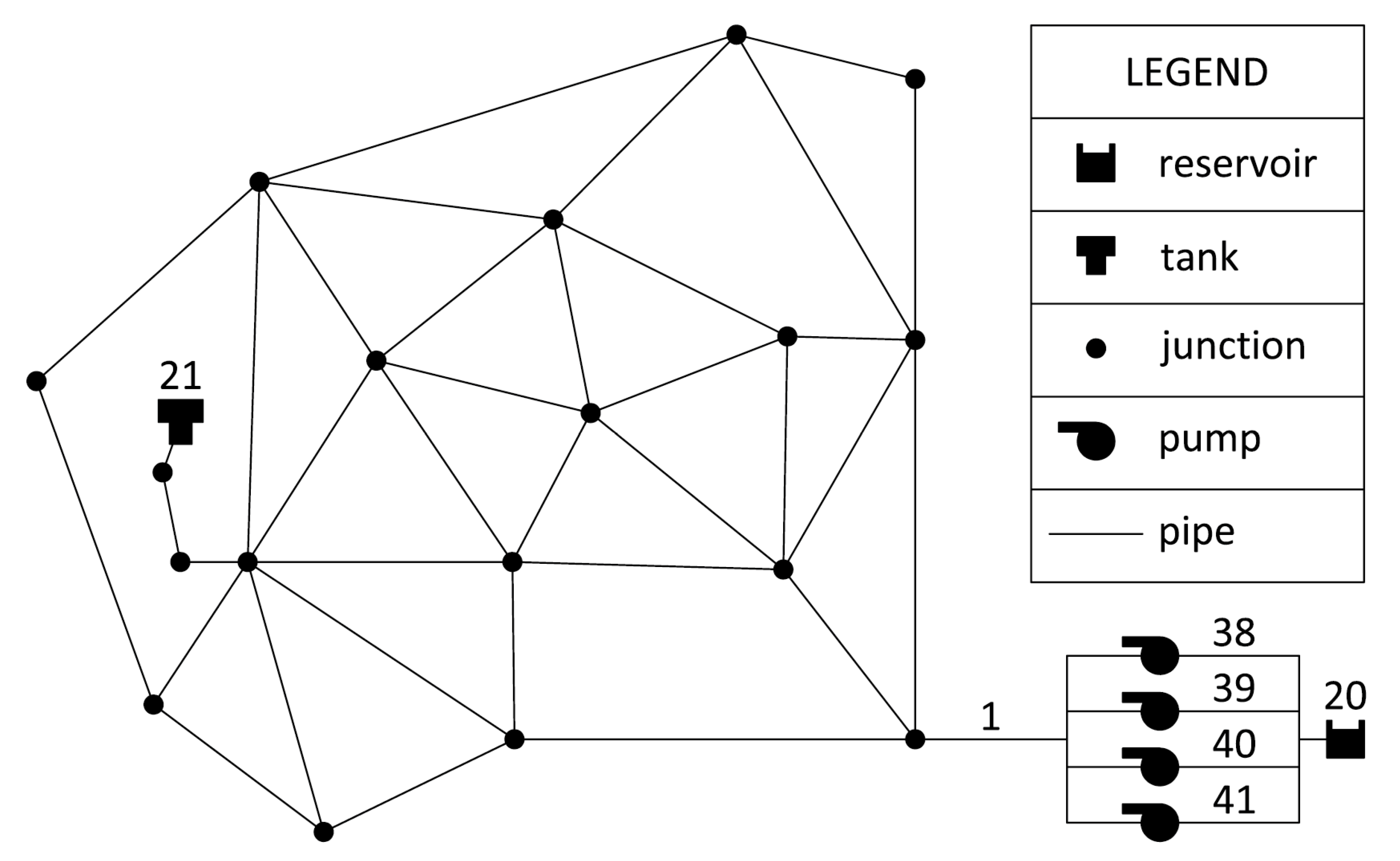
Savic et al. [39] developed a pump scheduling methodology using GA as optimization algorithm and assigning an operation pattern to each pump. In addition to a pattern time-step equal to 1 h, with decision variables assuming the value 0 or 1 for each pattern time-step for each pump, these authors also considered constraint Equations (2)–(4) on the water level in the tank as well as a constraint on the flow that each combination of the pumps can deliver, which is a function of the pump characteristics and the tank water level. They applied the methodology to the case study first analyzed by [47], and subsequently modified by [39], by doubling the original base demand. The WDN is a version of the network usually called Anytown, which consists of 37 pipes, 19 nodes, 1 tank (node 21) and 1 source (node 20). Four pumps are installed at the source, as shown in the network model in Figure 1. The tank elevation and diameter are 215 ft and 40 ft, respectively, with the tank level being the variable between the minimum of 7 ft and the maximum of 35 ft. The energy cost is 0.0244 $/kWh from 00:00 to 07:00 h and 0.1194 $/kWh from 07:00 to 24:00 h. Each pump has its head-discharge curve and efficiency curve. The hydraulic time-step (Δth) is assumed equal to 1 h.
Given this scenario, the best solution was found by assuming the number of maximum total switches is equal to 8, identifies all pumps being switched-on at 00:00 h and running as follows: Pump 38 runs continuously over 24 h; Pump 39 runs continuously for 20 h; Pump 40 runs continuously for 8 h; and Pump 41 runs discontinuously for two hours, from 00:00 to 01:00 h and from 20:00 to 21:00 h. The resulting total cost is $1262.75.
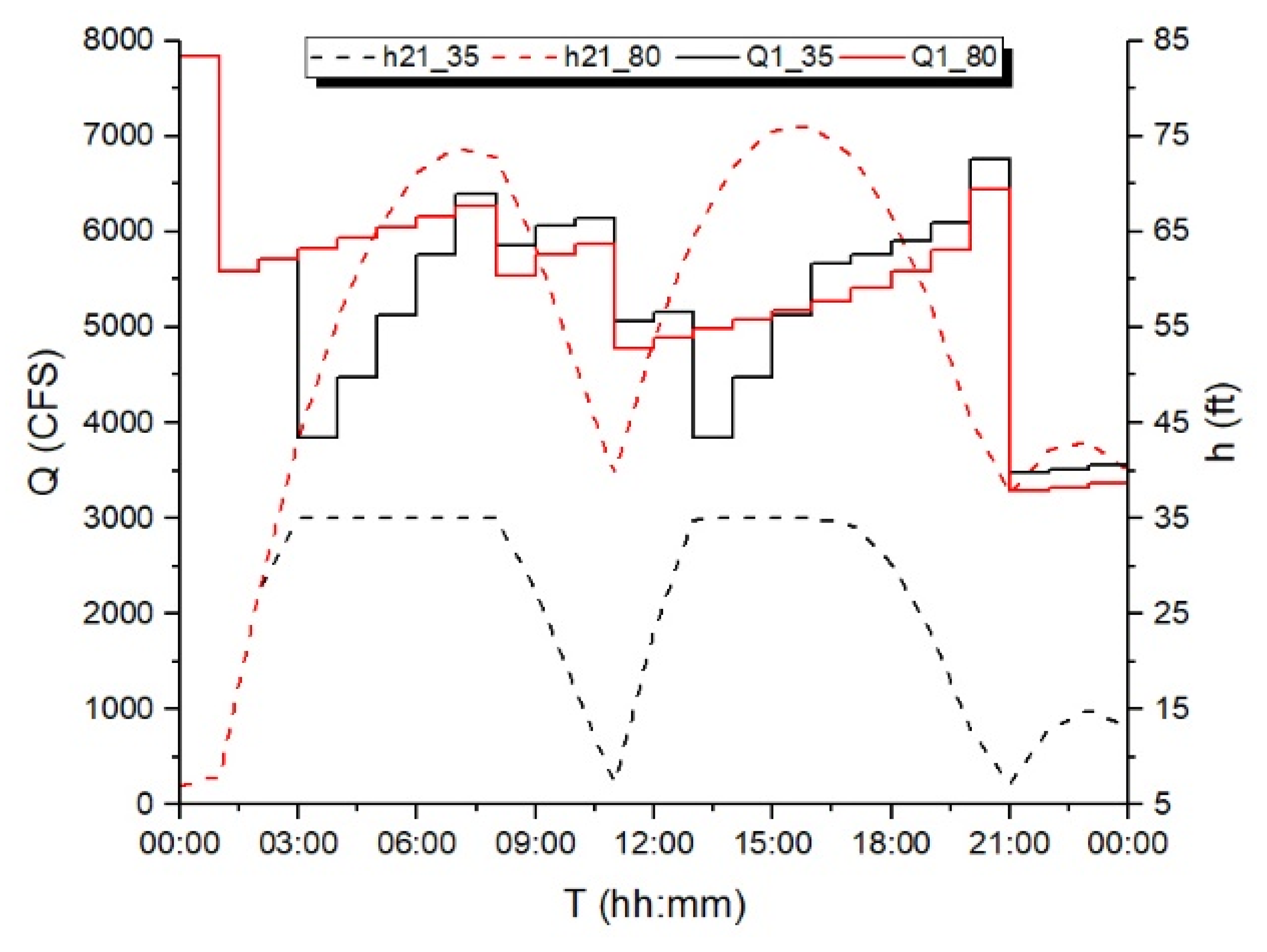
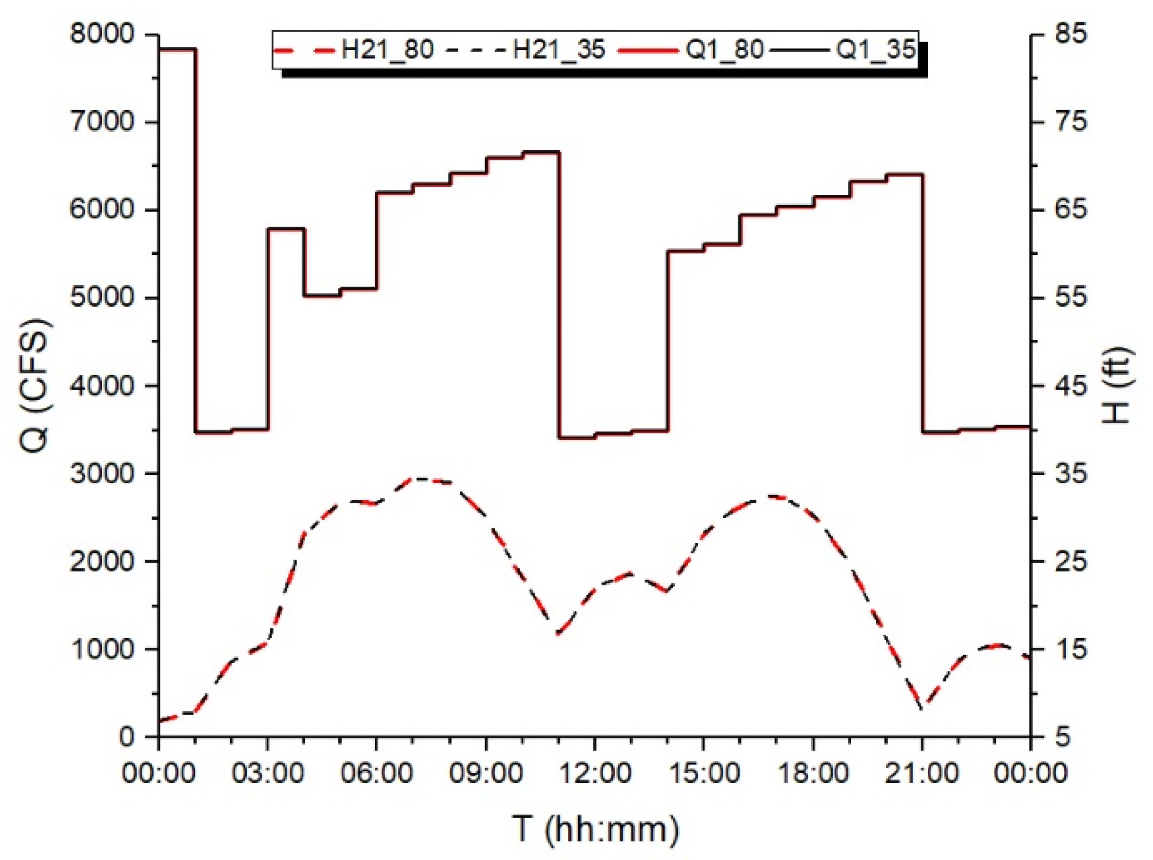
Figure 2 shows the total flow delivered by the pumps, i.e., the flow through conduit 1 (Q1_35) and the water level in the Tank 21 (H21_35). The number 35 in the name of the variables indicates that the maximum allowable tank water level is equal to 35 ft. Total flow varies between 3475 and 7836 CFS and the tank level varies between 7 and 35 ft, thus all constraints are satisfied: the water level is greater than (or equal to) the minimum (7 ft), lower than (or equal to) the maximum (35 ft), and the final value (13.1 ft) is greater than the initial value (7 ft).
In order to assess the effectiveness and reliability of the solution, the optimal pattern resulting from the optimization algorithm was assigned to a new WDN having the same characteristics as the original one except for the maximum tank water level, which is assumed equal to 80 ft. This constraint, using the optimization algorithm-derived pattern, was satisfied (maximum level in the tank was 35 ft), as plotted in Figure 2. In theory, the operation of the system should remain unaltered by this change since it only affects the maximum allowable water level of the tank. Nevertheless, in actual fact the change is found to significantly alter system operation: Figure 2 shows the flow through conduit 1 (Q1_80) and the water level in the Tank 21 (H21_80) being significantly different from the original values (Q1_35 and H21_35). In particular, the tank water level far exceeds the real maximum allowable level (35 ft), reaching the value of 76.1 ft. This example shows the operation pattern determined to be the optimal solution, actually failing to bring about the expected system behavior. From an analytical perspective, the constraint Equation (3) is not satisfied, which would cause the overflow of water from the tank.
3.2. Triggering Based Approach
Marchi et al. [10] developed a pump-scheduling methodology linking Epanet2 [33] with an evolutionary algorithm, and managing operation of pumps by means of Epanet2 rule-based controls. Such controls allow for simultaneously taking into account several conditions (e.g., time of day and tank level) for pump switch-on and switch-off. These authors also introduced a modification in the original Epanet2 libraries in order to better manage rule-based controls and solve the issue arising in calculating energy consumption when rule-based controls are used.
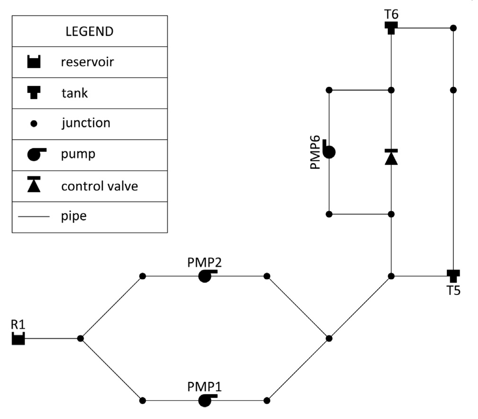
The methodology was applied to the network first introduced by [48]. As plotted in Figure 3, the network consists of 15 pipes and 13 nodes, 2 tanks (T5 and T6) and 1 source (R1) with three pumps installed: two in parallel (PMP1 and PMP2), and a single pump (PMP6). Tank T5 has: elevation of 80 m, diameter of 25 m, minimum and maximum water levels respectively equal to 0 and 5 m; tank T6 has: elevation of 85 m, diameter of 25 m, minimum and maximum water levels respectively equal to 0 and 10 m.
The energy cost is 0.0244 £/kWh from 00:00 to 07:00 h and 0.1194 £/kWh from 07:00 to 24:00 h. Each pump has its own head-discharge curve and efficiency curve. Additional information about system characteristics can be found in the original paper [48].
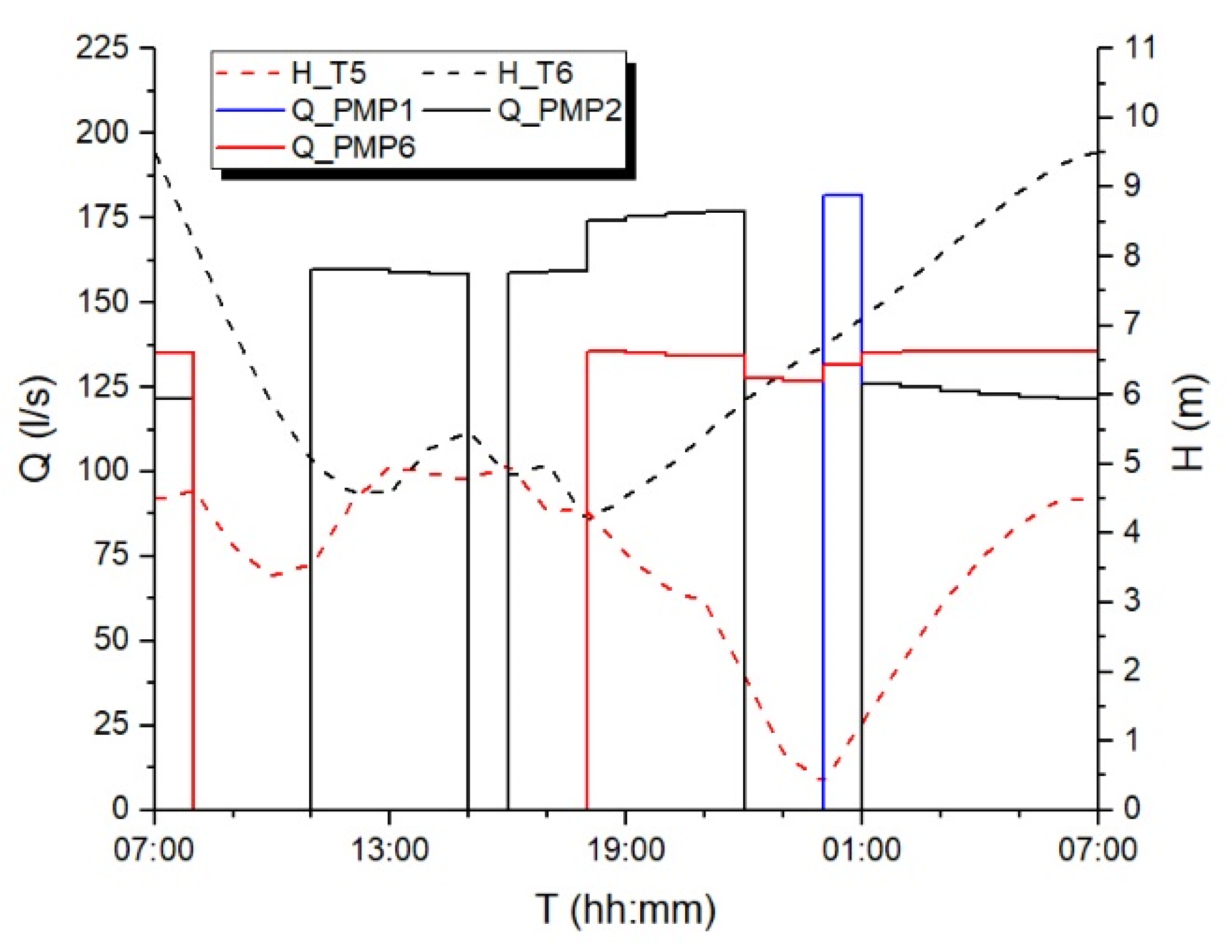
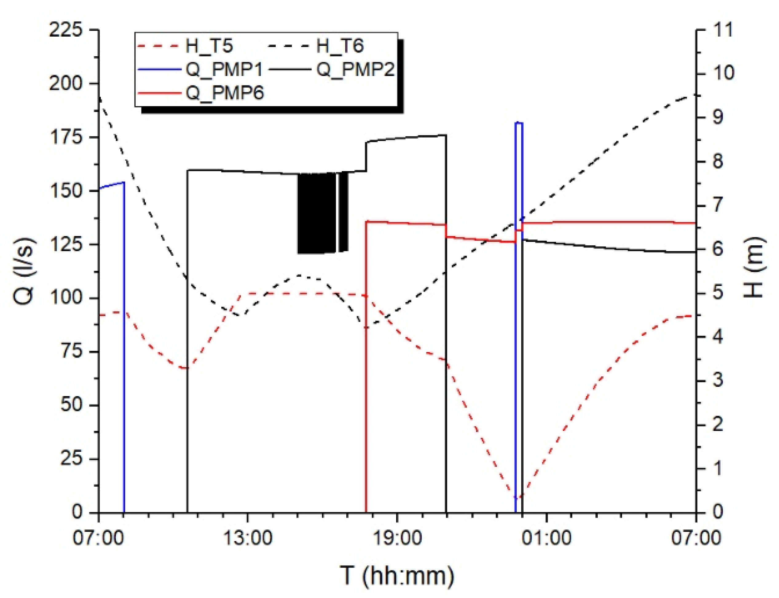
The methodology proposed five solutions, according to the dependence between pump operation and tank water level. Analyzed here below is the solution called Case 2, in which pump PMP1 operates as a function of tank T5 water level, whereas pumps PMP2 and PMP6 operate as a function of tank T6 water level. The hydraulic time-step used in the model was set equal to 1 h, resulting in a total cost of 337.66 £/day. Figure 4 shows the flow delivered by each pump (Q_PMP1, Q_PMP2 and Q_PMP6) and the water level of tanks T5 and T6 (H_T5 and H_T6).
The pumps operate for 8, 17 and 14 h, respectively. The water level in tank T5 varies between 0.40 m and 4.99 m, and the value at the end of simulation coincides with the initial value (4.50 m). For tank T6, the water level varies between 4.18 and 9.52 m, which was also the final value. This value is slightly greater than the initial value (9.50 m).
In order to assess the effectiveness and reliability of the optimal solution, the same rule-based controls were assigned to a new network file, which corresponds to the original model except for the hydraulic time-step, which was set to 10 s instead of 1 h. Reducing the hydraulic time-step enables checking whether or not the operation predicted by the methodology implemented with a larger time-step (1 h) is stable. The resulting system operation may actually differ from the one predicted using a 1-h time-step, in particular when pumps are present in the WDN. A more accurate simulation can be carried out using a smaller hydraulic time-step, albeit at the cost of greater computational effort.
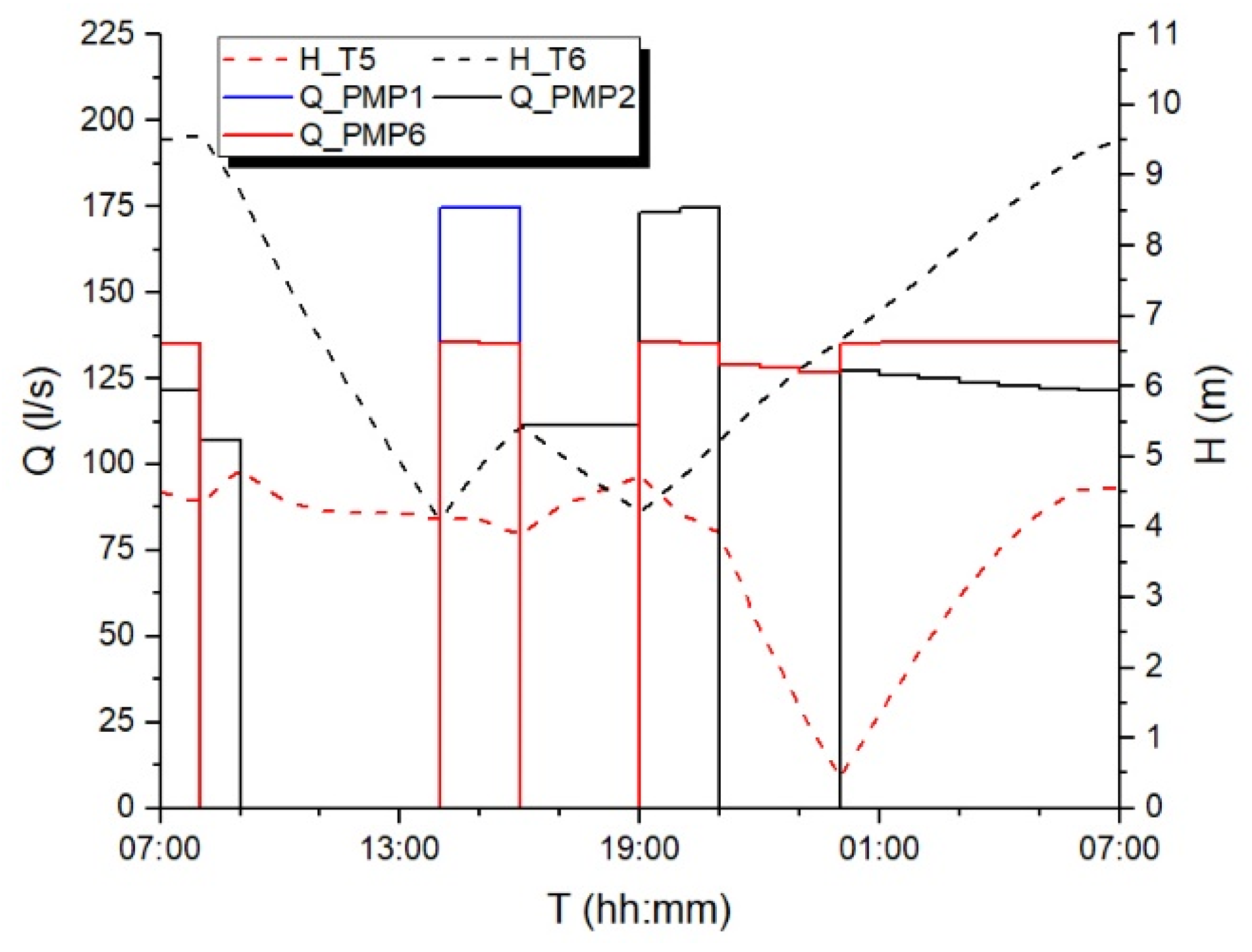
The simulation shows (Figure 5) that in the time interval from 15:00 to 17:00 h, PMP2 is the only operating pump, with a continuously varying pumped flow. That occurs because the level of tank T5 reaches the maximum (5.0 m) and Epanet2 automatically closes the pipe supplying tank T5, being unable to simulate a tank overflow. Consequently, the flow continuously switches between a high value (i.e., the flow required to supply tank T5 and satisfy nodal demands) and a low value (i.e., the flow required to satisfy nodal demands). In real operation, the tank T5 would overflow, since pump PMP2 operates according to trigger-based rules at tank T6. It was found that the optimal operation of pump PMP2 provides for 5.3 m at tank T6 as on-trigger level and 5.5 m as off-trigger level. Because at 15:00 h the water level at tank T6 is 5.42 m and reduces progressively thereafter, pump PMP2 continues operating, and stops only at 20:57 h, when the increasing water level reaches 5.3 m.
The simulation carried out with a reduced hydraulic time-step demonstrates the trigger levels identified as the optimal solution by [10], actually failing to ensure the expected system behavior. As for [39], the constraint Equation (3) not being satisfied would, practically, cause tank T5 to overflow.
4. An Approach to Identify Technically Feasible Solutions
The previous section showed the hydraulic simulation being incapable of simulating the actual operation of the network, whether using a pattern-based approach or a triggering-based approach. The constraint equations were not satisfied, causing in particular, tank overflow. Obviously, that depends on the hydraulic simulation model: significantly reducing the hydraulic time-step (i.e., from 1 h to 1 s) would yield reliable results from the optimization algorithms. However, such an approach is impractical, because it would result in unacceptable computational times.
To avoid such discrepancies, the proposed approach consists in calculating the actual number of time-steps during the simulation and comparing it with the predicted value. In an extended period simulation (EPS), both the simulation duration and the hydraulic time-step (Δth) may be set by the user in Epanet2. Once the hydraulic time-step is set, the total number of time-steps in EPS usually corresponds to the ratio between the total duration of simulation and the hydraulic time-step. Nevertheless, time-steps shorter than the hydraulic time-step will occur automatically (thus increasing the number of total time-steps) upon one of the following occurrences (cases): (a) the next output reporting time period arises; (b) a tank becomes empty or full, (c) the next time pattern period arises; and (d) a simple control or rule-based control is activated.
Case (a) can be simply avoided by setting the reporting time-step equal to the hydraulic time-step. Cases (c) and (d) can be easily predicted, because both the operation pattern and the control rules are known a priori. It follows that the hydraulic time-step becomes shorter than the value fixed at the start of the simulation if a tank becomes empty or full. Epanet2 enables determining when the tank empties out or overflows if the simulation runs with a large hydraulic time-step (e.g., 1 h). However, the results of such additional time-steps do not appear in the software output, thus requiring the use of the Epanet Toolkit.
As discussed in the next section, a pump scheduling methodology that monitors the actual number of time-steps was developed, wherein only technically feasible solutions can be selected.
5. Overview of the Proposed Pump Scheduling Model
A pump-scheduling model which combines Pikaia genetic algorithm [34] as the optimization algorithm and Epanet2 [33] as a hydraulic simulator was developed to implement the proposed methodology and avoid technically unfeasible solutions. Epanet2 was used to load input data, assess the feasibility of the potential solutions generated by the GA and estimate any penalties for constraints violation. The decision variables comprised switch-on time and OD for each pump. The maximum number of switches was imposed.
For any water distribution network where demand patterns, initial tank levels, and electricity tariffs are specified, the goal is to find the best pump schedule such that the total costs are minimized while ensuring adequate network service. The model considered only the pump energy costs, and not maintenance costs. The per-unit energy price is based on electricity tariffs (variable during a scheduling period), generally divided into expensive peak and cheaper off-peak electricity rates. The actual amount of energy consumed by a pump depends on several parameters, including flow running the pump, head supplied by the pump, and pump efficiency. These parameters were calculated by Epanet2 for any assigned pump schedule.
5.1. Decision Variables
For each pump, the initial status (IS) was set on closed and the decision variables were the switch-on times and the OD for each switch. As an example, let be a non-negative real number representing the dimensionless switch-on time of a pump . The daily time in which the pump switches on (SonT) can be defined as:
in which SD is the simulation duration.
A scheduling time-step Δts can also be defined, i.e., the time resolution based on which the pump operating times are set. The scheduling time-step should not be confused with the hydraulic simulation time-step, as will be further discussed. By assuming a daily simulation (i.e., SD = 24 h = 1440 min), the switch-on time becomes:
if Δts is expressed in minutes. Similarly, the pump OD can be calculated as:
x2 being a non-negative real number , with the resulting switch-off time:
In a problem with Np pumps and Ns switches for each pump, the NDV is:
5.2. Objective Function and Constraints
The objective function must take into account the pump operation costs. Since only the cost of energy for pumping is considered, the objective function is given by Equation (1). The constraint equations referring to the water level in the tank also corresponded to previously given Equations (2)–(5).
5.3. Hydraulic Solver and Pumping Operation Model
Epanet 2.0 was used for data input and as a hydraulic solver within the optimization algorithm. The Epanet Toolkit dll was used to incorporate the Epanet functions into the optimization algorithm. Simple control rules were used to assign switch-on and switch-off times of pumps.
Because a single simple control commands switch-on or switch-off time of a pump, for each pump and for each switch, two simple controls are required. Consequently, the proposed model uses a couple of simple controls, one containing SonT and the other SoffT, both calculated according to Equations (7) and (9). By varying the decision variables (SonT and OD), the optimization algorithm minimizes the cost of energy of the pumps.
5.4. Penalty for Technically Unfeasible Solutions
As discussed above, the Epanet Toolkit allows for the monitoring of the number of time-steps when Epanet2 is used as hydraulic simulator. If no additional time-steps occur, or they occur at switch-on or switch-off times commanded by controls, the software continues the calculation of the objective function. Otherwise, a penalty is added to the objective function upon the emptying/overflowing of a tank. This approach enables the actual operation to be reliably simulated without reducing the hydraulic time-step, thus without increasing the computational times.
5.5. Optimization Algorithm
The optimization algorithm uses Pikaia Genetic Algorithm [34]. Pikaia is a flexible and easy to use genetic algorithm written in Fortran 77 and available in the public domain. As with all GAs, the Pikaia genetic algorithm is based on the search for an optimum using Darwinian evolutionary theory. Although its application has been more frequent in astrophysics, it is adaptable for use in a wide variety of modeling applications. The algorithm is based on six steps: initial population generation, fitness evaluation, selection, crossover, mutation, replacement and evaluation. Internally, the algorithm seeks to maximizes a user-specified function f(x) by varying the decision variables. These are randomly generated in the bounded space [0, 1]; therefore, the input parameters must be rescaled.
6. Case Studies and Discussion
The proposed model was applied to the two aforementioned case studies: the Anytown network with the methodologies developed by [39]; and the Van Zyl network with the methodology developed by [10].
For the Anytown WDN consisting of 37 pipes, 19 nodes, 1 tank (node 21), and 1 source (node 20) having four pumps installed (Figure 1), the proposed approach was returned as optimal pump scheduling with 16 simple controls, commanding switch-on and switch-off of the pumps. The solution cost, totaling $1110.32, is cheaper than the original solution found by [39].
Figure 6 shows the total flow delivered by the pumps, i.e., the flow through conduit 1 (Q1_35), ranging between 3416 CFS and 7836 CFS, and the water level in the Tank 21 (H21_35), which ranges between 7 and 34.6 ft. All constraints were respected: the water level did not reach minimum or maximum levels, and the final value (14.0 ft) was greater than the initial value (7 ft).
The effectiveness and reliability of the solution were tested by setting the maximum tank water level to 80 ft. The results are plotted in Figure 6 in terms of total flow through conduit 1 (Q1_80) and the water level in tank 21 (H21_80), which overlaps the curve obtained for 35 ft the maximum allowable level.
For this case study, the proposed approach effectively averts the problem highlighted in Section 3: modifying the maximum level of the tank induced no change in the overall behavior of the system avoiding the overflow of the tank. Therefore, the solution identified as optimal with the proposed approach is cheaper and actually technically feasible as compared to the original solution obtained by [39], which induces tank overflow. Using an Intel Core i5 @2.7GHz personal computer, the model generated a solution after approximately 34 s; yielding the cheapest solution mentioned above after approximately 3.2 h, and a solution with a 5% higher cost after approximately 20 min.
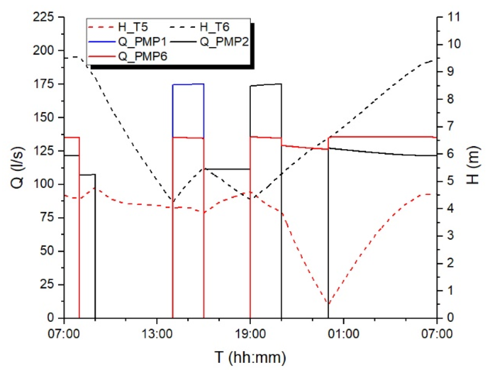
As for the Van Zyl proposed WDN consisting of 15 pipes and 13 nodes, 2 tanks and 1 source, with two pumps installed in parallel, and a single pump (Figure 3), the model returned 12 simple controls, with a solution cost of £341.09—more expensive than the original solution by [10]. In the optimal solution, pumps PMP1 and PMP2 operate for 14 h, pump PMP6 for 15 h. Figure 7 shows the tank T5 water level varying between 0.43 and 4.72 m, with the value at the end of simulation (4.56 m) being slightly greater than the initial value (4.50 m). The water level in the tank T6 starts from 9.50 m, with a minimum of 4.12 m and a maximum of 9.51 m, this value being attained at the end of the simulation; all constraints were thus satisfied.
In order to test the feasibility of proposed approach, the hydraulic time-step was reduced from 1 h to 10 s. The results of flow discharge ran through the pumps (Q_PMP1, Q_PMP2 and Q_PMP6) and water levels in the tanks (H_T5 and H_T6) coincided with that obtained considering a time-step of 1 h (Figure 8) therefore showing the reliability of the solution.
Additionally, the proposed approach in this case study averts the problem discussed in Section 3 wherein reducing the hydraulic time-step induced no difference. The model returned a feasible solution, as opposed to that obtained by [10], which induced tank overflow. Using, an Intel Core i5 @2.7GHz personal computer the model generated a solution after approximately 9 s; it yielded the cheapest solution mentioned above after approximately 13.8 h, and a solution with a 5% higher cost after approximately 5 min.
7. Conclusions
This paper has shown that the solutions identified as optimal by two existing pump scheduling methodologies in the literature are unfeasible and fail to satisfy the imposed constraints. The analysis of these two prior methodologies further showed that the pumping operation identified as “optimal” by the optimization algorithm would, in the real environment, induce tank overflow or continuous pump switching (turning on/off). Such discrepancies could be avoided by reducing the hydraulic time-step of the numerical model, albeit at the cost of increased computational effort, involving high or even unacceptable calculation times.
Consequently, the paper developed a novel method that avoids technically unfeasible solutions and requires limited computational effort. It can also be easily implemented in existing methodologies available in the literature. The proposed method compares the actual number of time-steps performed by the hydraulic simulator with the predicted value, calculated as the ratio between the simulation duration and the hydraulic time-step. If the actual and predicted number of time-steps coincide, all constraints are satisfied, and a technically feasible solution is identified. Accordingly, additional time-steps indicate emptying and/or overflowing of tank, thus identifying solutions not complying with all the constraints. This approach advantageously enables operating with large hydraulic time-steps, thereby supporting reduced computational time-steps.
The effectiveness of the proposed methodology was assessed via a pump-scheduling model developed combining the Pikaia genetic algorithm as an optimization algorithm, and Epanet2 as a hydraulic simulator. In implementing the novel method, the model also adds a penalty to the objective function when the actual number of time-steps is greater than the number predicted. The feasibility of the pump scheduling using the proposed approach was tested for two case studies by reducing the time-step and by increasing the maximum tank level. As opposed to methods used in the literature, the same results were obtained, showing that the developed model effectively averts the problem of tank overflow and continuous pump-switching. In conclusion, the proposed methodology was proven to be reliable, and capable of simulating the actual operation of the system.
Author Contributions
Conceptualization, G.M. and N.F.; methodology, G.M. and N.F.; software, M.M. and F.D.M.; validation, G.M., N.F. and M.G.; data curation, M.M. and F.D.M.; writing—original draft preparation, G.M.; writing—review and editing, N.F.; supervision, M.G. All authors have read and agreed to the published version of the manuscript.
Funding
This research was funded by Progetto ARS01_01080 “WATERGY—L’efficientamento energetico del Servizio Idrico Integrato” CUP B52F20001180005.
Data Availability Statement
Some or all data, models, or code that support the findings of this study are available from the corresponding author upon reasonable request.
Conflicts of Interest
The authors declare no conflict of interest.
References
- Dai, J.; Wu, S.; Han, G.; Weinberg, J.; Xie, X.; Wu, X.; Song, X.; Jia, B.; Xue, W.; Yang, Q. Water-Energy Nexus: A Review of Methods and Tools for Macro-Assessment. Appl. Energy 2018, 210, 393–408. [Google Scholar] [CrossRef]
- Bagirov, A.M.; Barton, A.F.; Mala-Jetmarova, H.; al Nuaimat, A.; Ahmed, S.T.; Sultanova, N.; Yearwood, J. An Algorithm for Minimization of Pumping Costs in Water Distribution Systems Using a Novel Approach to Pump Scheduling. Math. Comput. Model. 2013, 57, 873–886. [Google Scholar] [CrossRef]
- Cantu-Funes, R.; Coelho, L.C. Simulation-Based Optimization of Pump Scheduling for Drinking Water Distribution Systems. Eng. Optim. 2022, 1–15. [Google Scholar] [CrossRef]
- Jafari-Asl, J.; Azizyan, G.; Monfared, S.A.H.; Rashki, M.; Andrade-Campos, A.G. An Enhanced Binary Dragonfly Algorithm Based on a V-Shaped Transfer Function for Optimization of Pump Scheduling Program in Water Supply Systems (Case Study of Iran). Eng. Fail. Anal. 2021, 123, 105323. [Google Scholar] [CrossRef]
- Jowitt, P.W.; Germanopoulos, G. Optimal Pump Scheduling in Water-Supply Networks. J. Water Resour. Plan. Manag. 1992, 118, 406–422. [Google Scholar] [CrossRef]
- Chase, D.v.; Ormsbee, L.E. Computer-Generated Pumping Schedules for Satisfying Operational Objectives. J. Am. Water Works Assoc. 1993, 85, 54–61. [Google Scholar] [CrossRef]
- Lansey, K.E.; Awumah, K. Optimal Pump Operations Considering Pump Switches. J. Water Resour. Plan. Manag. 1994, 120, 17–35. [Google Scholar] [CrossRef]
- Nitivattananon, V.; Sadowski, E.C.; Quimpo, R.G. Optimization of Water Supply System Operation. J. Water Resour. Plan. Manag. 1996, 122, 374–384. [Google Scholar] [CrossRef]
- Castro-Gama, M.; Pan, Q.; Lanfranchi, E.A.; Jonoski, A.; Solomatine, D.P. Pump Scheduling for a Large Water Distribution Network. Milan, Italy. In Procedia Engineering; Elsevier Ltd.: Amsterdam, The Netherlands, 2017; Volume 186, pp. 436–443. [Google Scholar]
- Marchi, A.; Simpson, A.R.; Lambert, M.F. Optimization of Pump Operation Using Rule-Based Controls in EPANET2: New ETTAR Toolkit and Correction of Energy Computation. J. Water Resour. Plan. Manag. 2016, 142, 04016012. [Google Scholar] [CrossRef] [Green Version]
- Cimorelli, L.; Fecarotta, O. Optimal Regulation of Variable Speed Pumps in Sewer Systems. In Proceedings of the 4th EWaS International Conference: Valuing the Water, Carbon, Ecological Footprints of Human Activities, Kerkira, Greece, 24–27 June 2020; p. 58. [Google Scholar]
- Luna, T.; Ribau, J.; Figueiredo, D.; Alves, R. Improving Energy Efficiency in Water Supply Systems with Pump Scheduling Optimization. J. Clean. Prod. 2019, 213, 342–356. [Google Scholar] [CrossRef]
- Maskit, M.; Ostfeld, A. Multi-Objective Operation-Leakage Optimization and Calibration of Water Distribution Systems. Water 2021, 13, 1606. [Google Scholar] [CrossRef]
- Shao, Y.; Yu, Y.; Yu, T.; Chu, S.; Liu, X. Leakage Control and Energy Consumption Optimization in the Water Distribution Network Based on Joint Scheduling of Pumps and Valves. Energies 2019, 12, 2969. [Google Scholar] [CrossRef] [Green Version]
- Goldberg, D.E. Genetic and Evolutionary Algorithms Come of Age. Commun. ACM 1994, 37, 113–120. [Google Scholar] [CrossRef]
- Goldberg, D.E. Genetic Algorithms in Search, Optimization, and Machine Learning; Addison: Boston, MA, USA, 1989. [Google Scholar]
- Georgescu, S.C.; Georgescu, A.M. Application of HBMOA to Pumping Stations Scheduling for a Water Distribution Network with Multiple Tanks. In Procedia Engineering; Elsevier Ltd.: Amsterdam, The Netherlands, 2014; Volume 70, pp. 715–723. [Google Scholar]
- Abdelsalam, A.A.; Gabbar, H.A. Energy Saving and Management of Water Pumping Networks. Heliyon 2021, 7, e07820. [Google Scholar] [CrossRef]
- Xin, S.; Liang, Y.; Zhou, X.; Li, W.; Zhang, J.; Song, X.; Yu, C.; Zhang, H. A Two-Stage Strategy for the Pump Optimal Scheduling of Refined Products Pipelines. Chem. Eng. Res. Des. 2019, 152, 1–19. [Google Scholar] [CrossRef]
- Fecarotta, O.; Carravetta, A.; Morani, M.; Padulano, R. Optimal Pump Scheduling for Urban Drainage under Variable Flow Conditions. Resources 2018, 7, 73. [Google Scholar] [CrossRef] [Green Version]
- Gao, J.; Qi, S.; Wu, W.; Han, A.; Chen, C.; Ruan, T. Leakage Control of Multi-Source Water Distribution System by Optimal Pump Schedule. In Procedia Engineering; Elsevier Ltd.: Amsterdam, The Netherlands, 2014; Volume 70, pp. 698–706. [Google Scholar]
- Dai, P.D.; Viet, N.H. Optimization of Variable Speed Pump Scheduling for Minimization of Energy and Water Leakage Costs in Water Distribution Systems with Storages. In Proceedings of the 13th International Conference on Electronics, Computers and Artificial Intelligence, ECAI 2021, Pitesti, Romania, 1–3 July 2021; Institute of Electrical and Electronics Engineers Inc.: Piscataway, NJ, USA, 2021. [Google Scholar]
- Soleimani, B.; Keihan Asl, D.; Estakhr, J.; Seifi, A.R. Integrated Optimization of Multi-Carrier Energy Systems: Water-Energy Nexus Case. Energy 2022, 257, 124764. [Google Scholar] [CrossRef]
- Moazeni, F.; Khazaei, J. Optimal Energy Management of Water-Energy Networks via Optimal Placement of Pumps-as-Turbines and Demand Response through Water Storage Tanks. Appl. Energy 2021, 283, 116335. [Google Scholar] [CrossRef]
- Darweesh, M.S. Impact of Optimized Pump Scheduling on Water Quality in Distribution Systems. J. Pipeline Syst. Eng. Pract. 2020, 11, 05020004. [Google Scholar] [CrossRef]
- Choi, Y.H. Development of Optimal Water Distribution System Design and Operation Approach Considering Hydraulic and Water Quality Criteria in Many-Objective Optimization Framework. J. Comput. Des. Eng. 2022, 9, 507–518. [Google Scholar] [CrossRef]
- Ayyagari, K.S.; Gatsis, N. Optimal Pump Scheduling in Multi-Phase Distribution Networks Using Benders Decomposition. Electr. Power Syst. Res. 2022, 212, 108584. [Google Scholar] [CrossRef]
- Zanoli, S.M.; Astolfi, G.; Orlietti, L.; Frisinghelli, M.; Pepe, C. Water Distribution Networks Optimization: A Real Case Study. In IFAC-PapersOnLine; Elsevier: Amsterdam, The Netherlands, 2020; Volume 53, pp. 16644–16650. [Google Scholar]
- Carricondo-Antón, J.M.; Jiménez-Bello, M.A.; Manzano Juárez, J.; Royuela Tomas, A.; Sala, A. Evaluating the Use of Meteorological Predictions in Directly Pumped Irrigational Operations Using Photovoltaic Energy. Agric. Water Manag. 2022, 266, 107596. [Google Scholar] [CrossRef]
- Naval, N.; Yusta, J.M. Optimal Short-Term Water-Energy Dispatch for Pumping Stations with Grid-Connected Photovoltaic Self-Generation. J. Clean. Prod. 2021, 316, 128386. [Google Scholar] [CrossRef]
- Zavala, V.; López-Luque, R.; Reca, J.; Martínez, J.; Lao, M.T. Optimal Management of a Multisector Standalone Direct Pumping Photovoltaic Irrigation System. Appl. Energy 2020, 260, 114261. [Google Scholar] [CrossRef]
- Mérida García, A.; Fernández García, I.; Camacho Poyato, E.; Montesinos Barrios, P.; Rodríguez Díaz, J.A. Coupling Irrigation Scheduling with Solar Energy Production in a Smart Irrigation Management System. J. Clean. Prod. 2018, 175, 670–682. [Google Scholar] [CrossRef]
- Rossman, L.A. EPANET 2: Users Manual; United States Environmental Protection Agency: Washington, DC, USA, 2000. [Google Scholar]
- Charbonneau, P.; Knapp, B. A User’s Guide to PIKAIA 1.0; University Corporation for Atmospheric Research: Boulder, CO, USA, 1995. [Google Scholar]
- Ngancha, P.B.; Kusakana, K.; Markus, E.D. Optimal Pumping Scheduling for Municipal Water Storage Systems. Energy Rep. 2022, 8, 1126–1137. [Google Scholar] [CrossRef]
- Mackle, G. Application of Genetic Algorithms to Pump Scheduling for Water Supply. In Proceedings of the 1st International Conference on Genetic Algorithms in Engineering Systems: Innovations and Applications (GALESIA), IEE, Sheffield, UK, 12–14 September 1995; pp. 400–405. [Google Scholar]
- Barán, B.; von Lücken, C.; Sotelo, A. Multi-Objective Pump Scheduling Optimisation Using Evolutionary Strategies. Adv. Eng. Softw. 2005, 36, 39–47. [Google Scholar] [CrossRef]
- Salomons, E.; Goryashko, A.; Shamir, U.; Rao, Z.; Alvisi, S. Optimizing the Operation of the Haifa-A Water-Distribution Network. J. Hydroinform. 2007, 9, 51–64. [Google Scholar] [CrossRef] [Green Version]
- Savić, D.A.; Bicik, J.; Morley, M.S. A DSS Generator for Multiobjective Optimisation of Spreadsheet-Based Models. Environ. Model. Softw. 2011, 26, 551–561. [Google Scholar] [CrossRef] [Green Version]
- Ibarra, D.; Arnal, J. Parallel Programming Techniques Applied to Water Pump Scheduling Problems. J. Water Resour. Plan Manag. 2014, 140, 06014002. [Google Scholar] [CrossRef]
- de Paola, F.; Fontana, N.; Giugni, M.; Marini, G.; Pugliese, F. An Application of the Harmony-Search Multi-Objective (HSMO) Optimization Algorithm for the Solution of Pump Scheduling Problem. Procedia Eng. 2016, 162, 494–502. [Google Scholar] [CrossRef] [Green Version]
- de Paola, F.; Fontana, N.; Giugni, M.; Marini, G.; Pugliese, F. Optimal Solving of the Pump Scheduling Problem by Using a Harmony Search Optimization Algorithm. J. Hydroinform. 2017, 19, 879–889. [Google Scholar] [CrossRef] [Green Version]
- López-Ibáñez, M.; Prasad, T.D.; Paechter, B. Ant Colony Optimization for Optimal Control of Pumps in Water Distribution Networks. J. Water Resour. Plan Manag. 2008, 134, 337–346. [Google Scholar] [CrossRef]
- Brion, L.M.; Mays, L.W. Methodology for Optimal Operation of Pumping Stations in Water Distribution Systems. J. Hydraul. Eng. 1991, 117, 1551–1569. [Google Scholar] [CrossRef]
- Quintiliani, C.; Creaco, E. Using Additional Time Slots for Improving Pump Control Optimization Based on Trigger Levels. Water Resour. Manag. 2019, 33, 3175–3186. [Google Scholar] [CrossRef]
- Alvisi, S.; Franchini, M. A Robust Approach Based on Time Variable Trigger Levels for Pump Control. J. Hydroinform. 2017, 19, 811–822. [Google Scholar] [CrossRef] [Green Version]
- Pasha, M.F.K.; Lansey, K. Optimal Pump Scheduling by Linear Programming. In Proceedings of the World Environmental and Water Resources Congress 2009, Kansas City, MO, USA, 17–21 May 2009; American Society of Civil Engineers: Reston, VA, USA, 2009; pp. 1–10. [Google Scholar]
- van Zyl, J.E.; Savic, D.A.; Walters, G.A. Operational Optimization of Water Distribution Systems Using a Hybrid Genetic Algorithm. J. Water Resour. Plan Manag. 2004, 130, 160–170. [Google Scholar] [CrossRef]
Figure 1.
Anytown water distribution network model [39].
Figure 1.
Anytown water distribution network model [39].

Figure 2.
Results of the pump scheduling model by [39] for Anytown network.
Figure 2.
Results of the pump scheduling model by [39] for Anytown network.

Figure 3.
Van Zyl water distribution network model [48].
Figure 3.
Van Zyl water distribution network model [48].

Figure 4.
Results of the pump scheduling methodology by [10] for Van Zyl network, hydraulic time-step 1 h.
Figure 4.
Results of the pump scheduling methodology by [10] for Van Zyl network, hydraulic time-step 1 h.

Figure 5.
Results of the pump scheduling methodology by [10] for Van Zyl network, hydraulic time-step 10 s.
Figure 5.
Results of the pump scheduling methodology by [10] for Van Zyl network, hydraulic time-step 10 s.

Figure 6.
Results of the proposed pump scheduling methodology for Anytown network.

Figure 7.
Results of the proposed pump scheduling methodology for Van Zyl network, hydraulic time-step 1 h.
Figure 7.
Results of the proposed pump scheduling methodology for Van Zyl network, hydraulic time-step 1 h.

Figure 8.
Results of the proposed pump scheduling methodology for Van Zyl network, hydraulic time-step 10 s.
Figure 8.
Results of the proposed pump scheduling methodology for Van Zyl network, hydraulic time-step 10 s.

Disclaimer/Publisher’s Note: The statements, opinions and data contained in all publications are solely those of the individual author(s) and contributor(s) and not of MDPI and/or the editor(s). MDPI and/or the editor(s) disclaim responsibility for any injury to people or property resulting from any ideas, methods, instructions or products referred to in the content. |
© 2023 by the authors. Licensee MDPI, Basel, Switzerland. This article is an open access article distributed under the terms and conditions of the Creative Commons Attribution (CC BY) license (https://creativecommons.org/licenses/by/4.0/).
Share and Cite
MDPI and ACS Style
Marini, G.; Fontana, N.; Maio, M.; Di Menna, F.; Giugni, M. A Novel Approach to Avoiding Technically Unfeasible Solutions in the Pump Scheduling Problem. Water 2023, 15, 286. https://doi.org/10.3390/w15020286
AMA Style
Marini G, Fontana N, Maio M, Di Menna F, Giugni M. A Novel Approach to Avoiding Technically Unfeasible Solutions in the Pump Scheduling Problem. Water. 2023; 15(2):286. https://doi.org/10.3390/w15020286
Chicago/Turabian StyleMarini, Gustavo, Nicola Fontana, Marco Maio, Francesco Di Menna, and Maurizio Giugni. 2023. "A Novel Approach to Avoiding Technically Unfeasible Solutions in the Pump Scheduling Problem" Water 15, no. 2: 286. https://doi.org/10.3390/w15020286
Note that from the first issue of 2016, this journal uses article numbers instead of page numbers. See further details here.