Hydro-Environmental Sustainability of Crop Production under Socioeconomic Drought

Abstract

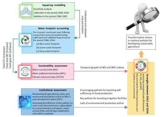
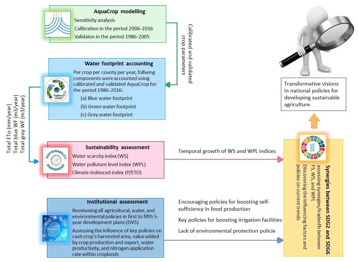
A comprehensive framework for revealing the jeopardization between SDGs 2 and 6 is provided in this study. Along with a water footprint (WF) assessment, the 30-years pattern of agricultural WFs and its hydro-environmental, social, and ecopolitical (SEP) consequences were quantified for the major food producer regions of Iran, as it is a water-bankrupted country under socioeconomic drought. In addition, the enforced impacts of major water/food-related policies on environmental sustainability were analyzed through an institutional assessment. During 1986–2016, BWS and GWD raised with annual average rates of 5% and 44%, respectively. Consequently, SEP status prospered along with an 18% increase in irrigated area, 198% in added-value by crop production and 5% by staple-crop exports, and 51% in the number of agricultural workers. The Pearson correlation analysis revealed a significant tradeoff between self-supplied food availability and SEP. A 54% increase in food production occurred at the cost of 80% overexploitation in blue water resources and quality degradation. An annual average increase of 1.1% in P/ETo indicates the dominant role of anthropogenic interventions in such deteriorations. The institutional assessment demonstrated that environmental sustainability policies have never been applied as promoting policies to boost self-sufficiency in food production. According to the results, hydrological sustainability requires a transformative vision in national policies to exploit limited water and soil resources while preserving the environment.

1. Introduction

In 2015, the United Nations General Assembly adopted 17 sustainable development goals (SDGs), which are supposed to be achieved by 2030. While addressing different pillars (i.e., socioeconomic development and environmental protection), these goals are deeply intertwined and should be implemented in an indivisible framework [1]. Indeed, separate persuasion of one goal may cause losing the other ones. For instance, progress towards ending hunger (SDG 2) over the past decades almost occurred at the cost of unsustainable water consumption and pollution, which is against SDG 6 (i.e., clean water and sanitation). Target 6.3 under SDG 6 denotes that water quality should be improved by reducing pollution in water bodies by 2030. On the other hand, target 6.4 emphasizes on reducing the number of people who face blue water scarcity in the world. However, human appropriation of freshwater resources caused the number of people who face severe water scarcity at least one month of a year to increase to four billion people in the world [2]. On the other hand, nitrogen assimilation capacity of freshwater resources is exceeded in 17% of the world’s land area where 48% of global population are living. Such pollution is mainly caused by the excessive application of nitrogen in agricultural lands [3,4,5,6]. Phosphorous applications also caused P-related grey water footprint to exceed a basin’s assimilation capacity in 38% of land area in the world that contributes 37% in global river discharge and is occupied by 90% of the global population [7]. Cereals contribute the most either in nitrogen or in phosphorous load to water bodies in the world [8].

While reconciling food security in the world jeopardized SDG 6, the statistics reported by FAO also demonstrate that the SDG 2 indicators are not properly met. Based on the FAO report on the status of food security and nutrition in the world, the number of people who experienced food insecurity (moderately or severely) increased by 44%, from 1645.5 million in 2014 to 2368.2 million in 2020. In addition, the prevalence of moderate or severe food insecurity increased from 22.6% in 2014 to 30.4% in 2020 [9]. Such results indicate that there is still limited understanding of potential tradeoffs and synergies between different SDGs.

Countries behaved differently to address such coherences. For instance, half of the people who face water scarcity are living in China and India [2]; however, the government of these two countries adopted a different approach to address food security challenges [10]. During 2002–2007, China’s net virtual water (VW) export increased by 75% from 39 to 68 billion m³ y⁻¹. While such international trade pattern improved the economic status of the country, it caused the ratio of net VW exports to local water availability in water-scarce North-China to increase from 3.6% to 5.1%, which resulted in exacerbating water scarcity status there [11]. From 2012–2018, however, the government launched several national policies, all of which emphasized the sustainable development of agriculture and water resource management. These policies, which included increasing the number of trading partners for importing water-intensive crops, supporting sustainable agriculture, following land conservation targets, and reducing groundwater consumption, resulted in a considerable reduction in environmental deterioration in China [12,13]. In contrast, India is still supplying its domestic food demand within the nation, and only 3% of its water footprint (WF) locates out of the county [14]. The inter-state VW flow direction is from water scarce regions to water-abundant ones, which caused most of the northern states to be under red zone due to groundwater overexploitation [15]. Indeed, VW flow direction is mainly dictated by per capita harvested area and access to a secured market rather than by water endowment in India. Economic interests caused the country to be a net VW exporter as well, resulting in the exacerbation of water scarcity. Nevertheless, water-related issues do not place at the top of the political agenda in India. While Indian irrigation water use is 83% higher than one in the rest of the world, the government has not planned to improve irrigation water use efficiency yet.

Iran is also among the countries with severe water scarcity and environmental deterioration challenges. Karandish [16] reported that the entire country faces severe water scarcity during May-September period. The agricultural sector in this country represents more than 90% of the total freshwater use [17]. Roughly 71% of Iranians live in areas which are at high risk of land subsidence due to groundwater overexploitation. Such overexploitations mainly occurred in the agricultural sector, which is stressed by the government to assure Iran’s self-sufficiency in food production. A consequence of Iran’s food self-sufficiency policy was the exhaustion of water resources in rural areas and the consequent climate-migration of rural residents to the surrounding cities, resulting in the intensification of water shortage in capitals.

Recently, an ongoing farmers’ protest formed against water shortage, particularly in areas like Khuzestan province, which are the backbones of Iran’s agriculture. Possessing 30% of national surface water resources, Khuzestan supplies 14% and 62% of total cereals and sugar crops productions in Iran, respectively [18]. Nevertheless, an inefficient and unsustainable water consumption pattern within this province on the one hand and the implementation of inter-basin water transfer projects on the other hand seriously affected farmer’s livelihood and the environment in downstream regions, and it increased tensions between water donating and receiving provinces [19]. Annually, a total of 1.3 billion m³ y⁻¹ water is physically transferred from the Karun and Dez rivers in upstream regions to central water-scarce provinces of Iran, which consequently reduces water flow to Khuzestan province. Such improper policies are not only a threat to Khuzestan’s socioeconomic and environmental structures, but also is a threat to national food security. In addition, major oil exploitation industries are located in Khuzestan province, and, therefore, the water shortage is a great threat to the continuation of these industries’ activities, to which the large share of Iran’s GDP is dependent. It is worth noting that Khuzestan has geopolitical significance as well since it is a border province which shares the Persian Gulf with Iraq. Hence, a lack of proper control over internal conflicts in Khuzestan province can flare international water tensions [20].

Due to the significant geopolitical position of Khuzestan province and its agricultural role in the national economy, we tried to find out possible synergies and/or trade-offs between the main objectives of SDG 2 (zero hunger) in terms of food availability and SDG 6 (clean water and sanitation) in terms of water scarcity in this province. With this aim, we carried out a comprehensive green, blue, and grey WF assessment of the agricultural sector in the Khuzestan province from 1986 to 2016. We made a long-term assessment to analyse how changes in political strategies affected the sustainability and efficiency of water use in the study area. Since Iran’s policy/decision makers are about to write Iran’s 7th 5-years development plan program, the outcomes of this study can help them with implementing a sustainable plan by providing a deep understanding of the main roots of the current socioeconomic and environmental unsustainability in this province, which has been caused through the past 5-year programs.

2. Methods and Data

2.1. Study Area

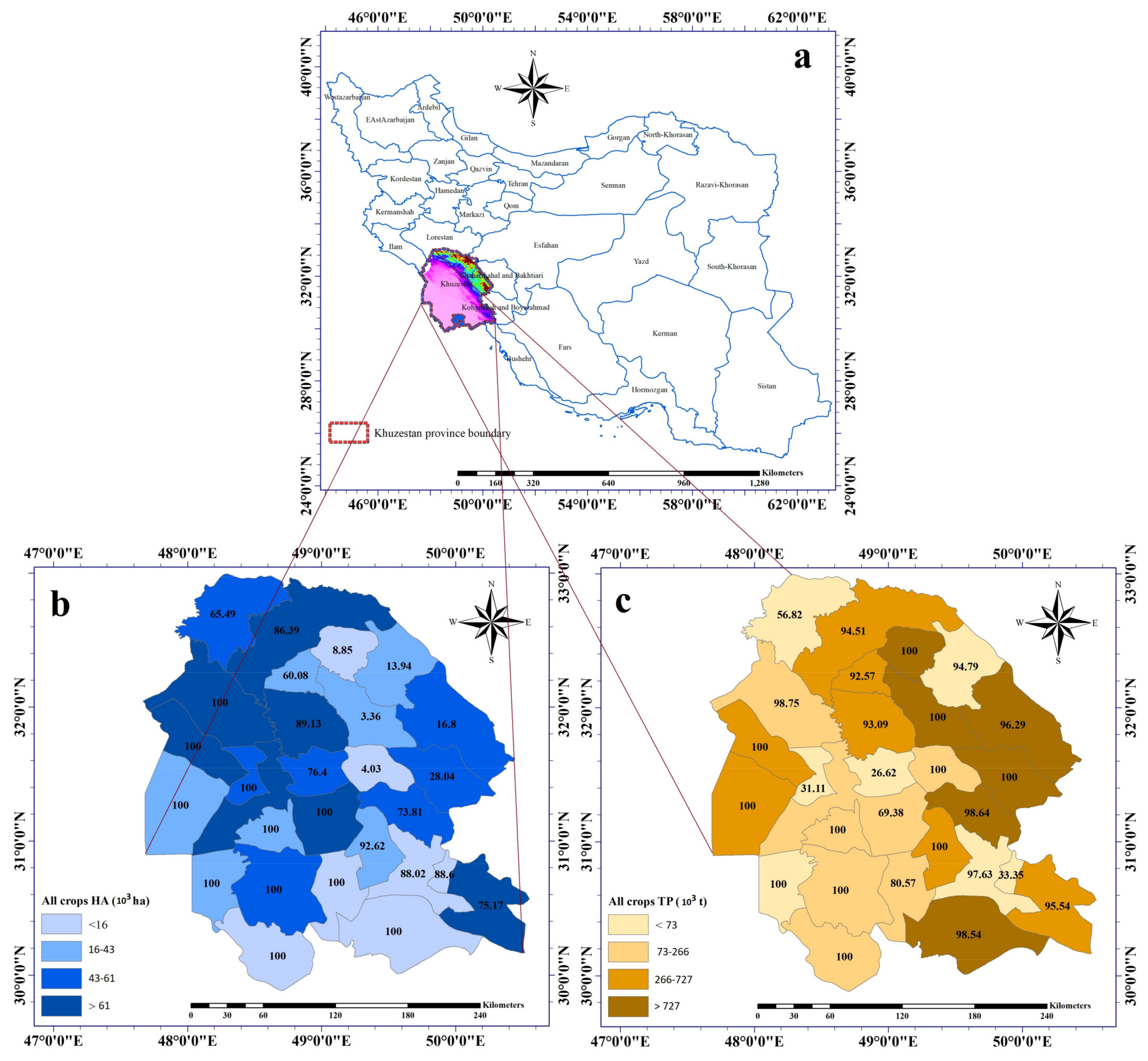
Khuzestan province in the southwest of Iran lies between 29°57′ N to 33°00′ N latitudes and 47°40′ E to 50°33′ E longitudes, and it spans an area of 62,818 Km² (i.e., roughly 4% of Iran’s area) (Figure 1). There are a total of 27 counties in the province with a dominant arid climate condition [20]. Based on the de-Martonne climate classification method, the dominant climate condition in Khuzestan province is an arid climate [5]. The province has only 37 rainy days with an average annual precipitation of 24.8 mm. The average temperature is about 30.24 °C, which is roughly 12% higher than the country average. Long-term annual averages of minimum and maximum temperatures and relative humidity are 24.2 °C, 34.7 °C, and 24%, respectively.

The province possesses about 30% of Iran’s surface water resources and, therefore, is the backbone of Iran’s agriculture. About 9% of Iran’s croplands are located in Khuzestan province, in which 13% of the country’s crops are produced. While 20% of total employees are occupied in the agricultural sector, they only produce 7% of the provincial GDP (i.e., gross domestic production).

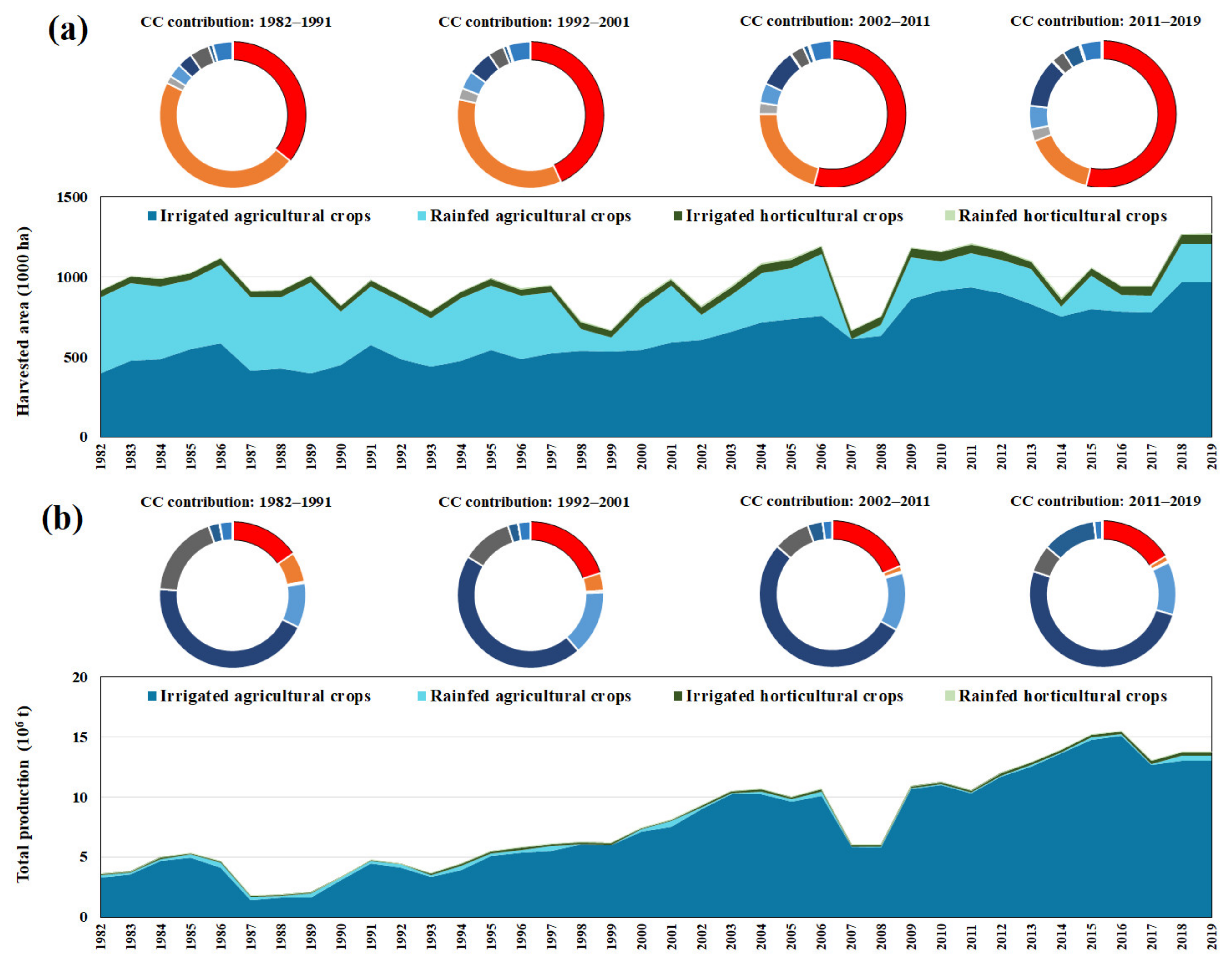
Figure 2 shows the temporal and spatial variation of the harvested area and total production in Khuzestan province over the period 1982–2019 [18]. Along with a 39% increase in the total harvested area (HA) over the study period, the total crop production (TP) increased by 282%. Such a high increase in TP attributes to changes that occurred in the cropping pattens and the highlighted increase in crop’s yield over the study period. Irrigation plays a major role in crop production in the study area. Roughly 99% of the total production in Khuzestan province is supplied from irrigated croplands, which contributes 84% in the total harvested area. While the north and north-east of the province contribute the most in the total harvested area, the eastern parts of the province contribute the most in total crop production since crops with higher yields are cultivated there.

In this study, which was conducted for the period 1986–2016, we selected 32 crops and classified them into 10 groups including cereals, vegetables and melons, root and tuber, sugar crops, temporal oil crops, fodder crops, nuts, permanent oil seeds, (sub-)tropical fruits, and other fruits. Crops under each crop category are summarized in

Table 1. Selected crops under each crop category, and their overall contributions in total harvested area and production in the Khuzestan province over the period 1986–2016.

Crop Category	Selected Crops in the Category	Crop Type	Contribution in Total Harvested Area (%)	Contribution in Total Production (%)
Cereals	Wheat, barley, rice, maize	Staple	73.84	15.04
Vegetables/cucumber-family crops	Tomato, cucumber, onion, melon, watermelon	Staple	6.54	16.33
Fodder crops	Sorghum and alfalfa	Cash	3.93	13.67
Fiber crops	Potato	Staple	0.30	0.40
Tropical/semi-tropical fruits	Date, fig, jujube	Cash	0.16	0.06
Nuts	Walnut	Cash	3.48	1.15
Other fruits	Apple, apricot, peach, grape, orange, grapefruit, sour orange, mandarin, lime, lemon, pomegranate	Cash	0.01	0.01
Temporally oil crops	Canola, sesame	Cash	0.56	0.03
Permanent oil crops	Olive	Cash	0.01	0.01
Sugar crops	Sugar beet, sugar cane	Cash	11.17	53.31

.

2.2. Water Footprint Accounting

2.2.1. AquaCrop Modeling

The AquaCrop model per crop per province was used to simulate the green and blue evapotranspiration (ET). A daily water balance equation is adopted by the AquaCrop model to simulate soil water dynamics as follows [21]:

$$S_{\left[t\right]}=S_{\left[t-1\right]}+P_{\left[t\right]}+I_{\left[t\right]}+C{R}_{\left[t\right]}-E{T}_{\left[t\right]}-R{O}_{\left[t\right]}-D{P}_{\left[t\right]}$$

(1)

where, $S_{\left[t\right]}$ and $S_{\left[t-1\right]}$ are the water content in the soil at the end of day t and t − 1, respectively; $P$ is precipitation; $I$ is irrigation; $CR$ is capillary rise; $ET$ is evapotranspiration; $RO$ is surface runoff; and $DP$ is deep percolation on day t. All flows are expressed in mm day⁻¹. P and I were considered as green and blue water, respectively. The contributions of green (P) and blue (I) water to RO were calculated based on the ratio of P and I, respectively, to the sum of P and I. The fraction of green and blue water in the total soil water content at the end of the previous day was applied to calculate green and blue DP and ET. Following Hoekstra [22], green (S_green) and blue (S_blue) soil water contents were calculated as [21]:

$$S_{green\left[t\right]}=S_{green\left[t-1\right]}+P_{\left[t\right]}-R{O}_{\left[t\right]}\times \frac{P_{\left[t\right]}}{P_{\left[t\right]}+I_{\left[t\right]}}-\left(D{P}_{\left[t\right]}+E{T}_{\left[t\right]}\right)\times \frac{S_{green\left[t-1\right]}}{S_{\left[t-1\right]}}$$

(2)

$$S_{blue\left[t\right]}=S_{blue\left[t-1\right]}+I_{\left[t\right]}-R{O}_{\left[t\right]}\times \frac{I_{\left[t\right]}}{P_{\left[t\right]}+I_{\left[t\right]}}-\left(D{P}_{\left[t\right]}+E{T}_{\left[t\right]}\right)\times \frac{S_{blue\left[t-1\right]}}{S_{\left[t-1\right]}}$$

(3)

The overall green, blue, and total (green + blue) water consumption (green, blue, or total WF_overall, m³ y⁻¹) for a specific crop was calculated by multiplying its green or blue WF_prod by the crop’s total production (t y⁻¹).

A quantitative sensitivity analysis was first done to determine the most sensitive parameters based on the procedure suggested by Xing et al. [23]. In this method, each of the 42 crop parameters embedded in the crop file were changed, one by one, in the range of ±20% of its initial value, and the corresponding change in the selected outputs (i.e., here, crop yield) was monitored. Sensitive parameters were selected as those which were the most influential on the crop’s yield. These parameters were then optimized through the calibration process in order to improve the accuracy of the model. The calibration process was done against observed yield collected over the period of 2006–2016. Afterwards, the calibrated AquaCrop model was validated against the observed yield data collected for the period of 1986–2005. The performance of the model in the calibration and validation processes were assessed based on three indices including normalized root mean square error (nRMSE), normalized mean bias error (MBE), and Nash-Sutcliff model efficiencies (NSE) as follows [24]:

$$nRMSE=\frac{\sqrt{\frac{{{\displaystyle \sum }}_{i=1}^n{\left(O_i-P_i\right)}^2}{n}}}{\overline{O}}\times 100\%$$

(4)

$$nMBE=\frac{{{\displaystyle \sum }}_{i=1}^n\left(O_i-P_i\right)}{n\times \overline{O}}\times 100\%$$

(5)

$$NSE=\left(1-\frac{{{\displaystyle \sum }}_{i=1}^n{\left(O_i-P_i\right)}^2}{{{\displaystyle \sum }}_{i=1}^n{\left(O_i-\overline{O}\right)}^2}\right)\times 100\%$$

(6)

where $O_i$, $P_i$, and $\overline{O}$ are, respectively, the observed, model-simulated, and average of the observed data, and n is the number of the observations.

2.2.2. WF Components

The green, blue, and grey water footprints were estimated per crop, per county, and per year. The seasonal green and blue ET were calculated by aggregating daily simulated values during crop’s growing season. Thereafter, green and blue WFs were accounted by dividing seasonal green and blue ET by crop’s yield, respectively.

The grey WF was estimated for nitrogen, which is the most critical agrochemical in the agricultural sector of Iran [25]. It was estimated as follows [26]:

$$Grey WF \left(m^3{t}^{-1}\right)=\frac{\alpha AR}{\left(C_{max}-C_{nat}\right)Y}$$

(7)

where $\alpha$ is the leaching-runoff fraction, $AR$ is the chemical application rate to the agricultural soils (kg ha⁻¹ y⁻¹), $C_{max}$ and $C_{nat}$ are, respectively, the ambient water quality standard (i.e., maximum allowable concentration in kg m⁻³) and its natural background concentration in receiving body (kg m⁻³), and Y is crop yield (kg ha⁻¹).

The different components of the WF related to crop production within a county were calculated by aggregating the WFs of all crops cultivated in the considered county in a year. Provincial WF related to crop production in a year was then calculated by aggregating the county-level values.

2.3. Synergies between SDG 2 and SDG 6

Synergies and/or trade-offs between food availability and water scarcity were assessed in this research. Food availability was assessed by quantifying per capita food production and the contribution in national food export volume from the study area.

SDG 6.4.2 indicator defines blue water scarcity (BWS) as the ratio of total freshwater consumption to available freshwater resources taking into account the environmental flow requirements. However, neither groundwater depletion nor water pollution is considered under this indicator. While closely linked with surface water, groundwater acts considerably different from the other hydrological components in its flux, storage, and residence time [27]. On the other hand, water pollution is another major obstacle for sustainable development and is dealt with in SDG 6. Hence, we selected three indicators to measure the progress toward target 6.4 under SDG 6, including BWS, groundwater tale decline (GTD), and water pollutant level related to nitrogen (WPL).

Vanham et al. [28] emphasized that BWS should be calculated either based on blue water withdrawal or based on blue water consumption. Even if the overexploited water returns to water resources through water loss, such a withdrawal pattern may induce water scarcity at the time of abstraction when it goes beyond sustainable water withdrawal level or may raise water scarcity when lost water does not return to its origin source of abstraction. Hence, we selected two BWS indicators: (i) BWS1, which was calculated by dividing total water withdrawal by BWA, and (ii) BWS2, which was quantified by dividing blue WF (m³ y⁻¹) by blue water availability (BWA, m³ y⁻¹). BWA was estimated by subtracting environmental flow requirements (EFR) from natural runoff. There are no comprehensive EFR studies in Iran. Hence, adopting from Richter et al. [29], EFR was considered as 80% of natural runoff. A BWS > 1 demonstrates that current blue water consumption is beyond its sustainable level.

Annual GTDs were estimated based on the measured groundwater table depth statics reported for all observation wells in Khuzestan province by IWRM [30]. The WPL indicator was used in this research to measure the nitrogen-related anthropogenic pollution of water bodies in the study area over the period of 1986–2016. As expressed in Equation (3), the WPL compares the grey WF (m³ y⁻¹) with the BWA (m³ y⁻¹) to assess the remained assimilation capacity in water bodies [26]. A WPL > 1 denotes that loaded pollutants are beyond the waste assimilation capacity of local water resources.

$$WPL=\frac{Grey WF}{BWA}$$

(8)

In the next step, synergies and/or tradeoffs between food availability and water scarcity in Khuzestan province were measured by assessing the correlation between annual growth of BWS and the corresponding changes in GTD, WPL, and (staple/cash) crops production. This assessment was carried out based on the Pearson correlation method, which is the most frequent parametric test used for assessing the strength of the correlation between two numerical variables [31]. The Pearson correlation coefficient varies between −1 and 1; while zero means no correlation, −1 means total negative correlation, and +1 means total positive correlation. Boslaugh and Watters (2008) stated that a correlation value of 0.7 (i.e., 70%) between two variables indicates a significant positive correlation.

Finally, we tried to find out the major driving factors that have contributed to the current food security and water scarcity status by carrying out a Pearson correlation assessment. In this assessment, we correlated the annual growth of selected indicators (i.e., BWS, GTD, and WPL) to the corresponding relative change in the added-value from agriculture, relative change in the contribution of irrigated lands in total harvested area, relative change in added-value obtained from a staple crop export, and relative change in the number of the employees in the study area.

2.4. Institutional Assessment

Over the past 41 years after the Islamic revolution in 1978, Iran implemented a total of six 5-year development plans (DV₅) including (i) first DV₅ for the period of 1989–1993; (ii) second DV₅ for the period of 1995–1999; (iii) third DV₅ for the period of 2000–2004; (iv) fourth DV₅ for the period of 2005–2009; (v) fifth DV₅ for the period of 2011–2015; (vi) and sixth DV₅ for the period of 2017–2021. These plans provided certain targets for economic, social, and cultural development in the next five years after the implementation of the program. Agricultural growth and water consumption patterns are two components that are highly affected by these targets. In this study, we discussed how the first six DV₅ raised trade-offs between the main targets of SDG 2 and SDG 6 in Khuzestan province. Major water/food-related policies and targets in Iran’s five-years economic, social, and cultural development plans (DV₅) are summarized in

Table 2. Relevant policies/targets in first to 5th 5-year development plans (DV5) for enhancing food self-sufficiency, financially supporting agricultural development, and developing international trades [32].

DV5	Period	Relevant Policies and Targets
		Self-Sufficiency	Financial Support	International Trade
First	1989–1993	Constructing 7 agro-industries in 84,000 ha for producing sugarcane Increasing harvested area by 200,000 ha Supporting the production of oil crops, cottonseed, sugar beet, sugarcane, and cereals Supporting national productions through supplying required inputs and machineries, developing manufacturing industries Preventing land fragmentation in order to improve agricultural management efficiency and crop yield Achieving self-sufficiency in producing strategic crops (i.e., cereals, oil crops, sugar crops, cottonseed) Reducing the available gap between production and consumption with an annual closure rate of 5.8% Achieving an annual growth of 6.1% in added-value supplied by the agricultural sector	Financing full costs of implementing sugarcane agro-industries	Developing agricultural products export
Second	1995–1999	Continuing the construction of sugarcane production agro-industries Compensating farmers for 50% of production losses Setting agricultural sector as the main core of economic development in order to increase self-sufficiency in crop production Supporting economic growth of the agricultural sector through providing on-time and sufficient supply of required inputs and machineries, developing manufacturing industries, and economic support from increasing crop production	Financing 30% of required costs for implementing agricultural projects by the government Allocating 25% of all banking facilities to agricultural development projects Exempting agricultural sector from taxes Developing contract farming for strategic crops (i.e., announcing guaranteed price for the products) Exempting agricultural sector from annual increase of 20% in energy price Subsidizing agricultural inputs (i.e., fertilizers, pesticides, seeds, etc.)	Having an annual average increase of 8.4% in agricultural product export in order to increase the contribution of export-related added-value in national GDP
Third	2000–2004	Addressing main obstacles for increasing self-sufficiency in crop production (i.e., supplying agricultural machineries, constructing relevant infrastructures for increasing harvested area, improving water productivity and applying saved water for expanding harvested area Compensating farmers for 50% of production losses	Allocating part of annual budget of the government to Agriculture Bank of Iran to support agricultural development projects Allocating 1% of Iran’s Central Bank deposit for agricultural development Allocating 25% of all banking facilities to agricultural development projects Foreign resources mobilization for agricultural projects which has socioeconomic justification Continuing the subsidization of agricultural inputs (i.e., fertilizers, pesticides, seeds, etc.) Contract farming for sugar beet and strategic crops (i.e., announcing guaranteed price for the products)	Expanding agricultural product export while prioritizing oil-crops, horticultural crops and olives
Fourth	2005–2009	Achieving self-sufficiency in producing strategic/essential crops Compensating farmers for 50% of production losses Issuance of land ownership documents Developing horticultural lands on one million ha of steep lands Increasing agricultural added-value Compensating farmers for 50% of production losses	Allocating 1% of Iran’s Central Bank deposit for agricultural development Allocating 25% of all banking facilities to agricultural development projects Allocating 10% of annual foreign exchange reserves to Bank of Agriculture in order to support agricultural projects which are economically justified Subsidizing agricultural energy consumption (i.e., consumed energy in pumping stations, in agricultural machineries, etc.)	Tax exemption for agricultural product export Increasing none-oil exports (i.e., including agricultural commodities) from 23.1% in 2005 to 33.6% in 2009
Fifth	2011–2015	Achieving self-sufficiency in producing crops and livestock products, including cereals, oil crops, sugar crops, white/red meat, milk, and eggs Improving added-value by agriculture with an annual rate of 7% Compensating farmers for 50% of production losses Issuance of land ownership documents Encouraging private sector contribution to invest in agricultural sector Preventing land fragmentation	Tax exemption for inputs required in agriculture Land integration for improving crop yield and water productivity Allocating 35% of added-value by agriculture for developing this sector Developing rural-based agriculture through financially supporting small/average agricultural production units in rural area	Tax exemption for agricultural product export Supporting national products through setting proper tax for similar foreign products

and

Table 3. Relevant policies/targets in first to 5th 5-year development plans (DV5) for developing water-related projects and conserving environment [32].

DV5	Period	Relevant Policies and Targets
		Water	Environment
First	1989–1993	Supplying resources for constructing four large dams in order to increase irrigated croplands Developing irrigation and drainage networks Subsidizing agricultural water consumption	No considerations for the environment
Second	1995–1999	Prioritizing the construction of four large dams in order to develop irrigated agriculture Improving water productivity through expanding irrigation and drainage networks	Substituting chemical pesticides and fertilizers with biological ones
Third	2000–2004	Developing volumetric delivery of water to the agriculture Developing local water markets Developing participatory water management Developing irrigation and drainage network Developing small and large dams in order to physically address water shortage for the agricultural sector	Sustainable development based on the ecological potential of the regions Enforcing the production units to follow environmental regulations and to reduce their loaded pollutions to the environment Removing sea sides from croplands
Fourth	2005–2009	Expanding irrigation and drainage networks in 2 million ha of croplands	Substituting chemical fertilizers with composts, and biologically controlling pesticides in order to reduce diffuse pollutions loaded from agricultural sector to the environment Removing sea sides from croplands Implementing sustainable development regulations
Fifth	2011–2015	Alleviating groundwater budget deficit by 25% Improving water productivity with an annual rate of 1% in order to use saved water for agricultural development Improving water productivity and water use efficiency Developing volumetric water delivery Improving irrigation efficiency by 40%	Determining allowable rate for fertilizer and pesticide applications in agriculture Developing irrigation and drainage networks Substituting 35% total chemical fertilizers by biological one until 2015 Developing integrated pest management Substituting fossil fuels with renewable energies

.

2.5. Data Sources

Table 4. Type and source of data.

Type of Data	Sources
Agricultural data - Rainfed and irrigated cropping system information including total production, harvested area, crop’s yield - Cropping calendar - Agricultural practices including agrochemical application rates and types, plowing, and etc.	[18]
Water and irrigation management data	[30]
Weather data - Minimum, maximum and mean temperature - Relative humidity - Sunshine hours - Wind speed - Precipitation	[33]
Reference evapotranspiration (ETo)	Estimated based on FAO-Penman-Monteith equation
Soil data - Soil texture - Soil water holding properties	[34]
Soil hydraulic parameter - Soil water content at field capacity - Soil water content at permanent wilting point - Soil saturated soil water content - Soil total available water - Saturated hydraulic conductivity	[35]
Required parameters for estimating grey WF - Leaching-runoff fraction ($\alpha$) - Ambient water quality standard ($C_{max}$) - Natural background of the considered pollutant in receiving water bodies ($C_{nat}$)	[16]
Food balance information - Food availability - Per capita consumption - International food trades	[16,36,37]

shows the type and source of datasets being used in this study. Agricultural data was received from IMAJ [18]. All meteorological data was provided for the period of 1986–2016 from IRIMO [33], on which daily values of reference evapotranspiration (ET_o) were estimated using the FAO-Penman-Monteith equation (Allen et al., 1998). Soil physical and hydraulic properties were collected from Batjes [34] and Steduto et al. [35], respectively. Water and irrigation management datasets were received from IWRM [30]. Required data for estimating grey WF, including leaching-runoff fraction, ambient water quality standard, and its natural background in the receiving bodies, was obtained from Karandish [25]. Food balance information was collected from Karandish et al. [36] and FAOSTAT [37].

3. Results

3.1. Performance of the AquaCrop Model

3.1.1. Sensitivity Analysis

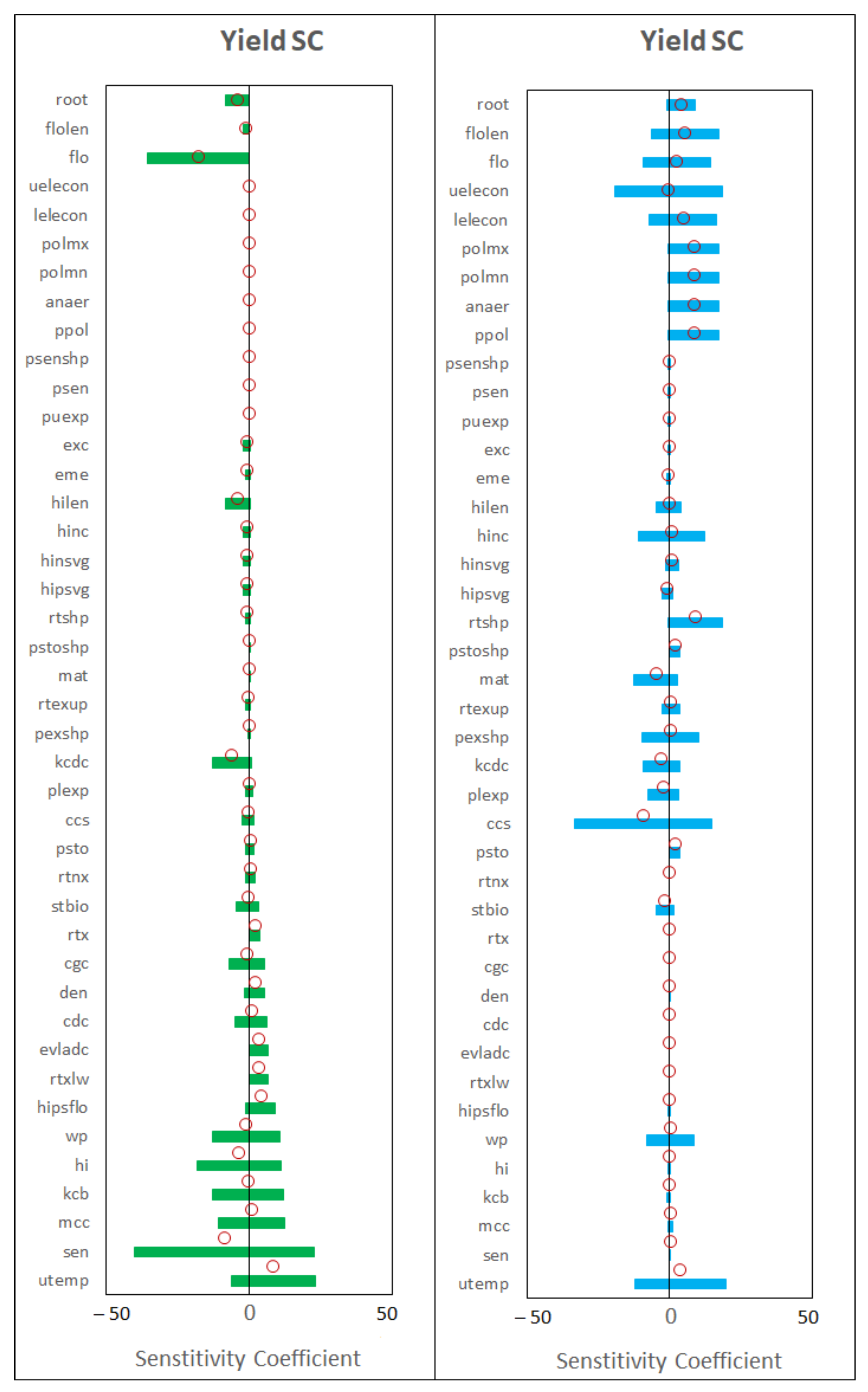
Figure 3 shows the sensitivity coefficients (SC), which indicate relative changes in a crop’s yield (Y-SC) or evapotranspiration (ET-SC) in response to a ±1% change in each of the 42 crop parameters defined in the crop-file of the Aqua-Crop model. The average Y-SC and ET-SC varied in the range of (−17.8–+8.3)% and (−9.1–+9.1%), respectively. The crop’s yield was the most sensitive to “flo” (i.e., GDD from sowing to flowering), “Psen” (i.e., Upper threshold of soil water depletion factor for canopy senescence), and “utemp” (i.e., Upper temperature above which crop development no longer increases with an increase in temperature). A ±1% change in these parameters caused an average change of −17.7%, −8.6%, and +8.6% change in crop’s yield. ET-SC, however, had the largest value (i.e., in absolute term) for “Kcb” (i.e., Crop coefficient when canopy is complete but prior to senescence), “evladc” (i.e., Effect of canopy cover in reducing soil evaporation in late season), and “hipsflo” (i.e., possible increase of HI due to water stress before flowering). Relevant ET-SC shows that a ±1% change in these parameters caused an average change of −9.1%, 9.1%, and 8.7% in ET, respectively. The significant effects of these parameters on the crop’s yield and/or ET has been reported by earlier researchers as well (e.g., [22,28,52,55]). It is worth mentioning that either Y-SC or ET-SC were affected by the crop type and geographic location, which resulted in a range of estimated values for these coefficients. Such variability is also supported by other researchers (e.g., [38,39]). Hence, we calibrated the model per crop per county and selected the most sensitive parameters accordingly.

3.1.2. Calibration and Validation

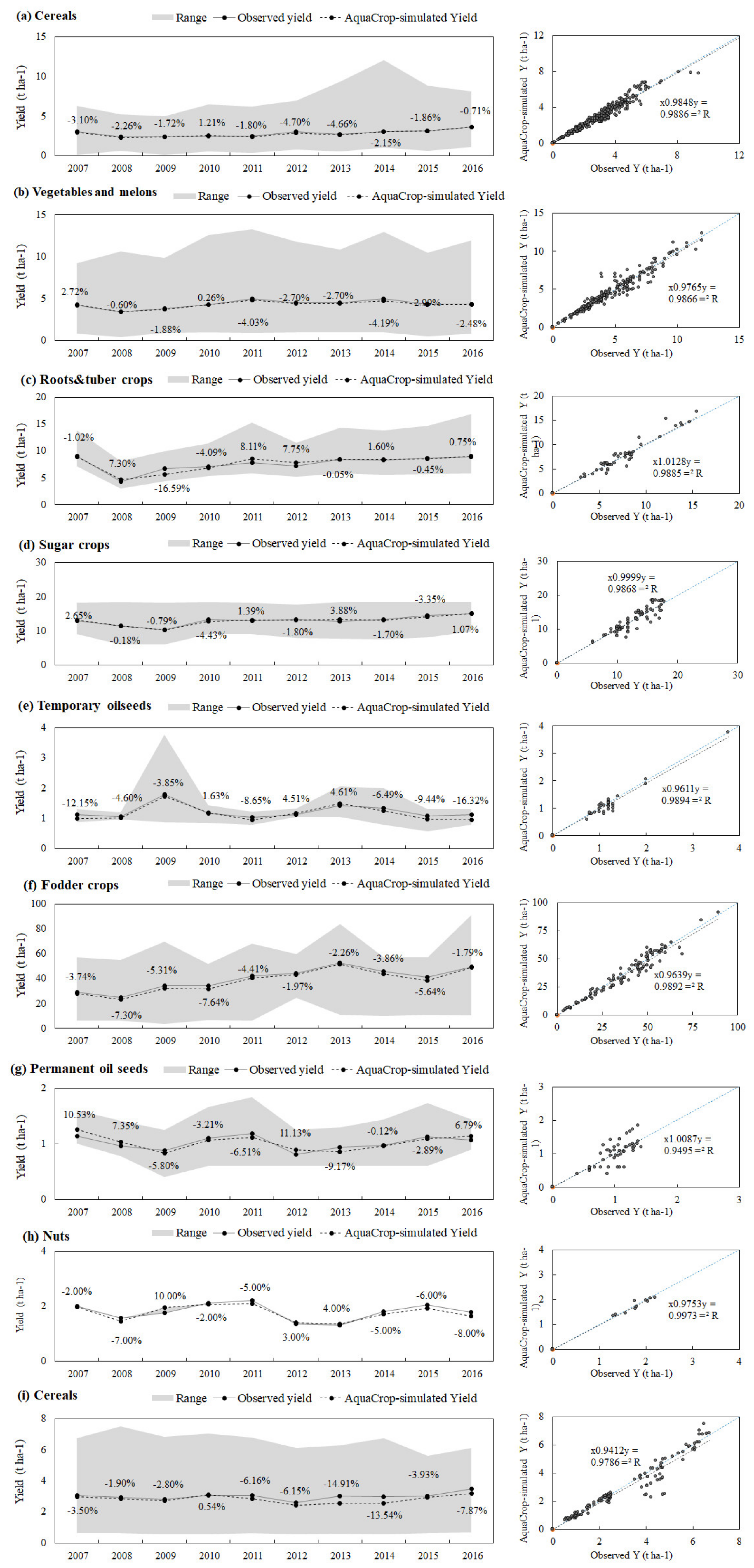
Figure 4 compares observed and model-simulated crop yields (Y) per crop category (i.e., averaged over the entire province) for the calibration period, which indicates the capability of the AquaCrop model in capturing temporal and spatial trends of Y. Generally, simulated Y agreed well with the observed one with a R² ranging from 0.97 to 0.99. The close match between the observed and the AquaCrop-simulated Y was also observed in other studies for different crops [23,38,40]. We also quantified the agreements between observed and AquaCrop-simulated yields during the calibration and validation periods using nRMSE, nMBE, and NS-EF (

Table 5. Average of evaluation criteria including normalized root mean square error (nRMSE), normalized mean bias error (nMBE), and Nash-Sutcliff efficiency coefficient (NS-EF) during the calibration (2006–2016) and validation (1986–2005) periods.

Period	Parameter	Staple Crops	Cash Crops	All Croos
Calibration	nRMSE (%)	(0.35)–(11.7)	(0.73)–(7.93)	(0.36)–(8.96)
	nMBE	(−0.61)–(3.45)	(−1.75)–(1.88)	(−0.83)–(1.97)
	NS-EF	(0.87)–(1)	(0.51)–(1)	(0.73)–(1)
Validation	nRMSE	(0.33)–(10.8)	(0.76)–(9.9)	(0.37)–(9.1)
	nMBE	(−0.64)–(5.51)	(−1.82)–(2.96)	(−1.25)–(2.23)
	NS-EF	(0.75)–(0.99)	(0.52)–(0.99)	(0.68)–(0.98)

) in addition to visual inspections. The average values of nRMSE, nMBE, and NS-EF varied in the ranges of 0.36–8.96%, (−0.83)−1.97%, and 0.73–1 during the calibration period, and in the ranges of 0.37–9.1%, (−1.25)−2.23%, and 0.68–0.98 during the validation period. These results indicate that the AquaCrop model can be successfully used for WF accounting in the study area.

3.2. Food Availability

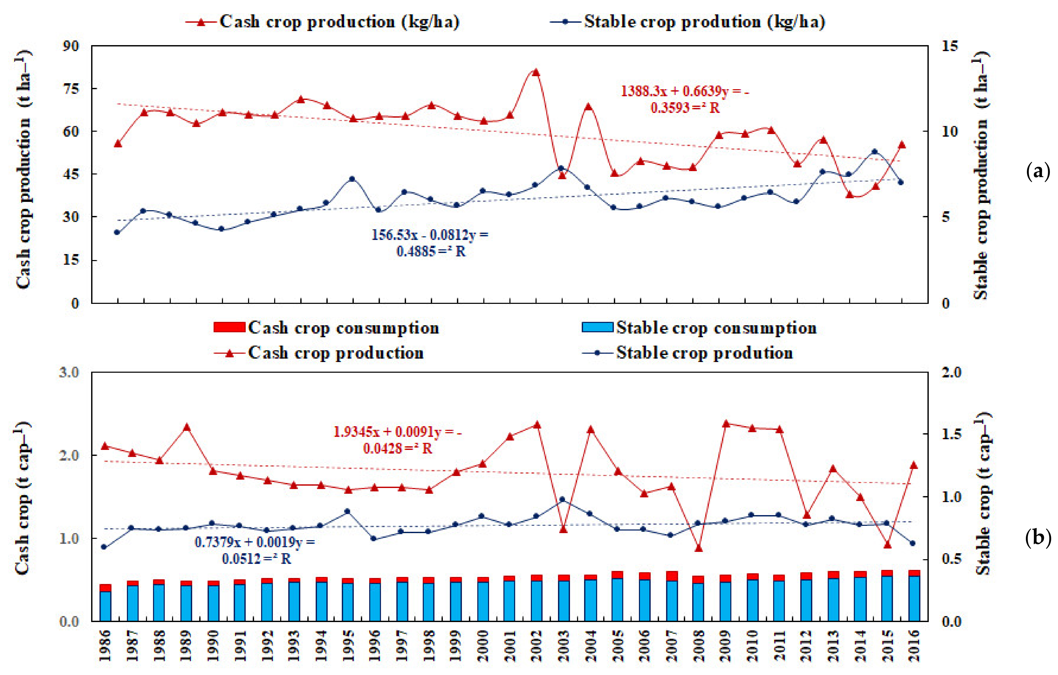
Figure 5 shows the temporal growth in staple and cash crop production, expressed as t ha⁻¹ and kg cap⁻¹, over the study period (1986–2016). The staple crop’s yield (kg ha⁻¹) increased by 72%, from 4.1 t ha⁻¹ in 1986 to 7.0 t ha⁻¹ in 2016. Such an increase was mainly attributed to the excessive use of agrochemicals [25] and converting rainfed lands to irrigated ones over the study period, which resulted in an 84% increase in total staple crop production (t y⁻¹) despite a slight increase of 8% in their harvested area. Nevertheless, the positive impact of yield improvement was overridden by a 77% increase in population and a 50% increase in their per capita staple crop consumption during 1986–2016. Hence, only a 5% increase occurred in staple crop availability, from 591 kg cap⁻¹ y⁻¹ in 1986 to 620 kg cap⁻¹ y⁻¹ in 2016.

Cash crop’s yields, however, followed slightly a decreasing trend with an average annual reduction slope of 0.66 t ha⁻¹ y⁻¹ over the period of 1986–2016. Such a reduction corresponded with a 57% and 60% increase in cash crops’ total production and harvested area in the same period. Consequently, cash crop availability decreased by 12%, from 2100 kg cap⁻¹ in 1986 to 1890 kg ha⁻¹ in 2016 despite an 18% increase in cash crop demand in this period.

3.3. Water Footprint Profile of Khuzestan Province

3.3.1. Consumptive Water Footprint

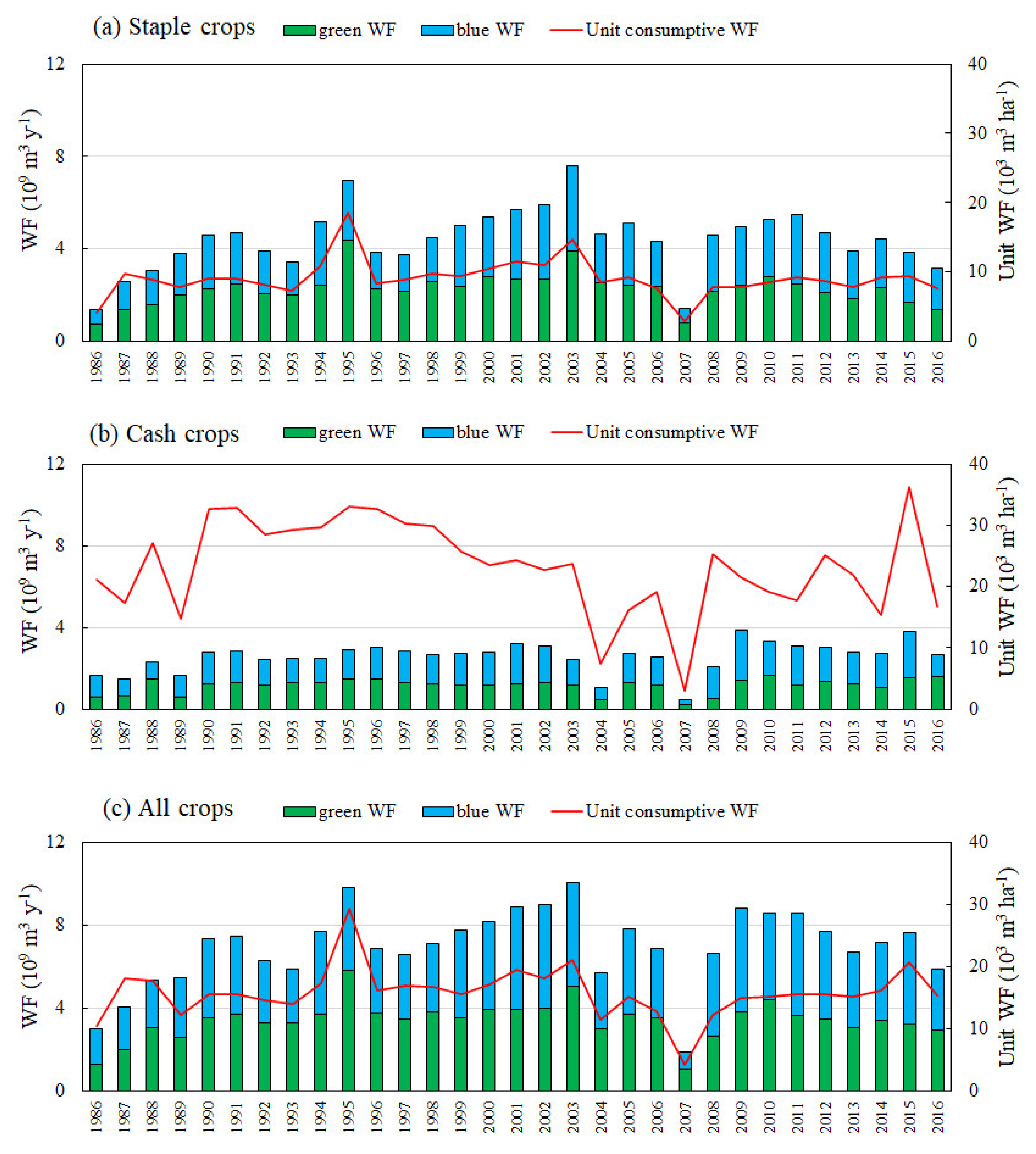
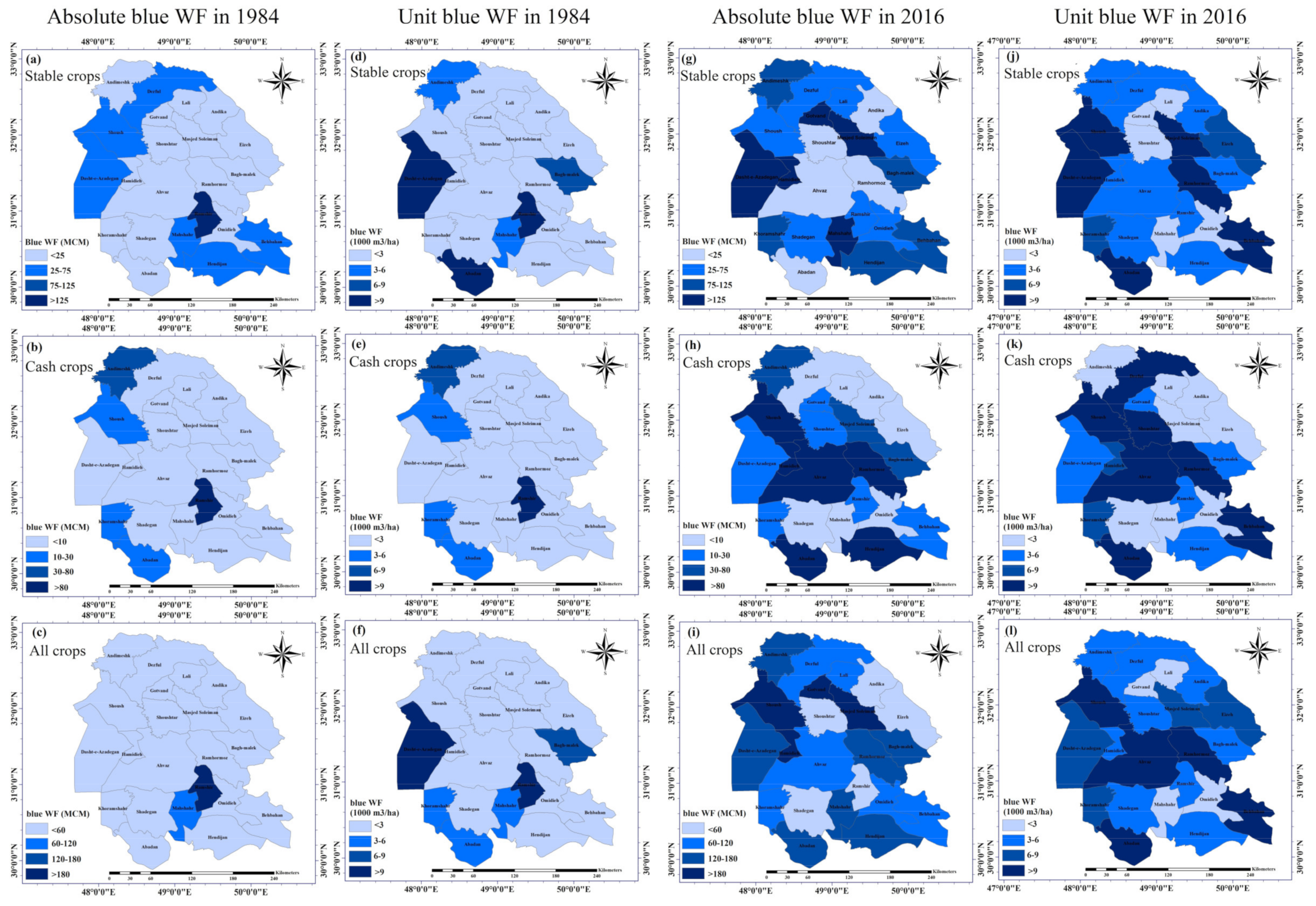
Compared to 1986, and along with a 63% increase in all crop production (staple plus cash crops), the total blue WF increased by 80%, from 1.82 billion m³ y⁻¹ in 1986 to 3.27 billion m³ y⁻¹ in 2016. The unit blue WF also increased by 53%, from 3700 m³ ha⁻¹ in 1986, to 5660 m³ ha⁻¹ in 2016. The increasing blue WF trend was observed for either staple or cash crops in the study area. The average annual increase in the unit blue WF of these crop categories was 810 m³ ha⁻¹ y⁻¹ and 302 m³ ha⁻¹ y⁻¹, respectively. The increased blue WF mainly occurred at the cost of overexploiting groundwater resources. In 1986, a total of 125 million m³ of groundwater resources were used in agriculture, which contributed 11% in total blue water consumption in this sector. Such consumption increased to 1161 million m³ in 2016, which contributes 33% to the total agricultural blue water consumption. The considerable reduction in the blue WF in 2007–2008 growing season was due to a severe drought that occurred in this period.

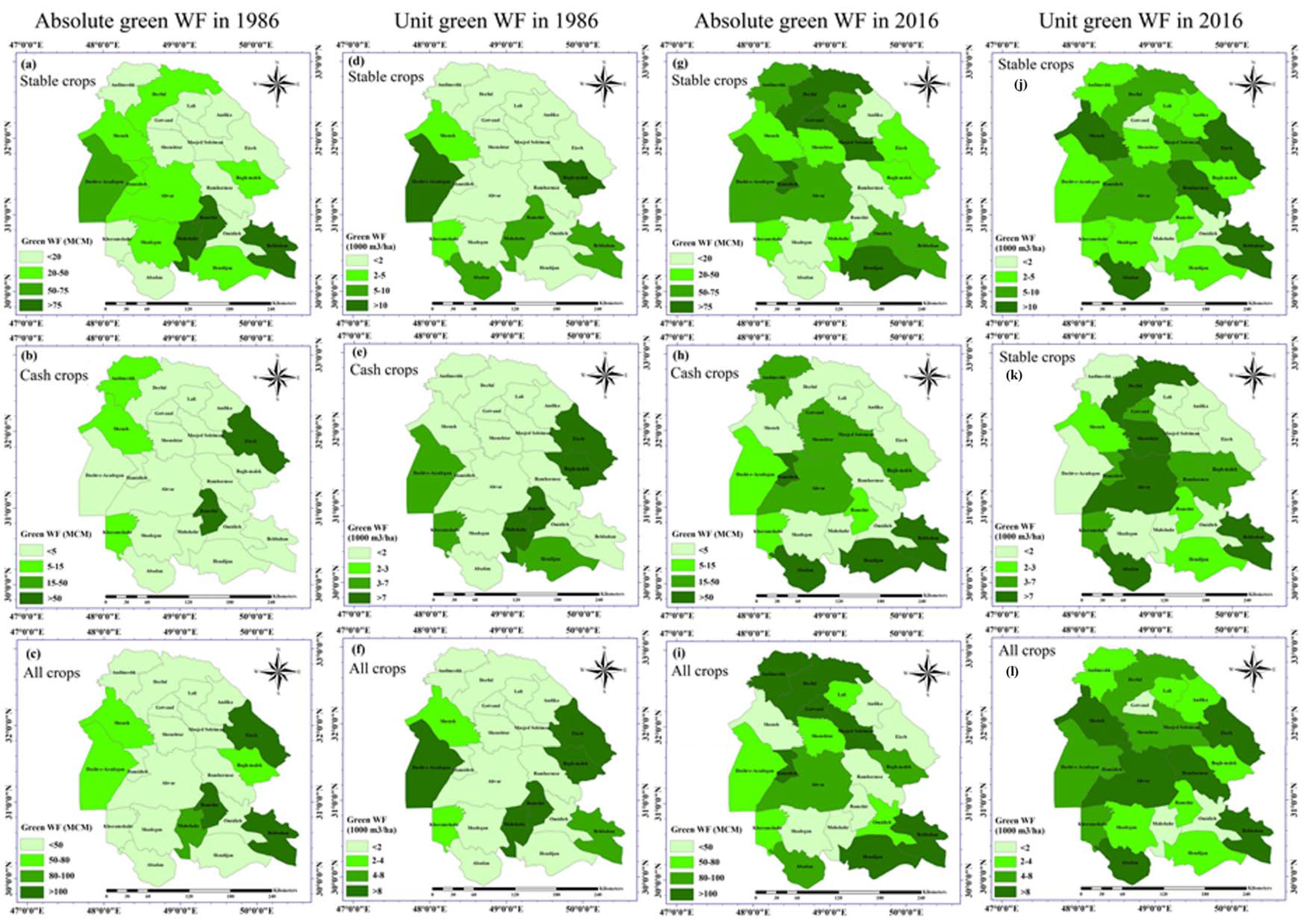
Figure 6 shows that despite a slight increase of 12% in the total green WF related to crop production in the study area (i.e., from 2.78 billion m³ y⁻¹ in 1986 to 3.14 billion m³ y⁻¹ in 2016), the green water contribution to the consumptive water footprint decreased from 60% in 1986 to 48% in 2016. In addition, the green crop water use (m³ ha⁻¹) followed a decreasing pattern with an average annual reduction of 180 m³ ha⁻¹ y⁻¹.

Figure 7 and Figure 8 show the spatial distribution of blue and green crop water use (m³ ha⁻¹) and WFs (total m³) in 1986 and 2016. In 1986, different counties consumed 2–485 million m³ y⁻¹ of blue water in the crop production process, roughly 52% of which was consumed in Ramshir county. In 2016, the blue water consumption at the county level increased to 20–572 million m³ y⁻¹, and different counties had a contribution of 0.6–18% in this total. Roughly 60% of the counties (13 county) experienced a blue crop water use increase, and the other 9 counties experienced a reduction. Moreover, green water consumption for crop production in different counties increased from 1.47–381 in 1986 to 7.8–1305 in 2016. In two-thirds of the counties (i.e., 15 out of 22 counties), green crop water use increased in 2016.

3.3.2. Degradative Grey Water Footprint

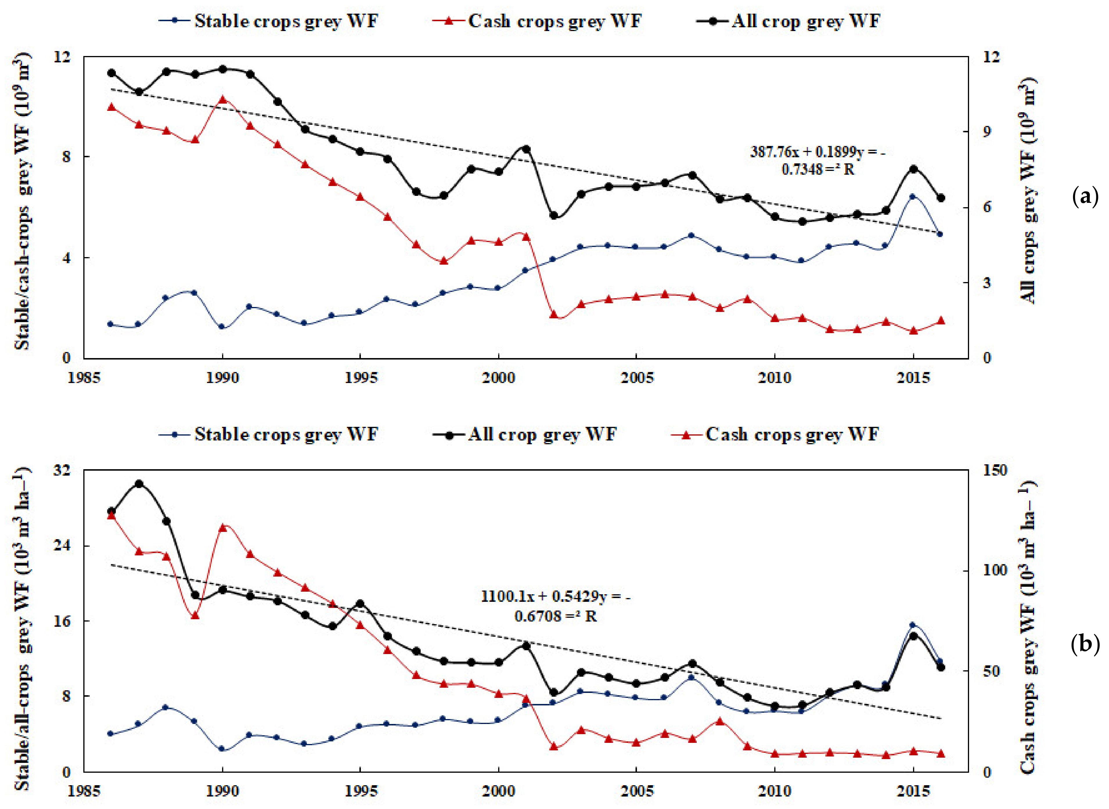
In contrast to the consumptive WF, the grey WFs related to all crop production in terms of m³ ha⁻¹ and total (m³ y⁻¹), followed by a decreasing trend with average annual reduction rates of 140 m³ ha⁻¹ y⁻¹ and 0.17 billion m³ y⁻¹, respectively (Figure 9). Such reduction mainly occurred within cash croplands. The total grey WF related to cash crops production decreased by 99%, from 9.7 billion m³ in 1986 to 0.1 billion m³ in 2016; such reduction occurred with an annual average reduction of 3940 m³ ha⁻¹ y⁻¹ in grey WF in cash croplands. Nevertheless, the grey WF related to staple crop production increased by 293%, from 1.6 billion m³ in 1986 to 6.3 billion m³ in 2016, along with an annual average increase of 260 m³ ha⁻¹ y⁻¹ in grey WF.

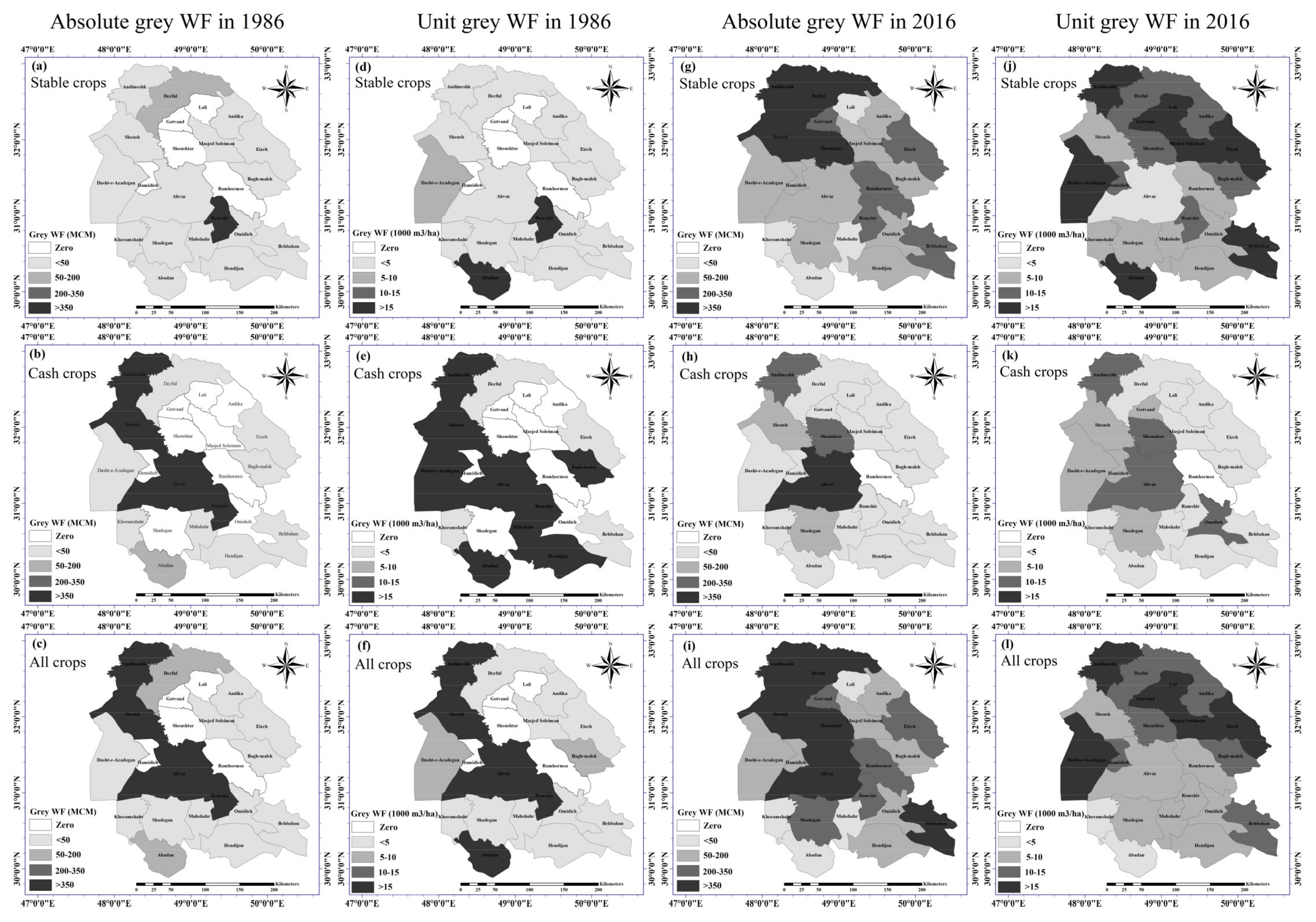
Depending on the available cropping pattern, different counties had a different grey WF (m³ ha⁻¹), and different contributions in the total grey WF (m³ y⁻¹) related to crop production in the study area. In 1986, about 85% of the total grey WF originated from the three counties of Ahvaz (29%), Andimeshk (28%), and Ramshir (28%), and the other 19 counties had a total contribution of 15% in the total grey WF (Figure 10). In 2016, Andimeshk stood as the main grey WF producer, with a large contribution of 40% in total. Nevertheless, the grey WF per hectare in different counties was reduced by 61–99% in different counties in this year. The only exceptions were Masjed-Soleiman and Lali counties, in which the grey WF per hectare increased by 266% and 95%, respectively. Such an increase was mainly due to a considerable increase in staple crop production in 2016.

3.4. Sustainability Assessment of Water Use

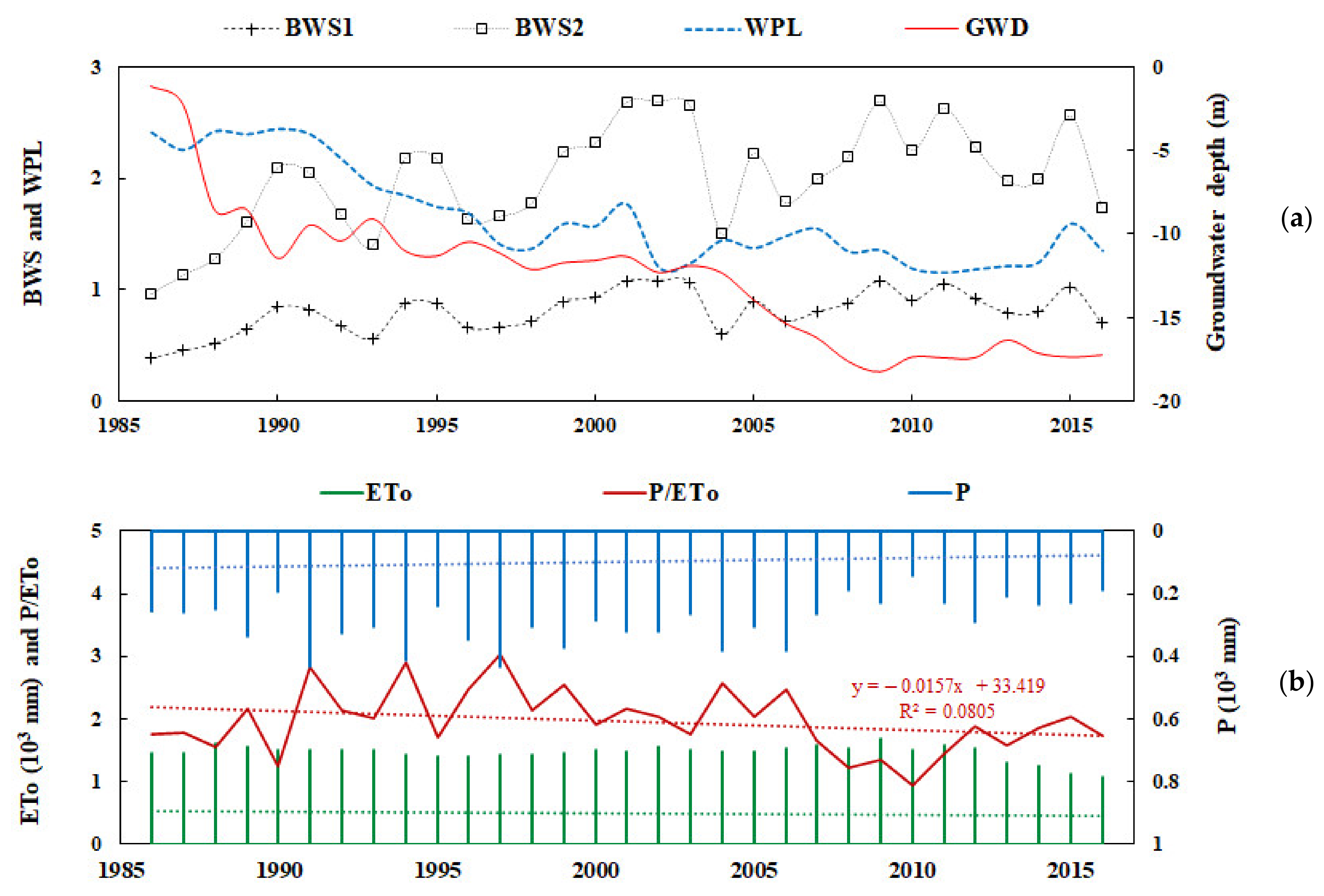
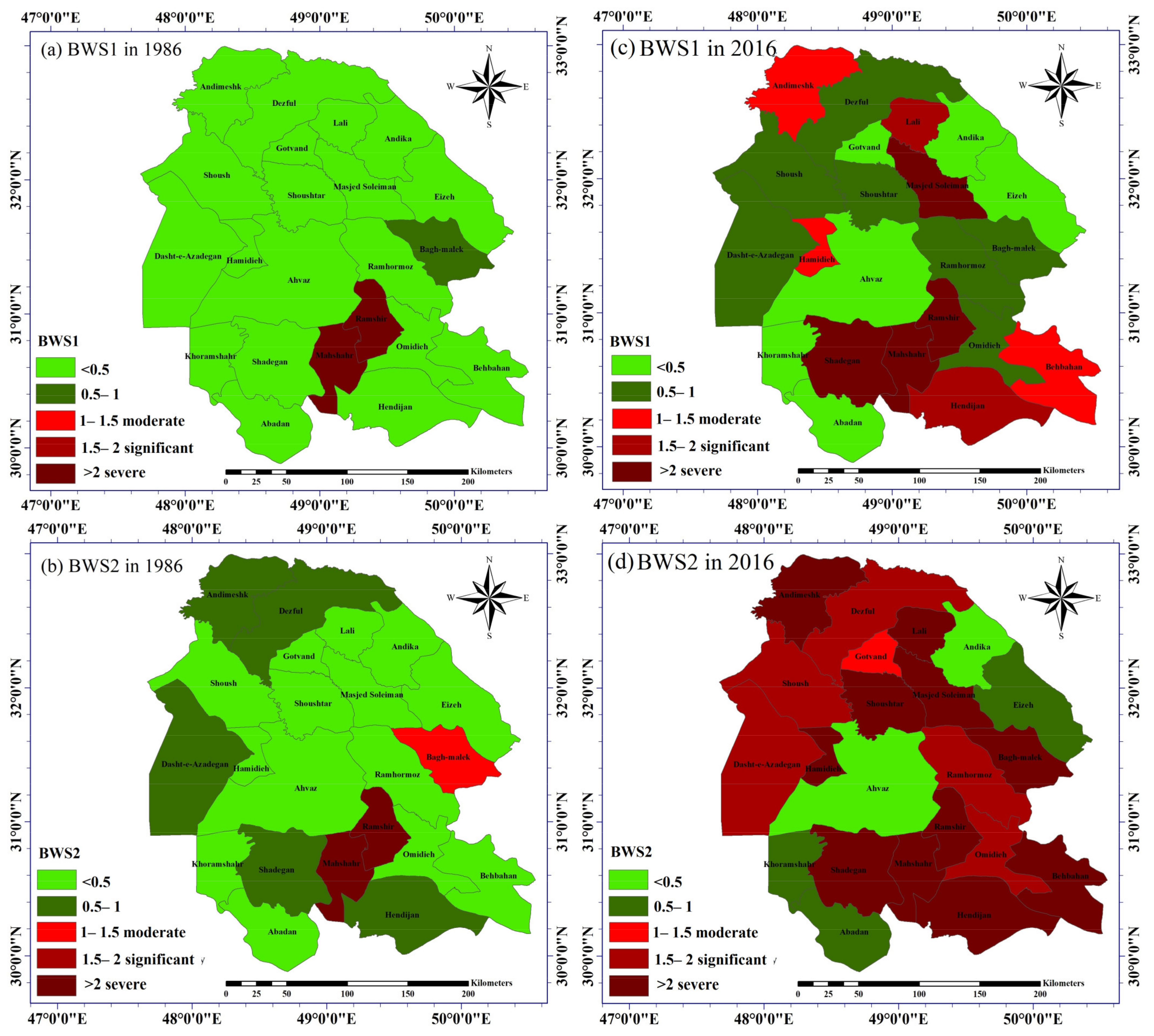
Figure 11 shows the temporal growth of water scarcity indices (BWS1, BWS2, and GWD) and water pollutions status (WPL) over the period of 1986–2016. Crop production raised the BWS with an average annual increase of 5% over the period of 1986–2016. In six years, the BWS exceeded 1, which indicates that blue water consumption at the cost of violating environmental flow requirements (EFR) in these hotspot years. Spatial hotspots also increased in the study area. The number of counties with a BWS1 > 1 increased from one county in 1986 to nine counties in 2016, and the number of counties with a BWS2 > 1 increased from two counties in 1986 to 18 counties in 2016 (Figure 12).

Blue water overexploitation also caused the groundwater level to deplete from 1.2 m in 1986 to 17.3 m in 2016. Climate change had less contribution in blue water overexploitation rather than the other factors since P/ETo had a slight increase of 1.1% over the study period. Despite the growing BWS, the WPL followed a decreasing trend, as it was reduced by 44%, from 0.48 in 1986 to 0.27 in 2016. Neither in 1986 nor in 2016 did the WPL exceed one, which indicates that local water bodies have enough capacity to assimilate the pollutant loads (Figure 12).

3.5. Synergies/Tradeoffs between SDG Indicators

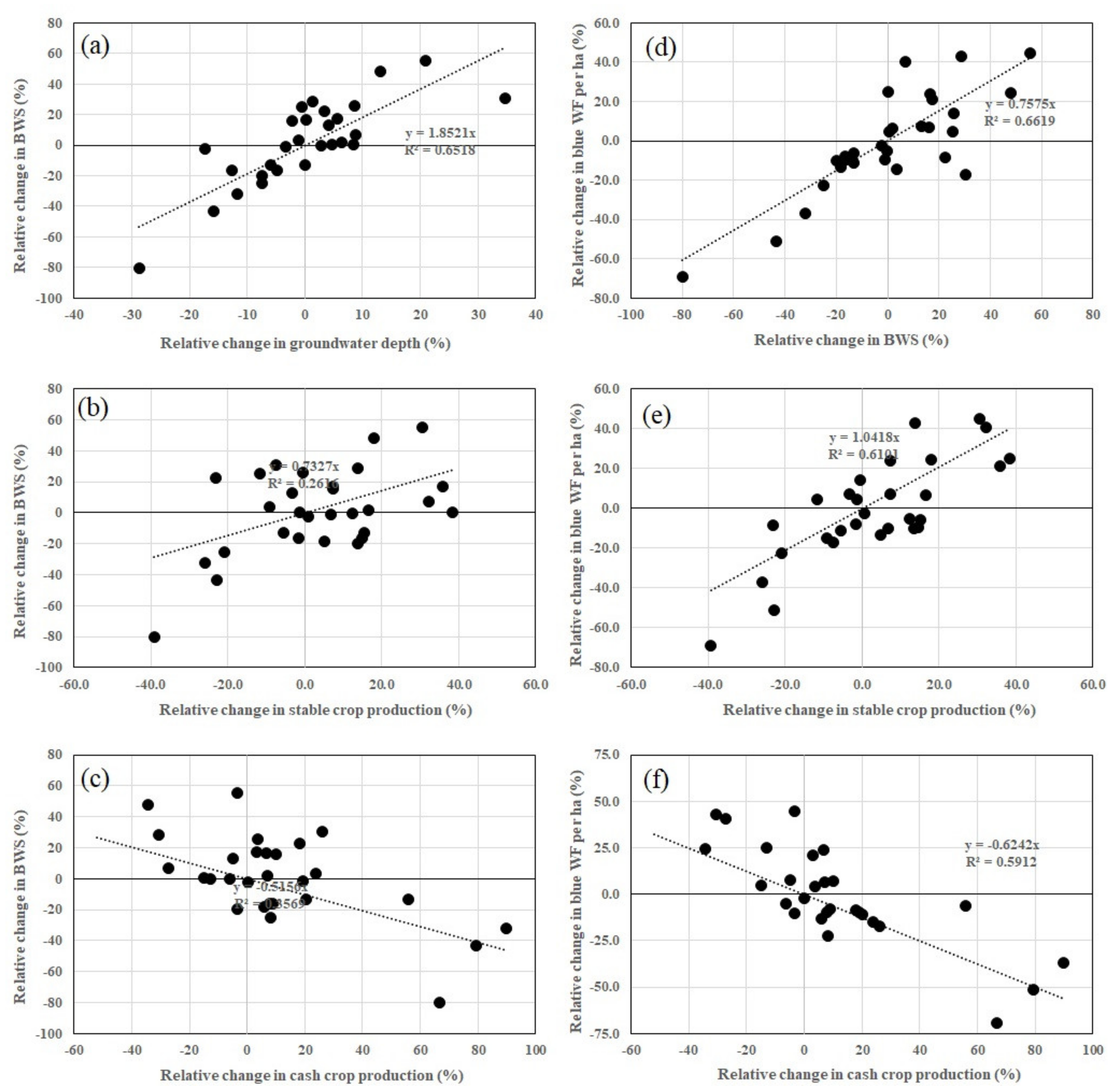
Scatter plots between the BWS and food production indices show that a unit increase in staple crop production (1%) was at the cost of a 1.1% increase in blue crop water use (m³ ha⁻¹), which consequently resulted in a 0.7% increase in BWS (Figure 13). In contrast, a crop water use increase in cash crop production corresponded with a 0.6% decrease in unit blue water consumption, which, consequently, caused a 0.5% alleviation in the BWS in the study area. When assessing scatter plots between the crop production and BWS (i.e., without disaggregating crops into staple and cash crops), the BWS decreased by 1.2% along with a unit increase in total crop production. Such a result is due to the larger contribution of the cash crop productions in total. Figure 13, however, shows the negative impact of groundwater overexploitation on BWS enhancement; a unit increase in GWD raised the BWS by 1.9% in the study area.

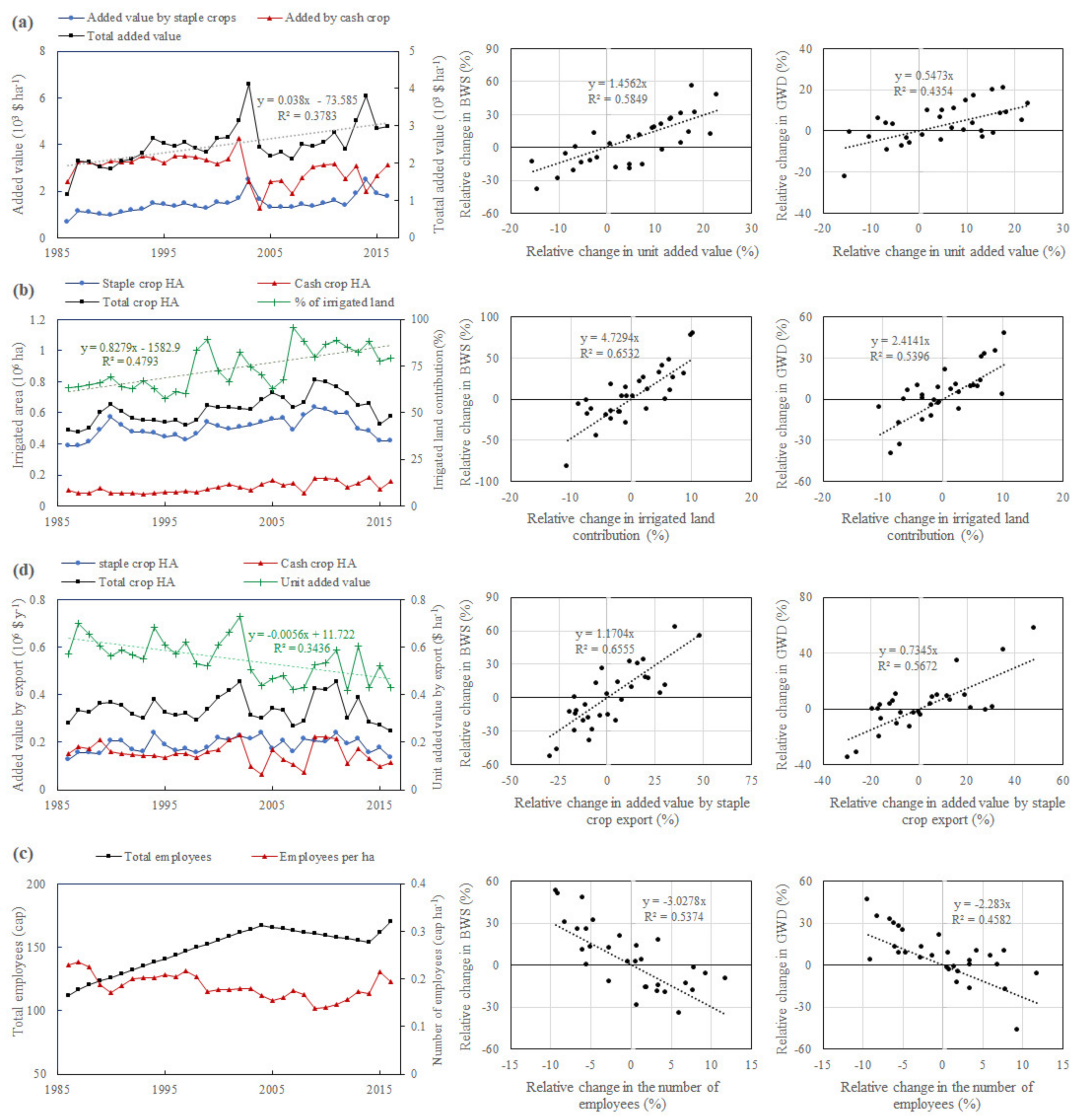
Raising the BWS corresponded with some socioeconomic benefits in the study area (Figure 14). The irrigated, harvested area increased by 18% at the cost of an 80% increase in BWS, which consequently caused a 198% increase in the added-value from crop production, a 5% increase in the added-value from the staple crop export, and a 51% increase in the number of employees in the agricultural sector. Such an assessment per unit harvested area also demonstrates that prospering residents’ socioeconomic status occurred at the cost of environmental deterioration. Compared to 1986, the unit added-value from crop production (crop’s economic productivity, $ ha⁻¹), unit staple crop export ($ ha⁻¹), and the number of employees per unit harvested area (cap ha⁻¹) increased by 154%, 28%, and 29%, respectively, in 2016. Along with such improvement, BWS1 increased from 0.39 in 1986 to 0.70 in 2016, BWS2 increased from 0.97 in 1986 to 1.74 in 2016, and GWD increased from −1.19 m in 1986 to −17.50 m in 2016.

4. Discussion

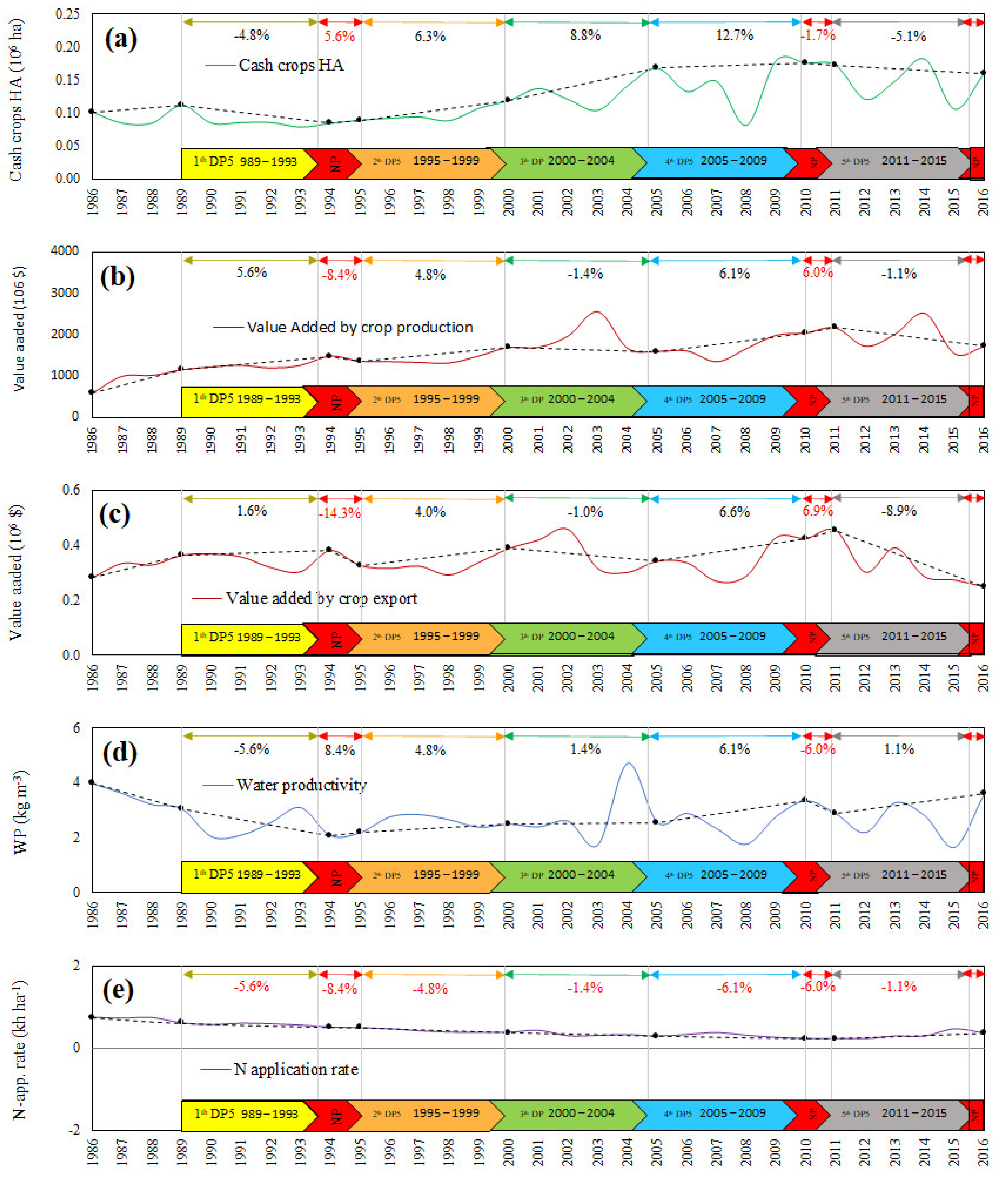
Along with a comprehensive water footprint assessment, we analysed the sustainability and efficiency of water use in food production in the agricultural backbone of Iran over the period of 1986–2016. Our results indicate a steady growth of blue water scarcity and groundwater depth depletion along with a rising contribution of an inefficient water footprint in total. In contrast, the region benefited from a 54% increase in total crop production (staple plus cash crops) over this 30-year period. Such results show trade-offs between food security (SDG2) and water efficiency/scarcity (SDG6) in the study area. Indeed, questing for food self-sufficiency imposed remarkable costs to the environment. Supplying food demand with unsustainable use of Iran’s water resources has been confirmed by other researchers as well [41,42,43]. Hence, we made an institutional assessment in order to investigate the impact of governmental policies and targets on the unsustainable agricultural growth in terms of water use. The influence of these policies was quantified in terms of changes in irrigated harvested area, value added from crop production and export, N application rate, and water productivity (Figure 15). In the following subsections, the status of the current agroecosystems is discussed in the context of these DV₅ to analyse how political attitudes drove water-related environmental challenges in the study area.

4.1. Evolution of Irrigated Harvested Area

Along with the raising thirst for development after the revolution in 1979, the policy of self-sufficiency in food production was implemented in the first DV₅ in 1989 and has been considered since after. Three major indicators were considered by the government to evaluate the achievements, including evolution of (i) irrigated harvested area, (ii) value-added from crop production, (iii) and value-added from crop export. The government supported the expansion of the irrigated harvested area by implementing some facilitating tools like constructing small and large dams, expanding irrigation and drainage networks in a large area, subsidizing agricultural water consumption, and developing local water markets (Table 3). Such interventions resulted in a 41% increase in the irrigated harvested area in Khuzestan province over the period 1986–2016 (Figure 2). From 1989–1993 (first DV5), the country was in the Iran–Iraq war and, therefore, this expansion mainly occurred within the staple croplands. After, boosting cash crop production was considered, which resulted in a steady growth in these crops’ harvested area over the period of 1994–2009 (Second to fourth DV5s). Such an increase was mainly encouraged by passing the legislation for constructing seven sugarcane agro-industries in an area of 84 thousand ha in Khuzestan province in 1989. Along with that policy, the sugarcane harvested area increased by 240%, from 26.4 thousand ha in 1990 to 89.6 thousand ha in 2016 (Figure 15). Nevertheless, the cash crop harvested area was reduced by 5.1% over the period of 2011–2015 (fifth DV5), although it was supposed to grow by 3% in this period. Such a reduction mainly occurred within sugar-crops and, temporarily, oilseeds croplands. On the other hand, irrigated fodder croplands and orchards were significantly expanded during the fifth DV5 period. While achieving self-sufficiency in crop production was a concern in the first to fourth DV5, the government planned to achieve self-sufficiency in livestock production as well in the fifth DV5. Such a policy caused a 22% increase in the irrigated harvested area of fodder crops. The steady growth of fruits contribution, and particularly nuts, in the total irrigated harvested area also corresponded with the government’s plan for developing orchards in the steep lands of Khuzestan province. In 2009, a total of $293 thousand was allocated to implement such expansions in 23 counties of Khuzestan province during the fifth DV5 period.

4.2. Agricultural Economic Growth

The agricultural sector was set as the main core of economic development since the second DV₅. Accordingly, relevant policies and targets, like supplying required inputs and machineries, developing manufacturing industries, compensating farmers for 50% of production losses, issuing land ownership documents, and providing economic support for increasing crop production, were implemented in order to gradually move toward an agricultural-based economic development (Table 2). Such encouragement resulted in a 199% increase in the value-added from crop production in the study area, from $574.7 million in 1986 to $1717.6 million in 2016. The annual growth in the agricultural value-added was slightly less than the organized one in the first DV5 (i.e., 6.1% versus 5.6%). A negative growth was observed from 2000–2004 (i.e., the third DV5) with an average annual rate of −1.4%. Yield reduction was affected by a severe drought event, which occurred over the period of 1999–2002, was the cause of the decreasing trend of agricultural economic growth during this period (2000–2004). In the fifth DV5, such value was −1.1%, although the government planned to have an annual growth of 7% over the period of 2011–2015. Not only did it not meet the expected agricultural value-added growth, but also it did not achieve the other planned programs during the fifth DV5 period; this was mainly due to restricted international resource mobilization, which roots into the tightened sanctions placed by the USA over the period of 2012–2015 (i.e., before reaching a nuclear deal in 2015). Practical complexities, which were induced by sanctions, affected Iran’s economic growth and environmental status in terms of the following points [41]. (i) Iran’s access to technology, services, and know-how was restricted in official channels, and its ability to unofficially purchase them in the international markets also decreased due to a considerable increase in the relevant costs. Such challenges consequently resulted in a highlighted reduction in the efficiency of water and agricultural sectors. (ii) The opportunity of receiving international aid for the surviving environment was lost in this period (i.e., the World Bank fully stopped their support; only 15% of $4.2 million of the allocated fundings from the GEF (Global Environmental Facilities) was utilized during 2010–2014; Quercus ceased its support for constructing a 500-million euro solar power plant which was supposed to have a total capacity of 600 MW; and etc.). (iii) Obstacles for money transfer restricted international trades and reduced the number of Iran’s trading partners (i.e., this point raised serious challenges for importing the required inputs for improving crop production or exporting agricultural products to the other countries, particularly those which were directly impacted by the USA. Acquiring goods that were exempted from economic sanctions was also restricted in this period due to the long process for getting the required licences). (iv) A lot of intergovernmental agencies/organizations who were supposed to collaborate with developing plans in the agricultural sector closed their offices in Iran and stopped their supports (i.e., they justified their decision with obstacles that they faced in transferring funds through the official banking system and stopped their collaborations without paying any penalties to the country). Part of these supports, for instance, were to reduce poverty; enhance food, water, and nutritional security; improve environmental health, and increase the resilience of current agroecosystems to the featured global challenges like climate change.

Poor economic status during the sanctions caused the country to adopt a low-productive production system to survive. However, other reasons also caused a gap between what was planned in the fifth DV5 and what was achieved in reality; the most important challenges are an imbalance between the planned targets and the ecological potential of the country, low efficiency and productivity of the resources and inputs due to poor management, and low technical capacity due to the lack of required infrastructures. The latter was particularly the case for the first to third DV5s.

4.3. Trade Policies

Since 1986, the government has tried to increase the contribution of export-oriented crops in total international export by implementing encouraging policies and targets like tax exemption for agricultural product export, supporting internal products through setting proper tax for similar external products, setting a target for annual increase in the contribution of none-oil products export including agricultural commodities, and giving special attention to the export of oil-crops, horticultural crops, and olives. Such an increase occurred over the period of 1989–1999 (first and second DV5) and 2005–2009 (fourth DV5), although it had less annual average growth compared to the planned one (4% versus 8.4% in the second DV5, and 6.6% versus 10% in the fourth DV5) (Figure 15). Over the period of 2000–2004 (third DV5), value added from crop export decreased by 1%, which was mainly attributed to the impacts of the severe drought that happened over the period of 1999–2002. A reduction in the crop-export-related value-added was the largest over the period of 2011–2015 (−8.9%). As explained before, Iran lost its opportunity to contribute to the international markets due to money transfer obstacles and the reduced number of trading partners under tightened sanctions in this period. On the other hand, the country mainly focused on staple crop production in this period rather than cash crops in order to address its concerns about food security, which was threatened by the reduced food imports under sanction status.

4.4. Fertilizer Application

The decreasing trend of N-application in croplands over the period 1986–2011 (Figure 15), along with the reduced WPL in this period (Figure 11) indicates that the country performed better regarding pollution controls. Some policies like substituting chemical fertilizers with biological ones, enforcing the production units to reduce their pollution loads to the environment, and determining allowable rates of fertilization encouraged the reduction of diffuse pollution from the croplands to the environment. Nevertheless, both the N-application rate (1.1%; Figure 15) and the WPL (34%; Figure 11) increased over the period of 2011–2015 (i.e., the fifth DV5). Under the enforced sanctions, the government decided to defeat its economic recession through unsustainable development. Hence, boosting the application of chemical fertilization within croplands was considered as one of the solutions to defeat income and production deficits (Figure 15). While such a strategy periodically reduced the negative impacts of the sanctions on Iran’s economy, it created a deteriorating-economy which can result in long-term impacts on the environment. Pollution loads beyond the assimilation capacity of the environment, and the consequent increase in the WPL is only one of these cases. Karandish [25] also demonstrated that the WPL is beyond 1 in more than half of the county due to excessive chemical fertilizer application within croplands, indicating that the assimilation capacity in these regions is exceeded. On the other hand, the lack of access to technologies with environmental standards caused Iran to produce its fertilizers through unsustainable processes or to import low-quality fertilizers from a restricted number of its trading partners [44]. Such activism undoubtedly leads to increased emissions [41]. For instance, the fear of retaliation caused Siemens not to ship the syngas compressors which were required for the Zanjan Fertilizer Project, and, therefore, Iran purchased similar products produced by China with lower environmental standards, resulting in more emissions through the fertilizer production process [44]. This story indicates that the rate of emissions should be considered in addition to the WPL when assessing the real environmental impacts of fertilizations. Nevertheless, such estimations were out of the scope of this paper.

4.5. Water Productivity

Improving water productivity was considered since the beginning of the second DV5 in 1995. Since then, the WP increased by 4.8%, 1.4%, and 6.1% over the period of the second DV5 (1995–1999), third DV5 (2000–2004), and fourth DV5 (2005–2009). The gap between the achieved and expected WP was due to less attention to some policies like participatory water management, prevention of land fragmentation, and the prevention of the cultivation of water-intensive crops like rice, although it was implemented in all DV5s as well as the lack of executive laws to ensure the implementation of policies in practice. Our water scarcity assessment also denotes that the WP improvement in this period did not help to reduce pressure on blue water resources (Figure 11). Indeed, the benefits from the WP improvement was offset by using saved water for expanding irrigated croplands in the study area (the rebound effect or Jevons paradox).

The negative trend of the WP growth over the fifth DV5 was attributed to the recession economy that occurred under the enforcement of sanctions in this period. Over the period of 2011–2015, the WP decreased by 1.1%, although it was supposed to increase by an annual average rate of 1% in the fifth DV5. The government planned to strengthen its control over water consumption through enriching volumetric water delivery systems, developing modern and efficient irrigation and drainage networks, developing water-productive production systems, and setting caps on surface and groundwater withdrawal (Table 3). Nevertheless, it failed in achieving its targets in the fifth DV5 under the pressure of tightened sanctions over the period of 2011–2015. Hence, the natural-resource intensity increased in Iran, and economic development occurred at the cost of environmental degradation. There is some evidence that shows that the persisting value-added from the agricultural sector in this period occurred at the cost of unsustainably depleting water resources. For instance, the groundwater budget deficit was supposed to be alleviated by 25%; however, groundwater consumption increased from 988 million m³ in 2011 to 1161 million m³ in 2015. This result agrees with earlier findings, which indicated the exploitation of non-renewable groundwater resources for human appropriation (groundwater mining) in Iran [45,46,47,48]. In addition, irrigation efficiency was supposed to increase by 40% in order to reduce the pressure on the limited blue water resources; however, the BWS increased by 1.2% along with a 14% increase in blue water consumption. The reduced flow of the main rivers in Khuzestan province and the significant reduction in the level of groundwater resources is proof to this claim [41,49,50].

The positive correlation between the agricultural value-added and blue water consumption in the agricultural backbone of Iran (Figure 13 and Figure 14) indicates that the country’s economy is extremely dependent on depleting water resources and, therefore, cannot be sustainable in the long term. According to SDG 6, decoupling economic growth from the use of natural resources is essential for achieving a sustainable development (FAO and UNW, 2021). Indeed, water scarcity should not be a constraint for economic and social growth. However, the prioritization of achieving SDGs depends on the income level of a country [51]. When a financial crisis becomes a threat to the composition of the national economy, the environmental sustainability has to compete with other issues like food security, employment, national security, etc. [52]. Under such circumstances, the environment is sacrificed in order to address the other priorities. The lower the income level of a country, the lower the importance of environmental issues and the less progress on implementing SDGs [42,53]. Indeed, it is economically costly for a sanctioned country to prioritize its environment. Hence, it continues its thirst for development with an intensive use of natural resources and, in many cases, like Iran, can cause irreversible environmental degradation.

The international virtual water trade was introduced as an effective pathway for reducing such a dependency [54]. Water-intensive and/or economically low-productive crops are supposed to be imported from the other countries where the same crop is produced with higher water productivity and with a higher contribution of the green water in the total water consumption [55]. Nevertheless, involving such trades is restricted under sanction status due to the restricted number of trading partners on the one hand (i.e., only countries which do not get direct benefits from the US would dare contribute in such a trade) and money transfer challenges on the other hand.

Another issue which is loosened in a sanctioned country is its unlikely ratification of international environmental cooperation and activisms. Under limited access to the international markets, pursuing unsustainable agricultural policies and activisms in order to fulfil food demands and to reduce dependency on foreign countries will not let Iran be committed to international environmental agreements. Hence, the negative impacts of sanctions will not be limited to Iran and indirectly creates struggles for the other countries in the world through raising global warming.

5. Conclusions

We have conducted a comprehensive study to reveal the hydrological consequences of a thirsty quest for achieving self-sufficiency in food production under socioeconomic drought conditions in Iran, which is a water-bankrupted country with serious environmental challenges. Such an investigation corresponded with revealing the main roots of hydrological unsustainability in the study area through discussing it in the political and economic context of the country. Our WF and sustainability assessment revealed a steady growth of unsustainable water consumption in the agricultural sector over the period of 1986–2016. The Pearson correlation analysis shows a significant correlation between socioeconomic benefits and blue water overexploitation. The institutional assessment indicated that Iran’s economic and political context has not been compatible with the main targets of the SDG6 over the past 41 years since the implementation of the first 5-year development plan. Setting the agricultural sector as the main core of economic growth in the DV5s prospered socioeconomic status in the study area in terms of the expansion of irrigated harvested area under cash/export-oriented crops, and consequently, a considerably increased the added-value from crop production, export, and the number of employed people in the agricultural sector. Nevertheless, such prosperity occurred at the cost of water scarcity exacerbations due to the neglection of implementing proper water-related policies in the DV5s. Hence, considerable trade-offs raised between the main targets of SDG2 and SDG6 under Iran’s thirsty quest for achieving self-sufficiency in food production, which posed serious challenges for saving the environment. Such deteriorating trends were strengthened under the tightened sanctions during the 5th DV5 period, which determined the role of the economic status on prioritizing the environment. It can be concluded that the lack of the economic resources and proper environmental policies are the main barriers against SDG6 implementation in the study area. Hence, policy and decision makers should adopt a transformative vision for writing the 7th DV5 in which environmental issues are on the top of agenda rather than a thirsty quest for achieving self-sufficiency in food production.

References

- Langou, G.D.; Florito, J.; Biondi, A.; Sachetti, F.C.; Petrone, L. Leveraging synergies and tackling trade-offs among specific goals. In Global State of the SDGs: Three Layers of Critical Action (Report 2019); Chapter 5 in Southern Voice (ed); Southern Voice: Santiago, Chile, 2020; pp. 93–144. [Google Scholar]
- Mekonnen, M.M.; Hoekstra, A.Y. Four billion people facing severe water scarcity. Sci. Adv. 2016, 2, e1500323. [Google Scholar] [CrossRef] [PubMed] [Green Version]
- Darzi-Naftchali, A.; Bagherian-Jelodar, M.; Mashhadi-Kholerdi, F.; Abdi-Moftikolaei, M. Assessing socio-environmental sustainability at the level of irrigation and drainage network. Sci. Total Environ. 2020, 731, 138927. [Google Scholar] [CrossRef] [PubMed]
- Darzi-Naftchali, A.; Mokhtassi-Bidgoli, A. Saving environment through improving nutrient use efficiency under intensive use of agrochemicals in paddy fields. Sci. Total Environ. 2022, 822, 153487. [Google Scholar] [CrossRef] [PubMed]
- Karandish, F.; Darzi-Naftchali, A.; Asgari, A. Application of machine-learning models for diagnosing health hazard of nitrate toxicity in shallow aquifers. Paddy Water Environ. 2017, 15, 201–215. [Google Scholar] [CrossRef]
- Mekonnen, M.M.; Hoekstra, A.Y. Global Gray Water Footprint and Water Pollution Levels Related to Anthropogenic Nitrogen Loads to Fresh Water. Environ. Sci. Technol. 2015, 49, 12860–12868. [Google Scholar] [CrossRef]
- Mekonnen, M.M.; Hoekstra, A.Y. Global anthropogenic phosphorous loads to fresh water and associated grey water footprints and water pollution levels: A high-resolution global study. Water Resour. Res. 2017, 54, 345–358. [Google Scholar] [CrossRef] [Green Version]
- Dobermann, A.; Cassman, K. Cereal area and nitrogen use are drivers of future nitrogen fertilizer consumption. Sci. China Ser. C Life Sci. 2005, 48, 745–758. [Google Scholar]
- Food and Agriculture Organization of the United Nations; International Fund for Agricultural Development; United Nations Children’s Fund; The World Food Programme; World Health Organization. The State of Food Security and Nutrition in the World 2021. Transforming Food Systems for Food Security, Improved Nutrition and Affordable Healthy Diets for All; Food and Agriculture Organization of the United Nations: Rome, Italy, 2021. [Google Scholar]
- Global Water Partnership. Water and Food Security: Experiences in India and China; Ljungbergs: Rydboholm, Sweden, 2013; 48p. [Google Scholar]
- Zhang, Z.; Yang, H.; Shi, M. Analyses of water footprint of Beijing in an interregional input-output framework. Ecol. Econ. 2011, 70, 2494–2502. [Google Scholar] [CrossRef]
- Dalin, C.; Qiu, H.; Hanasakid, N.; Mauzerall, D.L.; Rodriguez-Iturbe, I. Balancing water resource conservation and food security in China. Proc. Natl. Acad. Sci. USA 2015, 112, 4588–4593. [Google Scholar] [CrossRef] [Green Version]
- Du, Q.; Zhou, J.; Pan, T.; Wu, M. Relationship of Carbon Emissions and Economic Growth in China’s Construction Industry. J. Clean. Prod. 2019, 220, 99–109. [Google Scholar] [CrossRef]
- Yang, H.; Wang, L.; Zehnder, A.J.B. Water scarcity and food trade in the southern and eastern Mediterranean countries. Food Policy 2007, 32, 585–605. [Google Scholar] [CrossRef]
- Verma, S.; Kampman, D.A.; Van der Zaag, P.; Hoekstra, A.Y. Going against the flow: A critical analysis of inter-state virtual water trade in the context of India’s National River Linking Program. Phys. Chem. Earth. 2009, 34, 261–269. [Google Scholar] [CrossRef]
- Karandish, F. Socioeconomic benefits of conserving Iran’s water resources through modifying agricultural practices and water management strategies. Ambio 2021, 50, 1824–1840. [Google Scholar] [CrossRef] [PubMed]
- Mekonnen, M.M.; Hoekstra, A.Y. The green, blue and grey water footprint of crops and derived crop products. Hydrol. Earth Syst. Sci. 2011, 15, 1577–1600. [Google Scholar] [CrossRef] [Green Version]
- Iran’s Ministry of Agriculture Jihad (IMAJ). Tehran, Iran. 2022. Available online: www.maj.ir (accessed on 1 January 2022).
- Madani, K. Water management in Iran: What is causing the looming crisis? J. Environ. Stud. Sci. 2014, 4, 315–328. [Google Scholar] [CrossRef]
- Karandish, F.; Hoekstra, A.Y. Informing national food and water security policy through water footprint assessment: The case of Iran. Water 2017, 9, 831. [Google Scholar] [CrossRef] [Green Version]
- Karandish, F.; Hogeboom, R.J.; Hoekstra, A.Y. Physical versus virtual water transfers to overcome local water shortages: A comparative analysis of impacts. Advances in Water Resources. Adv. Water Resour. 2021, 147, 103811. [Google Scholar] [CrossRef]
- Hoekstra, A. Green-blue water accounting in a soil water balance. Adv. Water Resour. 2019, 129, 112–117. [Google Scholar] [CrossRef]
- Xing, H.M.; Xu, X.G.; Li, Z.H.; Chen, Y.J.; Feng, H.K.; Yang, G.J.; Chen, Z.X. Global sensitivity analysis of the AquaCrop model for winter wheat under different water treatments based on the extended Fourier amplitude sensitivity test. J. Integr. Agric. 2017, 16, 2444–2458. [Google Scholar] [CrossRef] [Green Version]
- Karandish, F.; Kalanaki, M.; Saberali, S.F. Projected impacts of global warming on cropping calendar and water requirement of maize in a humid climate. Arch. Agron. Soil Sci. 2017, 63, 1–13. [Google Scholar] [CrossRef]
- Karandish, F. Applying grey water footprint assessment to achieve environmental sustainability within a nation under intensive agriculture: A high-resolution assessment for common agrochemicals and crops. Environ. Earth Sci. 2019, 78, 200. [Google Scholar] [CrossRef]
- Hoekstra, A.Y.; Chapagain, A.K.; Aldaya, M.M.; Mekonnen, M.M. The Water Footprint Assessment Manual: Setting the Global Standard; Earthscan: London, UK, 2011. [Google Scholar]
- Aeschbach-Hertig, W.; Gleeson, T. Regional strategies for the accelerating global problem of groundwater depletion. Nat. Geosci. 2012, 5, 853–861. [Google Scholar] [CrossRef]
- Vanham, D.; Hoekstra, A.Y.; Wada, Y.; Bouraoui, F.; de Roo, A.; Mekonnen, M.M.; van de Bund, W.J.; Batelaan, O.; Pavelic, P.; Bastiaanssen, W.G.M.; et al. Physical water scarcity metrics for monitoring progress towards SDG target 6.4: An evaluation of indicator 6.4.2 “Level of water stress”. Sci. Total Environ. 2018, 613–614, 218–232. [Google Scholar] [CrossRef] [PubMed]
- Richter, B.D.; Davis, M.M.; Apse, C.; Konrad, C. A Presumptive Standard for Environmental Flow Protection. River Res. Appl. 2012, 28, 1312–1321. [Google Scholar] [CrossRef]
- IWRM. Iran’s Water Resource Management Company. 2022. Available online: htttp://daminfo.wrm.ir/fa/home (accessed on 1 January 2022).
- Boslaugh, P.A.; Watters, S. Statistics in a Nutshell; O’Reilly: Sebastopol, CA, USA, 2008; 478p. [Google Scholar]
- Islamic Parliament Research Center. 2022. Iran’s Islamic Parliament Research Center. Available online: https://rc.majlis.ir/en (accessed on 1 January 2022).
- IRIMO. Iran Meteorological Organization, Tehran, Iran. 2022. Available online: http://www.irimo.ir/far (accessed on 1 January 2022).
- Batjes, N.H. ISRIC-WISE Global Data Set of Derived Soil Properties on a 5 by 5 Arc-Minutes Grid (Version 1.2); Report 2012/01; ISRIC World Soil Information: Wageningen, The Netherlands, 2012. [Google Scholar]
- Steduto, P.; Raes, D.; Hsiao, T.C.; Fereres, E. AquaCrop: Concepts, rationale and operation. In Crop Yield Response to Water; FAO Irrigation and Drainage, Paper No. 66; Food and Agriculture Organization of the United Nations: Rome, Italy, 2012; pp. 17–49. [Google Scholar]
- Karandish, F.; Nouri, H.; Brugnach, M. Agroeconomic and socioenvironmental assessments of food and virtual water trades of Iran. Sci. Rep. 2021, 11, 15022. [Google Scholar] [CrossRef] [PubMed]
- FAOSTAT; Food and Agriculture Organization of the United Nations: Rome, Italy, 2022.
- Lu, Y.; Chibarabada, T.P.; McCabe, M.F.; De Lannoy, G.J.M.; Sheffield, J. Global sensitivity analysis of crop yield and transpiration from the FAO-AquaCrop model for dryland environments. Field Crop Res. 2021, 269, 108182. [Google Scholar] [CrossRef]
- Karandish, F.; Hoekstra, A.Y.; Hogeboom, R.J. Groundwater saving and quality improvement by reducing water footprints of crops to benchmarks levels. Adv. Water Resour. 2018, 121, 480–491. [Google Scholar] [CrossRef] [Green Version]
- Zhu, X.; Xu, K.; Liu, Y.; Guo, R.; Chen, L. Assessing the vulnerability and risk of maize to drought in China based on the AquaCrop model. Agric. Syst. 2021, 189, 103040. [Google Scholar] [CrossRef]
- Madani, K. Have International Sanctions Impacted Iran’s Environment? World 2021, 2, 231–252. [Google Scholar] [CrossRef]
- Maghrebi, M.; Noori, R.; Bhattarai, R.; Mundher Yaseen, Z.; Tang, Q.; Al-Ansari, N.; Danandeh-Mehr, A.; Karbassi, A.; Omidvar, J.; Farnoush, H.; et al. Iran’s Agriculture in the Anthropocene. Earths Future 2020, 8, e2020EF001547. [Google Scholar] [CrossRef]
- Moshir Panahi, D.; Kalantari, Z.; Ghajarnia, N.; Seifollahi-Aghmiuni, S.; Destouni, G. Variability and change in the hydro-climate and water resources of Iran over a recent 30-year period. Sci. Rep. 2020, 10, 7450. [Google Scholar] [CrossRef] [PubMed]
- Petroff, A. Siemens CEO Says He Can’t Accept New Orders; CNN: Atlanta, GA, USA, 2018. [Google Scholar]
- Sharifi, A.; Mirchi, A.; Pirmoradian, R.; Mirabbasi, R.; Tourian, M.J.; Haghighi, A.T.; Madani, K. Battling Water Limits to Growth: Lessons from Water Trends in the Central Plateau of Iran. Environ. Manag. 2021, 68, 53–64. [Google Scholar] [CrossRef] [PubMed]
- Naderi, M.M.; Mirchi, A.; Bavani, A.R.M.; Goharian, E.; Madani, K. System Dynamics Simulation of Regional Water Supply and Demand Using a Food-Energy-Water Nexus Approach: Application to Qazvin Plain, Iran. J. Environ. Manag. 2021, 280, 111843. [Google Scholar] [CrossRef] [PubMed]
- Mirnezami, S.J.; Bagheri, A.; Maleki, A. Inaction of Society on the Drawdown of Groundwater Resources: A Case Study of Rafsanjan Plain in Iran. Water Altern. 2018, 11, 725–748. [Google Scholar]
- Mirnezami, S.J.; de Boer, C.; Bagheri, A. Groundwater Governance and Implementing the Conservation Policy: The Case Study of Rafsanjan Plain in Iran. Environ. Dev. Sustain. 2020, 22, 8183–8210. [Google Scholar] [CrossRef]
- Mirzaei, A.; Saghafian, B.; Mirchi, A.; Madani, K. The groundwater–energy–food nexus in Iran’s agricultural sector: Implications for water security. Water 2019, 11, 1835. [Google Scholar] [CrossRef] [Green Version]
- Nabavi, E. Failed Policies, Falling Aquifers: Unpacking Groundwater Overabstraction in Iran. Water Altern. 2018, 11, 699–724. [Google Scholar]
- Sachs, J.D. From millennium development goals to Sustainable Development Goals. Lancet 2012, 379, 2206–2211. [Google Scholar] [CrossRef]
- Salvia, A.L.; Leal, W.; Brandli, L.L.; Griebeler, J.S. Assessing research trends related to sustainable development goals: Local and global issues. J. Clean. Prod. 2019, 208, 841–849. [Google Scholar] [CrossRef] [Green Version]
- Cheng, E.Y.; Liu, H.; Wang, S.; Cui, X.; Li, Q. Global Action on SDGs: Policy Review and Outlook in a Post-Pandemic. Sustainability 2021, 13, 6461. [Google Scholar] [CrossRef]
- Allan, J.A. Virtual water—The water, food, and trade nexus: Useful concept or misleading metaphor? Water Int. 2003, 28, 106–113. [Google Scholar] [CrossRef]
- Food and Agriculture Organization of the United Nations; UN Water. Progress on Change in Water-Use Efficiency: Global Status and Acceleration Needs for SDG Indicator 6.4.1.; Food and Agriculture Organization of the United Nations: Rome, Italy, 2021; 90p. [Google Scholar]
Figure 1.
The location of Khuzestan province in Iran (a), and the contribution of different counties to total harvested area (b) and crop production (c) in the Khuzestan province. Numbers in the figures denotes the contribution of irrigated croplands/production in total.
Figure 2.
Temporal growth of (a) harvested area and (b) total production of different crop categories in the Khuzestan province over the period 1986–2016.
Figure 3.
Sensitivity coefficients (SC) for corresponding yield (Y SC) or evapotranspiration (ET SC) change along with ±1% change in selected crop parameters. i.e., red circles show average values for Y-SC and ET-SC for each crop parameter.
Figure 4.
A comparison of temporal variation of the observed and AquaCrop-simulated yields for different crop categories in the study area during the calibration period (2006–2016) (figures in the left sides) and the related scatter plots (figures in the right sides). i.e., grey boundary denotes the spatial variations of yields in different counties of the Khuzestan province. The numbers within the figures denotes the relative changes (%) between the observed and AquaCrop–simulated values.
Figure 5.
Evolution of cash/staple crop production per area (kg ha−1, (a)) and per capita (kg cap−1, (b)), and per capita staple/cash crop consumption (b) in the Khuzestan province over the period 1986–2016 [18].
Figure 6.
Evolution of total (green or blue) WF (m3 y−1) and crop water use (m3 ha−1) related to staple (a), cash (b), or all (c) crop production in the Khuzestan province over the period 1986–2016.
Figure 7.
Spatial variation of total (m3 y−1) (a–c,g–i) and unit (103 m3 ha−1) (d–f,j–l) blue WF related to staple/cash crop production in the Khuzestan province in 1986 and 2016.
Figure 8.
Spatial variation of total (m3 y−1) (a–c,g–i) and unit (103 m3 ha−1) (d–f,j–l) green WF related to staple/cash crop production in the Khuzestan province in 1986 and 2016.
Figure 9.
Evolution of total (m3 y−1, (a)) and per capita (m3 cap−1, (b)) grey WF related to cash/staple crop production in the Khuzestan province over the period 1986–2016.
Figure 10.
Spatial variation of total (m3 y−1) (a–c,g–i) and unit (103 m3 ha−1) (d–f,j–l) variation of total (m3 y−1) and per capita (m3 cap−1) grey WF related to staple/cash crop production in the Khuzestan province in 1986 and 2016.
Figure 11.
Evolution of blue water scarcity indices (BWS1 and BWS2), groundwater depth (GWD) and water pollution level (WPL) (a), and annual variation of precipitation (P), potential evapotranspiration (ETo) and aridity index (P/Eto) (b) in the Khuzestan province over the period 1986–2016.
Figure 12.
Spatial variation of blue water scarcity indices (BWS1 and BWS2) in the Khuzestan province in 1986 (a,b) and 2016 (c,d).
Figure 13.
(a–f) Synergies/tradeoffs between SDGs indicators in the Khuzestan province over the period 1986–2016. i.e., BWS denotes blue water scarcity, and WF denotes water footprint.
Figure 14.
(a–d) Benefits obtained at the cost of raising blue water scarcity in the Khuzestan province over the period 1986–2016. i.e., BWS denotes blue water scarcity, GWD is groundwater depletion, and HA is hectare.
Figure 15.
Policy impacts on the evolution of cash crops harvested area (HA) (a), value-added by crop production (b), value-added by crop export (c), water productivity (WP) (d), and N-application rate (N-app-rate) (e) during first to fifth 5-years development plans (DV5) in the Khuzestan province over the period 1986–2016.