
Application of Water Quality Indices, Machine Learning Approaches, and GIS to Identify Groundwater Quality for Irrigation Purposes: A Case Study of Sahara Aquifer, Doucen Plain, Algeria
 , , , , ,
  ,
,  ,
,  ,
,  ,
,  and
and
Abstract
:1. Introduction
2. Materials and Methods
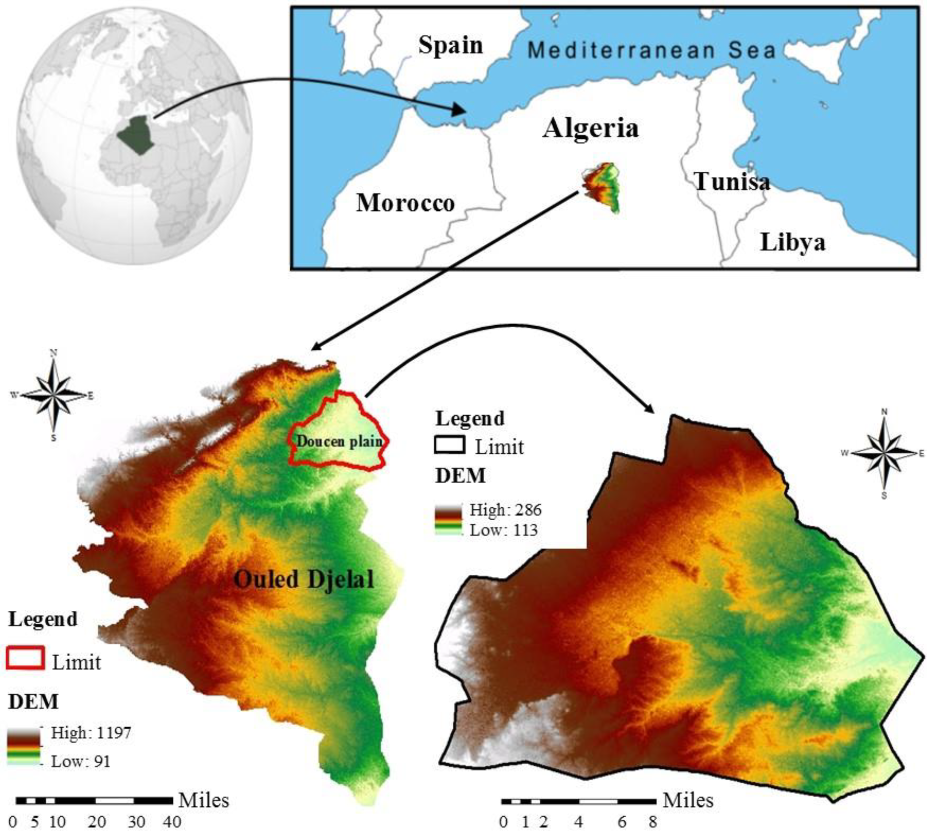
2.1. Study Area
2.2. Sampling and Hydrochemistry
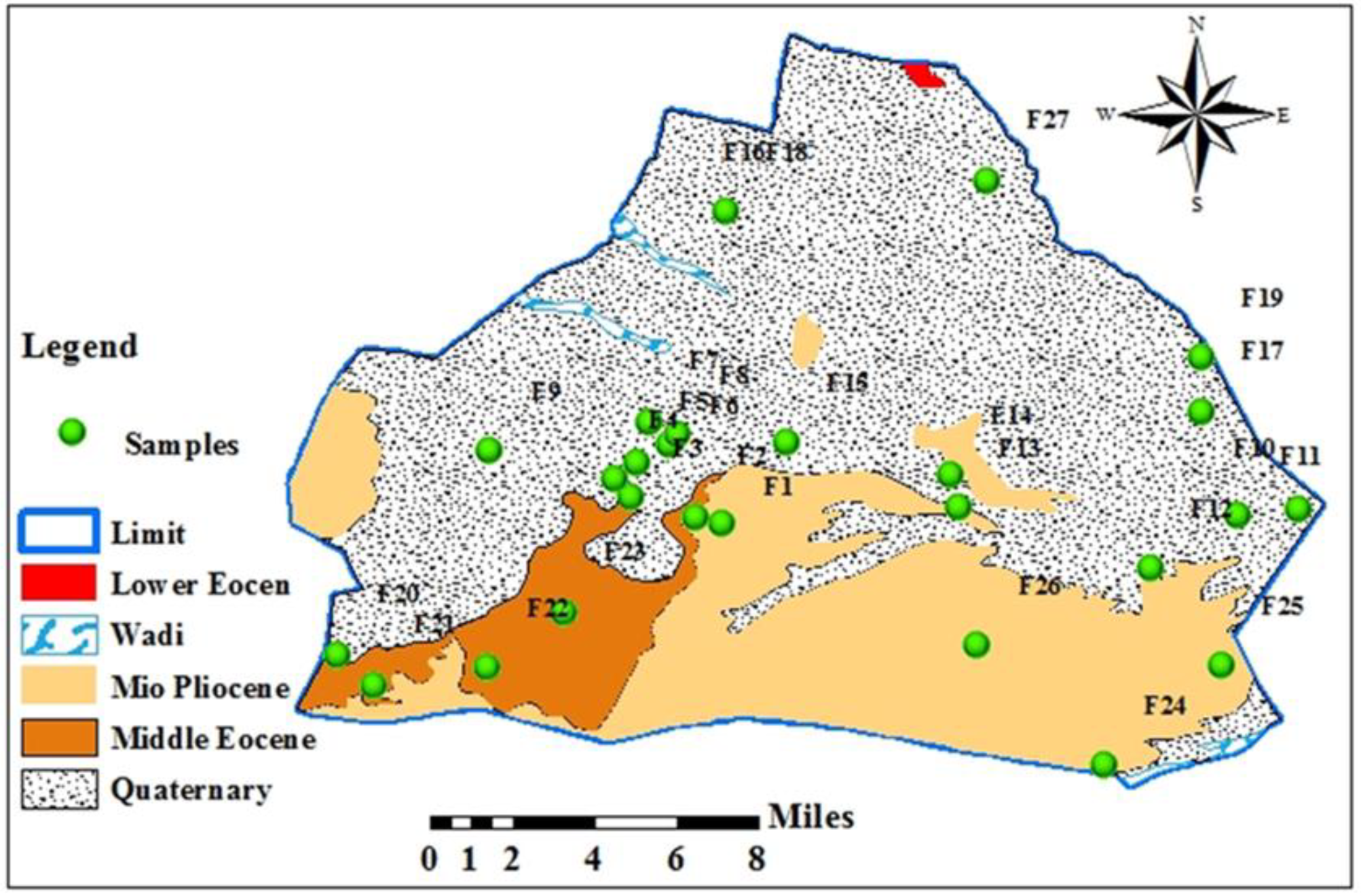
2.2.1. Samples Collection
2.2.2. Measurement of the Physicochemical Parameters
2.2.3. Multivariate Statistical Analysis for Data Treatment
2.3. Indexing Approaches
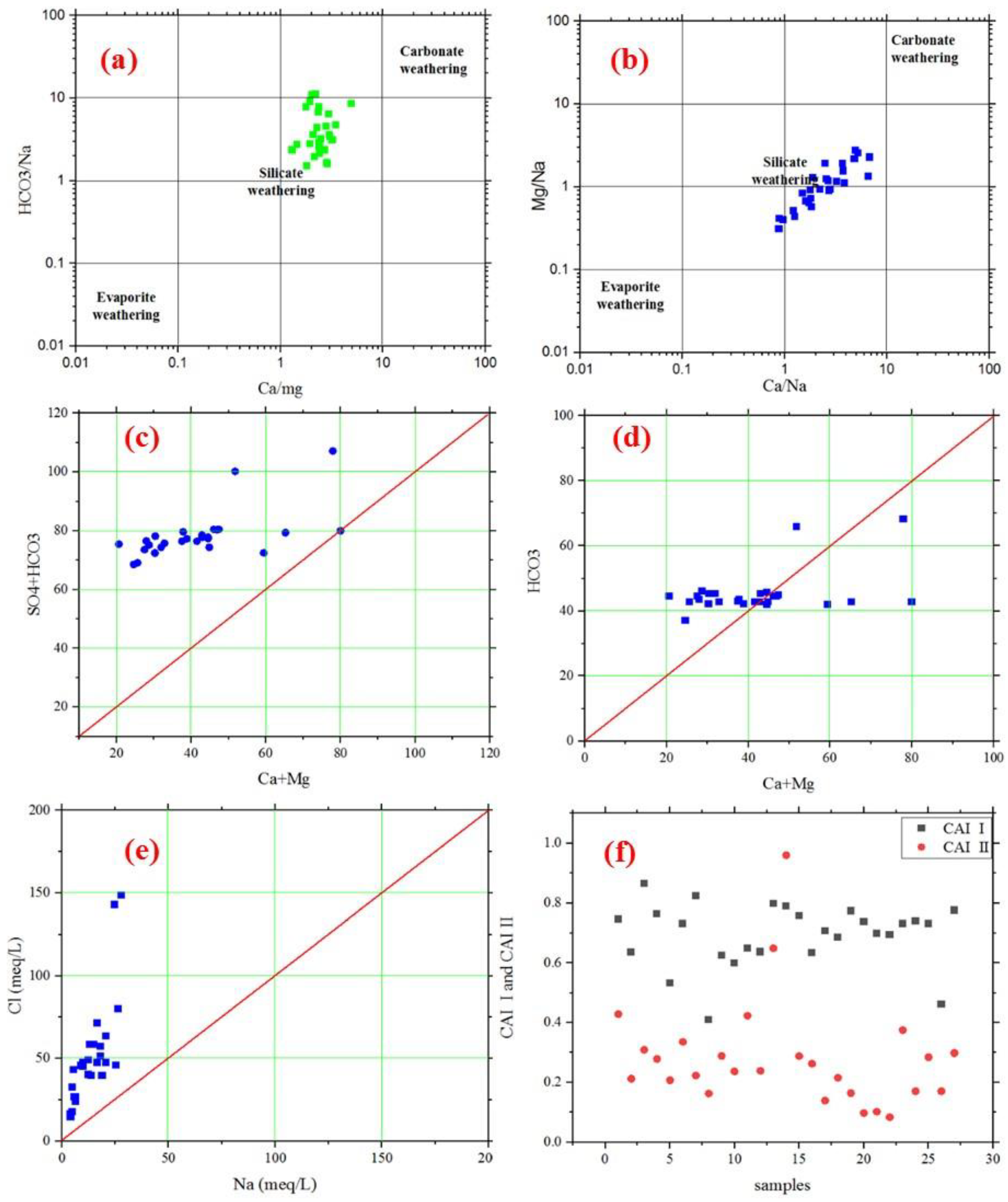
2.3.1. Chloro-Alkaline Indices (CAI 1 and CAI 2)
2.3.2. Irrigation Water Quality Indices (IWQIs)
2.4. Spatial Distribution Pattern
2.5. Gradient Boosting Regression (GBR)
2.6. Back-Propagation Neural Network (BPNN)
2.7. Datasets and Software for Data Analysis
2.8. Model Evaluation
3. Results and Discussion
3.1. Groundwater Hydrochemical Properties
3.2. Groundwater Facies and Source Identification
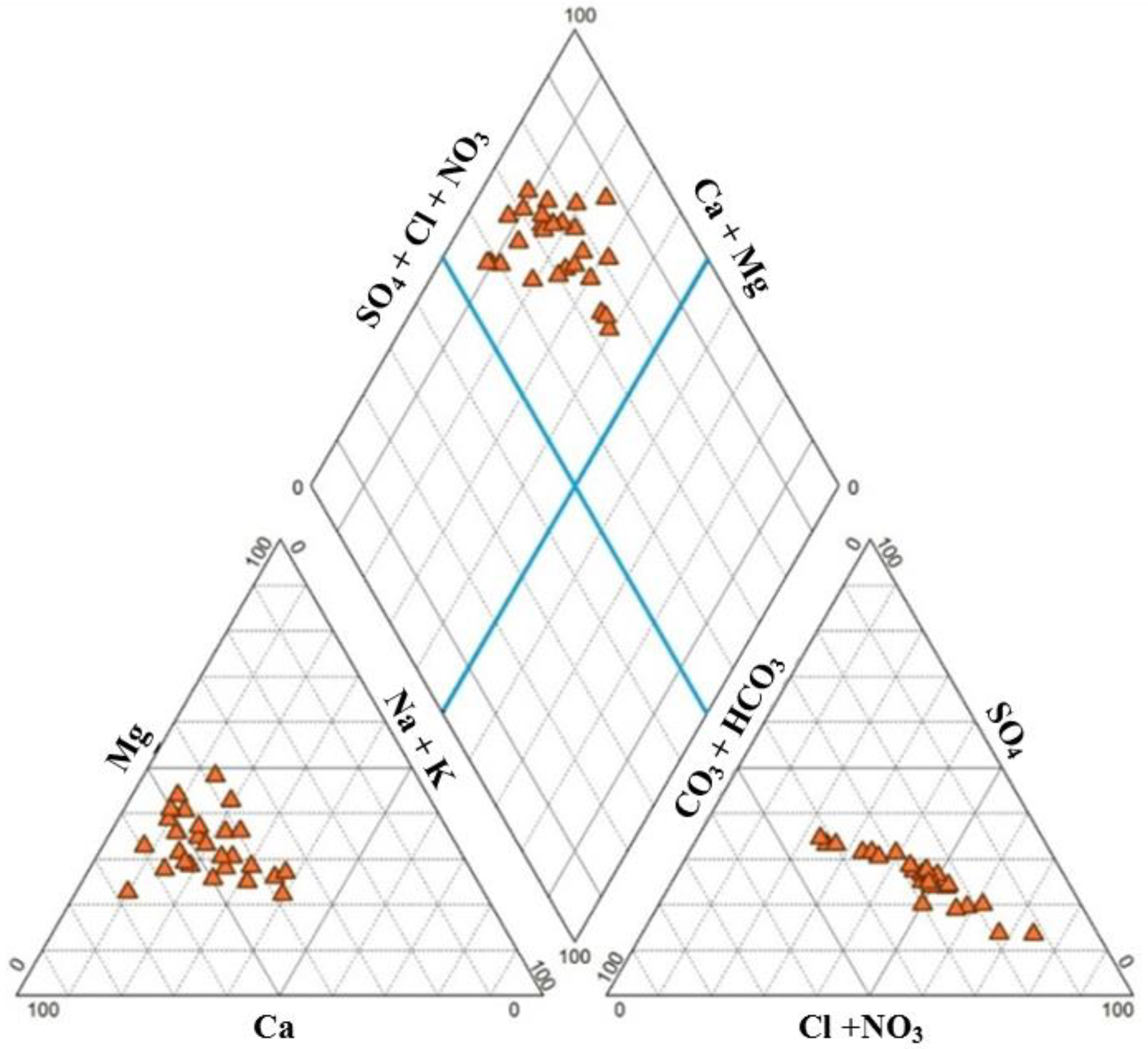
3.2.1. Groundwater Types
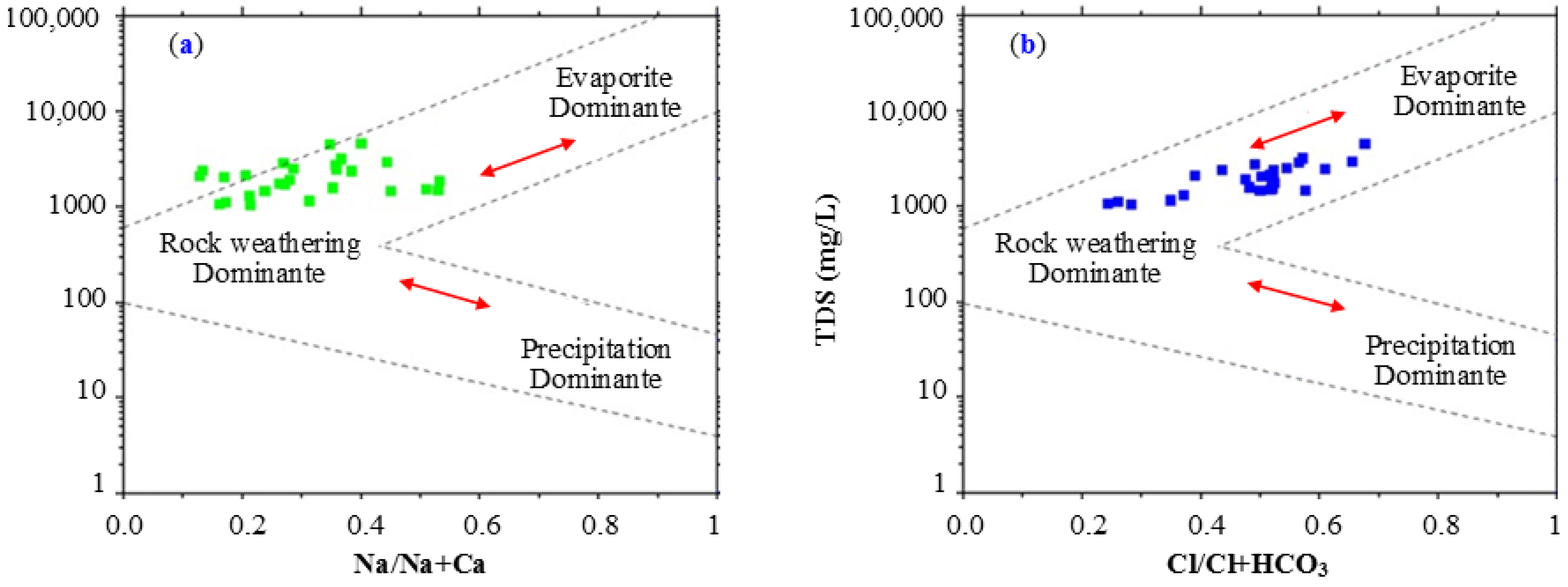
3.2.2. Processes Influencing Groundwater Chemistry
3.3. Analysis of Multivariate Statistics
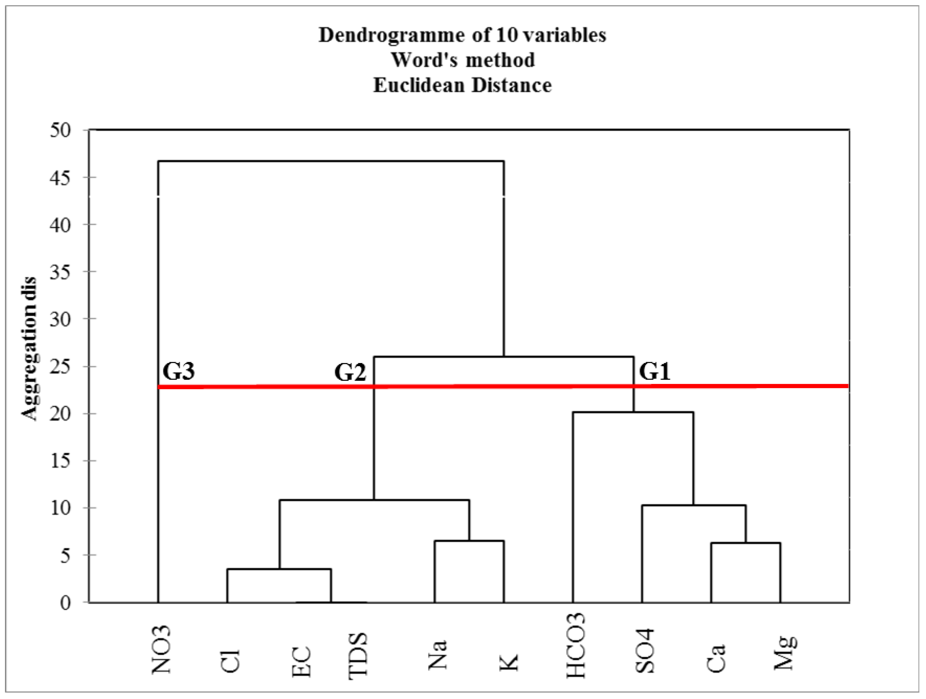
3.3.1. Cluster Analysis
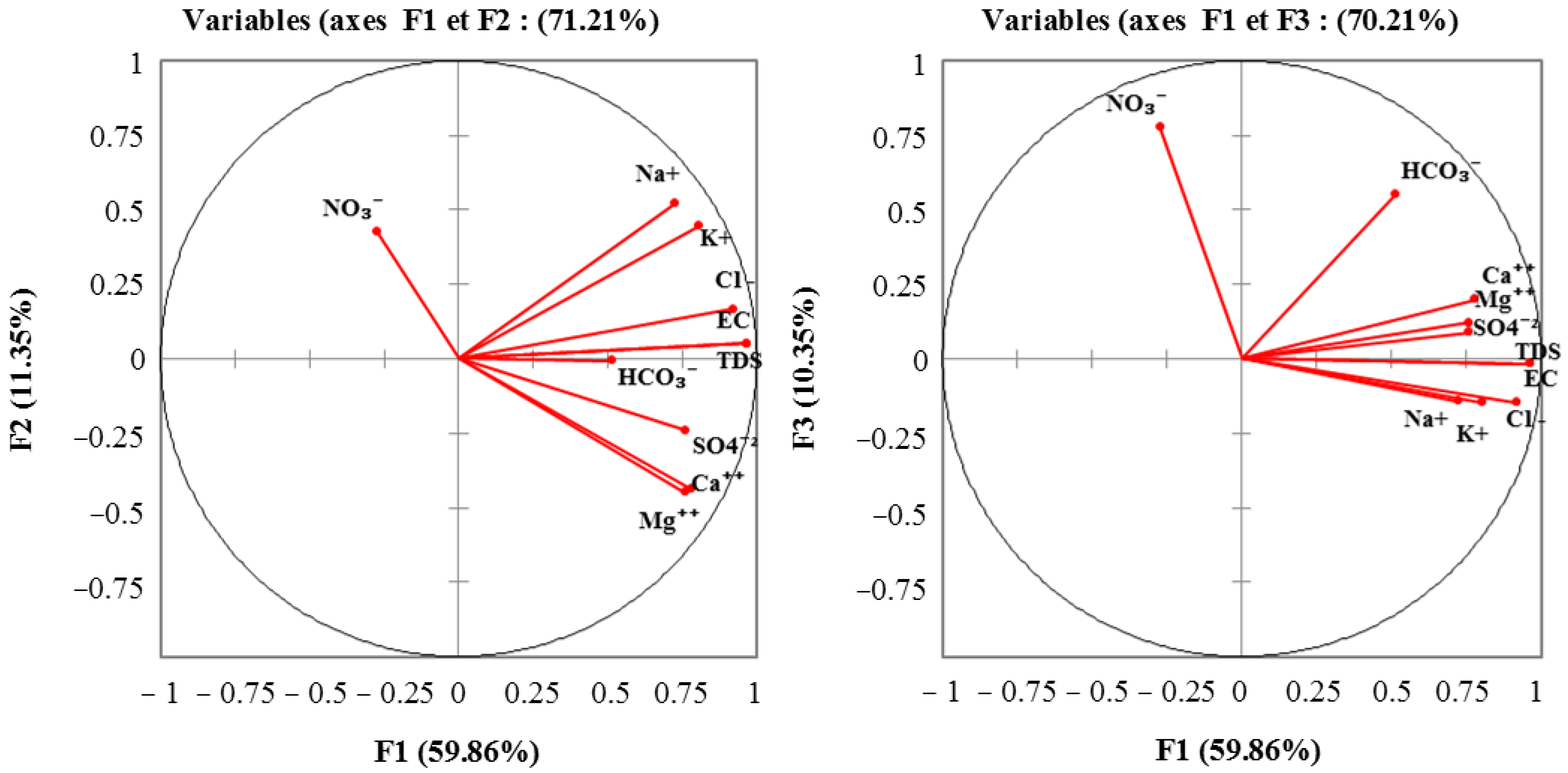
3.3.2. Principal Component Analysis (PCA)
3.4. Irrigation Water Quality Indices
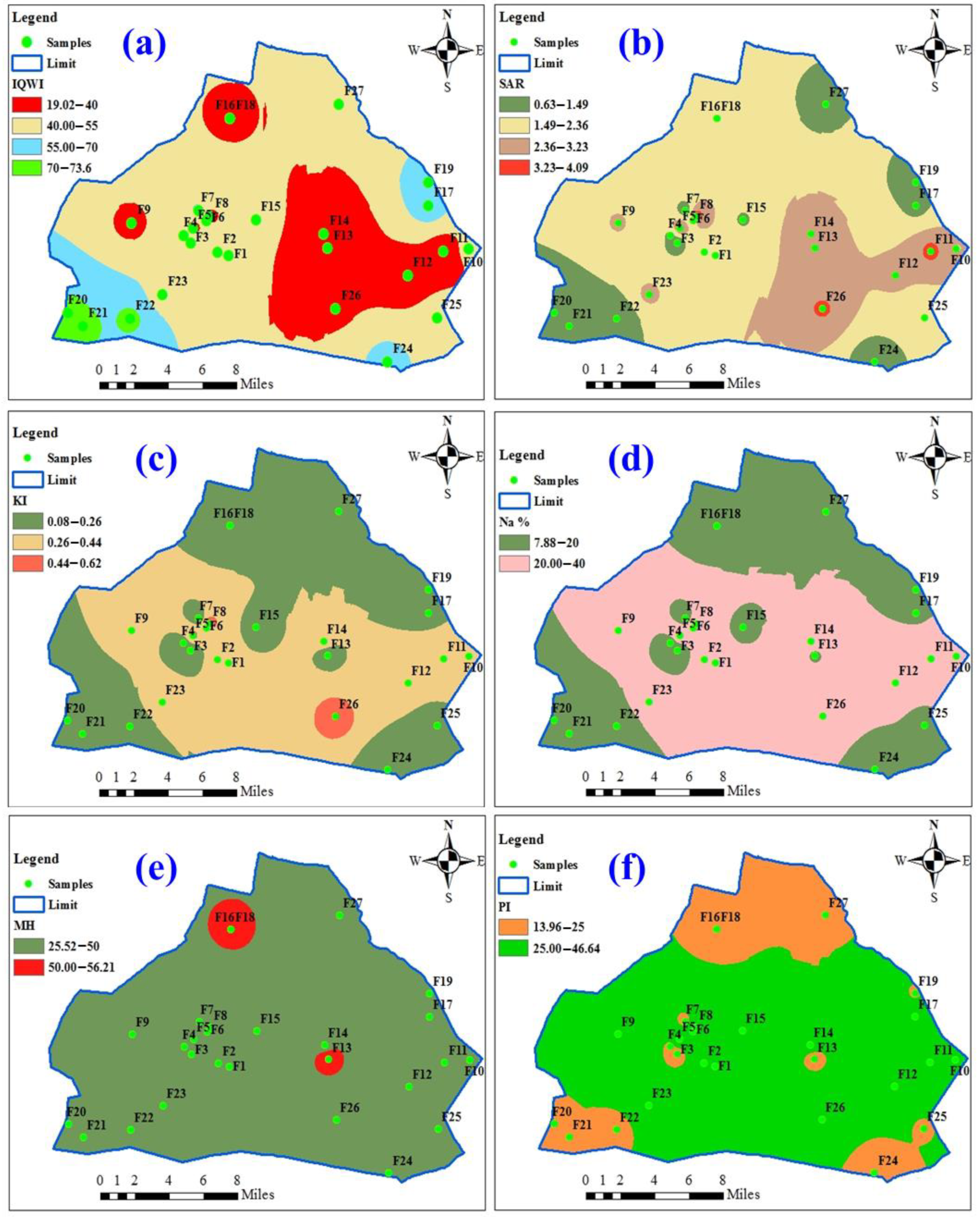
3.4.1. Irrigation Water Quality Index
3.4.2. Sodium Adsorption Ratio
3.4.3. Kelly Index
3.4.4. Sodium Percentage
3.4.5. Magnesium Hazards
3.4.6. Permeability Index
4. IWQIs Prediction Using GBR and ANN
5. Conclusions
Supplementary Materials
Author Contributions
Funding
Data Availability Statement
Acknowledgments
Conflicts of Interest
References
- Wada, Y.; van Beek, L.P.H.; van Kempen, C.M.; Reckman, J.W.T.M.; Vasak, S.; Bierkens, M.F.P. Global Depletion of Groundwater Resources: Global groundwater depletion. Geophys. Res. Lett. 2010, 37, L20402. [Google Scholar] [CrossRef]
- Naz, A.; Mishra, B.K.; Gupta, S.K. Human Health Risk Assessment of Chromium in Drinking Water: A Case Study of Sukinda Chromite Mine, Odisha, India. Expo Health 2016, 8, 253–264. [Google Scholar] [CrossRef]
- Gaagai, A. Etude de l’Evolution de la Qualité des Eaux du Barrage de Babar (Sud-Est Algérien) et l’Impact de la Rupture de la Digue sur l’Environnement. Ph.D. Thesis, University of Batna 2, Batna, Algeria, 2017. [Google Scholar] [CrossRef]
- Athamena, A.; Menani, M.R. Nitrogen Flux and Hydrochemical Characteristics of the Calcareous Aquifer of the Zana Plain, North East of Algeria. Arab. J. Geosci. 2018, 11, 356. [Google Scholar] [CrossRef]
- Koull, N.; Helimi, S.; Mihoub, A.; Mokhtari, S.; Kherraze, M.E.; Aouissi, H.A.; Koull, N.; Helimi, S.; Mihoub, A.; Mokhtari, S.; et al. Integración de SIG y Análisis Jerárquico Multi-Criterio Para Analizar La Idoneidad de La Tierra Para Los Cereales En La Zona Árida de Argelia. Int. J. Agric. Nat. Resour. 2022, 49, 36–50. [Google Scholar] [CrossRef]
- Belalite, H.; Menani, M.R.; Athamena, A. Calculation of Water Needs of the Main Crops and Water Resources Available in a Semi-Arid Climate, Case of Zana-Gadaïne Plain, Northeastern Algeria. Alger. J. Environ. Sci. Technol. 2022, 8, 2477–2488. [Google Scholar]
- Egbueri, J.C.; Ezugwu, C.K.; Unigwe, C.O.; Onwuka, O.S.; Onyemesili, O.C.; Mgbenu, C.N. Multidimensional Analysis of the Contamination Status, Corrosivity and Hydrogeochemistry of Groundwater from Parts of the Anambra Basin, Nigeria. Anal. Lett. 2021, 54, 2126–2156. [Google Scholar] [CrossRef]
- Noori, R.; Ghahremanzadeh, H.; Kløve, B.; Adamowski, J.F.; Baghvand, A. Modified-DRASTIC, modified-SINTACS and SI methods for groundwater vulnerability assessment in the southern Tehran aquifer. J. Environ. Sci. Health 2019, 54, 89–100. [Google Scholar] [CrossRef]
- Noori, R.; Maghrebi, M.; Mirchi, A.; Tang, Q.; Bhattarai, R.; Sadegh, M.; Nouryh, M.; Haghighia, A.T.; Kløvea, B.; Madani, K. Anthropogenic depletion of Iran’s aquifers. Proc. Natl. Acad. Sci. USA 2021, 118, e2024221118. [Google Scholar] [CrossRef]
- Maghrebi, M.; Noori, R.; Partani, S.; Araghi, A.; Barati, R.; Farnoush, H.; Haghighi, A.T. Iran’s groundwater hydrochemistry. Earth Space Sci. 2021, 8, e2021EA001793. [Google Scholar] [CrossRef]
- Ghodbane, M.; Benaabidate, L.; Boudoukha, A.; Gaagai, A.; Adjissi, O.; Chaib, W.; Aouissi, H.A. Analysis of groundwater quality in the lower Soummam Valley, North-East of Algeria. J. Water Land Dev. 2022, 54, 1–12. [Google Scholar] [CrossRef]
- Chorfi, A.; Hafid, H.; Baaloudj, A.; Rizi, H.; Aouissi, H.A.; Chaib, S.; Ababsa, M.; Allaoua, N.; Houhamdi, M. Characterization and Diversity of Macroin-Vertebrates in Groundwater in the Region of Souk-Ahras (North-East of Algeria). Ekológia 2022, 41, 219–227. [Google Scholar] [CrossRef]
- Şener, Ş.; Şener, E.; Davraz, A. Evaluation of Water Quality Using Water Quality Index (WQI) Method and GIS in Aksu River (SW-Turkey). Sci. Total Environ. 2017, 584–585, 131–144. [Google Scholar] [CrossRef]
- Elsayed, S.; Hussein, H.; Moghanm, F.S.; Khedher, K.M.; Eid, E.M.; Gad, M. Application of Irrigation Water Quality Indices and Multivariate Statistical Techniques for Surface Water Quality Assessments in the Northern Nile Delta, Egypt. Water 2020, 12, 3300. [Google Scholar] [CrossRef]
- El Osta, M.; Masoud, M.; Alqarawy, A.; Elsayed, S.; Gad, M. Groundwater Suitability for Drinking and Irrigation Using Water Quality Indices and Multivariate Modeling in Makkah Al-Mukarramah Province, Saudi Arabia. Water 2022, 14, 483. [Google Scholar] [CrossRef]
- Masoud, M.; El Osta, M.; Alqarawy, A.; Elsayed, S.; Gad, M. Evaluation of Groundwater Quality for Agricultural under Different Conditions Using Water Quality Indices, Partial Least Squares Regression Models, and GIS Approaches. Appl. Water Sci. 2022, 12, 244. [Google Scholar] [CrossRef]
- Gad, M.; El-Hendawy, S.; Al-Suhaibani, N.; Tahir, M.U.; Mubushar, M.; Elsayed, S. Combining Hydrogeochemical Characterization and a Hyperspectral Reflectance Tool for Assessing Quality and Suitability of Two Groundwater Resources for Irrigation in Egypt. Water 2020, 12, 2169. [Google Scholar] [CrossRef]
- Aouissi, H.A.; Ababsa, M.; Gaagai, A.; Bouslama, Z.; Farhi, Y.; Chenchouni, H. Does Melanin-Based Plumage Coloration Reflect Health Status of Free-Living Birds in Urban Environments? Avian Res. 2021, 12, 45. [Google Scholar] [CrossRef]
- Gad, M.; Abou El-Safa, M.M.; Farouk, M.; Hussein, H.; Alnemari, A.M.; Elsayed, S.; Khalifa, M.M.; Moghanm, F.S.; Eid, E.M.; Saleh, A.H. Integration of Water Quality Indices and Multivariate Modeling for Assessing Surface Water Quality in Qaroun Lake, Egypt. Water 2021, 13, 2258. [Google Scholar] [CrossRef]
- Nas, B.; Berktay, A. Groundwater Quality Mapping in Urban Groundwater Using GIS. Environ. Monit. Assess. 2010, 160, 215–227. [Google Scholar] [CrossRef]
- Gilbert, C.; Browell, J.; McMillan, D. Leveraging Turbine-Level Data for Improved Probabilistic Wind Power Forecasting. IEEE Trans. Sustain. Energy 2020, 11, 1152–1160. [Google Scholar] [CrossRef]
- Nayak, A.; Matta, G.; Uniyal, D.P. Hydrochemical Characterization of Groundwater Quality Using Chemometric Analysis and Water Quality Indices in the Foothills of Himalayas. Environ. Dev. Sustain. 2022, 1–32. [Google Scholar] [CrossRef] [PubMed]
- Vincevica-Gaile, Z.; Sachpazidou, V.; Bisters, V.; Klavins, M.; Anne, O.; Grinfelde, I.; Hanc, E.; Hogland, W.; Ibrahim, M.A.; Jani, Y.; et al. Applying Macroalgal Biomass as an Energy Source: Utility of the Baltic Sea Beach Wrack for Thermochemical Conversion. Sustainability 2022, 14, 13712. [Google Scholar] [CrossRef]
- Yotova, G.; Varbanov, M.; Tcherkezova, E.; Tsakovski, S. Water quality assessment of a river catchment by the composite water quality index and self-organizing maps. Ecol. Indic. 2021, 120, 106872. [Google Scholar] [CrossRef]
- Kebaili, F.K.; Baziz-Berkani, A.; Aouissi, H.A.; Mihai, F.-C.; Houda, M.; Ababsa, M.; Azab, M.; Petrisor, A.-I.; Fürst, C. Characterization and Planning of Household Waste Management: A Case Study from the MENA Region. Sustainability 2022, 14, 5461. [Google Scholar] [CrossRef]
- Varbanov, M.; Gartsiyanova, K.; Tcherkezova, E.; Kitev, A.; Genchev, S. Analysis of the quality of river water in Sofia city district, Bulgaria. J. Phys. Conf. Ser. 2021, 1960, 012019. [Google Scholar] [CrossRef]
- He, S.; Wu, J. Relationships of Groundwater Quality and Associated Health Risks with Land Use/Land Cover Patterns: A Case Study in a Loess Area, Northwest China. Hum. Ecol. Risk Assess. Int. J. 2019, 25, 354–373. [Google Scholar] [CrossRef]
- Gad, M.; Saleh, A.H.; Hussein, H.; Farouk, M.; Elsayed, S. Appraisal of Surface Water Quality of Nile River Using Water Quality Indices, Spectral Signature and Multivariate Modeling. Water 2022, 14, 1131. [Google Scholar] [CrossRef]
- Khadr, M.; Gad, M.; El-Hendawy, S.; Al-Suhaibani, N.; Dewir, Y.H.; Tahir, M.U.; Mubushar, M.; Elsayed, S. The Integration of Multivariate Statistical Approaches, Hyperspectral Reflectance, and Data-Driven Modeling for Assessing the Quality and Suitability of Groundwater for Irrigation. Water 2021, 13, 35. [Google Scholar] [CrossRef]
- Eid, M.H.; Elbagory, M.; Tamma, A.A.; Gad, M.; Elsayed, S.; Hussein, H.; Moghanm, F.S.; Omara, A.E.-D.; Kovács, A.; Péter, S. Evaluation of Groundwater Quality for Irrigation in Deep Aquifers Using Multiple Graphical and Indexing Approaches Supported with Machine Learning Models and GIS Techniques, Souf Valley, Algeria. Water 2023, 15, 182. [Google Scholar] [CrossRef]
- Schulze, F.H.; Wolf, H.; Jansen, H.W.; van der Veer, P. Applications of Artificial Neural Networks in Integrated Water Management: Fiction or Future? Water Sci. Technol. 2005, 52, 21–31. [Google Scholar] [CrossRef]
- Strobl, C.; Boulesteix, A.-L.; Kneib, T.; Augustin, T.; Zeileis, A. Conditional Variable Importance for Random Forests. BMC Bioinform. 2008, 9, 307. [Google Scholar] [CrossRef]
- Glorfeld, L. A Methodology for Simplification and Interpretation of Backpropagation-Based Neural Network Models. Expert Syst. Appl. 1996, 10, 37–54. [Google Scholar] [CrossRef]
- Melis, G.; Dyer, C.; Blunsom, P. On the State of the Art of Evaluation in Neural Language Models. arXiv 2017, arXiv:1707.05589. [Google Scholar]
- Bergstra, J.; Yamins, D.; Cox, D. Making a Science of Model Search: Hyperparameter Optimization in Hundreds of Dimensions for Vision Architectures. In Proceedings of the 30th International Conference on Machine Learning, Atlanta, GA, USA, 16–21 June 2013; Dasgupta, S., McAllester, D., Eds.; Volume 28, pp. 115–123. [Google Scholar]
- Wu, J.; Chen, X.-Y.; Zhang, H.; Xiong, L.-D.; Lei, H.; Deng, S.-H. Hyperparameter Optimization for Machine Learning Models Based on Bayesian Optimizationb. J. Electron. Sci. Technol. 2019, 17, 26–40. [Google Scholar] [CrossRef]
- Gad, M.; El Osta, M. Geochemical Controlling Mechanisms and Quality of the Groundwater Resources in El Fayoum Depression, Egypt. Arab. J. Geosci. 2020, 13, 861. [Google Scholar] [CrossRef]
- Gul, S.; Gul, H.; Gul, M.; Khattak, R.; Rukh, G.; Khan, M.S.; Aouissi, H.A. Enhanced Adsorption of Rhodamine B on Biomass of Cypress/False Cypress (Chamaecyparis lawsoniana) Fruit: Optimization and Kinetic Study. Water 2022, 14, 2987. [Google Scholar] [CrossRef]
- Bencer, S.; Boudoukha, A.; Mouni, L. Multivariate Statistical Analysis of the Groundwater of Ain Djacer Area (Eastern of Algeria). Arab. J. Geosci. 2016, 9, 248. [Google Scholar] [CrossRef]
- Eaton, A.D.; Clesceri, L.S.; Rice, E.W.; Greenberg, A.E.; Franson, A.H. (Eds.) Standard Methods for the Examination of Water & Wastewater, 21st ed.; Amer Public Health Association: Washington, DC, USA, 2005. [Google Scholar]
- Gaagai, A.; Boudoukha, A.; Boumezbeur, A.; Benaabidate, L. Hydrochemical Characterization of Surface Water in the Babar Watershed (Algeria) Using Environmetric Techniques and Time Series Analysis. Int. J. River Basin Manag. 2017, 15, 361–372. [Google Scholar] [CrossRef]
- Gad, M.; Elsayed, S.; Moghanm, F.S.; Almarshadi, M.H.; Alshammari, A.S.; Khedher, K.M.; Eid, E.M.; Hussein, H. Combining Water Quality Indices and Multivariate Modeling to Assess Surface Water Quality in the Northern Nile Delta, Egypt. Water 2020, 12, 2142. [Google Scholar] [CrossRef]
- Belkhiri, L.; Boudoukha, A.; Mouni, L.; Baouz, T. Application of Multivariate Statistical Methods and Inverse Geochemical Modeling for Characterization of Groundwater—A Case Study: Ain Azel Plain (Algeria). Geoderma 2010, 159, 390–398. [Google Scholar] [CrossRef]
- Hinge, G.; Bharali, B.; Baruah, A.; Sharma, A. Integrated Groundwater Quality Analysis Using Water Quality Index, GIS and Multivariate Technique: A Case Study of Guwahati City. Environ. Earth Sci. 2022, 81, 412. [Google Scholar] [CrossRef]
- Kaiser, H.F. The Varimax Criterion for Analytic Rotation in Factor Analysis. Psychometrika 1958, 23, 187–200. [Google Scholar] [CrossRef]
- Schoeller, H. Methods and Techniques of Groundwater Investigation and Development. Water Resour. Ser. 1967, 33, 44–52. [Google Scholar]
- Meireles, A.C.M.; de Andrade, E.M.; Chaves, L.C.G.; Frischkorn, H.; Crisostomo, L.A. A New Proposal of the Classification of Irrigation Water. Rev. Ciênc. Agron. 2010, 41, 349–357. [Google Scholar] [CrossRef]
- Oster, J.D.; Sposito, G. The Gapon Coefficient and the Exchangeable Sodium Percentage-Sodium Adsorption Ratio Relation. Soil Sci. Soc. Am. J. 1980, 44, 258–260. [Google Scholar] [CrossRef]
- Srinivasamoorthy, K.; Gopinath, M.; Chidambaram, S.; Vasanthavigar, M.; Sarma, V.S. Hydrochemical Characterization and Quality Appraisal of Groundwater from Pungar Sub Basin, Tamilnadu, India. J. King Saud Univ. Sci. 2014, 26, 37–52. [Google Scholar] [CrossRef]
- Ravikumar, P.; Aneesul Mehmood, M.; Somashekar, R.K. Water Quality Index to Determine the Surface Water Quality of Sankey Tank and Mallathahalli Lake, Bangalore Urban District, Karnataka, India. Appl. Water Sci. 2013, 3, 247–261. [Google Scholar] [CrossRef]
- Zhang, T.; Cai, W.; Li, Y.; Geng, T.; Zhang, Z.; Lv, Y.; Zhao, M.; Liu, J. Ion Chemistry of Groundwater and the Possible Controls within Lhasa River Basin, SW Tibetan Plateau. Arab. J. Geosci. 2018, 11, 510. [Google Scholar] [CrossRef]
- Das, S.; Nag, S.K. Deciphering Groundwater Quality for Irrigation and Domestic Purposes—A Case Study in Suri I and II Blocks, Birbhum District, West Bengal, India. J. Earth Syst. Sci. 2015, 124, 965–992. [Google Scholar] [CrossRef]
- Elith, J.; Leathwick, J.R.; Hastie, T. A Working Guide to Boosted Regression Trees. J. Anim. Ecol. 2008, 77, 802–813. [Google Scholar] [CrossRef]
- Schalkoff, R.J. Artificial Neural Networks; McGraw-Hill Higher Education: New York, NY, USA, 1997; ISBN 0-07-057118-X. [Google Scholar]
- Haykin, S. Self-Organizing Maps. Neural Netw. Compr. Found. 1999, 2, 443–483. [Google Scholar]
- Li, J.; Yoder, R.E.; Odhiambo, L.O.; Zhang, J. Simulation of Nitrate Distribution under Drip Irrigation Using Artificial Neural Networks. Irrig. Sci. 2004, 23, 29–37. [Google Scholar] [CrossRef]
- Byrd, R.H.; Lu, P.; Nocedal, J.; Zhu, C. A Limited Memory Algorithm for Bound Constrained Optimization. SIAM J. Sci. Comput. 1995, 16, 1190–1208. [Google Scholar] [CrossRef]
- Noori, R.; Karbassi, A.R.; Mehdizadeh, H.; Vesali-Naseh, M.; Sabahi, M.S. A framework development for predicting the longitudinal dispersion coefficient in natural streams using an artificial neural network. Environ. Prog. Sustain. Energy 2011, 30, 439–449. [Google Scholar] [CrossRef]
- Zhu, J.; Huang, Z.; Sun, H.; Wang, G. Mapping Forest Ecosystem Biomass Density for Xiangjiang River Basin by Combining Plot and Remote Sensing Data and Comparing Spatial Extrapolation Methods. Remote Sens. 2017, 9, 241. [Google Scholar] [CrossRef]
- Malone, B.P.; Styc, Q.; Minasny, B.; McBratney, A.B. Digital Soil Mapping of Soil Carbon at the Farm Scale: A Spatial Downscaling Approach in Consideration of Measured and Uncertain Data. Geoderma 2017, 290, 91–99. [Google Scholar] [CrossRef]
- Saggi, M.K.; Jain, S. Reference Evapotranspiration Estimation and Modeling of the Punjab Northern India Using Deep Learning. Comput. Electron. Agric. 2019, 156, 387–398. [Google Scholar] [CrossRef]
- Lakshmanan, E.; Kannan, R.; Senthil Kumar, M. Major Ion Chemistry and Identification of Hydrogeochemical Processes of Ground Water in a Part of Kancheepuram District, Tamil Nadu, India. Environ. Geosci. 2003, 10, 157–166. [Google Scholar] [CrossRef]
- Ayers, R.; Westcott, D. Water Quality for Agriculture. FAO Irrigation and Drainage; Paper 29 Revision 1; Food and Agricultural Organization of the United Nations: Rome, Italy, 1994. [Google Scholar]
- Athamena, A.; Gaagai, A.; Aouissi, H.A.; Burlakovs, J.; Bencedira, S.; Zekker, I.; Krauklis, A.E. Chemometrics of the Environment: Hydrochemical Characterization of Groundwater in Lioua Plain (North Africa) Using Time Series and Multivariate Statistical Analysis. Sustainability 2023, 15, 20. [Google Scholar] [CrossRef]
- Gaagai, A.; Aouissi, H.A.; Krauklis, A.E.; Burlakovs, J.; Athamena, A.; Zekker, I.; Boudoukha, A.; Benaabidate, L.; Chenchouni, H. Modeling and Risk Analysis of Dam-Break Flooding in a Semi-Arid Montane Watershed: A Case Study of the Yabous Dam, Northeastern Algeria. Water 2022, 14, 767. [Google Scholar] [CrossRef]
- Ghalib, H.B. Groundwater Chemistry Evaluation for Drinking and Irrigation Utilities in East Wasit Province, Central Iraq. Appl. Water Sci. 2017, 7, 3447–3467. [Google Scholar] [CrossRef]
- Tang, H.; Zhong, H.; Pan, Y.; Zhou, Q.; Huo, Z.; Chu, W.; Xu, B. A New Group of Heterocyclic Nitrogenous Disinfection Byproducts (DBPs) in Drinking Water: Role of Extraction PH in Unknown DBP Exploration. Environ. Sci. Technol. 2021, 55, 6764–6772. [Google Scholar] [CrossRef]
- Selvam, S.; Venkatramanan, S.; Chung, S.Y.; Singaraja, C. Identification of Groundwater Contamination Sources in Dindugal District of Tamil Nadu, India Using GIS and Multivariate Statistical Analyses. Arab. J. Geosci. 2016, 9, 407. [Google Scholar] [CrossRef]
- Litvinovich, A.; Pavlova, O.; Lavrishchev, A.; Bure, V.; Saljnikov, E. Magnesium Leaching Processes from Sod-Podzolic Sandy Loam Reclaimed by Increasing Doses of Finely Ground Dolomite. Zemdirb. Agric. 2021, 108, 109–116. [Google Scholar] [CrossRef]
- Guerzou, M.; Aouissi, H.A.; Guerzou, A.; Burlakovs, J.; Doumandji, S.; Krauklis, A.E. From the Beehives: Identification and Comparison of Physicochemical Properties of Algerian Honey. Resources 2021, 10, 94. [Google Scholar] [CrossRef]
- Piper, A.M. A Graphic Procedure in the Geochemical Interpretation of Water-Analyses. Trans. AGU 1944, 25, 914. [Google Scholar] [CrossRef]
- Alqarawy, A.; El Osta, M.; Masoud, M.; Elsayed, S.; Gad, M. Use of Hyperspectral Reflectance and Water Quality Indices to Assess Groundwater Quality for Drinking in Arid Regions, Saudi Arabia. Water 2022, 14, 2311. [Google Scholar] [CrossRef]
- Gibbs, R.J. Mechanisms Controlling World Water Chemistry. Science 1970, 170, 1088–1090. [Google Scholar] [CrossRef]
- Ghahremanzadeh, H.; Noori, R.; Baghvand, A.; Nasrabadi, T. Evaluating the main sources of groundwater pollution in the southern Tehran aquifer using principal component factor analysis. Environ. Geochem. Health 2018, 40, 1317–1328. [Google Scholar] [CrossRef]
- Wu, J.; Li, P.; Qian, H. Hydrochemical Characterization of Drinking Groundwater with Special Reference to Fluoride in an Arid Area of China and the Control of Aquifer Leakage on Its Concentrations. Environ. Earth Sci. 2015, 73, 8575–8588. [Google Scholar] [CrossRef]
- Mukherjee, A.; Fryar, A.E.; Scanlon, B.R.; Bhattacharya, P.; Bhattacharya, A. Elevated Arsenic in Deeper Groundwater of the Western Bengal Basin, India: Extent and Controls from Regional to Local Scale. Appl. Geochem. 2011, 26, 600–613. [Google Scholar] [CrossRef]
- Diwakar, J.; Johnston, S.G.; Burton, E.D.; Shrestha, S.D. Arsenic Mobilization in an Alluvial Aquifer of the Terai Region, Nepal. J. Hydrol. Reg. Stud. 2015, 4, 59–79. [Google Scholar] [CrossRef]
- Kumar, S.; Kumar, A.; Prashant; Jha, V.N.; Sahoo, S.K.; Ranjan, R.K. Groundwater Quality and Its Suitability for Drinking and Irrigational Purpose in Bhojpur District: Middle Gangetic Plain of Bihar, India. Water Supply 2022, 22, 7072–7084. [Google Scholar] [CrossRef]
- Islam, J.; Hossain, A.M.; Rahman, S.; Khandoker, H.; Zahan, M.N. Hydrogeochemistry and Usability of Groundwater at the Tista River Basin in Northern Bangladesh. Indian J. Sci. Technol. 2019, 12, 1–12. [Google Scholar] [CrossRef]
- Qian, C.; Wu, X.; Mu, W.-P.; Fu, R.-Z.; Zhu, G.; Wang, Z.-R.; Wang, D. Hydrogeochemical Characterization and Suitability Assessment of Groundwater in an Agro-Pastoral Area, Ordos Basin, NW China. Environ. Earth Sci. 2016, 75, 1356. [Google Scholar] [CrossRef]
- Noori, R.; Berndtsson, R.; Hosseinzadeh, M.; Adamowski, J.F.; Abyaneh, M.R. A critical review on the application of the National Sanitation Foundation Water Quality Index. Environ. Pollut. 2019, 244, 575–587. [Google Scholar] [CrossRef]
- Güler, C.; Thyne, G.D.; McCray, J.E.; Turner, K.A. Evaluation of Graphical and Multivariate Statistical Methods for Classification of Water Chemistry Data. Hydrogeol. J. 2002, 10, 455–474. [Google Scholar] [CrossRef]
- Kawo, N.S.; Karuppannan, S. Groundwater Quality Assessment Using Water Quality Index and GIS Technique in Modjo River Basin, Central Ethiopia. J. Afr. Earth Sci. 2018, 147, 300–311. [Google Scholar] [CrossRef]
- Li, P.; Wu, J.; Qian, H. Assessment of Groundwater Quality for Irrigation Purposes and Identification of Hydrogeochemical Evolution Mechanisms in Pengyang County, China. Environ. Earth Sci. 2013, 69, 2211–2225. [Google Scholar] [CrossRef]
- Noori, R.; Hooshyaripor, F.; Javadi, S.; Dodangeh, M.; Tian, F.; Adamowski, J.F.; Berndtsson, R.; Baghvand, A.; Klöve, B. PODMT3DMS-Tool: Proper orthogonal decomposition linked to the MT3DMS model for nitrate simulation in aquifers. Hydrogeol. J. 2020, 28, 1125–1142. [Google Scholar] [CrossRef]
- RamyaPriya, R.; Elango, L. Evaluation of Geogenic and Anthropogenic Impacts on Spatio-Temporal Variation in Quality of Surface Water and Groundwater along Cauvery River, India. Environ. Earth Sci. 2018, 77, 2. [Google Scholar] [CrossRef]
- Elsayed, S.; Ibrahim, H.; Hussein, H.; Elsherbiny, O.; Elmetwalli, A.H.; Moghanm, F.S.; Ghoneim, A.M.; Danish, S.; Datta, R.; Gad, M. Assessment of Water Quality in Lake Qaroun Using Ground-Based Remote Sensing Data and Artificial Neural Networks. Water 2021, 13, 3094. [Google Scholar] [CrossRef]
- Wang, X.; Ozdemir, O.; Hampton, M.A.; Nguyen, A.V.; Do, D.D. The Effect of Zeolite Treatment by Acids on Sodium Adsorption Ratio of Coal Seam Gas Water. Water Res. 2012, 46, 5247–5254. [Google Scholar] [CrossRef]
- Hanson, B.; Grattan, S.R.; Fulton, A. Agricultural Salinity and Drainage; Irrigation Program, University of California: Davis, CA, USA, 1999. [Google Scholar]
- Sudhakar, A.; Narsimha, A. Suitability and Assessment of Groundwater for Irrigation Purpose: A Case Study of Kushaiguda Area, Ranga Reddy District, Andhra Pradesh, India. Adv. Appl. Sci. Res. 2013, 4, 75–81. [Google Scholar]
- Kelley, W.P. Permissible Composition and Concentration of Irrigation Water. Proc. Am. Soc. Civil Eng. 1940, 66, 607–613. [Google Scholar] [CrossRef]
- Sundaray, S.K.; Nayak, B.B.; Bhatta, D. Environmental Studies on River Water Quality with Reference to Suitability for Agricultural Purposes: Mahanadi River Estuarine System, India—A Case Study. Environ. Monit. Assess. 2009, 155, 227–243. [Google Scholar] [CrossRef]
- Todd, D.K.; Mays, L.W. Groundwater Hydrology; John Wiley & Sons: Hoboken, NJ, USA, 2004; ISBN 0-471-05937-4. [Google Scholar]
- Wilcox, L.V. The Quality of Water for Irrigation Use; Technical Bulletin; US Government Printing Office: Washington, DC, USA, 1948; 19p. [Google Scholar]
- Paliwal, K.V. Irrigation with Saline Water; Water Technology Centre, Indian Agriculture Research Institute: New Delhi, India, 1972. [Google Scholar]
- Doneen, L.D. Water Quality for Agriculture, Department of Irrigation; University of California: Davis, CA, USA, 1964; p. 48. [Google Scholar]
- Elsherbiny, O.; Zhou, L.; Feng, L.; Qiu, Z. Integration of Visible and Thermal Imagery with an Artificial Neural Network Approach for Robust Forecasting of Canopy Water Content in Rice. Remote Sens. 2021, 13, 1785. [Google Scholar] [CrossRef]
- Elsherbiny, O.; Zhou, L.; He, Y.; Qiu, Z. A Novel Hybrid Deep Network for Diagnosing Water Status in Wheat Crop Using IoT-Based Multimodal Data. Comput. Electron. Agric. 2022, 203, 107453. [Google Scholar] [CrossRef]


| WQIs | Formula | References |
|---|---|---|
| IWQI | [47] | |
| SAR | [48] | |
| KI | [49] | |
| Na% | [50] | |
| MH | [51] | |
| PI | [52] |
| Parameters | FAO * | Minimum | Maximum | Average | Standard Deviation |
|---|---|---|---|---|---|
| pH | 8.5 | 7.08 | 8.24 | 7.50 | 0.24 |
| TDS | 2000 | 1046 | 4650 | 2137 | 931 |
| EC | 3000 | 2091 | 9300 | 4274 | 1862 |
| K+ | 2 | 2.00 | 50.00 | 16.89 | 13.20 |
| Na+ | 919 | 50.00 | 340.00 | 167.11 | 89.98 |
| Ca2+ | 400 | 176.00 | 561.00 | 353.48 | 110.30 |
| Mg2+ | 60 | 75.00 | 423.00 | 155.44 | 84.31 |
| SO42− | 960 | 320.00 | 472.00 | 403.26 | 36.17 |
| Cl− | 1036 | 177.00 | 1808.00 | 621.67 | 384.37 |
| HCO3− | 610 | 450.00 | 830.00 | 548.81 | 79.74 |
| NO3− | 10 | 3.61 | 41.80 | 19.18 | 10.94 |
| Parameter | F1 | F2 | F3 |
|---|---|---|---|
| EC | 0.965 | 0.051 | −0.016 |
| TDS | 0.965 | 0.051 | −0.016 |
| Ca2+ | 0.781 | −0.438 | 0.200 |
| Mg2+ | 0.761 | −0.448 | 0.121 |
| HCO₃− | 0.514 | −0.007 | 0.551 |
| Cl− | 0.920 | 0.166 | −0.148 |
| Na+ | 0.724 | 0.522 | −0.141 |
| K+ | 0.805 | 0.444 | −0.147 |
| SO42− | 0.761 | −0.241 | 0.089 |
| NO3− | −0.274 | 0.427 | 0.778 |
| Criteria | Min | Max | Mean | Range | Class | Number of Samples (%) |
|---|---|---|---|---|---|---|
| IWQI | 19.01 | 73.61 | 47.17 | 85–100 | No restriction | 0 (0.0%) |
| 70–85 | Low restriction | 0 (0.0%) | ||||
| 55–70 | Moderate restriction | 9 (33.33%) | ||||
| 40–55 | High restriction | 9 (33.33%) | ||||
| 0–40 | Severe restriction | 9 (33.33%) | ||||
| SAR | 0.63 | 4.10 | 1.88 | <10 | Excellent | 27 (100%) |
| 10–18 | Good | 0.00 | ||||
| 19–26 | Fair Poor | 0.00 | ||||
| >26 | Unsuitable | 0.00 | ||||
| KI | 0.08 | 0.62 | 0.25 | <1 | Suitable | 27 (100%) |
| >1 | Unsuitable | 0.00 | ||||
| Na% | 7.88 | 39.31 | 19.96 | <20% | Excellent | 16 (59.26%) |
| 21–40% | Good | 11 (40.74%) | ||||
| 41–60% | Permissible | 0.00 | ||||
| 61–80% | Doubtful | 0.00 | ||||
| >80% | Unsuitable | 0.00 | ||||
| MH | 25.38 | 56.22 | 41.18 | <50% | Suitable | 25 (92.59%) |
| >50% | Unsuitable | 2 (7.41%) | ||||
| PI | 13.95 | 46.68 | 27.87 | >75% | Suitable | 0.00 |
| 25–75% | Moderate | 15 (55.55%) | ||||
| <25% | Unsuitable | 12 (44.44%) |
| Variable | Model | Optimal Features (F) | Hyper-Parameters | Training | Validation | ||
|---|---|---|---|---|---|---|---|
| R2 | RMSE | R2 | RMSE | ||||
| IWQI | GBR | EC, Na+, Cl− | (Ns = 25, Mf = log2) | 0.991 | 1.481 | 0.951 | 2.562 |
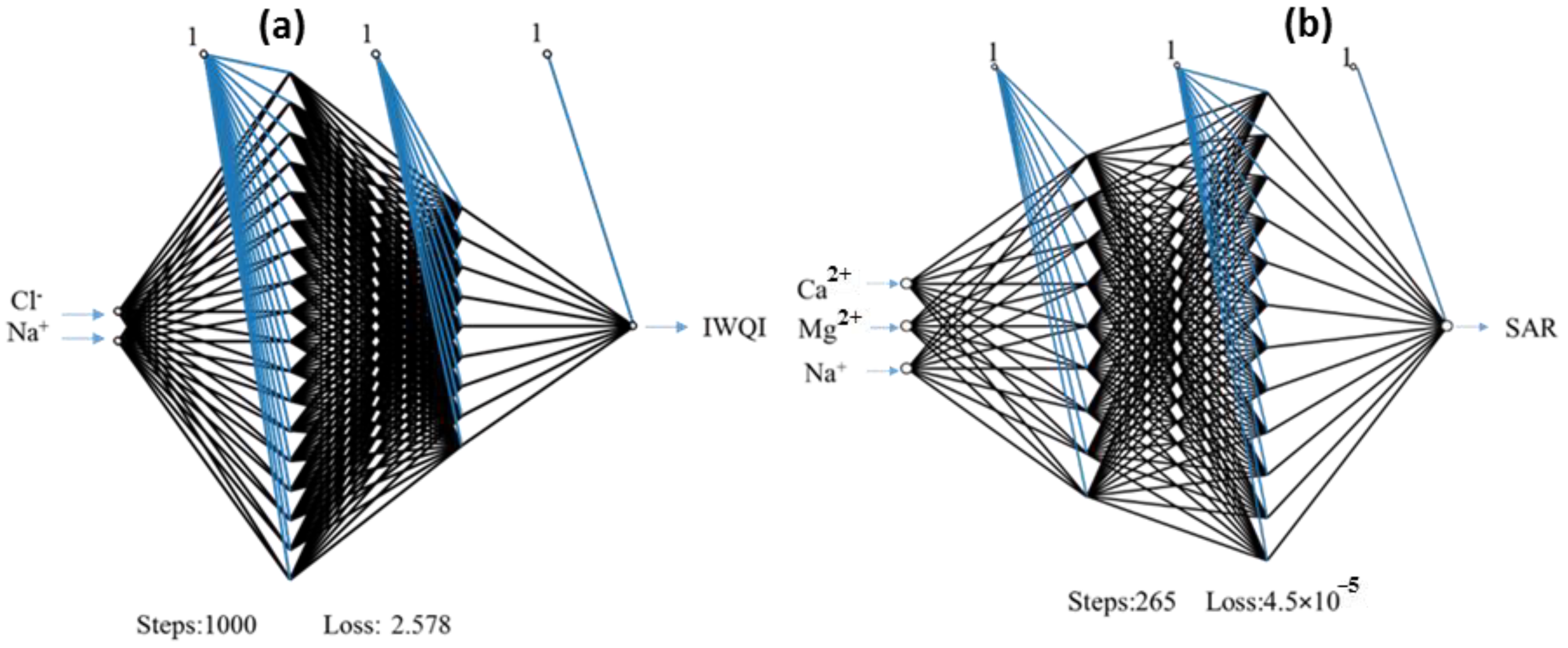
| ANN | Cl−, Na+ | (h1 = 18, h2 = 9, fun = relu) | 0.973 | 2.492 | 0.958 | 2.175 | |
| SAR | GBR | Mg2⁺, Na+ | (Ns = 25, Mf = log2) | 0.983 | 0.128 | 0.841 | 0.294 |
| ANN | Ca2⁺, Mg2⁺, Na+ | (h1 = 9, h2 = 12, fun = logistic) | 0.999 | 0.003 | 0.999 | 0.006 | |
| KI | GBR | Mg2⁺, Na+ | (Ns = 25, Mf = log2) | 0.981 | 0.020 | 0.763 | 0.054 |
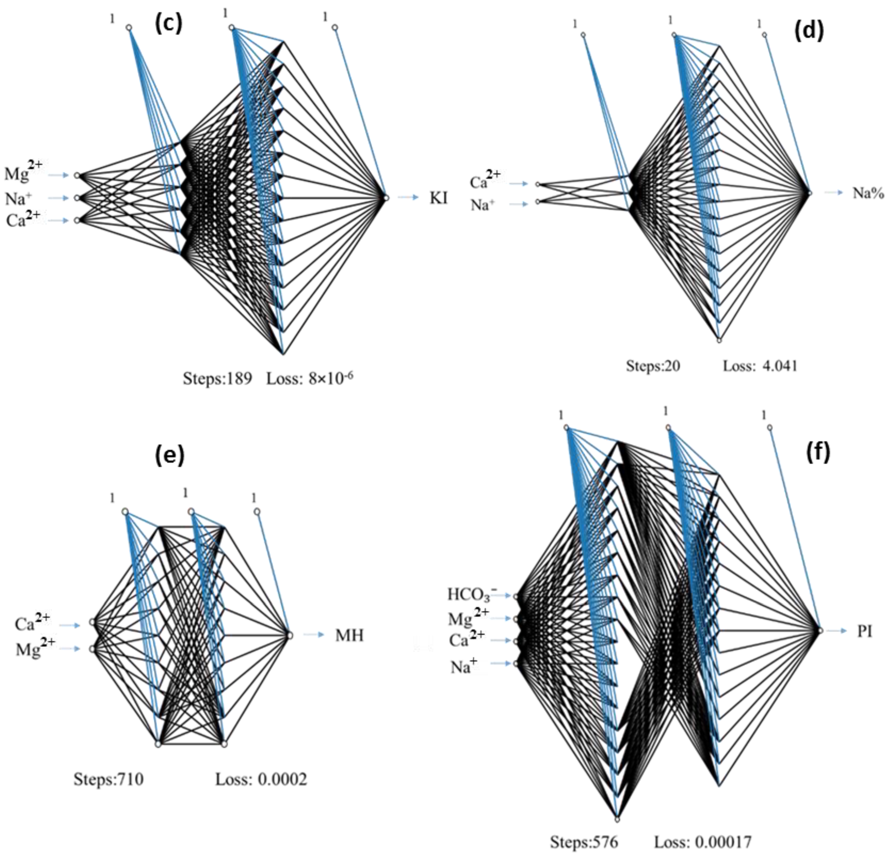
| ANN | Mg2⁺, Na+, Ca2⁺ | (h1 = 6, h2 = 15, fun = tanh) | 0.999 | 0.002 | 0.999 | 0.004 | |
| Na% | GBR | Mg2⁺, Ca2⁺, Na+ | (Ns = 25, Mf = auto) | 0.990 | 0.909 | 0.783 | 3.186 |
| ANN | Ca2⁺, Na+ | (h1 = 3, h2 = 18, fun = identity) | 1.0 | 2.306 × 10⁻⁷ | 1.0 | 4.169 × 10⁻⁷ | |
| MH | GBR | Ca2⁺, Mg2⁺ | (Ns = 25, Mf = auto) | 0.969 | 1.125 | 0.557 | 2.946 |
| ANN | Ca2⁺, Mg2⁺ | (h1 = 9, h2 = 9, fun = logistic) | 0.999 | 0.005 | 0.999 | 0.036 | |
| PI | GBR | Na+, Mg2⁺ | (Ns = 25, Mf = auto) | 0.984 | 1.093 | 0.577 | 4.147 |
| ANN | HCO₃⁻, Mg2⁺, Ca2⁺, Na+ | (h1 = 18, h2 = 15, fun = logistic) | 0.999 | 0.003 | 0.999 | 0.106 | |
Disclaimer/Publisher’s Note: The statements, opinions and data contained in all publications are solely those of the individual author(s) and contributor(s) and not of MDPI and/or the editor(s). MDPI and/or the editor(s) disclaim responsibility for any injury to people or property resulting from any ideas, methods, instructions or products referred to in the content. |
© 2023 by the authors. Licensee MDPI, Basel, Switzerland. This article is an open access article distributed under the terms and conditions of the Creative Commons Attribution (CC BY) license (https://creativecommons.org/licenses/by/4.0/).
Share and Cite
Gaagai, A.; Aouissi, H.A.; Bencedira, S.; Hinge, G.; Athamena, A.; Heddam, S.; Gad, M.; Elsherbiny, O.; Elsayed, S.; Eid, M.H.; et al. Application of Water Quality Indices, Machine Learning Approaches, and GIS to Identify Groundwater Quality for Irrigation Purposes: A Case Study of Sahara Aquifer, Doucen Plain, Algeria. Water 2023, 15, 289. https://doi.org/10.3390/w15020289
Gaagai A, Aouissi HA, Bencedira S, Hinge G, Athamena A, Heddam S, Gad M, Elsherbiny O, Elsayed S, Eid MH, et al. Application of Water Quality Indices, Machine Learning Approaches, and GIS to Identify Groundwater Quality for Irrigation Purposes: A Case Study of Sahara Aquifer, Doucen Plain, Algeria. Water. 2023; 15(2):289. https://doi.org/10.3390/w15020289
Chicago/Turabian StyleGaagai, Aissam, Hani Amir Aouissi, Selma Bencedira, Gilbert Hinge, Ali Athamena, Salim Heddam, Mohamed Gad, Osama Elsherbiny, Salah Elsayed, Mohamed Hamdy Eid, and et al. 2023. "Application of Water Quality Indices, Machine Learning Approaches, and GIS to Identify Groundwater Quality for Irrigation Purposes: A Case Study of Sahara Aquifer, Doucen Plain, Algeria" Water 15, no. 2: 289. https://doi.org/10.3390/w15020289