
Flocculation Patterns Related to Intra-Annual Hydrodynamics Variability in the Lower Grijalva-Usumacinta System
 , , and
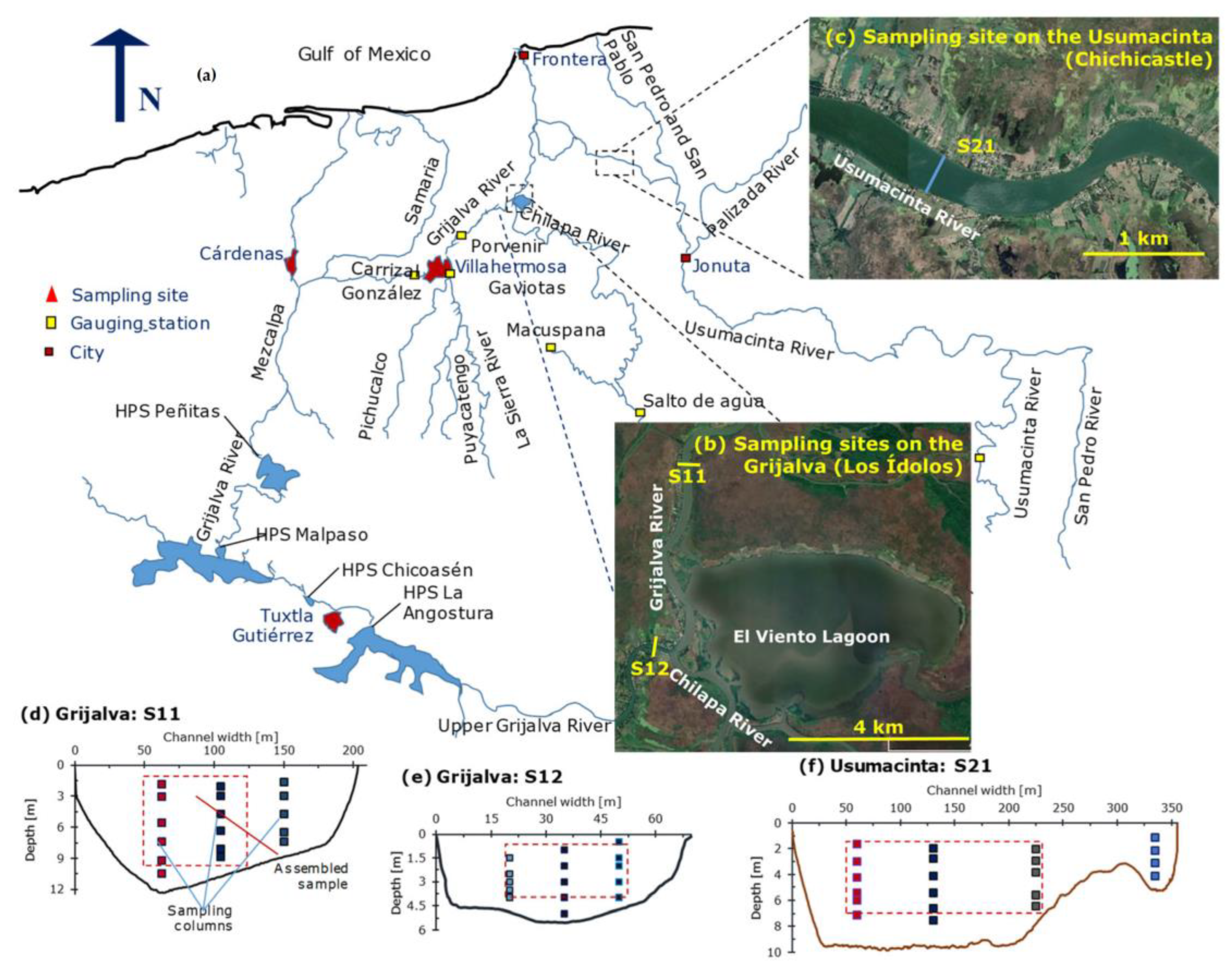
Abstract
:1. Introduction
2. Materials and Methods
2.1. Study Area
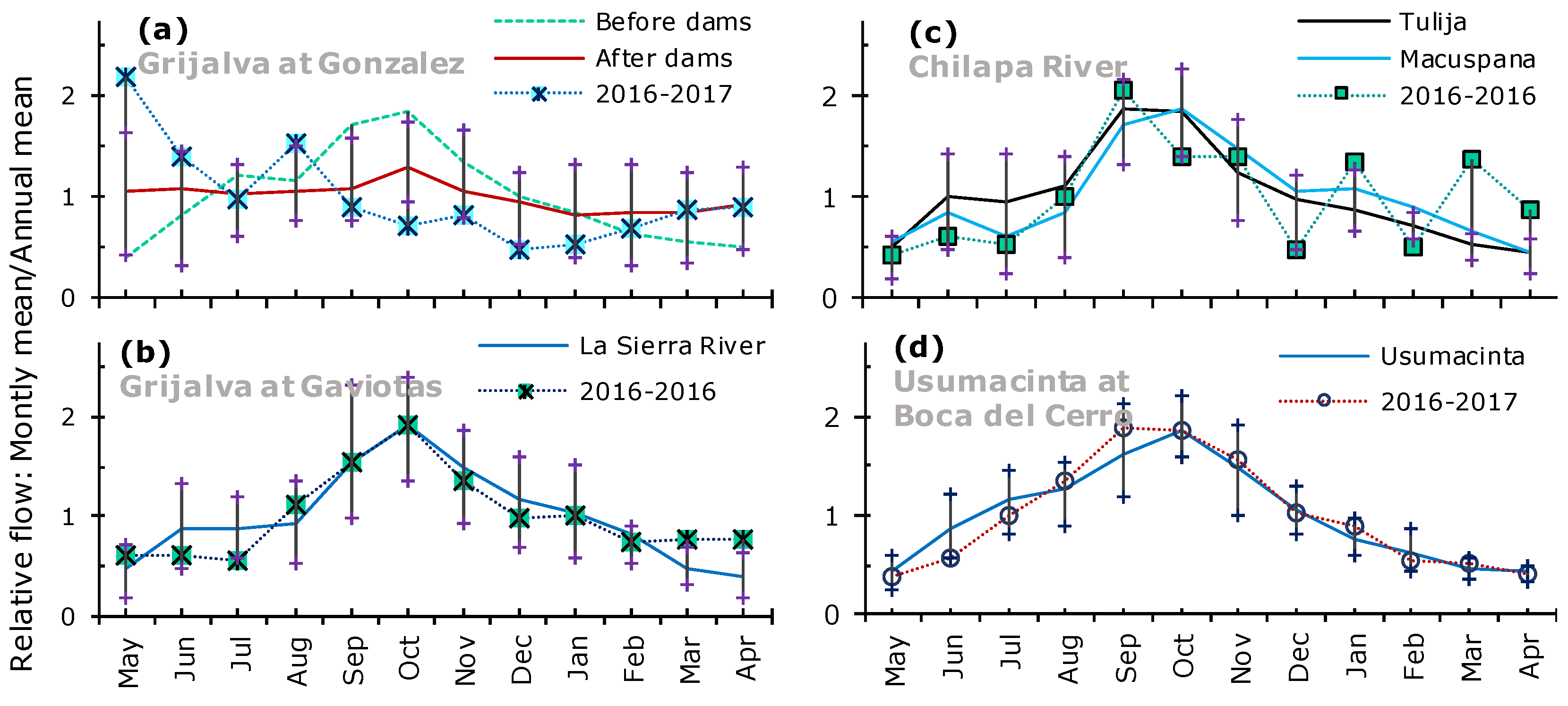
2.2. Montlhy and Seasonal River Data
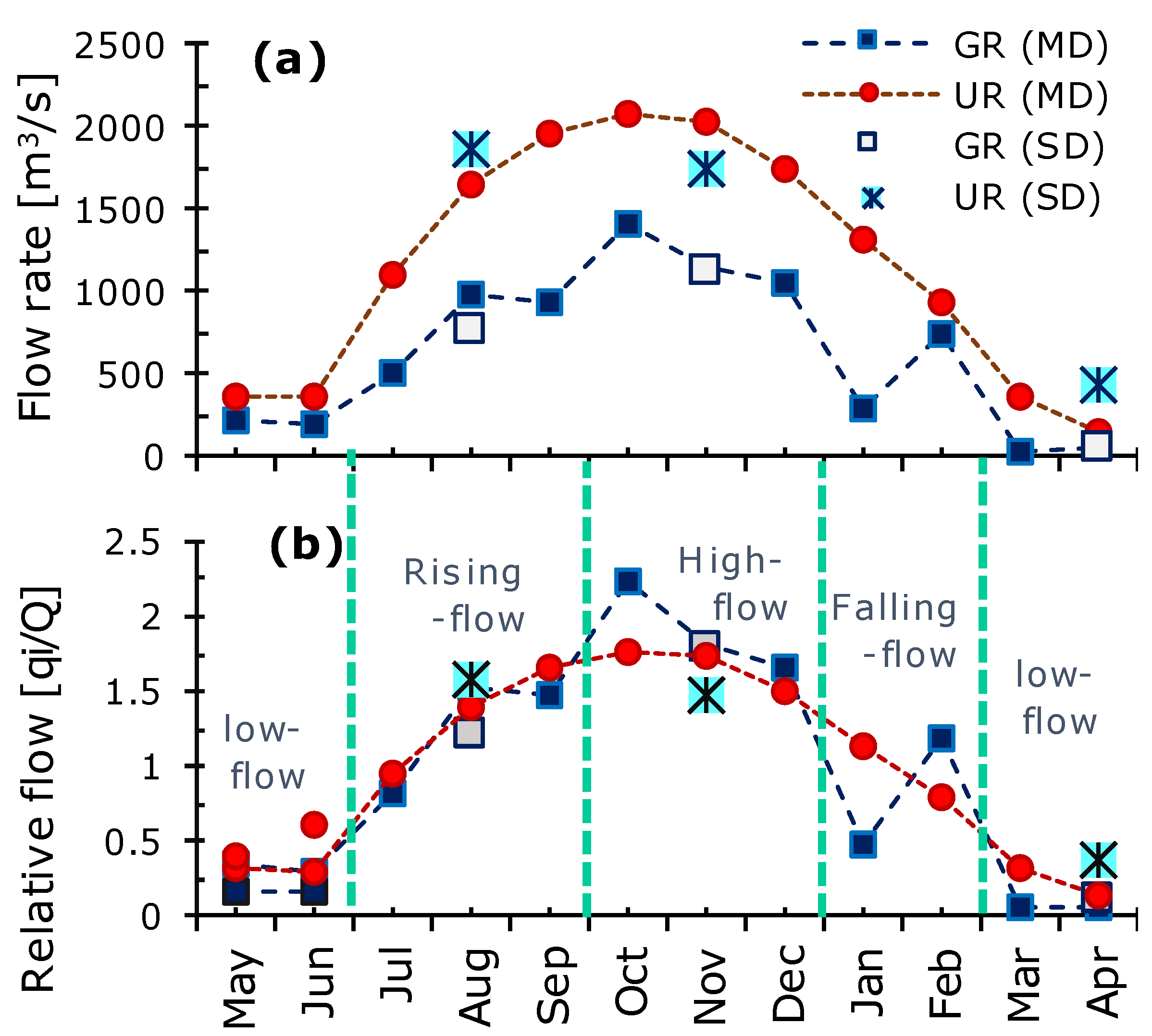
2.3. Hydrological Regimen
2.4. Floc Characterization
2.5. River Hydrodynamics
2.6. TSS Derived from Fluid Corrected Backscatter FCB
2.7. Effective Settling Velocity
2.8. Flocculation Intensity
3. Results
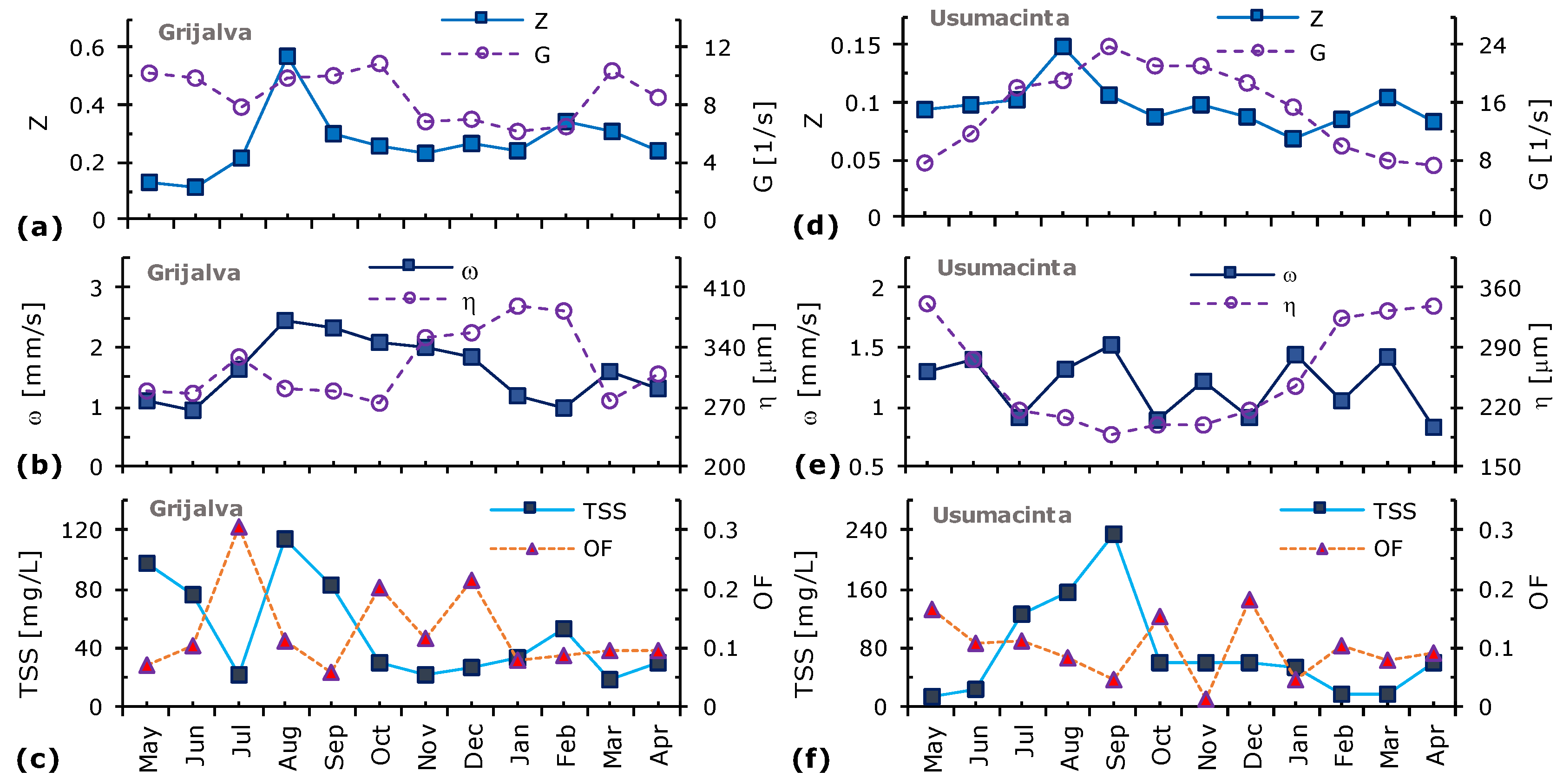
3.1. Intra-Annual Variability in Suspended Load
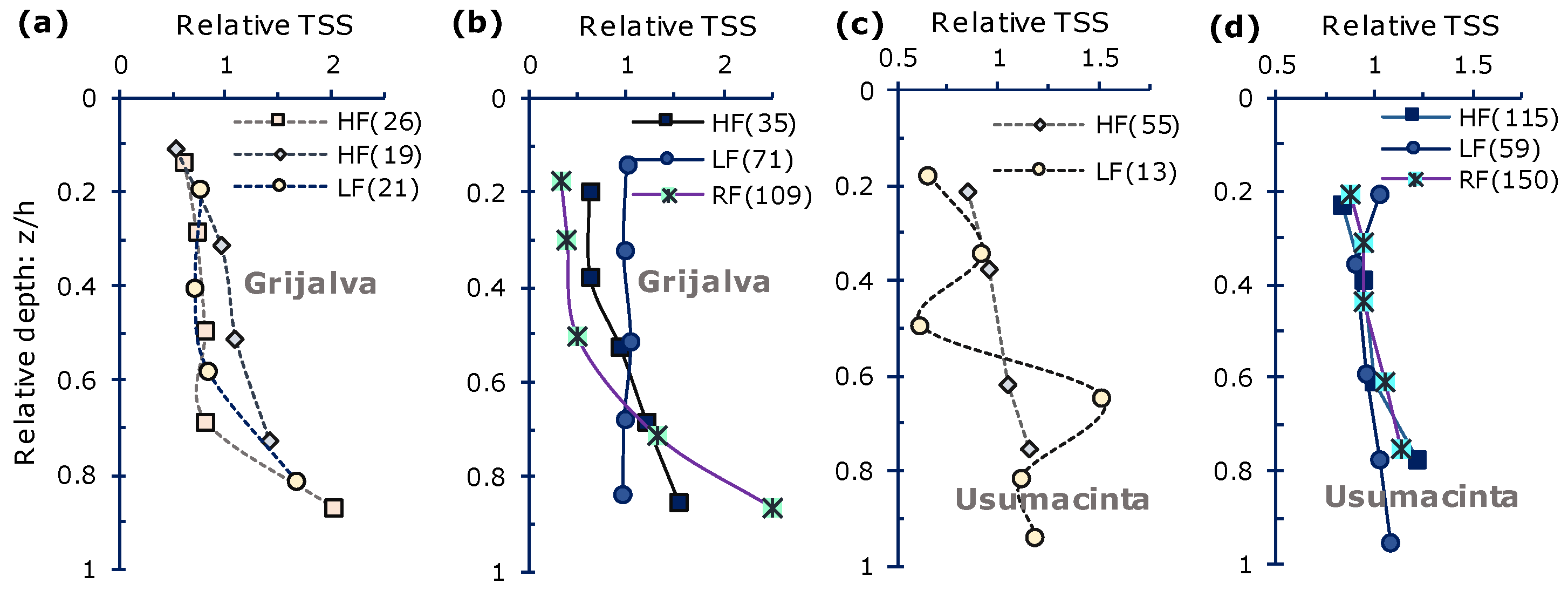
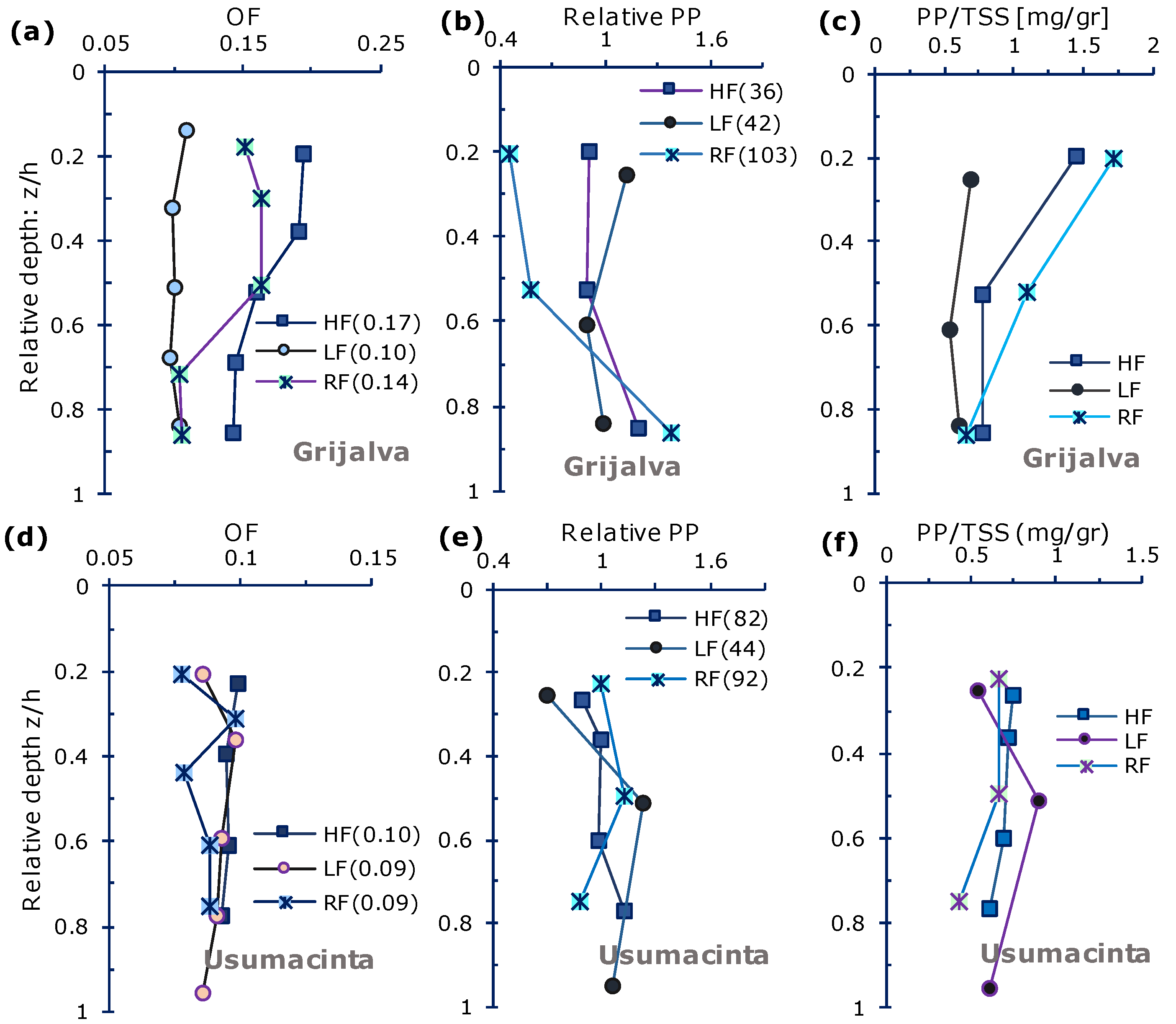
3.2. TSS, OF, and PP Profiles
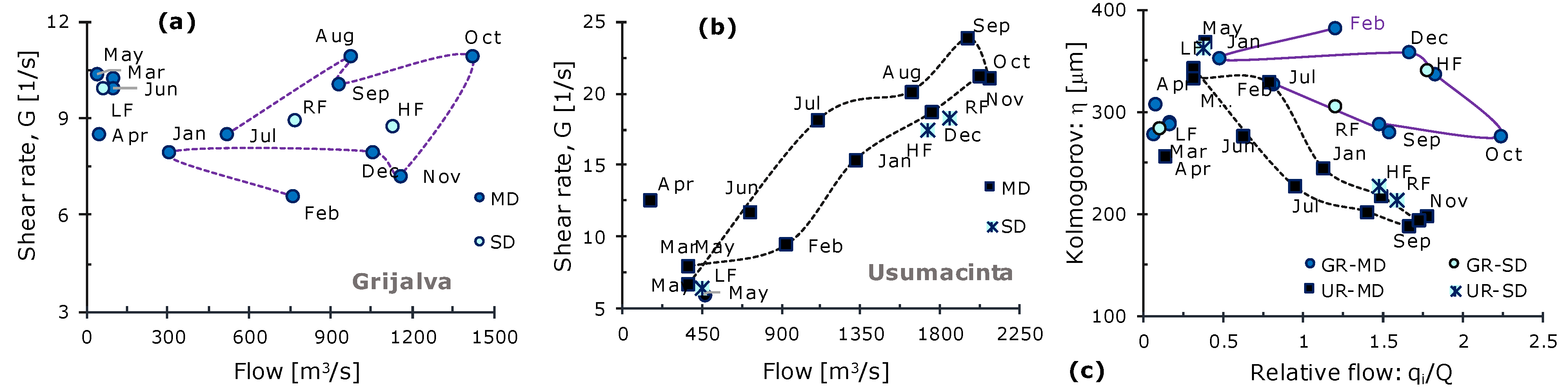
3.3. Hydrodynamic Forces
3.4. Flocculation Prevalence
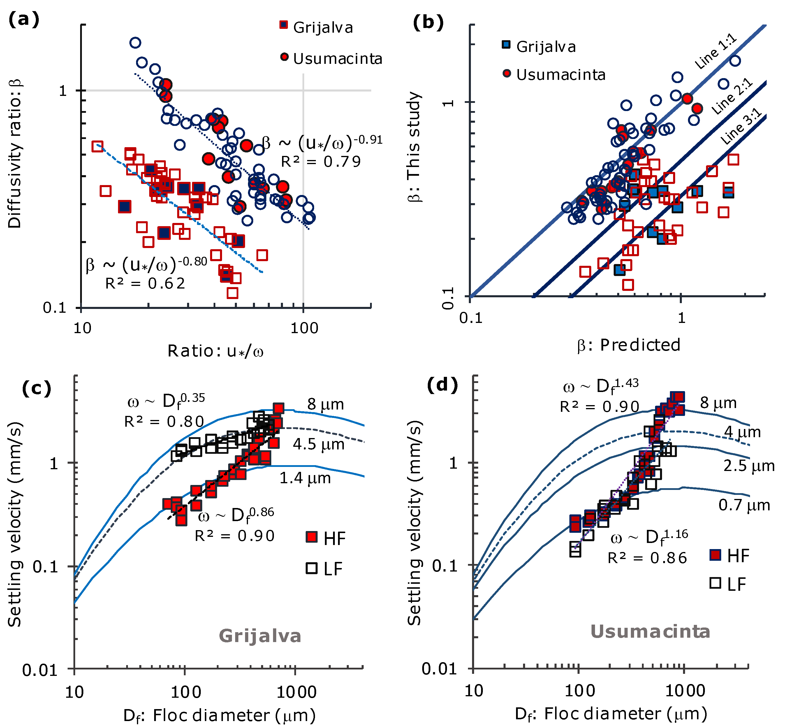
3.5. Diffusivity Ratio and Floc Size
4. Discussion
4.1. Study Findings
4.2. Seasonality and Flocculation Patterns
4.3. Flow Regulation
4.4. Implications on Particulate Nutrients on SSF
4.5. Limitations, Strenghts, and Pending Tasks
5. Conclusions
Author Contributions
Funding
Data Availability Statement
Acknowledgments
Conflicts of Interest
References
- Walsh, J.P.; Nittrouer, C.A. Understanding fine-grained river-sediment dispersal on continental margins. Mar. Geol. 2009, 263, 34–45. [Google Scholar] [CrossRef]
- Caldwell, R.L.; Edmonds, D.A. The effects of sediment properties on deltaic processes and morphologies: A numerical modeling study. J. Geophys. Res. Earth Surf. 2014, 119, 961–982. [Google Scholar] [CrossRef]
- Manh, N.V.; Dung, N.V.; Hung, N.N.; Merz, B.; Apel, H. Large-scale suspended sediment transport and sediment deposition in the Mekong Delta. Hydrol. Earth Syst. Sci. 2014, 18, 3033–3053. [Google Scholar] [CrossRef] [Green Version]
- Guo, L.; Zhang, J.Z.; Guéguen, C. Speciation and fluxes of nutrients (N, P, Si) from the upper Yukon River. Glob. Biogeochem. Cycles 2004, 18, GB1038. [Google Scholar] [CrossRef]
- Bouchez, J.; Galy, V.; Hilton, R.G.; Gaillardet, J.; Moreira-Turcq, P.; Pérez, M.A.; France-Lanord, C.; Maurice, L. Source, transport and fluxes of amazon river particulate organic carbon: Insights from river sediment depth-profiles. Geochim. Cosmochim. Acta 2014, 133, 280–298. [Google Scholar] [CrossRef]
- Almeida, R.M.; Tranvik, L.; LM Huszar, V.; Sobek, S.; Mendonça, R.; Barros, N.; Boemer, G.; Durval Arantes, J., Jr.; Roland, F. Phosphorus transport by the largest Amazon tributary (Madeira River, Brazil) and its sensitivity to precipitation and damming. Inland Waters 2015, 5, 275–282. [Google Scholar] [CrossRef] [Green Version]
- Cai, Y.; Guo, L.; Wang, X.; Aiken, G. Abundance, stable isotopic composition, and export fluxes of DOC, POC, and DIC from the Lower Mississippi River during 2006–2008. J. Geophys. Res. Biogeosciences 2015, 120, 2273–2288. [Google Scholar] [CrossRef] [Green Version]
- Yao, Q.Z.; Du, J.T.; Chen, H.T.; Yu, Z.G. Particle-size distribution and phosphorus forms as a function of hydrological forcing in the Yellow River. Environ. Sci. Pollut. Res. 2016, 23, 3385–3398. [Google Scholar] [CrossRef]
- Schindler, R.J.; Comber, S.D.W.; Manning, A.J. Metal pollutant pathways in cohesive coastal catchments: Influence of flocculation and biopolymers on partitioning and flux. Sci. Total Environ. 2021, 795, 148800. [Google Scholar] [CrossRef] [PubMed]
- Williams, N.; Walling, D.; Leeks, G. An analysis of the factors contributing to the settling potential of fine fluvial sediment. Hydrol. Process. Int. J. 2008, 22, 4153–4162. [Google Scholar] [CrossRef]
- Droppo, I.G.; D’Andrea, L.; Krishnappan, B.G.; Jaskot, C.; Trapp, B.; Basuvaraj, M.; Liss, S.N. Fine-sediment dynamics: Towards an improved understanding of sediment erosion and transport. J. Soils Sediments 2015, 15, 467–479. [Google Scholar] [CrossRef]
- Marttila, H.; Bjørn, K. Spatial and temporal variation in particle size and particulate organic matter content in suspended particulate matter from peatland-dominated catchments in Finland. Hydrol. Process. 2015, 29, 1069–1079. [Google Scholar] [CrossRef]
- Bouchez, J.; Métivier, F.; Lupker, M.; Maurice, L.; Perez, M.; Gaillardet, J.; France-Lanord, C. Prediction of depth-integrated fluxes of suspended sediment in the amazon river: Particle aggregation as a complicating factor. Hydrol. Process. 2011, 25, 778–794. [Google Scholar] [CrossRef]
- Guo, L.; He, Q. Freshwater flocculation of suspended sediments in the yangtze river, China. Ocean. Dyn. 2011, 61, 371–386. [Google Scholar] [CrossRef]
- Le, H.A.; Gratiot, N.; Santini, W.; Ribolzi, O.; Tran, D.; Meriaux, X.; Deleersnijder, E.; Soares-Frazão, S. Suspended sediment properties in the Lower Mekong River, from fluvial to estuarine environments. Estuar. Coast. Shelf Sci. 2020, 233, 106522. [Google Scholar] [CrossRef]
- Li, W.; Yu, C.; Yang, S.; Yang, Y.; Yang, W.; Xiao, Y. Measurements of the sediment flocculation characteristics in the Three Gorges Reservoir, Yangtze River. River Res. Appl. 2020, 36, 1202–1212. [Google Scholar] [CrossRef]
- Lamb, M.P.; de Leeuw, J.; Fischer, W.W.; Moodie, A.J.; Venditti, J.G.; Nittrouer, J.A.; Haught, D.; Parker, G. Mud in rivers transported as flocculated and suspended bed material. Nat. Geosci. 2020, 13, 566–570. [Google Scholar] [CrossRef]
- Coynel, A.; Seyler, P.; Etcheber, H.; Meybeck, M.; Orange, D. Spatial and seasonal dynamics of total suspended sediment and organic carbon species in the congo river. Glob. Biogeochem. Cycles 2005, 19, GB4019. [Google Scholar] [CrossRef]
- Picouet, C.; Hingray, B.; Olivry, J.C. Modelling the suspended sediment dynamics of a large tropical river: The Upper Niger River basin at Banankoro. Hydrol. Process. Int. J. 2009, 23, 3193–3200. [Google Scholar] [CrossRef]
- Malutta, S.; Kobiyama, M.; Chaffe, P.L.B.; Bonumá, N.B. Hysteresis analysis to quantify and qualify the sediment dynamics: State of the art. Water Sci. Technol. 2020, 81, 2471–2487. [Google Scholar] [CrossRef]
- Bainbridge, Z.T.; Lewis, S.E.; Smithers, S.G.; Kuhnert, P.M.; Henderson, B.L.; Brodie, J.E. Fine-suspended sediment and water budgets for a large, seasonally dry tropical catchment: Burdekin River catchment, Queensland, Australia. Water Resour. Res. 2014, 50, 9067–9087. [Google Scholar] [CrossRef] [Green Version]
- Lee, B.J.; Kim, J.; Hur, J.; Choi, I.H.; Toorman, E.A.; Fettweis, M.; Choi, J.W. Seasonal dynamics of organic matter composition and its effects on suspended sediment flocculation in river water. Water Resour. Res. 2019, 55, 6968–6985. [Google Scholar] [CrossRef]
- Livsey, D.N.; Crosswell, J.R.; Turner, R.D.R.; Steven, A.D.L.; Grace, P.R. Flocculation of Riverine Sediment Draining to the Great Barrier Reef, Implications for Monitoring and Modeling of Sediment Dispersal Across Continental Shelves. J. Geophys. Res. Oceans 2022, 127, e2021JC017988. [Google Scholar] [CrossRef]
- Mietta, F.; Chassagne, C.; Manning, A.J.; Winterwerp, J.C. Influence of shear rate, organicmatter content, ph and salinity onmud flocculation. Ocean Dyn. 2009, 59, 751–763. [Google Scholar] [CrossRef] [Green Version]
- Fettweis, M.; Schartau, M.; Desmit, X.; Lee, B.J.; Terseleer, N.; Van der Zande, D.; Parmentier, K.; Riethmüller, R. Organic matter composition of biomineral flocs and its influence on suspended particulate matter dynamics along a nearshore to offshore transect. J. Geophys. Res. Biogeosciences 2022, 127, e2021JG006332. [Google Scholar] [CrossRef]
- Fall, K.A.; Friedrichs, C.T.; Massey, G.M.; Bowers, D.G.; Smith, S.J. The importance of organic content to fractal floc properties in estuarine surface waters: Insights from video, LISST, and pump sampling. J. Geophys. Res. Oceans 2021, 126, e2020JC016787. [Google Scholar] [CrossRef]
- Spencer, K.L.; Wheatland, J.A.; Bushby, A.J.; Carr, S.J.; Droppo, I.G.; Manning, A.J. A structure–function based approach to floc hierarchy and evidence for the non-fractal nature of natural sediment flocs. Sci. Rep. 2021, 11, 1–10. [Google Scholar] [CrossRef]
- Biggs, B.J.; Nikora, V.I.; Snelder, T.H. Linking scales of flow variability to lotic ecosystem structure and function. River Res. Appl. 2005, 21, 283–298. [Google Scholar] [CrossRef]
- Nikora, V. Hydrodynamics of aquatic ecosystems: An interface between ecology, biomechanics and environmental fluid mechanics. River Res. Appl. 2010, 26, 367–384. [Google Scholar] [CrossRef]
- Zhou, J.; Zhang, M.; Lin, B.; Lu, P. Lowland fluvial phosphorus altered by dams. Water Resour. Res. 2015, 51, 2211–2226. [Google Scholar] [CrossRef]
- Wang, H.; Wu, X.; Bi, N.; Li, S.; Yuan, P.; Wang, A.; Syvitski, J.P.; Saito, Y.; Yang, Z.; Liu, S.; et al. Impacts of the dam-orientated water-sediment regulation scheme on the lower reaches and delta of the Yellow River (Huanghe): A review. Glob. Planet. Change 2017, 157, 93–113. [Google Scholar] [CrossRef]
- Maavara, T.; Chen, Q.; Van Meter, K.; Brown, L.E.; Zhang, J.; Ni, J.; Zarfl, C. River dam impacts on biogeochemical cycling. Nat. Rev. Earth Environ. 2020, 1, 103–116. [Google Scholar] [CrossRef] [Green Version]
- Owens, P.N.; Batalla, R.J.; Collins, A.J.; Gomez, B.; Hicks, D.M.; Horowitz, A.J.; Kondolf, G.M.; Marden, M.; Page, M.J.; Peacock, D.H.; et al. Fine-grained sediment in river systems: Environmental significance and management issues. River Res. Appl. 2005, 21, 693–717. [Google Scholar] [CrossRef]
- Nikora, V.I.; Goring, D.G. Fluctuations of suspended sediment concentration and turbulent sediment fluxes in an open-channel flow. J. Hydraul. Eng. 2002, 128, 214–224. [Google Scholar] [CrossRef]
- Manning, A.J.; Baugh, J.V.; Spearman, J.R.; Whitehouse, R.J. Flocculation settling characteristics of mud: Sand mixtures. Ocean Dyn. 2010, 60, 237–253. [Google Scholar] [CrossRef]
- Lupker, M.; France-Lanord, C.; Lavé, J.; Bouchez, J.; Galy, V.; Métivier, F.; Gaillardet, J.; Lartiges, B.; Mugnier, J.-L. A rouse-based method to integrate the chemical composition of river sediments: Application to the Ganga basin. J. Geophys. Res. Earth Surf. 2011, 116, F4012. [Google Scholar] [CrossRef] [Green Version]
- Venditti, J.G.; Church, M.; Attard, M.E.; Haught, D. Use of ADCPs for suspended sediment transport monitoring: An empirical approach. Water Resour. Res. 2016, 52, 2715–2736. [Google Scholar] [CrossRef]
- Salinas-Rodríguez, S.A.; Barba-Macías, E.; Infante Mata, D.; Nava-López, M.Z.; Neri-Flores, I.; Domínguez Varela, R.; González Mora, I.D. What Do Environmental Flows Mean for Long-term Freshwater Ecosystems’ Protection? Assessment of the Mexican Water Reserves for the Environment Program. Sustainability 2021, 13, 1240. [Google Scholar] [CrossRef]
- Yánez-Arancibia, A.; Day, J.W.; Currie-Alder, B. Functioning of the Grijalva-Usumacinta river delta, Mexico: Challenges for coastal management. Ocean Yearb. Online 2009, 23, 473–501. [Google Scholar] [CrossRef]
- Yáñez-Arancibia, A.; Lara-Domínguez, A.L.; Sánchez-Gil, P.; Day, J.W. Estuary-sea ecological interactions: A theoretical framework for the management of coastal environment. In Environmental Analysis of the Gulf of Mexico; Harte Research Institute for Gulf of Mexico Studies: Corpus Christi, TX, USA, 2007; pp. 271–301. [Google Scholar]
- Arreguín-Cortés, F.I.; Rubio-Gutiérrez, H.; Domínguez-Mora, R.; Luna-Cruz, F.d. Análisis de las inundaciones en la planicie tabasqueña en el periodo 1995–2010. Tecnol. Cienc. Agua 2014, 5, 5–32. [Google Scholar]
- Horton, A.J.; Nygren, A.; Diaz-Perera, M.A.; Kummu, M. Flood severity along the usumacinta river, mexico: Identifying the anthropogenic signature of tropical forest conversion. J. Hydrol. X 2021, 10, 100072. [Google Scholar] [CrossRef]
- Lotsari, E.; Aaltonen, J.; Veijalainen, N.; Alho, P.; Käyhkö, J. Future fluvial erosion and sedimentation potential of cohesive sediments in a coastal river reach of SW Finland. Hydrol. Process. 2014, 28, 6016–6037. [Google Scholar] [CrossRef]
- APHA; AWWA; WPCF; Greenberg, W.I.A.; Clesceri, L.; Eaton, A. Standard Methods for the Examination of Water Andwastewater; American Public Health Association: Wasghington, DC, USA, 2012. [Google Scholar]
- Nooren, K.; Hoek, W.Z.; Winkels, T.; Huizinga, A.; Van der Plicht, H.; Van Dam, R.L.; Van Heteren, S.; Van Bergen, M.J.; Prins, M.A.; Reimann, T.; et al. The Usumacinta-Grijalva beach-ridge plain in southern Mexico: A high-resolution archive of river discharge and precipitation. Earth Surf. Dyn. 2017, 5, 529–556. [Google Scholar] [CrossRef] [Green Version]
- Munoz-Salinas, E.; Castillo, M. Streamflow and sediment load assessment from 1950 to 2006 in the usumacinta and grijalva rivers (southern mexico) and the influence of enso. Catena 2015, 127, 270–278. [Google Scholar] [CrossRef]
- Vaca, R.A.; Golicher, D.J.; Rodiles-Hernández, R.; Castillo-Santiago, M.Á.; Bejarano, M.; Navarrete-Gutiérrez, D.A. Drivers of deforestation in the basin of the usumacinta river: Inference on process from pattern analysis using generalised additive models. PLoS ONE 2009, 14, e0222908. [Google Scholar]
- Lázaro-Vázquez, A.; Castillo, M.; Jarquín-Sánchez, A.; Carrillo, L.; Capps, K. Temporal changes in the hydrology and nutrient concentrations of a large tropical river: Anthropogenic influence in the lower grijalva river, mexico. River Res. Appl. 2018, 34, 649–660. [Google Scholar] [CrossRef]
- Castillo, M.M. Suspended sediment, nutrients, and chlorophyll in tropical floodplain lakes with different patterns of hydrological connectivity. Limnologica 2020, 82, 125767. [Google Scholar] [CrossRef]
- Cuevas-Lara, D.; Alcocer, J.; Cortés-Guzmán, D.; Soria-Reinoso, I.F.; García-Oliva, F.; Sánchez-Carrillo, S.; Oseguera, L.A. Particulate organic carbon in the tropical usumacinta river, southeast mexico: Concentration, flux, and sources. Water 2021, 13, 1561. [Google Scholar] [CrossRef]
- Cardoso-Mohedano, J.G.; Canales-Delgadillo, J.C.; Machain-Castillo, M.L.; Sanchez-Muñoz, W.N.; Sanchez-Cabeza, J.A.; Esqueda-Lara, K.; Gómez-Ponce, M.A.; Ruiz-Fernández, A.C.; Alonso-Rodríguez, R.; Lestayo-González, J.A.; et al. Contrasting nutrient distributions during dry and rainy seasons in coastal waters of the southern Gulf of Mexico driven by the Grijalva-Usumacinta River discharges. Mar. Pollut. Bull. 2022, 178, 113584. [Google Scholar] [CrossRef]
- Alcérreca-Huerta, J.; Callejas-Jiménez, M.; Carrillo, L.; Castillo, M. Dam implications on salt-water intrusion and land use within a tropical estuarine environment of the gulf of mexico. Sci. Total Environ. 2019, 652, 1102–1112. [Google Scholar] [CrossRef] [PubMed]
- Mendoza, A.; Soto-Cortes, G.; Priego-Hernandez, G.; Rivera-Trejo, F. Historical description of the morphology and hydraulic behavior of a bifurcation in the lowlands of the Grijalva River Basin, Mexico. Catena 2019, 176, 343–351. [Google Scholar] [CrossRef]
- Winterwerp, J.; Manning, A.; Martens, C.; de Mulder, T.; Vanlede, J. A heuristic formula for turbulence-induced flocculation of cohesive sediment. Estuar. Coast. Shelf Sci. 2006, 68, 195–207. [Google Scholar] [CrossRef]
- Soulsby, R.; Manning, A.; Spearman, J.; Whitehouse, R. Settling velocity and mass settling flux of flocculated estuarine sediments. Mar. Geol. 2013, 339, 1–12. [Google Scholar] [CrossRef] [Green Version]
- Garcia-Aragon, J.; Salinas-Tapia, H.; Moreno-Guevara, J.; Diaz-Palomarez, V.; Tejeda-Vega, S. A model for the settling velocity of flocs; application to an aquaculture recirculation tank. Int. J. Comput. Methods Exp. Meas. 2014, 2, 313–322. [Google Scholar] [CrossRef] [Green Version]
- Félix-Félix, J.R.; Salinas-Tapia, H.; Bautista-Capetillo, C.; Garcia-Aragon, J.; Burguete, J.; Playan, E. A modified particle tracking velocimetry technique to characterize sprinkler irrigation drops. Irrig. Sci. 2017, 35, 515–531. [Google Scholar] [CrossRef]
- Sukhodolov, A.N.; Fedele, J.J.; Rhoads, B.L. Structure of flow over alluvial bedforms: An experiment on linking field and laboratory methods. Earth Surf. Process. Landf. 2006, 31, 1292–1310. [Google Scholar] [CrossRef]
- Fugate, D.C.; Friedrichs, C.T. Controls on suspended aggregate size in partially mixed estuaries. Estuar. Coast. Shelf Sci. 2003, 58, 389–404. [Google Scholar] [CrossRef]
- Afzalimehr, H.; Rennie, C.D. Determination of bed shear stress in gravel-bed rivers using boundary-layer parameters. Hydrol. Sci. J. 2009, 54, 147–159. [Google Scholar] [CrossRef] [Green Version]
- Bagherimiyab, F.; Lemmin, U. Shear velocity estimates in rough-bed open-channel flow. Earth Surf. Process. Landf. 2013, 38, 1714–1724. [Google Scholar] [CrossRef] [Green Version]
- Baronas, J.J.; Stevenson, E.I.; Hackney, C.R.; Darby, S.E.; Bickle, M.J.; Hilton, R.G.; Larkin, C.S.; Parsons, D.R.; Myo Khaing, A.; Tipper, E.T. Integrating suspended sediment flux in large alluvial river channels: Application of a synoptic rouse-based model to the irrawaddy and salween rivers. J. Geophys. Res. Earth Surf. 2020, 125, e2020JF005554. [Google Scholar] [CrossRef]
- Castro-Orgaz, O.; Giráldez, J.V.; Mateos, L.; Dey, S. Is the von Kármán constant affected by sediment suspension? J. Geophys. Res. Earth Surf. 2012, 117, F4002. [Google Scholar] [CrossRef] [Green Version]
- Ha, H.K.; Maa, J.P.-Y. Effects of suspended sediment concentration and turbulence on settling velocity of cohesive sediment. Geosci. J. 2010, 14, 163–171. [Google Scholar] [CrossRef]
- Strom, K.; Keyvani, A. Flocculation in a decaying shear field and its implications for mud removal in near-field river mouth discharges. J. Geophys. Res. Ocean. 2016, 121, 2142–2162. [Google Scholar] [CrossRef]
- Kuprenas, R.; Tran, D.; Strom, K. A shear-limited flocculation model for dynamically predicting average floc size. J. Geophys. Res. Ocean. 2018, 123, 6736–6752. [Google Scholar] [CrossRef]
- Nghiem, J.A.; Fischer, W.W.; Li, G.K.; Lamb, M.P. A Mechanistic Model for Mud Flocculation in Freshwater Rivers. J. Geophys. Res. Earth Surf. 2022, 127, e2021JF006392. [Google Scholar] [CrossRef]
- Guo, C.; He, Q.; van Prooijen, B.C.; Guo, L.; Manning, A.J.; Bass, S. Investigation of flocculation dynamics under changing hydrodynamic forcing on an intertidal mudflat. Mar. Geol. 2018, 395, 120–132. [Google Scholar] [CrossRef]
- Latosinski, F.G.; Szupiany, R.N.; García, C.M.; Guerrero, M.; Amsler, M.L. Estimation of concentration and load of suspended bed sediment in a large river by means of acoustic Doppler technology. J. Hydraul. Eng. 2014, 140, 04014023. [Google Scholar] [CrossRef]
- Guerrero, M.; Rüther, N.; Szupiany, R.; Haun, S.; Baranya, S.; Latosinski, F. The acoustic properties of suspended sediment in large rivers: Consequences on ADCP methods applicability. Water 2016, 8, 13. [Google Scholar] [CrossRef] [Green Version]
- Baranya, S.; Józsa, J. Estimation of suspended sediment concentrations with ADCP in Danube River. J. Hydrol. Hydromech. 2013, 61, 232. [Google Scholar] [CrossRef] [Green Version]
- Wosiacki, L.F.; Suekame, H.K.; Wood, M.S.; Gonçalves, F.V.; Bleninger, T. Mapping of suspended sediment transport using acoustic methods in a Pantanal tributary. Environ. Monit. Assess. 2021, 193, 1–19. [Google Scholar] [CrossRef]
- Chalov, S.; Moreido, V.; Ivanov, V.; Chalova, A. Assessing suspended sediment fluxes with acoustic Doppler current profilers: Case study from large rivers in Russia. Big Earth Data 2022, 6, 504–526. [Google Scholar] [CrossRef]
- Sahin, C.; Safak, I.; Hsu, T.J.; Sheremet, A. Observations of suspended sediment stratification from acoustic backscatter in muddy environments. Mar. Geol. 2013, 336, 24–32. [Google Scholar] [CrossRef]
- Sahin, C.; Verney, R.; Sheremet, A.; Voulgaris, G. Acoustic backscatter by suspended cohesive sediments: Field observations, Seine Estuary, France. Cont. Shelf Res. 2017, 134, 39–51. [Google Scholar] [CrossRef] [Green Version]
- Maa, J.-Y.; Kwon, J.-I. Using adv for cohesive sediment settling velocity measurements. Estuar. Coast. Shelf Sci. 2007, 73, 351–354. [Google Scholar] [CrossRef]
- Cartwright, G.M.; Friedrichs, C.T.; Smith, S.J. A test of the adv-based Reynolds flux method for in situ estimation of sediment settling velocity in a muddy estuary. Geo-Mar. Lett. 2013, 33, 477–484. [Google Scholar] [CrossRef]
- Bombardelli, F.A.; Jha, S.K. Hierarchical modeling of the dilute transport of suspended sediment in open channels. Environ. Fluid Mech. 2009, 9, 207–235. [Google Scholar] [CrossRef]
- Khelifa, A.; Hill, P.S. Models for effective density and settling velocity of flocs. J. Hydraul. Res. 2006, 44, 390–401. [Google Scholar] [CrossRef]
- Curran, K.; Hill, P.; Milligan, T.; Mikkelsen, O.; Law, B.; de Madron, X.D.; Bourrin, F. Settling velocity, effective density, and mass composition of suspended sediment in a coastal bottom boundary layer, Gulf of Lions, France. Cont. Shelf Res. 2007, 27, 1408–1421. [Google Scholar] [CrossRef]
- Smith, S.J.; Friedrichs, C.T. Size and settling velocities of cohesive flocs and suspended sediment aggregates in a trailing suction hopper dredge plume. Cont. Shelf Res. 2011, 31, S50–S63. [Google Scholar] [CrossRef]
- Rouse, H. Modern conceptions of the mechanics of fluid turbulence. Trans. Am. Soc. Civ. Eng. 1937, 102, 463–505. [Google Scholar] [CrossRef]
- Vanoni, V.A. Transportation of suspended sediment by water. Trans. Am. Soc. Civ. Eng. 1946, 111, 67–102. [Google Scholar] [CrossRef]
- De Leeuw, J.; Lamb, M.P.; Parker, G.; Moodie, A.J.; Haught, D.; Venditti, J.G.; Nittrouer, J.A. Entrainment and suspension of sand and gravel. Earth Surf. Dyn. 2020, 8, 485–504. [Google Scholar] [CrossRef]
- Liu, J.; Shen, Y.; Wang, X. Flocculation properties of cohesive fine-grained sediment in the Three Gorges Reservoir under variable turbulent shear. J. Mt. Sci. 2022, 19, 2286–2296. [Google Scholar] [CrossRef]
- Best, J. Anthropogenic stresses on the world’s big rivers. Nat. Geosci. 2019, 12, 7–21. [Google Scholar] [CrossRef]
- Jia, D.-D.; Shao, X.-J.; Zhang, X.-N.; Ye, Y.-T. Sedimentation patterns of fine-grained particles in the dam area of the Three Gorges Project: 3D numerical simulation. J. Hydraul. Eng. 2013, 139, 669–674. [Google Scholar] [CrossRef]
- Li, W.; Wang, J.; Yang, S.; Zhang, P. Determining the existence of the fine sediment flocculation in the Three Gorges Reservoir. J. Hydraul. Eng. 2015, 141, 05014008. [Google Scholar] [CrossRef]
- Bainbridge, Z.T.; Wolanski, E.; Álvarez-Romero, J.G.; Lewis, S.E.; Brodie, J.E. Fine sediment and nutrient dynamics related to particle size and floc formation in a Burdekin River flood plume, Australia. Mar. Pollut. Bull. 2012, 65, 236–248. [Google Scholar] [CrossRef]
- Garcia, C.M.; Oberg, K.; García, M.H. ADCP measurements of gravity currents in the Chicago River, Illinois. J. Hydraul. Eng. 2007, 133, 1356–1366. [Google Scholar] [CrossRef]
- Graham, G.W.; Nimmo Smith, W.A. The application of holography to the analysis of size and settling velocity of suspended cohesive sediments. Limnol. Oceanogr. Methods 2010, 8, 1–15. [Google Scholar] [CrossRef]


Disclaimer/Publisher’s Note: The statements, opinions and data contained in all publications are solely those of the individual author(s) and contributor(s) and not of MDPI and/or the editor(s). MDPI and/or the editor(s) disclaim responsibility for any injury to people or property resulting from any ideas, methods, instructions or products referred to in the content. |
© 2023 by the authors. Licensee MDPI, Basel, Switzerland. This article is an open access article distributed under the terms and conditions of the Creative Commons Attribution (CC BY) license (https://creativecommons.org/licenses/by/4.0/).
Share and Cite
Izquierdo-Ayala, K.; García-Aragón, J.A.; Castillo-Uzcanga, M.M.; Díaz-Delgado, C.; Carrillo, L.; Salinas-Tapia, H. Flocculation Patterns Related to Intra-Annual Hydrodynamics Variability in the Lower Grijalva-Usumacinta System. Water 2023, 15, 292. https://doi.org/10.3390/w15020292
Izquierdo-Ayala K, García-Aragón JA, Castillo-Uzcanga MM, Díaz-Delgado C, Carrillo L, Salinas-Tapia H. Flocculation Patterns Related to Intra-Annual Hydrodynamics Variability in the Lower Grijalva-Usumacinta System. Water. 2023; 15(2):292. https://doi.org/10.3390/w15020292
Chicago/Turabian StyleIzquierdo-Ayala, Klever, Juan Antonio García-Aragón, Maria Mercedes Castillo-Uzcanga, Carlos Díaz-Delgado, Laura Carrillo, and Humberto Salinas-Tapia. 2023. "Flocculation Patterns Related to Intra-Annual Hydrodynamics Variability in the Lower Grijalva-Usumacinta System" Water 15, no. 2: 292. https://doi.org/10.3390/w15020292