
Application of a Regionalization Method for Estimating Flash Floods: Cuautepec Basin, Mexico
by
Maritza Arganis
1,*,
Margarita Preciado
2,
Faustino De Luna
1,
Liliana Cruz
3,
Ramón Domínguez
1 and
Olaf Santana
1 1
Instituto de Ingeniería, Universidad Nacional Autónoma de México, Mexico City 04510, Mexico
2
Instituto Mexicano de Tecnología del Agua, Jiutepec 62550, Mexico
3
Comisión Nacional del Agua, Mexico City 04340, Mexico
*
Author to whom correspondence should be addressed.
Water 2023, 15(2), 303; https://doi.org/10.3390/w15020303
Submission received: 14 November 2022
/
Revised: 2 January 2023
/
Accepted: 4 January 2023
/
Published: 11 January 2023
(This article belongs to the Special Issue Flash Floods: Forecasting, Monitoring and Mitigation Strategies)
Abstract
:A rainfall regionalization method based on variation coefficient was applied with a variant in the construction of flash flood hyetographs with several return periods using the flash flood shape of the historical event that occurred in September 2021 in the Tlalnepantla River basin, Mexico, that caused severe damage to population and its infrastructure in a few hours. The historical flash flood was simulated with a semi-distributed model in the free software HEC-HMS in order to obtain the outflow hydrograph, and the flood plains were obtained with Iber and Hec-Ras 2d software that simulate free surface flow with a two-dimensional analysis. With photographs of the site, it was possible to locate traces of water that were contrasted with they calculated depths; they were concordant. Synthetic design storms were then simulated to estimate their potential consequences on the site.
1. Introduction
According to the National Weather Service [1], a flash flood is defined as runoff that occurs after the first 3 to 6 h after a heavy rain or some other cause. On the other hand, catastrophic floods are associated both with the intensity of the event and with the magnitude of the material damage they cause [2].
Flash floods have been the subject of studies going back nearly 25 years or more. Year after year they rise again, for example, in the face of different world events that have taken place over time; additionally, they appear in the recurrence of catastrophic floods.
At the global level, flash floods have been a study object for several decades; for example, Garzón et al. [3] make a description of morphology that occurs in terrain and natural channels before torrential floods occur, reporting some case studies highlighting ravines and river fans of basins in Spain (highlighting the Abanico of Arás where a terrible catastrophe occurred in 1996). They emphasize that the sense of security some flood protection works give must be distrusted, since they can be susceptible to failure in a flash flood event.
Aroca [4] analyzed the importance of characterizing initial abstraction prior to the runoff process associated with flash floods. Using the Green Amp method [5,6], comparing it with the curve number, generating the hydrograph with the SCS method [7], and using a semi-distributed hydrological model to simulate using Hec-Hms 4.0 software, he concluded in his study that the Green Amp method is better than the curve number method because it uses basin parameters, while the curve number method is reported as a method that is still empirical and was originally developed for basins of a specific country.
Karbasi et al. [8] developed a regional model for estimating loss of life due to flash flood in residential areas in the Kan watershed, Iran. They applied a model based on hydraulic variables such as depth, velocity, and rise rate of the water, as well as evacuation parameters, including available time for evacuation and fraction of people evacuated. They concluded that the most significant factors affecting fatalities, number of, were evacuation parameters, including evacuation time and fraction of evacuated people. From a local sensitivity analysis, the lead time between observed flood at the early flood warning station and the arrival time at the area of interest were distinguished as the most important input for evaluating the number of fatalities.
Aristizábal et al. [9] present a quantification of torrential floods and the population affected by torrential floods in various places in Colombia; they carried out torrential flood classification in terms of flash floods, debris flow, and debris flooding, reporting the last item as that with the greatest capacity for destruction. Due to the fact that there is no unanimity on the definition of torrential floods, the authors concluded that it is difficult to propose a methodology for threat assessment.
Bilasco et al. [10] present a methodology for the strategic management of floods to mitigate their damage in areas that anthropogenic activity has been invading for food production purposes; the analysis was carried out in the context of governance in the digital age. Their approach consists of a system that includes analysis and flooding, modeling, risk assessment, and diffusion of flood effects to the population.
Shuvo et al. [11] analyzed two flash floods due to monsoon events in Bangladesh using a coupled atmospheric–hydrological numerical weather prediction (NWP) model, namely the weather research and forecasting (WRF) model. Evaluating the goodness of the results with the mean square error and the Nash–Sutcliffe criterion, they found that the NWP model is applicable for flash flood prediction in the basins analyzed, despite the short duration of such events.
When making reviews and effect reconstructions caused by flash floods or making new simulations of events associated with a return period, the hyetograph shaping problem design has its particularities [12,13], since the traditional method of alternating blocks does not lead to the typical shape for storms associated with flash floods.
In this paper, a rainfall regionalization method was successfully applied [14] to obtain a design of flash floods associated with different return periods, but little variation in the hydrograph shape was obtained based on an ordering that takes into account the case of a historical event that occurred in the Tlalnepantla River basin in Mexico State (that is, the traditional alternating block method was not applied). These designed flash floods were simulated in a semi-distributed model using the HEC-HMS software [15], obtaining depth and velocity maps with the Iber software and Hec Ras 2d; additionally, the simulation for the historical flash flood was made to compare the results, in addition to contrasting them with photographic evidence of the water mark level.
The work is organized in the following parts: the introduction presented here, the methodology in which the procedures used and data from the study site are described, and the results and discussion, in addition to the conclusions derived from the research.
2. Methodology
2.1. Rainfall Regionalization Method Based on Variation Coefficient
This regionalization method [14] groups climatological stations that have daily precipitation historical data with more than 20 measurement years, based on the stations–year technique and variation coefficient (Equation (1)) for maximum precipitation series grouped in intervals after annual data sorting.
where
is the coefficient of variation of the maximum annual rainfall series;
is the standard deviation of the maximum annual rainfall series;
is the mean of the maximum annual rainfall series.
The first step is to identify the set of stations after the quality and quantity of information is checked. Then, the stations–year technique is applied, that is, each station was modulated or normalized with respect to its historical average and a large record was built by placing one normalized station after another. Later, an analysis of frequencies to find the regional distribution function of best fit was performed, with the least standard error criterion of fit (EEA) being between the measured data x and the calculated with a distribution function with p parameters, in an annual series of size n [14] given by the Equation (2).
With the regional distribution function obtained, regional factors associated with different return periods are obtained.
2.2. Estimation of the Design Storm from Regional Factors
To obtain a design storm associated with a return period, the following steps are used [14].
- The historical average maximum annual rainfall of the basin is estimated from an isohyet map and the approximate location of the basin centroid.
- The regional factor for the study site corresponding to the analyzed return period is selected.
- The historical average maximum annual rainfall is multiplied by the regional factor, thus obtaining the total annual maximum accumulated rainfall of 24 h.
- Rainfall previously obtained is affected by a reduction factor per area obtained with the basin area and the equation that corresponds to the study area.
- One-hour total rainfall is estimated from twenty-four-hour total rainfall data, calculated in step 4 with the help of the convective factor corresponding to the analysis site.
- Chen and Bell tables [16] are used to estimate precipitation values for durations between 1 and 24 h or for durations less than one hour or greater than 24 h.
- The design mass curve for the selected Δt is presented. The bars of the design hyetograph, not yet sorted, are defined for the duration of the selected storm.
- To shape the design storm, a block ordering process is carried out (alternating blocks are traditionally used in statistical storms, but in the case of flash floods, a skewness in the hyetograph must be considered).
2.3. Construction of the Design Hyetograph Using Flash Flood Shape
The variant proposed in this research occurs in the way of placing the design bars of the hyetograph associated with a flash flood.
For this, the historical storm event of the study site that caused a flash flood was selected and its position occupied by bars of the hyetograph was identified, from the largest to the smallest. This order was used to order the statistically generated storm bars; with the above, it is possible to obtain non-centered hyetographs with a skewness that correspond to a behavior similar to the hyetographs of a flash flood.
2.4. Study Site and Data Set
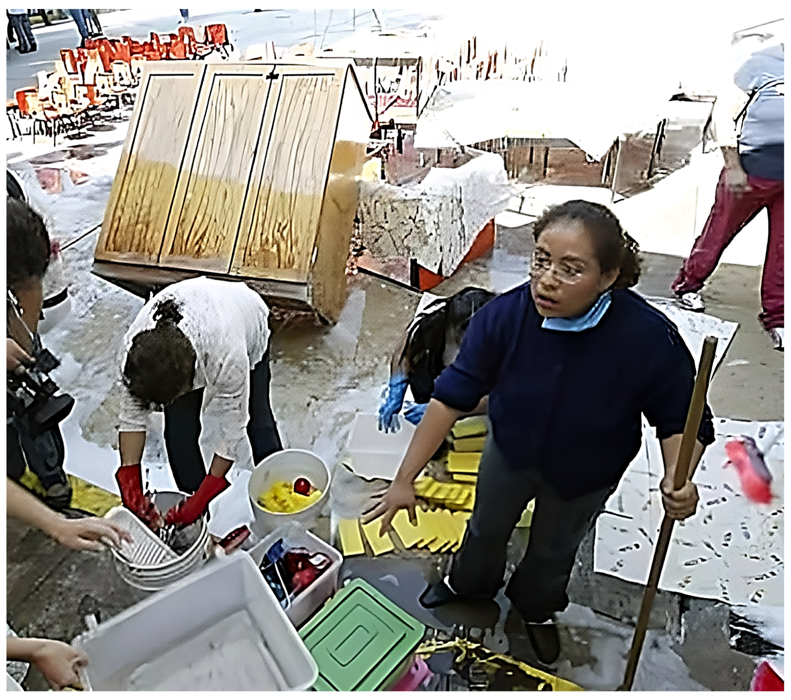
Cuautepec, Edomex has a geography conducive to the occurrence of floods, many of them flash floods that, as they increase, generate flows that descend from the hill upper zones towards the urban area in the lower zones. Constructions located in particular on the left bank of the plain area in the central basin part are flooded when the Cuautepec River overflows, since there is a combined drainage system that carries rainwater and sewage, due mainly to the invasion of the floodplains and the reduction in the hydraulic area of the natural channels in such urban zones. Among dozens of school supplies, books, computers, benches, and children’s games rescued from the mud and garbage that was dragged by the water current that caused the storm on 30 October 2009 in Cuautepec, teachers from the Gertrudis Armendariz and Josefa Ortiz de Domínguez schools exposed to officials, as well as federal and local authorities, that each year, during the rainy season, these centers are flooded by the overflow of the rivers that discharge sewage. In the Josefa Ortiz de Domínguez kindergarten, the teachers lamented the loss of the computer center, where five days later they could still see the 16 computers covered in mud and with traces of the mark of the water level reached by the water that flooded the school.
Seven houses for families that suffered irremediable structural damage were incorporated into the housing improvement program; these houses were located on the left bank of the Cuautepec River near the Precious Blood of Christ Church.
In this regard, José Pérez Castañeda, director of Clean and Urban Image of the Secretariat Services, said that the unit in his charge had so far disposed of 2751 waste tons, including solid waste and household items that were dragged by runoff that descended from the hills to the mild part where the community of Cuautepec is allocated.
Figure 1 shows on furniture the water depth mark reached by the flood inside a kindergarten and it is approximately 1.0 m (photograph from La Jornada newspaper of the event on 30 October 2009 [17]); unfortunately, there was no rainfall measurement, because a pluviograph was not installed in the area surrounding and the kindergarten is located next to the church aforementioned.
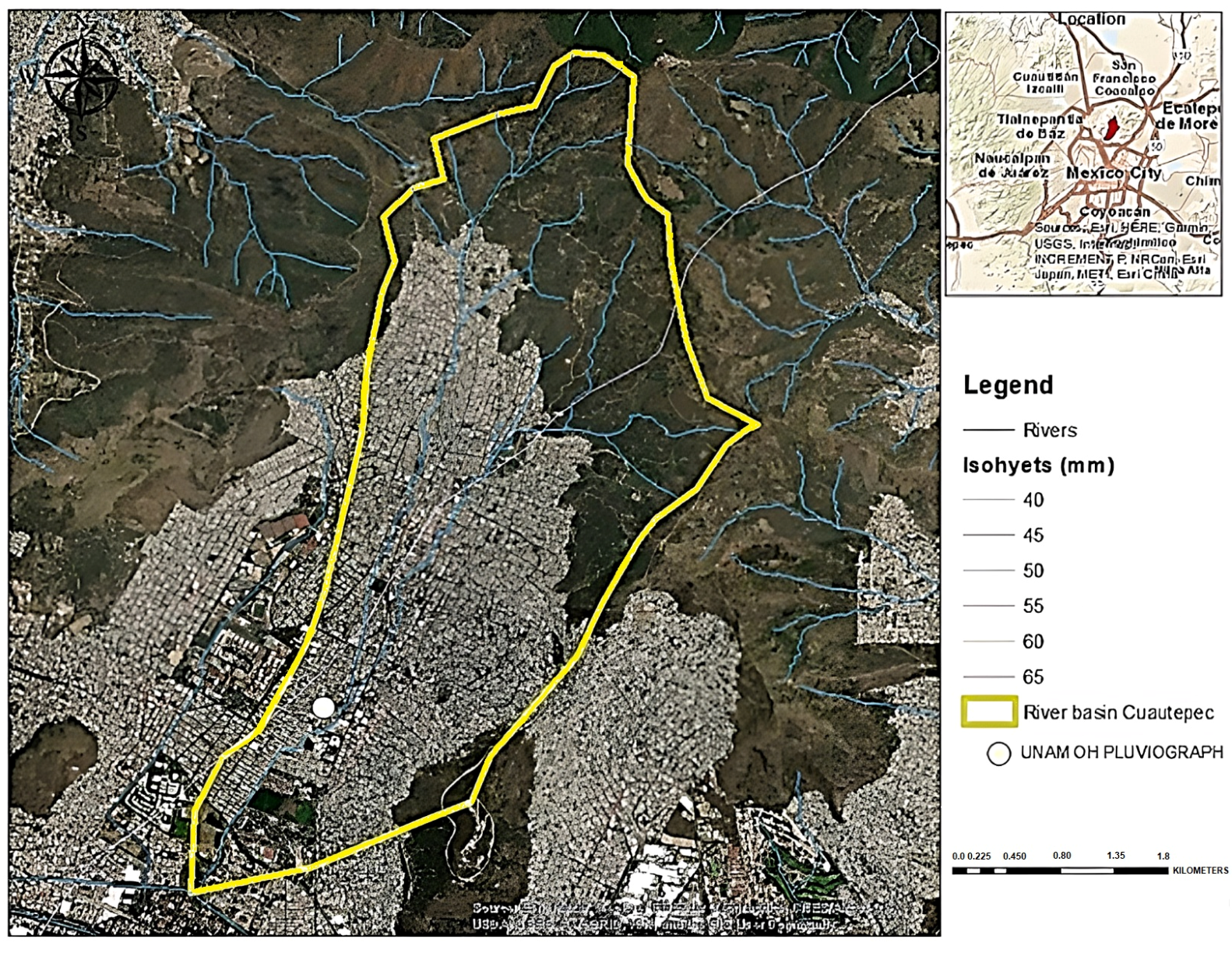
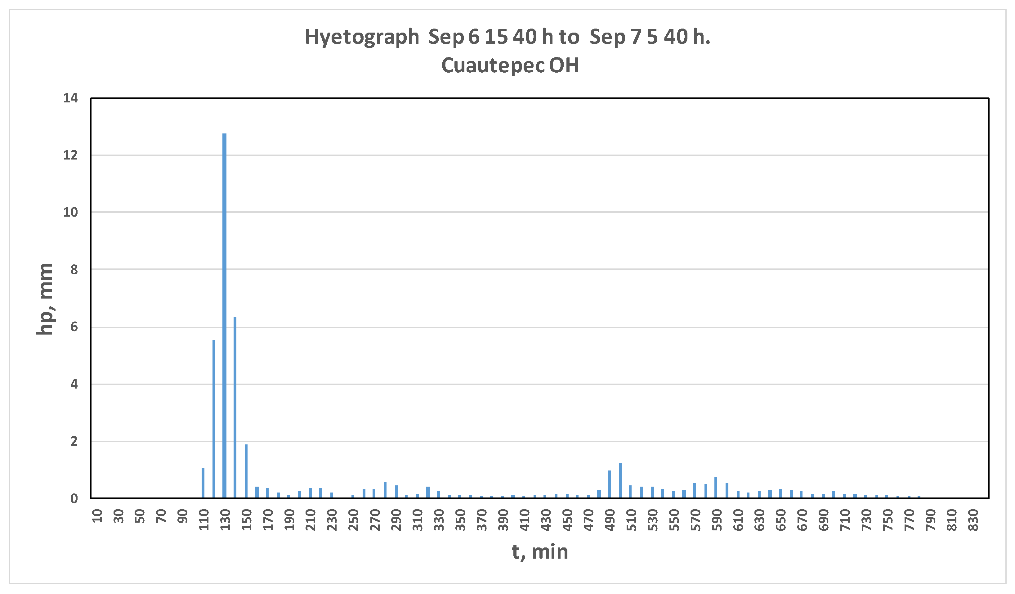
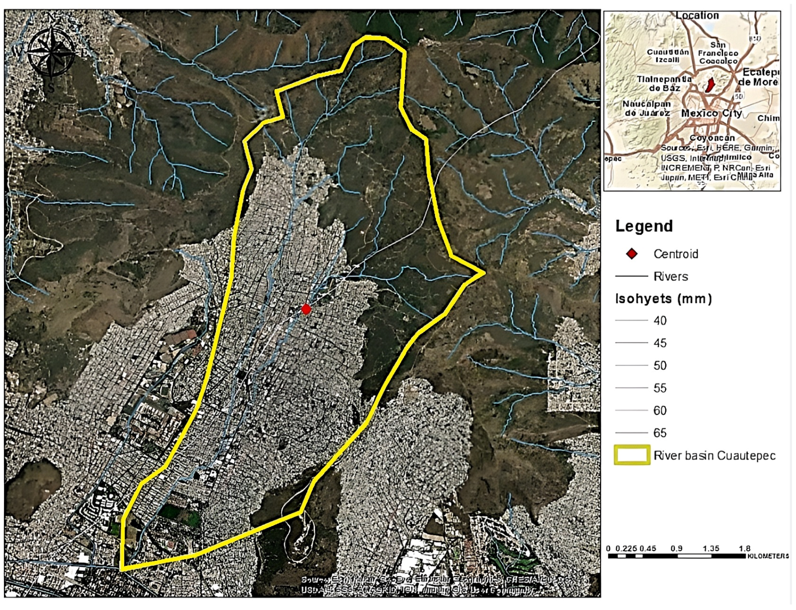
At the end of August 2021 and during the first days of September, storm events occurred, some associated with Hurricane Grace [18,19], that caused severe flooding in several municipalities of Mexico State [20]. The contribution basin of the storm recorded between 3:40 p.m. on 6 September and 5:40 a.m. on 7 September 2021, with a total rainfall of 44.57 mm, is shown in Figure 2; the analyzed basin area is 15 km2, with a main channel length equal to 8.24 km and a main channel slope (dimensionless) of 0.0428, which can lead to supercritical flow conditions. The OH Hydrological Observatory pluviograph of the Institute of Engineering (Figure 2) reported this event that caused a flash flood (Figure 3).
Journalistic sources highlighted at least 2 deaths, nearly 100,000 affected inhabitants, and material damage in 19 different neighborhoods.
2.5. Hydrological Region for Mexico Valley River Basin
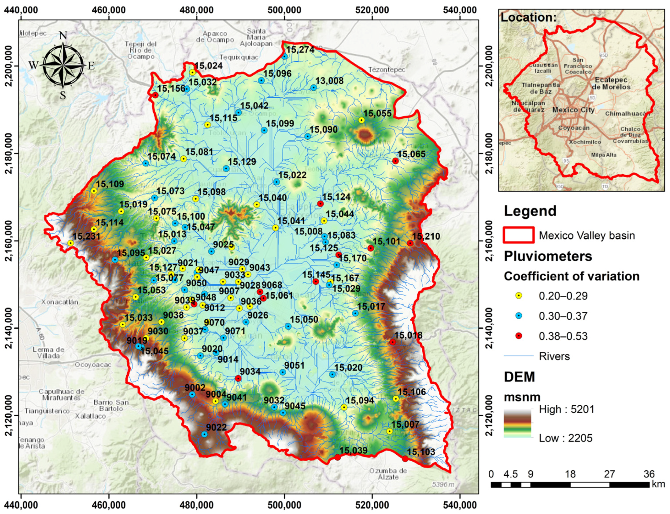
The entire Mexico Valley River Basin (MVRB) hydrology was considered. Since little variation was noted in the variation coefficients for the different stations analyzed in the study by Domínguez et al. [21] (Figure 4), in said study it was reported that the regional function of best data fit, using the procedure described in the methodology, was of the Double Gumbel type [22]; regional factors corresponding to different return periods are highlighted in Table 1.
2.6. Area Reduction Factor Equation
The equation developed by Domínguez et al. [21] was used for the reduction factor per area as a function of the area a of the basin (Equation (3)). The reduction factor per area takes into account the spatial distribution of rainfall.
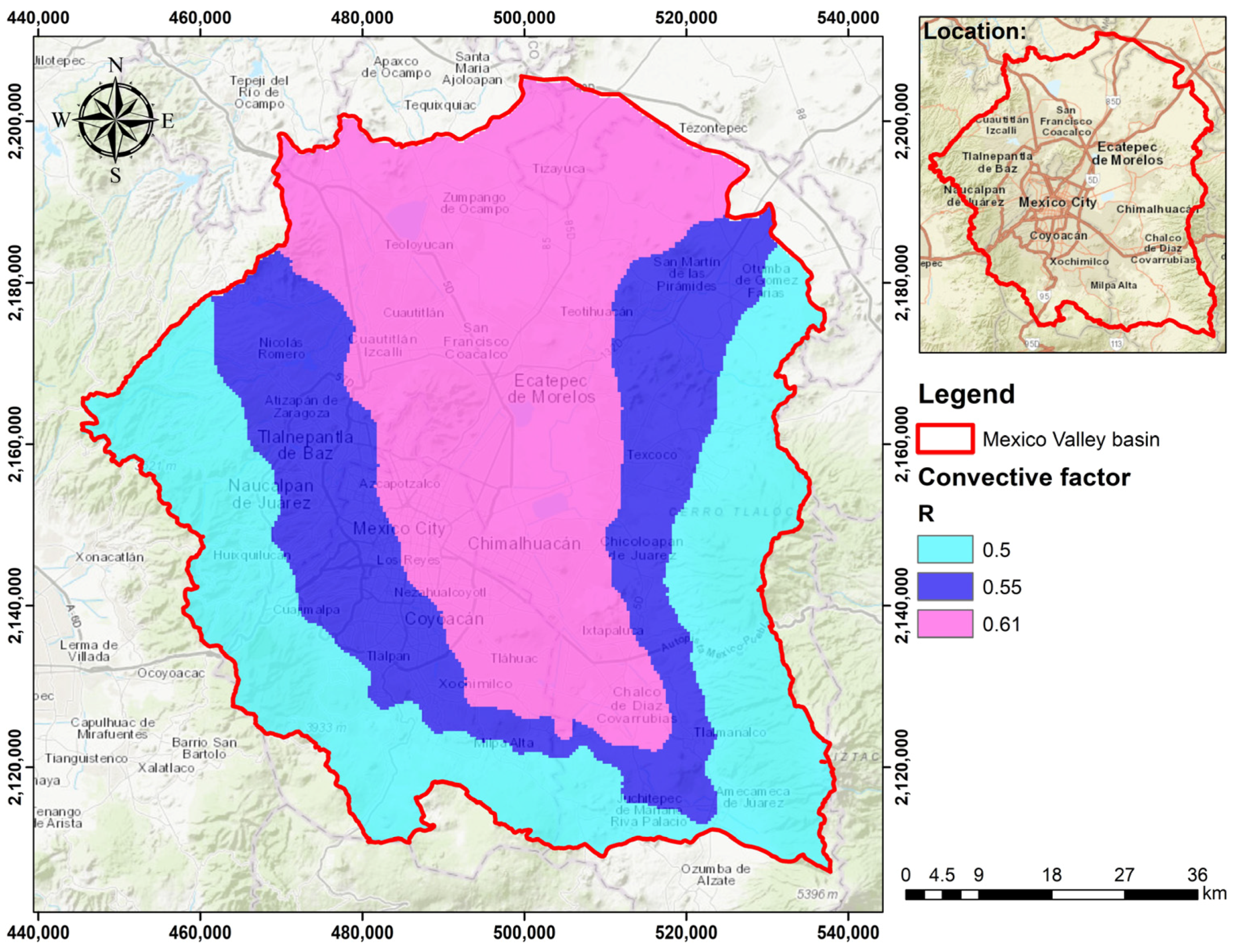
2.7. Convective Factor
2.8. K-Factors to Move to Durations Other than One Hour
K-factors were considered, corresponding to convective factor R, from the modified Chen and Bell [16] version for the study by Domínguez et al. [21]. The K factors allow for obtaining the rainfall that occurs in durations of less than one hour, with respect to the rainfall of one hour.
2.8.1. Hec-HMS Software
The HEC-HMS (Hydrologic Engineering Center–Hydrologic Modeling System) model is a rainfall–runoff model developed by the Hydrologic Engineering Center HEC of the U.S. Army Corps of Engineers USACE that is designed to simulate the runoff hydrograph that occurs at a given point in the river network as a result of a rain event. The predecessor of this model, the HEC-1, was born as an event model and has been considered by many as the most versatile model [23] and probably the most widely used in this type of hydrological characterization of floods.
To calculate evapotranspiration losses, HEC-HMS has different methods. In this case, the method of the SCS Soil Conservation Service, also called the CN curve number, was chosen because it has quality digitized information on the use and type of soil. This method was developed by the SCS of the US Department of Agriculture, USDA, to estimate the losses (or abstractions) in a rain or downpour event [24], and today it is one of the most used in the professional field. In this method, the effective rain height is a function of the total precipitation volume and a loss parameter called the CN curve number. The curve number varies in the range from 0 to 100 and depends on factors that influence the generation of runoff in the basin: hydrological type of soil (hydrological group–drainage capacity); land use and management; soil surface condition; and antecedent moisture condition.
The starting hypotheses or conditioning factors from which the model is based are the following: the simulation is limited to rain events (event model) as a consequence of the application of the model itself to the simulation of floods; the modeling is based on simulating only the direct surface runoff, the base flow is estimated prior to the application of the model; and snow is not taken into account, as we started from events in which there was no snow.
2.8.2. Iber
Iber is a two-dimensional mathematical model for river and estuary flow simulation developed from the collaboration of the Water and Environment Engineering Group, GEAMA (University of La Coruña); the Mathematical Engineering Group (University of Santiago de Compostela); and the Flumen Institute (Polytechnic University of Catalonia and International Center for Numerical Methods in Engineering) and promoted by the Center for Hydrographic Studies of CEDEX. Iber is a numerical model developed directly from the Spanish public administration in collaboration with the aforementioned universities and designed to be especially useful for the specific technical needs of hydrographic confederations in the application of current sectoral legislation on water. Iber’s hydrodynamic module solves the two-dimensional St. Venant equations, incorporating the effects of turbulence and wind surface friction [25].
The shallow water equations and those of the k-ε model are solved using the finite volume method for two-dimensional unstructured grids. The numerical schemes used in Iber are especially suitable for modeling regime changes and dry–wet fronts (flood fronts). The discretization of the spatial domain is carried out with finite volumes in unstructured meshes, admitting these mixed ones formed by triangular and quadrangular elements. The convective flow is discretized using Godunov-type off-center schemes, specifically Roe’s off-center scheme, as well as its depth to order 2 with a slope limiter to avoid oscillations in regions with local maxima or minima. The term that includes the bottom slope is discretized off-center in order to avoid spurious oscillations of the free shell when working with complex terrain. The rest of the source terms, including those of turbulent diffusion, are discretized with a centered scheme.
2.8.3. Hec-Ras 2d
Hec-Ras 2d software, developed by the United States Corps of Engineers [26], has been evolving in its potentialities; Hec-Ras was initially conceptualized for flow in one direction, and already in its two-dimensional form it solves the equations of 2D flow at the free surface for shallow water. The latest versions have incorporated a module that includes the complete two-dimensional moment equations for complete shallow waters, occupies structured grids with digital elevation models that can have high resolution (Lidar type), and considers the Manning N coefficient taking into account different values depending on soil type [27].
3. Results and Discussion
3.1. Flash Flood Hyetographs Obtained for Different Return Periods
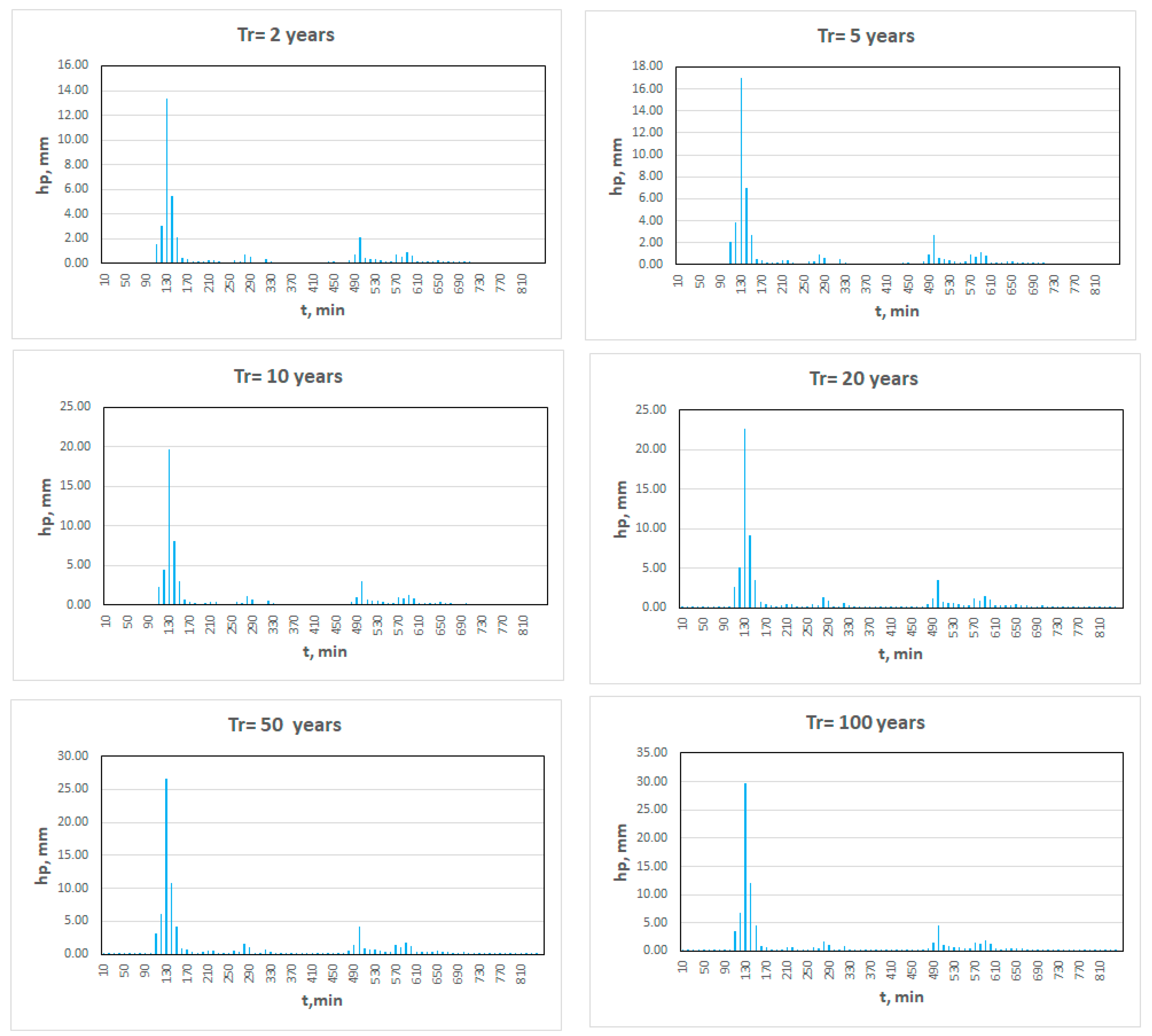
By applying the regionalization procedure before-described and considering an updated map of the historical annual maximum daily mean isohyets of Mexico Valley as well as the basin centroid (Figure 6), a rainfall of 50 mm was estimated for the study site; this rainfall times the regional factor for a given return period results in the design rainfall. Subsequently, said rainfall was reduced to take into account its spatial distribution using the area reduction factor, and later the total rain of one hour and shorter duration was estimated to obtain the mass curve of the design storm. With this information, design hyetographs were determined, considering a duration of 14 h and shaping hyetographs based on behavior of the historical flash flood that was taken as a base. These hydrographs can be seen in Figure 7.
3.2. Simulation of the Historic Flood Using Hec-HMS
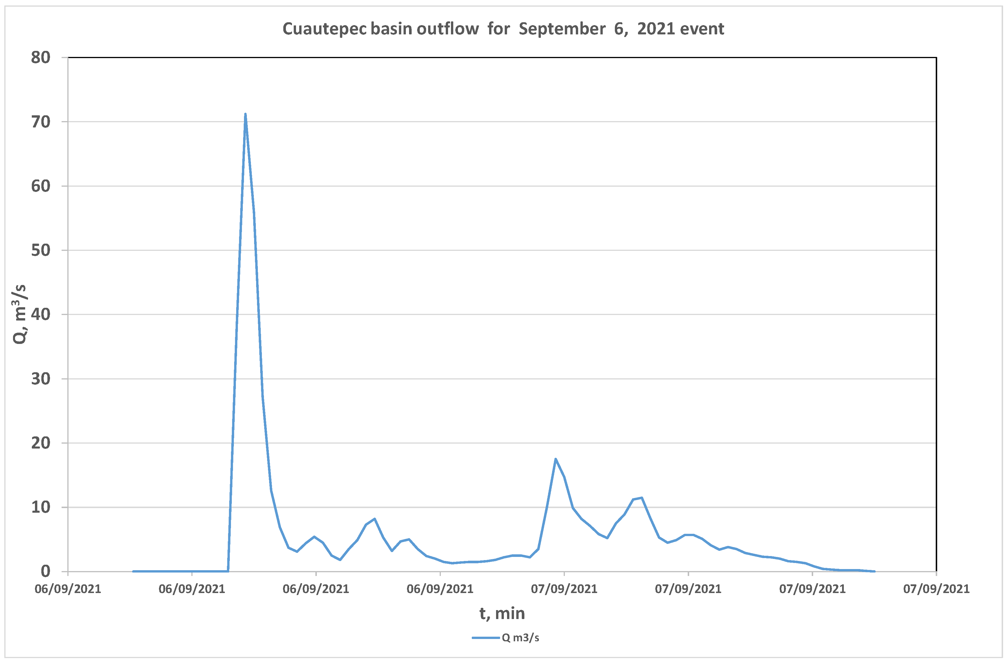
Flood simulation using the Hec-Hms semi-distributed model produced the hydrograph shown in Figure 8.
3.3. Hydrographs Produced by Hyetographs for Different Tr Calculated with Hec-Hms
Hydrographs were obtained using Hec-Hms, and these were compared with the historical storm, as shown in Figure 9.
3.4. Depth and Velocity Maps of Historic Flash Flood
When using Iber software using the historical hydrograph produced by the flash flood obtained with Hec Hms and a calculation time of 24 h, depth and velocity maps created using a calculation time of 13,600 s (3.78 h) are presented in Figure 10; these result were partially due to the high calculation time required by the Iber software to perform processing.
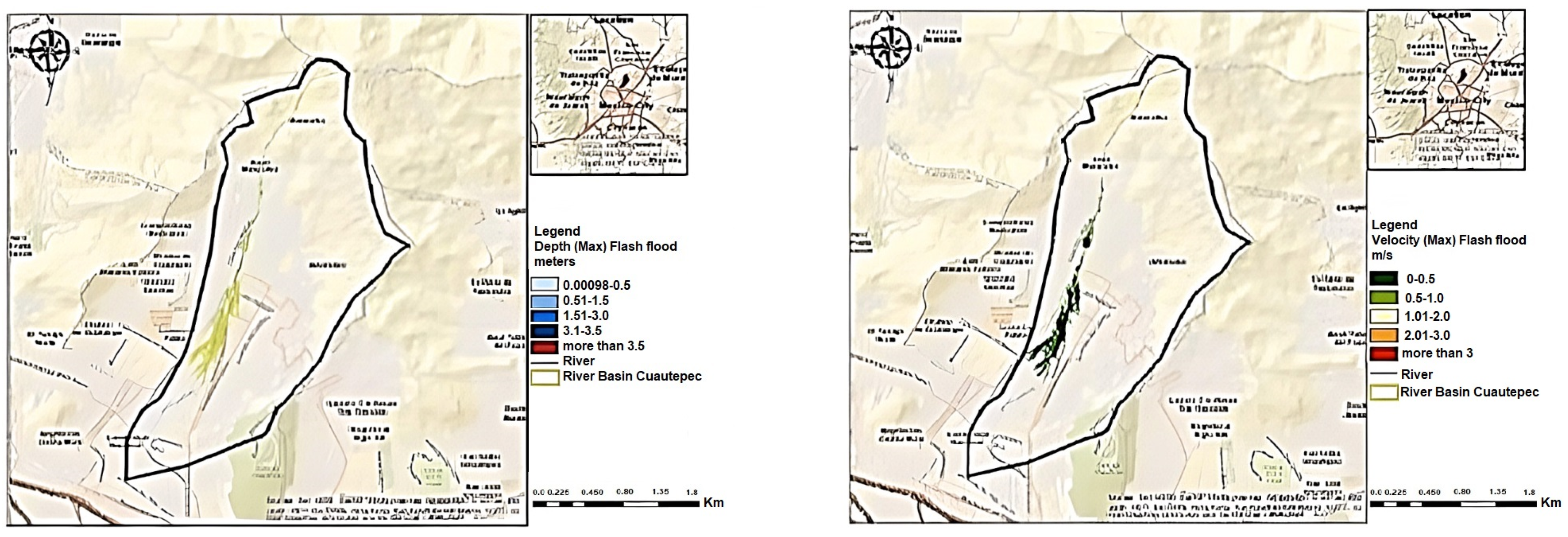
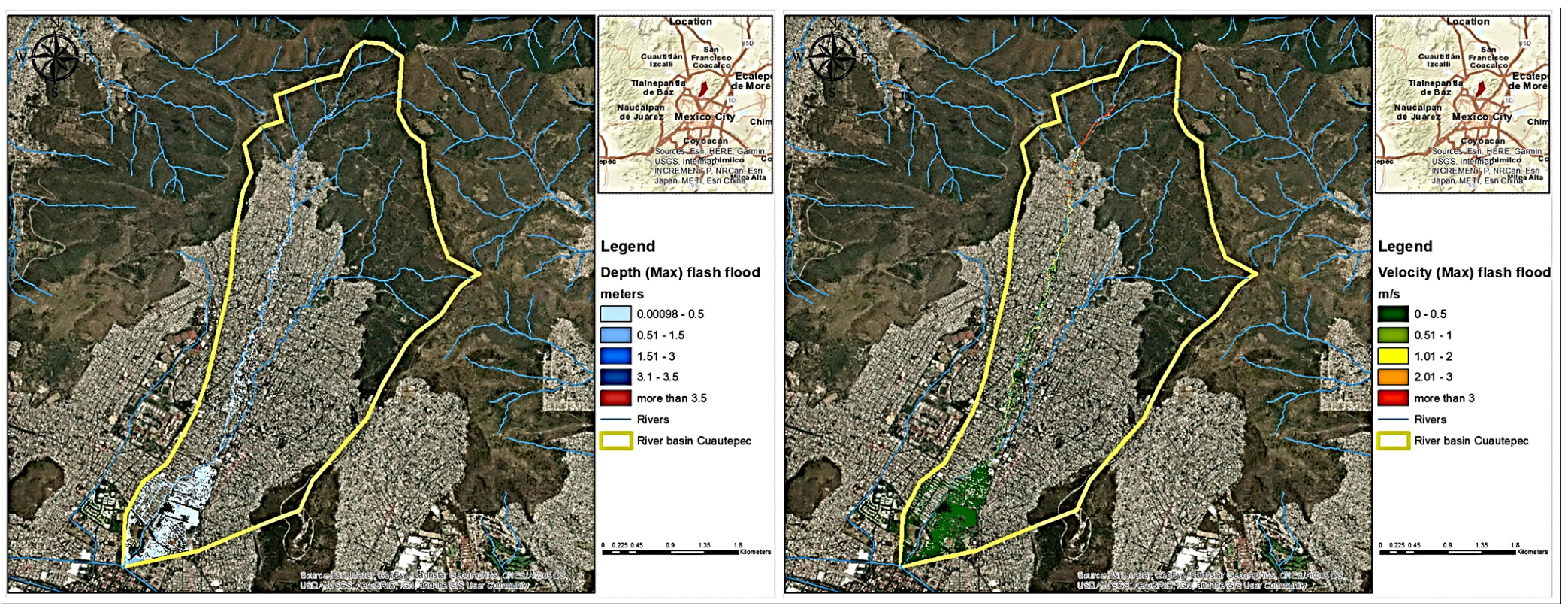
In contrast, when using the Hec-Ras 2d software, simulation was carried out for 7.5 h, and in a calculation time of approximately 23 min, in this case, the depth and velocity maps indicated in Figure 11 were obtained.
The water depths reported using Iber in almost the first 4 h for the runoff process indicate highest values between 1.5 and 3 m and velocity between 3 and almost 9.5 m/s, which gives indications that possible supercritical flow occurred in the event, which could be intuited with main channel slope data (S = 0.0428).
The most extensive simulation (of 7.5 h) carried out by Hec-Ras 2d reported maximum depths of the order of 3.1 m and a maximum velocity that reached 3 m/s; after 6 h, water drained into the basin outlet. The Manning N coefficient was set with different values, according to soil type.
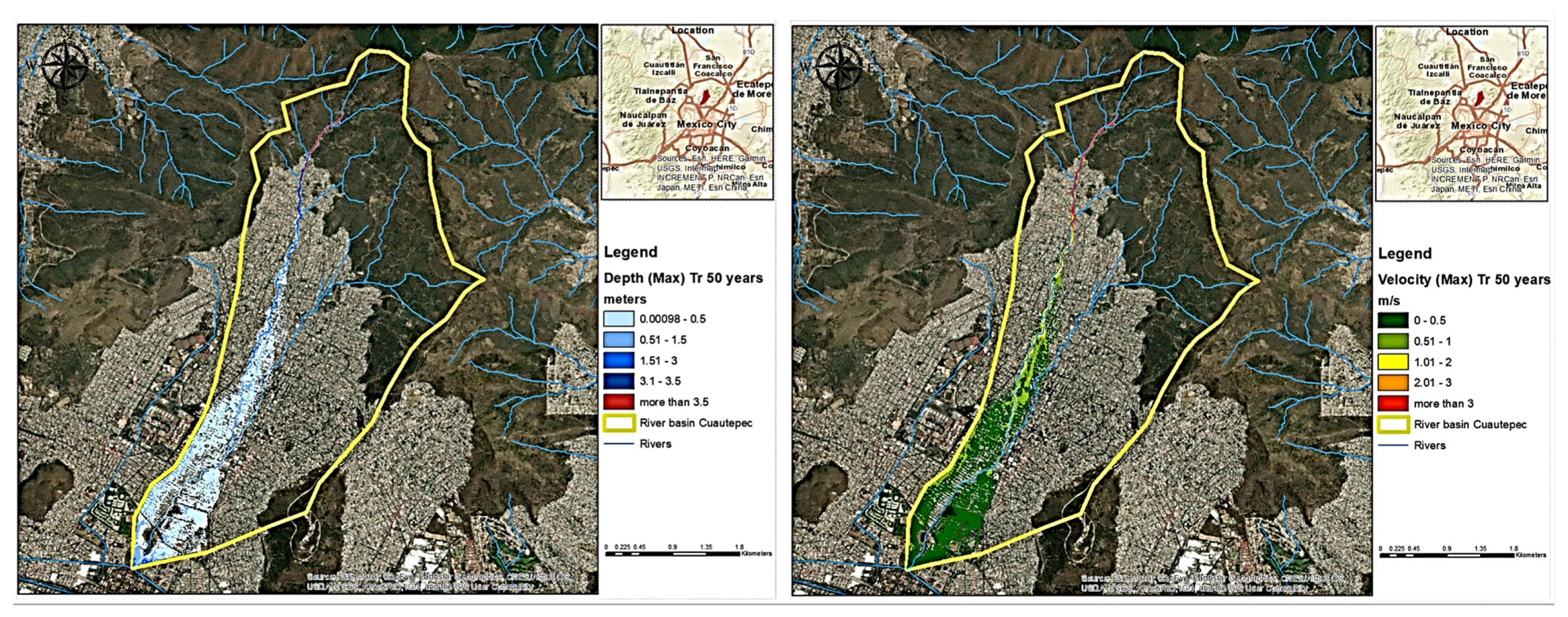
3.5. Flash Flood for Tr = 50 Years
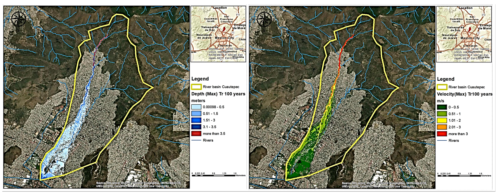
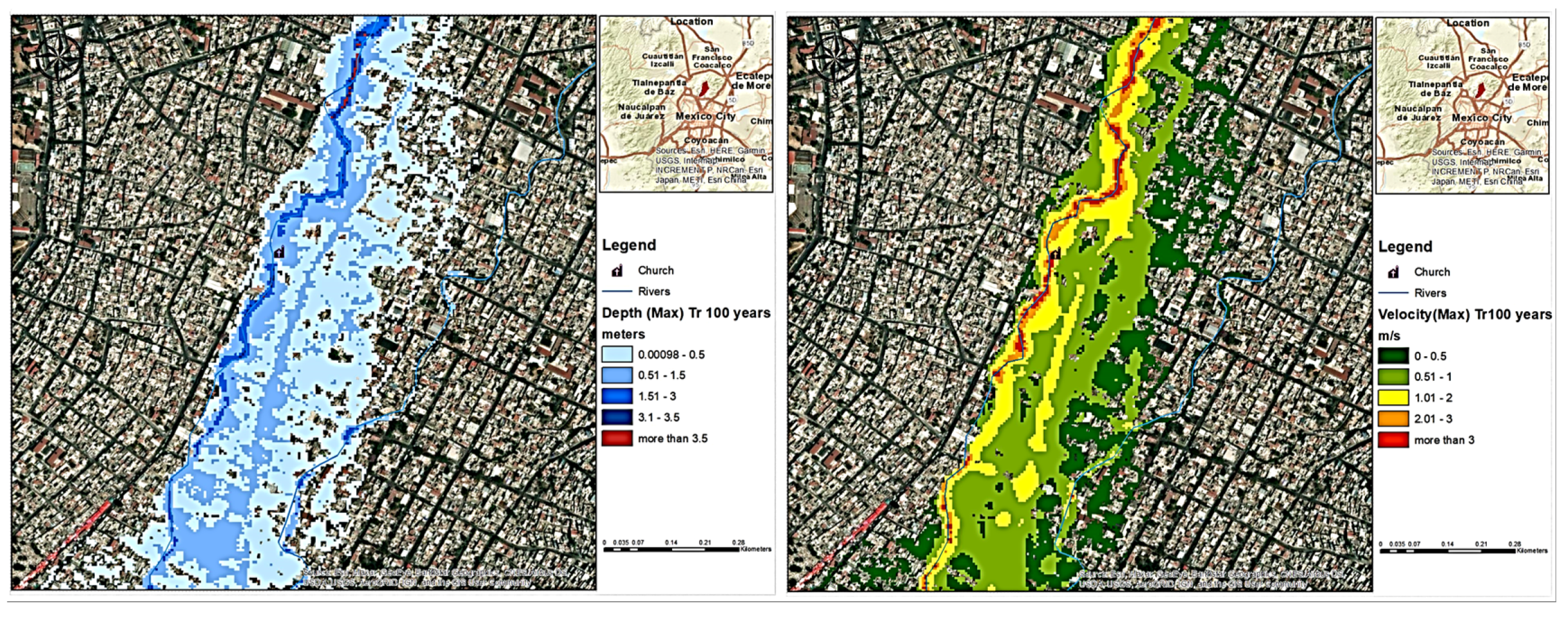
The reported maps and velocities from simulation with Hec-Ras 2d for flash flood for Tr = 50 and Tr=100 years are shown in Figure 12 and Figure 13.
In the case of floods with Tr = 50 and Tr = 100 years, maximum depths would reach 3.5 m or even greater, and velocities would also exceed 3 m/s, which does give an idea of a supercritical flow generated in the study site that increases risk in a flash flood event.
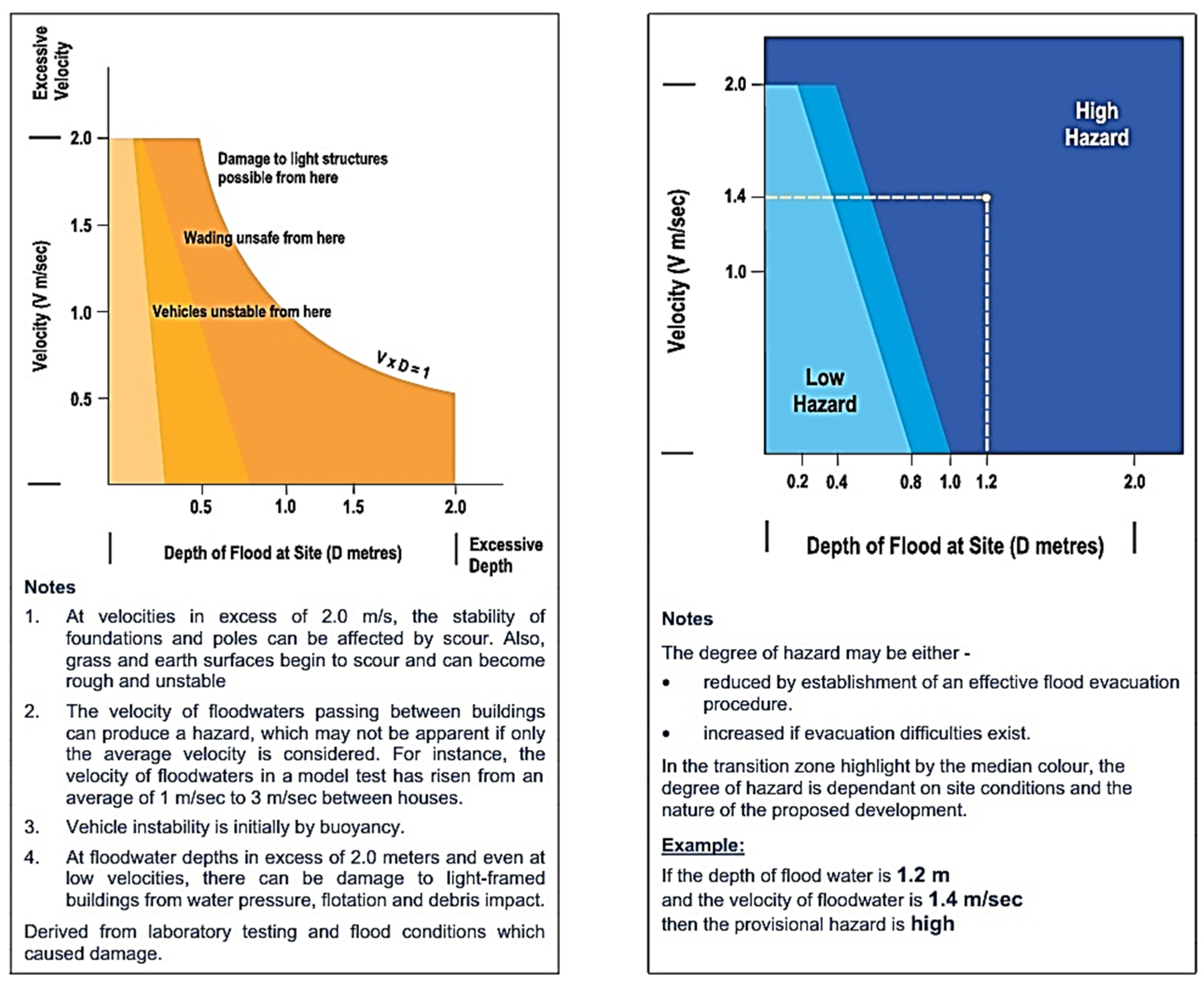
When comparing historical results and floods with Tr = 50 and 100 years with the Dorrigo diagram [28,29,30], which is an indicator of the resistance to overturning (Figure 14), the depths and velocity that occurred in the historical event and for the Tr mentioned above lead to a high to very high probability of overturning or dragging in the water of the objects found in the passage of the current. The occurrence of human and material losses is inevitable in the face of said runoff event attributed to precipitation in the topography of the site that leads to the occurrence of dangerous supercritical flows.
For a finer estimate of the velocities that occurred in the analyzed event, it is advisable to carry out tests with different values of the calculation time interval, since instabilities can be generated in the results of the simulation algorithms. Hydrodynamic models that solve the Saint Venant equations with shock capturing [25,31] can also be used to consider supercritical flows and transitions to subcritical flows. On the other hand, in the case of constant high velocity conditions, even going down the water depth, the danger of tipping objects would still be high, as indicated by the Dorrigo diagram.
Regarding an event associated with a Tr of 100 years, it can be concluded that the braces reached in the area surrounding the kindergarten as well as the constructions on the left bank of the river according to the Hec-Ras 2d modeling are around 1 m, as shown in the evidence of Figure 1 and in the enlargement shown in Figure 15. For the velocity range from 1 to 3 m/s, if we apply Figure 13 in this specific case, it is concluded that for said tie rod there is a very high risk both of resistance to overturning and high danger, as defined in Figure 14.
Additionally, the Tamez criterion [32] establishes that either a combination of depth of 1 m and a velocity of 1 m/s or the factor defined as the product of the depth by the velocity of 0.5 m2/s are sufficient to have a serious danger of loss of humans and damage to the household items of the population.
4. Conclusions
The regionalization application method based on variation coefficients with difference in hyetograph shape construction was useful to obtain direct runoff hydrographs proposed for different return periods. They were created from a historical flash flood from the study site, a kind of event that caused a lot of human and material damages. For both historical and statistical hydrograph simulation purposes, the free-use tool US Army Hec-Ras 2d was very useful since calculation times were relatively short, about 30 min, while the Iber software had problems in calculation time because so many hours were required to perform simulation that we finally decided to not continue to apply it in this investigation. Another inconvenience observed was that boundary conditions were fed with the hydrograph produced by a measured storm, that is, the Iber hydrological module could not be used and Hec-Ras 2d version did not request precipitation data; therefore, it is advisable to delve into improvements to hydrological modules to model rainfall–runoff scenarios. Depth maps and maximum depths obtained revealed that in the face of flash floods for return periods of up to 100 years, the probability of dragging obstacles in the water path is very high and the floodplain is also reflected as being wide. Due to rugged, steep topography in the upper basin, it is prone to flash floods, landslides, and debris, as well as supercritical flow development. Supercritical flows associated with high water velocities are really dangerous since they can cause great damage to infrastructure as well as people dragging, cars overturning, and human losses. Disorganized population growth and the territory, together with land use change, has encouraged construction in these highly dangerous areas. Therefore, the recommendation, in case there is already infrastructure that may be susceptible to being damaged by flash flood events, is the use of structural, such as velocity reducers that change roughness coefficient, temporary, or permanent measures to reduce future damage and continue promoting a culture of warning and prevention to the population.
Author Contributions
Conceptualization, M.A., M.P., F.D.L. and R.D.; methodology R.D., O.S., M.A. and M.P.; validation, M.P. and L.C.; data curation, F.D.L. and M.P.; writing—review and editing, M.A. and M.P.; visualization, F.D.L.; supervision, M.A., M.P. and F.D.L. All authors have read and agreed to the published version of the manuscript.
Funding
This research received no external funding.
Institutional Review Board Statement
Not applicable.
Informed Consent Statement
Not applicable.
Data Availability Statement
Not applicable.
Conflicts of Interest
The authors declare no conflict of interest.
References
- National Weather Service. 2022. Available online: https://www.weather.gov/phi/FlashFloodingDefinition (accessed on 5 November 2022).
- Akstinas, V.; Meilutytė-Lukauskienė, D.; Kriaučiūnienė, J.; Šarauskienė, D. Features and causes of catastrophic floods in the Nemunas River basin. Hydrol. Res. 2020, 51, 308–321. [Google Scholar] [CrossRef]
- Garzón, H.M.G.; Ortega, B.J.; Garrote, R.J. Las avenidas torrenciales en cauces efímeros: Ramblas y abanicos aluviales. Torrential floods in ephemeral streams: Wadies and alluvial fans. Enseñanza Cienc. Tierra 2009, 17, 264–276. [Google Scholar]
- Aroca, J.E. Importancia de las Abstracciones Iniciales para la Génesis de Avenidas en Cuencas de Montaña. Master’s Thesis, Universidad de Cantabria, Cantabria, Spain, 2014; 50p. [Google Scholar]
- Green, W.H.; Ampt, G.A. Studies on soil physics: Part, I. The flow of air and water through soils. J. Agric. Sci. 1911, 4, 1–24. [Google Scholar]
- Liu, J.; Zhang, J.; Feng, J. Green–Ampt model for layered soils with nonuniform initial water content under unsteady infiltration. Soil Sci. Soc. Am. J. 2008, 72, 1041–1047. [Google Scholar] [CrossRef]
- Vannasy, M.; Nakagoshi, N. Estimating Direct Runoff from Storm Rainfall Using NRCS Runoff Method and GIS Mapping in Vientiane City, Laos. Int. J. Grid Distrib. Comput. 2016, 9, 253–266. [Google Scholar] [CrossRef]
- Karbasi, M.; Shokoohi, A.; Saghafian, B. Loss of Life Estimation Due to Flash Floods in Residential Areas using a Regional Model. Water Resour. Manag. 2018, 32, 4575–4589. [Google Scholar] [CrossRef]
- Aristizábal, E.; Arango, C.M.I.; García, L.I.K. Definición y clasificación de las avenidas torrenciales y su impacto en los Andes colombianos. Cuad. Geogr. Rev. Colomb. Geogr. 2020, 1, 242–258. [Google Scholar] [CrossRef] [Green Version]
- Bilasco, S.; Hognogi, G.G.; Ros, C.S.; Pop, A.M.; Iuliu, V.; Fodorean, I.; Marian-Potra, A.C.; Sestras, P. Flash Flood Risk Assessment and Mitigation in Digital-Era Governance Using Unmanned Aerial Vehicle and GIS Spatial Analyses Case Study: Small River Basins. Remote Sens. 2022, 14, 2481. [Google Scholar] [CrossRef]
- Shuvo, S.D.; Rashid, T.; Panda, S.K.; Das, S.; Abdul, Q.D. Forecasting of pre-monsoon flash flood events in the northeastern Bangladesh using coupled hydrometeorological NWP modelling system. Meteorol. Atmos Phys. 2021, 133, 1603–1625. [Google Scholar] [CrossRef]
- Kim, E.; Choi, H. Assessment of Vulnerability to Extreme Flash Floods in Design Storms. Int. J. Environ. Res. Public Health 2011, 8, 2907–2922. [Google Scholar] [CrossRef] [PubMed] [Green Version]
- Kong, F.; Huang, W.; Wang, Z.; Song, X. Effectof Unit Hydrographs and Rainfall Hyetographs on Critical Rainfall Estimates of Flash Flood. Adv. Meteorol. 2020, 2020, 2801963. [Google Scholar] [CrossRef]
- Domínguez, R.R.; Carrizosa, E.E.; Fuentes-Mariles, G.E.; Arganis-Juárez, M.L.; Osnaya, J.O.; Galván, T.A. G Análisis regional para la estimación de precipitaciones de diseño en la República Mexicana Regional Analysis in approaching design rainfall in Mexican Republic. Tecnol. Cienc. Agua. 2018, 9, 5–29. [Google Scholar] [CrossRef]
- Hec-HMS. 2022. Available online: https://www.hec.usace.army.mil/software/hec-hms/ (accessed on 3 November 2022).
- Chen, C.L. Rainfall Intensity-Duration-Frequency Formulas. J. Hydraul. Eng. 1982, 109, 1603–1621. [Google Scholar] [CrossRef]
- La Jornada. 2022. Available online: https://www.jornada.com.mx/2009/11/04/capital/032n1cap (accessed on 1 November 2022).
- Milenio. 2021. Available online: https://www.milenio.com/politica/comunidad/declaran-desastre-natural-27-municipios-afectaciones-grace (accessed on 1 November 2022).
- La Silla Rota. 2021. Available online: https://lasillarota.com/hidalgo/estado/2021/9/8/por-inundaciones-en-tula-el-mezquital-mil-casas-danadas-15-decesos-295643.html (accessed on 2 November 2022).
- El País. 2021. Available online: https://elpais.com/mexico/2021-09-07/al-menos-dos-muertos-tras-una-fuerte-tormenta-en-ecatepec.html (accessed on 2 November 2022).
- Domínguez, R.; Carrizosa, E.; Arganis, M.; Santana, A.; De Luna, F.; Mendoza, R.; Hernández, D.; González, S.; Vázquez, R.; Hernández, A. Proyectos y Estudios para Mejorar la Infraestructura de Drenaje, Actualización del Manual de obras Hidráulicas de la Ciudad de México; Technical Report; Informe Técnico para SACMEX: Mexico City, Mexico, 2022. [Google Scholar]
- González. Contribución al Análisis de Frecuencias de Valores Extremos de los Gastos Máximos en un Río; Serie Azul; Instituto de Ingeniería, UNAM: Mexico City, Mexico, 1970. [Google Scholar]
- Bedient, P.B.; Huber, W.C. Hydrology and Floodplain Analysis; Addison-Wesley: Boston, MA, USA, 1992. [Google Scholar]
- Mockus, V. National Engineering Handbook, Section 4: Hydrology; United States Department of Agriculture (USDA), Soil Conservation Service (SCS): Washington, DC, USA, 1969. [Google Scholar]
- Bladé, E.; Cea, L.; Corestein, G.; Escolano, E.; Puertas, J.; Vázquez-Cendón, E.; Dolz, J.; Coll, A. Iber: Herramienta de simulación numérica del flujo en ríos. Rev. Int. Métodos Numéricos Cálculo Diseño Ing. 2014, 30, 1–10. [Google Scholar] [CrossRef] [Green Version]
- Available online: https://www.hec.usace.army.mil/software/hec-ras/ (accessed on 10 November 2022).
- Costabile, P.; Costanzo, C.; Ferraro, D.; Macchione, F.; Petaccia, G. Performances of the New HEC-RAS Version 5 for 2-D Hydrodynamic-Based Rainfall-Runoff Simulations at Basin Scale: Comparison with a State-of-the Art Model. Water 2020, 12, 2326. [Google Scholar] [CrossRef]
- NSW. Floodplain Development Manual, the Management of Flood Liable Land; News South Wales Government, Department of Infrastructure, Planning and Natural Resources: Sidney, NSW, Australia, 2005. [Google Scholar]
- CONAGUA. Lineamiento para la Elaboración de Mapas de Peligro por Inundación; GASIR: Mexico City, México, 2014. [Google Scholar]
- Velez, M.L.; Fuentes, M.; Rubio, G.H.; De Luna, C.F. Flood hazard maps as a tool for assessing the risk of damage to homes. In Proceedings of the XXIII National Hydraulic Congress, Puerto Vallarta, Jalisco, Mexico, 14 October 2014. [Google Scholar]
- Musolino, G.; Ahmadian, R.; Xia, J.; Falconer, R.A. Mapping the danger to life in flash flood events adopting a mechanics based methodology and planning evacuation routes. J. Flood Risk Manag. 2019, 1, e12627. [Google Scholar] [CrossRef]
- Nanía, L.S.; León, A.S.; García, M.H. Hydrologic-Hydraulic Model for Simulating Dual Drainage and Flooding in Urban Areas: Application to a Catchment in the Metropolitan Area of Chicago. J. Hydrol. Eng. 2015, 20, 04014071. [Google Scholar] [CrossRef]
Figure 1.
Water depth reached, observed on furniture at the affected site after flood event of 30 October 2009. Source: Google images.
Figure 1.
Water depth reached, observed on furniture at the affected site after flood event of 30 October 2009. Source: Google images.

Figure 2.
Location of the study site and the pluviograph of the OH, UNAM.

Figure 3.
Flash flood hyetograph that occurred in September 2021 in Mexico State, Mexico.

Figure 4.
Coefficients map of variation for historical annual maximum daily rainfall in Mexico Valley. “Adapted from Ref. [21], 2022, SACMEX”.
Figure 4.
Coefficients map of variation for historical annual maximum daily rainfall in Mexico Valley. “Adapted from Ref. [21], 2022, SACMEX”.

Figure 5.
Convective factor R Map for Mexico Valley River Basin. “Adapted from Ref. [21], 2022, SACMEX”.
Figure 5.
Convective factor R Map for Mexico Valley River Basin. “Adapted from Ref. [21], 2022, SACMEX”.

Figure 6.
Estimation of the historical annual maximum daily average rainfall for the study site.

Figure 7.
Hyetographs for flash floods. Cuautepec Basin Tr = 2, 5, 10, 20, 50 and 100 years.

Figure 8.
Flash flood hydrograph produced by the historic storm of September 2021. Estimated with Hec-HMS. Cuauhtepec Basin, Edomex.
Figure 8.
Flash flood hydrograph produced by the historic storm of September 2021. Estimated with Hec-HMS. Cuauhtepec Basin, Edomex.

Figure 9.
Estimated hydrographs for storms with different Tr and historical flash flood.

Figure 10.
Depths and velocity maps, historical flash flood using Iber t = 13,600 s (3.78 h).

Figure 11.
Depths and maximum velocity, maps for Historic flash flood using Hec-Ras2d.

Figure 12.
Depths and max velocity, maps for Tr 50 years using Hec-Ras2d.

Figure 13.
Maps of depths and maximum velocity for Tr 100 years using Hec-Ras2d.

Figure 14.
Hazard according to depth vs. velocity of water relationship and its categorization. Source: New South Wales, 2005.
Figure 14.
Hazard according to depth vs. velocity of water relationship and its categorization. Source: New South Wales, 2005.

Figure 15.
Floodplain expansion for flash flood with Tr = 100 years.


Table 1.
Dimensionless regional factors for estimating annual maximum daily rainfall for different return periods Tr in years for Mexico Valley River Basin. “Information consulted from Ref. [21], 2022, SACMEX” Source: [21].
| Tr, Years | CVM (D-GUMBEL) |
|---|---|
| 2 | 0.94 |
| 5 | 1.2 |
| 10 | 1.39 |
| 20 | 1.59 |
| 50 | 1.88 |
| 100 | 2.09 |
| 200 | 2.29 |
| 500 | 2.56 |
| 1000 | 2.76 |
| 2000 | 2.97 |
| 5000 | 3.23 |
| 10,000 | 3.44 |
Disclaimer/Publisher’s Note: The statements, opinions and data contained in all publications are solely those of the individual author(s) and contributor(s) and not of MDPI and/or the editor(s). MDPI and/or the editor(s) disclaim responsibility for any injury to people or property resulting from any ideas, methods, instructions or products referred to in the content. |
© 2023 by the authors. Licensee MDPI, Basel, Switzerland. This article is an open access article distributed under the terms and conditions of the Creative Commons Attribution (CC BY) license (https://creativecommons.org/licenses/by/4.0/).
Share and Cite
MDPI and ACS Style
Arganis, M.; Preciado, M.; Luna, F.D.; Cruz, L.; Domínguez, R.; Santana, O. Application of a Regionalization Method for Estimating Flash Floods: Cuautepec Basin, Mexico. Water 2023, 15, 303. https://doi.org/10.3390/w15020303
AMA Style
Arganis M, Preciado M, Luna FD, Cruz L, Domínguez R, Santana O. Application of a Regionalization Method for Estimating Flash Floods: Cuautepec Basin, Mexico. Water. 2023; 15(2):303. https://doi.org/10.3390/w15020303
Chicago/Turabian StyleArganis, Maritza, Margarita Preciado, Faustino De Luna, Liliana Cruz, Ramón Domínguez, and Olaf Santana. 2023. "Application of a Regionalization Method for Estimating Flash Floods: Cuautepec Basin, Mexico" Water 15, no. 2: 303. https://doi.org/10.3390/w15020303
Note that from the first issue of 2016, this journal uses article numbers instead of page numbers. See further details here.