
Fine-Scale Assessment of Greenhouse Gases Fluxes from a Boreal Peatland Pond
1
Key Laboratory of Sustainable Forest Ecosystem Management—Ministry of Education, School of Forestry, Northeast Forestry University, Harbin 150040, China
2
Heilongjiang Sanjiang Plain Wetland Ecosystem Research Station, Fuyuan 156500, China
3
Key Laboratory of Wetland Ecology and Environment, Northeast Institute of Geography and Agroecology, Chinese Academy of Sciences, Changchun 130102, China
*
Author to whom correspondence should be addressed.
Water 2023, 15(2), 307; https://doi.org/10.3390/w15020307
Submission received: 7 November 2022
/
Revised: 6 January 2023
/
Accepted: 7 January 2023
/
Published: 11 January 2023
(This article belongs to the Section Water and Climate Change)
Abstract
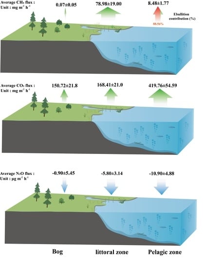
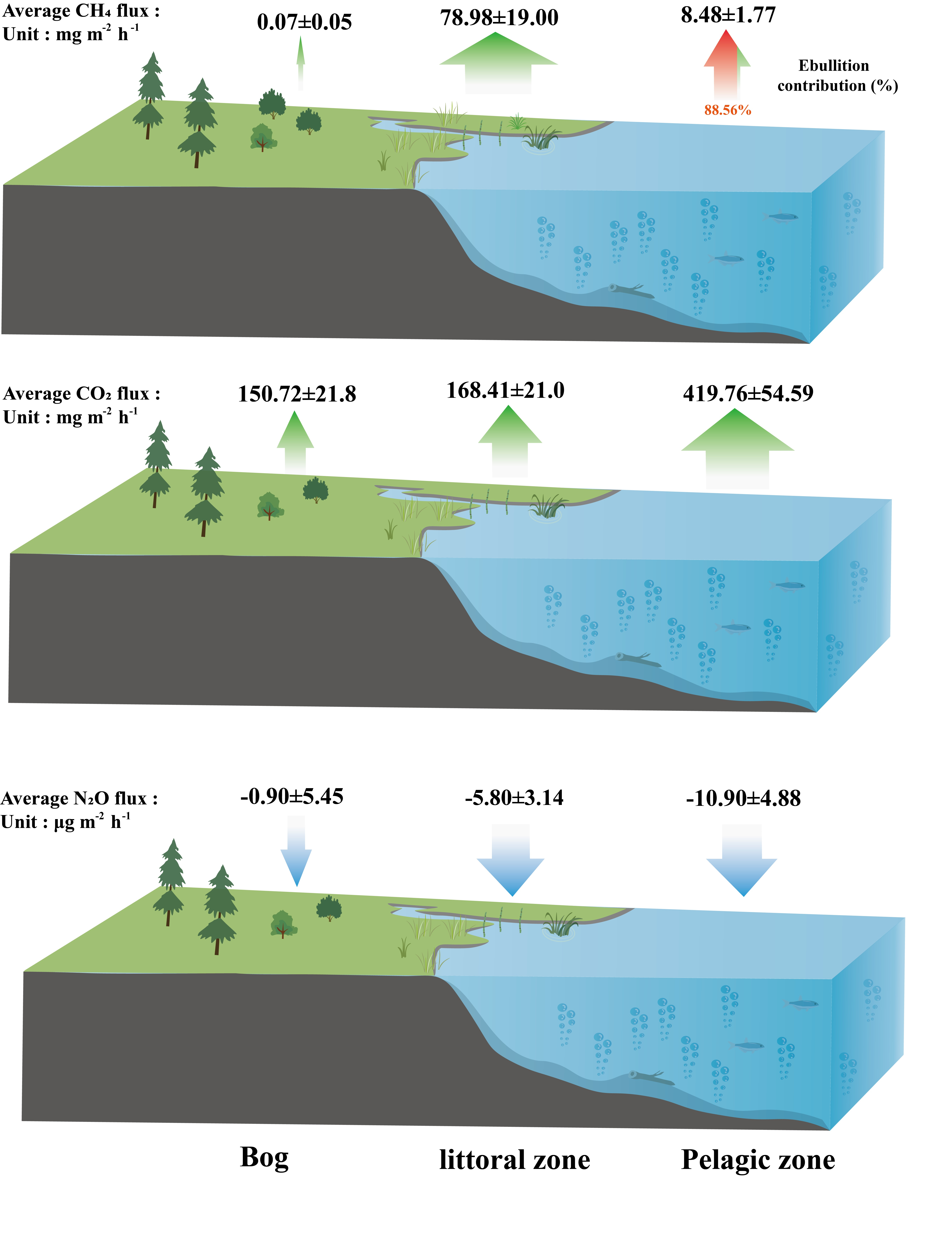
:Ponds are abundant in the boreal peatland landscape, which are potential hotspots for greenhouse gas (GHG) emissions. However, compared to large lakes, ponds are difficult to identify by satellite, and they have not been adequately studied. Here, we observed methane (CH4), carbon dioxide (CO2), and nitrous oxide (N2O) fluxes in the growing season at three sites along the water table gradient from the pelagic zone, littoral zone and bog across a shallow pond in a boreal peatland landscape in Northeastern China. The results showed that the littoral zone, dominated by herb Carex, was the hotspot for CH4 emissions. CH4 fluxes in littoral zone averaged 78.98 ± 19.00 mg m−2 h−1. The adjacent bog was a weak source of CH4 emissions, with an average flux of 0.07 ± 0.05 mg m−2 h−1. Within the pond, CH4 was mainly emitted through ebullition, accounting for 88.56% of the total CH4 fluxes, and the ebullition fluxes were negatively correlated with dissolved oxygen (DO). CO2 fluxes were highest in the pelagic zone, with an average of 419.76 ± 47.25 mg m−2 h−1. Wind and strong sediment respiration were key factors that led to the high fluxes. The observed three sites were all atmospheric N2O sinks ranging from −0.92 to −10.90 μg m−2 h−1. This study highlights the spatial variation in greenhouse gas fluxes from the pond and its adjacent bog, ignoring the ecotone area may underestimate CH4 fluxes. Although ponds are a hotspot for CH4 and CO2 emissions, they can also be a sink for N2O, which provides a reference for the quantification of global pond GHG fluxes. Therefore, finer-scale in situ observations are necessary to better understand the feedback of permafrost peatland ponds to global warming.
1. Introduction
Greenhouse gases (GHGs), including methane (CH4), carbon dioxide (CO2) and nitrous oxide (N2O), are critical to global warming [1]. By 2019, the atmospheric concentrations of these three gases reached 1877 ± 2 ppb, 410.5 ± 0.2 ppm and 332.0 ± 0.1 ppb, respectively, 260%, 148% and 123% of the preindustrial levels [2]. As an important source of GHG emissions, lakes, despite covering only 3.7% of the Earth’s non-glaciated land area [3], can release 55.8 Tg of CH4, 0.3 Pg of CO2 and 0.27 Tg of N2O per year [4,5,6], which play an essential role in the global GHG budget [4,7]. However, it remains difficult to accurately quantify the GHGs balance of lakes due to the high spatiotemporal variability of their GHG emissions. In particular, for small lakes or ponds [3,8,9], which cannot be identified by satellites, GHG emissions can account for up to 37% of global lake emissions and make a significant contribution to regional GHG emissions [6]. Therefore, precise quantification of GHG fluxes from these small lakes or ponds is needed [10].
In contrast to large lakes, small lakes or ponds are usually shallow, with a higher perimeter to margin ratios and large inflows of lights and nutrients [11]; this enhances anaerobic decomposition in the sediments and leads to more CH4 release from ponds to the atmosphere [12]. The carbon-rich sediments in the pond are directly contacted with the upper mixed water column [13] and consume a large amount of oxygen to produce CO2 through respiration, making small ponds a source of CO2 emissions [8]. In general, small ponds are also sources of N2O emissions. Two key biochemical processes, nitrification and denitrification, control the production of N2O in aquatic ecosystems [14]. However, recent studies have shown that relatively pristine inland water bodies also act as N2O sinks [15].
CH4, CO2 and N2O can be released from lakes through three pathways—first, through diffusive transport. It is a process that depends on the concentration gradient and the velocity of gas exchange. Diffusion is the main way of CO2 and N2O emissions in water [16,17,18]. Second, they can be released through ebullition, which is considered to be an important pathway for CH4 emissions [19,20]. The CO2 and N2O fluxes from ebullition are often less than 0.1% of the diffusion flux [21]; these emissions are usually negligible. When the water surface is covered by vegetation, the transport of plants is the third pathway for GHG emissions. The aerenchyma of plants promotes GHG emissions [22,23].
Accumulation of GHGs in lakes/ponds are often associated with their terrestrial connectivity [24,25]. As the ecotone between terrestrial and aquatic ecosystems. It is worth noting that the littoral zone, is often considered a ‘hotspot’ for GHG emissions [26,27]. The high productivity and material input of plants in the littoral zone provides the conditions for GHG production [12,23]. In the case of humic lakes, the metabolism of the whole lake is closely linked to the littoral vegetation [28]. During the growing season, the littoral zone is the main source of GHGs emissions, accounting for more than 50% of the total emissions from the lake [23,29,30]. Therefore, the littoral zone should also be taken into account when estimating lakes/ponds’ carbon fluxes.
To improve the understanding of fine-scale spatiotemporal variation in GHG dynamics, we selected a pond in a boreal peatland landscape of northeast China, which is located at the southern margin of the Eurasian permafrost, to observe GHG fluxes from the pond and its peatland landscape. The thinner permafrost layer and higher soil temperatures make ecosystems in this region more sensitive to climate warming [31]. The main aims of the study are to (1) determine the spatial and temporal variations in CH4, CO2 and N2O fluxes from the pond during the growing season; (2) determine which environmental factors control the GHG (CH4, CO2, N2O) emissions and (3) assess the dominant CH4 emissions pathway within the pond.
2. Materials and Methods
2.1. Site Description
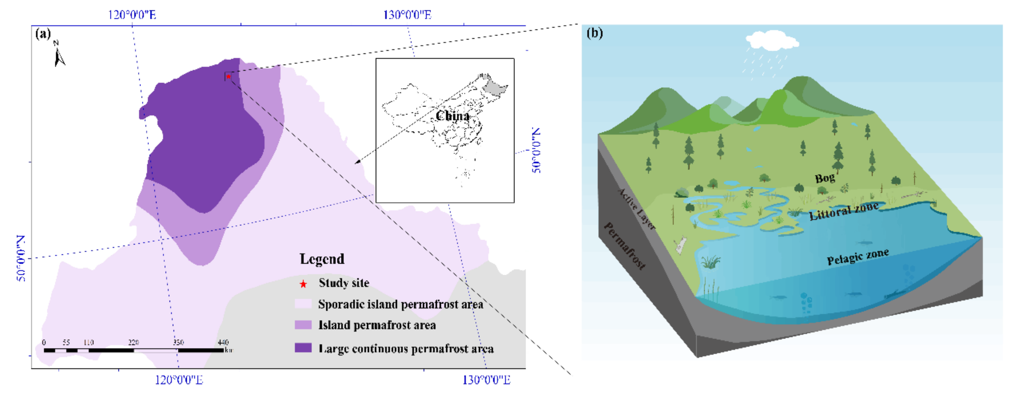
The study area was located in the north of the Great Hing’an Mountains in China, the southern margin of the Eurasian permafrost zone (Figure 1). Most of the boreal peatlands in China are located in this region. Peatlands are widely distributed in flat valleys where rivers meander through [32]. The climate of the region is a cold-temperate monsoon climate with an average annual temperature of −3.8 °C and average annual precipitation of 460.8 mm. Precipitation from June to August often accounts for more than 60% of the annual precipitation. Our studied pond was a shallow humic pond (1200 m2 in the area with maximal depth 1.6 m) in the lowland peatland area (53°00′58″ N, 123°30′29″ E; 574 m a.s.l.). The pond catchment area came from a bog on more elevated ground, and there was an outlet to the northeast of the pond, which flows into an adjacent stream. The active layer reached a maximum in late August (Table 1).
There were no plants in the pelagic zone (Table 1). Species of trees in the bog included Larix gmelinii, Betula fruticosa and occasional Betula platypyhlla. Shrubs in the bog were Ledum palustre, Vaccinium uliginosum, Salix rosmarinifolia, Ribes procumbens, Rubus arcticus and Potentilla fruticosa. The understory herbs in the bog were Calamagrostis angustifolia, Carex lithophila, Habenaria linearifolia, Equisetum sylvaticum and Saussurea manshurica. Sphagnum mainly includes Sphagnum nemoreum and Sphagnum squarrosum. Common plants in the littoral zone were Carex orthostachys, Carex schmidtii and Carex callitrichos. Three observation points were 10 m away from each other.
2.2. Gas Flux Measurement
In the growing season (12 June–26 September 2021), GHGs were measured on a weekly schedule. PVC static chambers size 50 cm × 50 cm × 50 cm were used for bog and littoral zone. Three flux measurement plots were set up in the pelagic zone, littoral zone and bog. In the bog, the measurement sites contained a representative sample of above-ground communities (hummock and hollow). The base paired with the chamber was placed at the bog measurement sites and was permanently placed 20 cm into the ground to achieve an airtight seal. We entered the bog via a wooden boardwalk to prevent the measurement point from being disturbed by the operator. Plastic floating chambers (were fitted with Styrofoam) size 35 cm × 35 cm × 30 cm were used for the pelagic zone. Chambers were covered with reflective thermal material to minimize internal heating from sunlight. We entered the pond via a floating boat and waited until the surface disturbance disappeared before sampling. When sampling, four gas samples were taken from the static chambers at 0, 10, 20 and 30 min after the chambers were closed, then injected into pre-emptied 50 mL gas sampling packs (Delin Gas Packing Co., Ltd., Dalian, China).
The gases were analyzed within one week using a Thermo Fisher Trace-1300 gas chromatography (Thermo Fisher, USA) for CH4, CO2 and N2O concentrations, analysis of CH4 and CO2 concentrations with FID detectors and N2O concentrations with ECD detectors. The gas fluxes were calculated using the following equation:
where F is the gas flux (mg m−2 h−1); dc/dt is the slope of gas concentration changing with time (μmol mol−1 h−1); M is the molar mass of the gas under test (g mol−1); P is the atmospheric pressure at the sampling spot (Pa), H is the height of the static chamber; V0, P0, and T0 are the molar volume (m3 mol−1), standard atmospheric pressure (Pa) and absolute temperature (K) of the gas at the standard state respectively. In bog and littoral zone, data was accepted when r2 ≥ 0.9 of the linear regression between gas. For r2 below 0.90, the emissions were considered as a mix of ebullition and diffusive when one or more abrupt increases in GHG (mainly CH4) concentration were observed. There were 5% of the flux measurements that were filtered out by the r2 filter.
2.3. Methane Ebullition
In the pelagic zone, bubble-free water 10 cm below the water surface was collected in 150 mL serum bottles with butyl rubber stoppers and stored at 4 °C in the dark. Three parallel samples were collected from each sampling point, and the CH4 concentration in the water samples was determined according to the headspace method. Then, 50 mL of high purity N2 was injected into the headspace bottle through a short needle, and the water was drained through a long needle. Then the bottles were shaken at a speed of 250 r/min for 10 min by a shaker to accelerate the exchange between the gas and liquid phases. The sample was removed and placed in a dark place for 30 min to allow the gas and liquid phases to reach equilibrium, then the gas phase was determined with gas chromatography (FID detector). The ideal gas equation and Henry’s law were used to calculate the CH4 concentration in the water sample [33].
CH4 diffusion fluxes are calculated from the gas concentration gradient between water and atmosphere and the gas transport rate:
where F is the CH4 diffusion flux (μmol m−2 h−1); Cwater is the concentration of the gas in water (μmol L−1); Cequilibrium is the saturation of CH4 in water at field temperature and pressure; Kx is the gas change coefficient (cm h−1), which is generally related to the Schmidt constant and the standard gas change coefficient for a gas at a given temperature [34]:
where Sc is the Schmidt constant for CH4, Sc was based on the following equation [35]:
where t is the temperature (K).
K600 is the Kx corresponding to a Schmidt number of 600. In this study, K600 was calculated based on the constants and formulas from [16]:
where U is wind speed (m s−1).
2.4. Environmental Parameters and Plant Biomass
A portable anemometer (UT363S, China) was used to record the wind speed and air temperature for each field sample. Soil temperature and chamber temperature were measured with a thermometer with a probe (JM624, China). Water temperature and dissolved oxygen (DO), electrical conductance (EC) and pH were measured using a portable water quality meter (YSI 556 MS, USA).
To measure plant biomass, we randomly placed three sub-sample plots of 1 × 1 m in each plot. All the aboveground plants were harvested and weighed immediately. Then, we sent the plants to the laboratory for drying at 80 °C to constant mass. The dry biomass was calculated by multiplying the fresh weight of the plants by the dry/wet ratio of the sample.
2.5. Collection and Analysis of Water and Sediment/Soil Samples
Within the pond, three parallel water samples were collected in 550 mL brown plastic bottles and stored at 4 °C for later laboratory analysis within 36 h. Total nitrogen (TN) was determined by spectrophotometry (UV spectrophotometer, T6-1650E, China). Total phosphorus (TP) in water determined with a multi-parameter water quality meter (Lianhua YongXing Science and Technology Development Co., Ltd., Beijing, China). Dissolved organic carbon (DOC) was passed through a 0.45 μm filter membrane and then measured with a Multi N/C 2100 TOC meter (Analytik Jena, Germany).
When gas was collected on 15 August, 0–20 cm of surface sediments or soil was taken and kept at 4 °C to take back to the laboratory for analysis. Total organic carbon (TOC) in sediments and soil was determined using a Multi N/C 2100 TOC analyzer (Analytik Jena, Germany). The total nitrogen (TN) was extracted by adding concentrated sulphuric acid and mixed catalyst to the soil sample, heating at 150 °C for 60 min, 250 °C for 60 min, and 400 °C for 120 min and then filtered. The filtrate of TN was analyzed with an automatic continuous segmented flow analyzer (AA3, Seal Analytical, Germany).
2.6. Statistical Analysis
The Kruskal-Wallis was used to analyze the differences in CH4 and N2O fluxes from the three zones because the data were not normally distributed. Spearman correlation analysis examines the effect of environmental factor variables on greenhouse gas fluxes. All statistical analyses were performed using SPSS software version 19.0 (SPSS, Inc., Chicago, IL, USA). The statistical results were plotted using Origin 2019 (Origin Lab Corporation, Northampton, MA, USA), and the results were considered significant at the level of p < 0.05.
3. Results
3.1. Chemical Properties of Sediment/Soil
The order of magnitude of TOC content at these three zones was bog > littoral zone > pelagic zone (Table 2). The pelagic zone had the highest TN content, significantly higher than the littoral zone (p < 0.05). The bog was not significantly different from the other sites in terms of TN content (p > 0.05, Table 2).
3.2. CH4 Fluxes
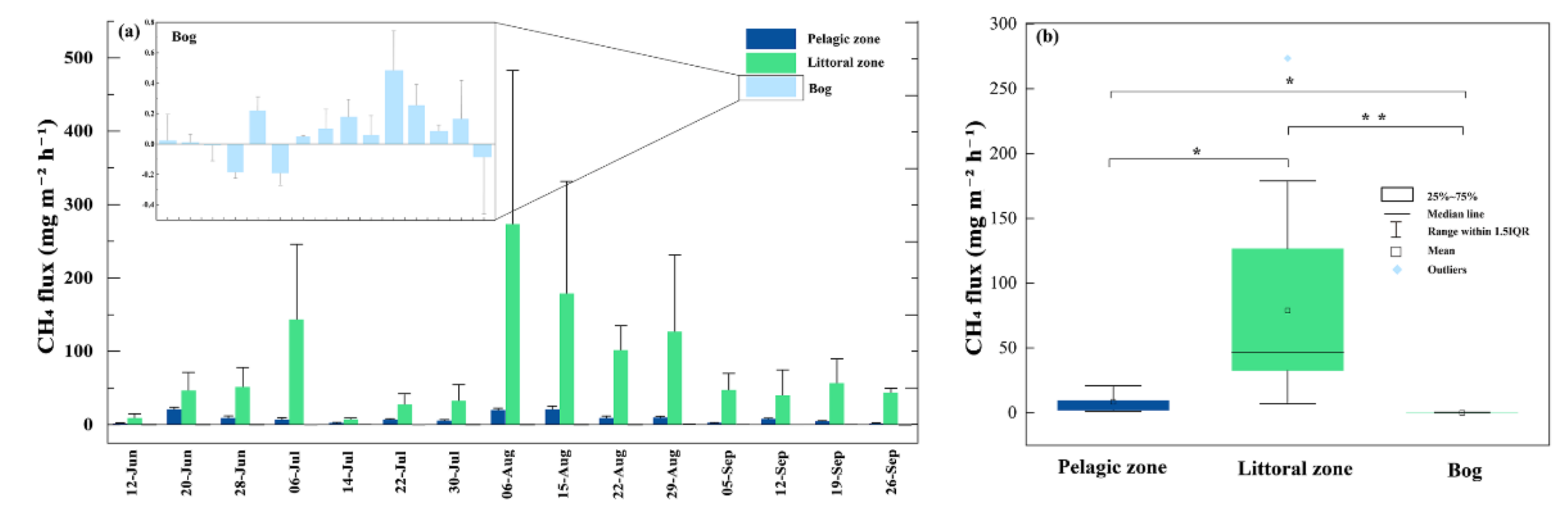
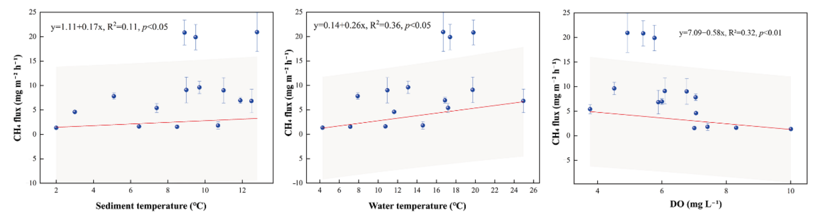
On the temporal scale, CH4 fluxes were highest in August at all three sites, but the lowest fluxes occurred at different periods. In the pelagic zone, the lowest flux value occurred in September with a value of 1.35 mg m−2 h−1. In the littoral zone and bog, the lowest flux occurred in July with values of 7.02 mg m−2 h−1 and −0.19 mg m−2 h−1, respectively (Figure 2a). On the scale of spatial scale, CH4 fluxes were highest in the littoral zone, with fluxes two–three orders of magnitude greater than those from the adjacent bog (Figure 2b). The average flux in the littoral zone was 78.98 ± 19.00 mg m−2 h−1. The mean fluxes at the other two sites were 8.48 ± 1.77 mg m−2 h−1 in the pelagic zone and 0.07 ± 0.05 mg m−2 h−1 in the bog, respectively. CH4 fluxes were significantly different in these three sample sites (p < 0.01, Figure 2b). CH4 fluxes in the pond were positively correlated with sediment temperature (p < 0.05, Figure 3) and water temperature (p < 0.05, Figure 3) and negatively correlated with dissolved oxygen (p < 0.01, Figure 3).
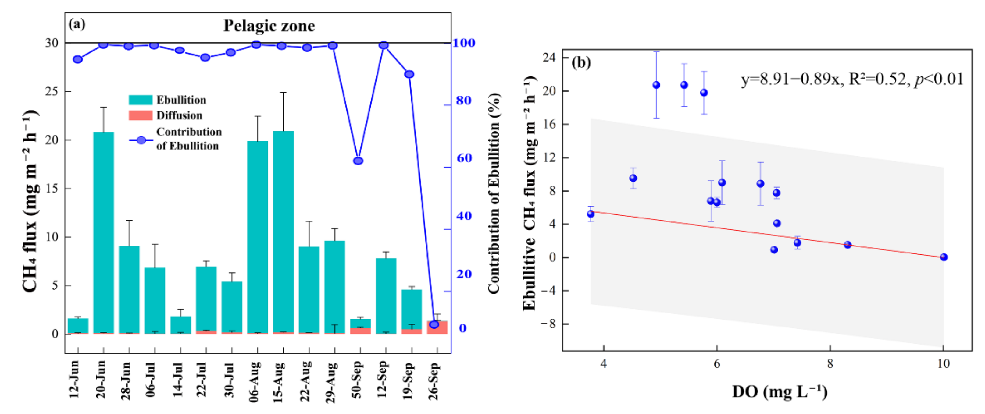
Within the pond, the highest CH4 ebullition fluxes occurred in August while the highest diffusive fluxes both occurred in late September. On average, ebullition accounted for 88.56% of the total CH4 fluxes in the pelagic zone (Figure 4a). Ebullition dominated the CH4 fluxes and was negatively correlated with DO (p < 0.01) (Figure 4b).
3.3. CO2 Fluxes
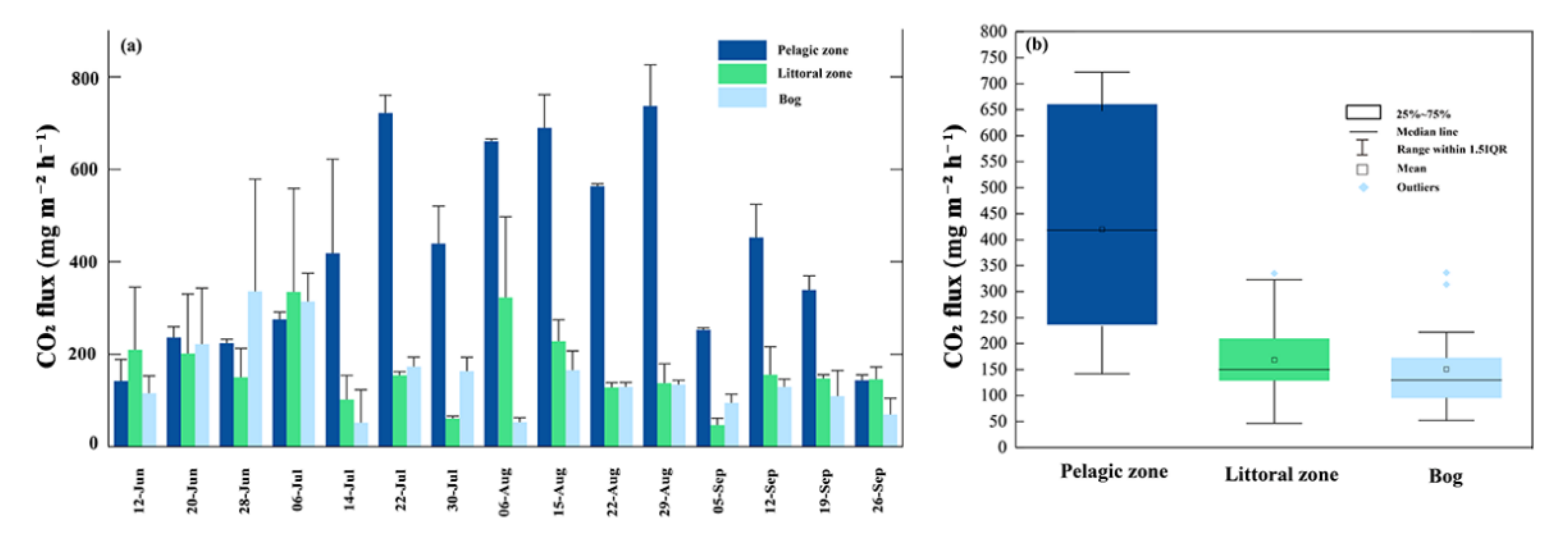
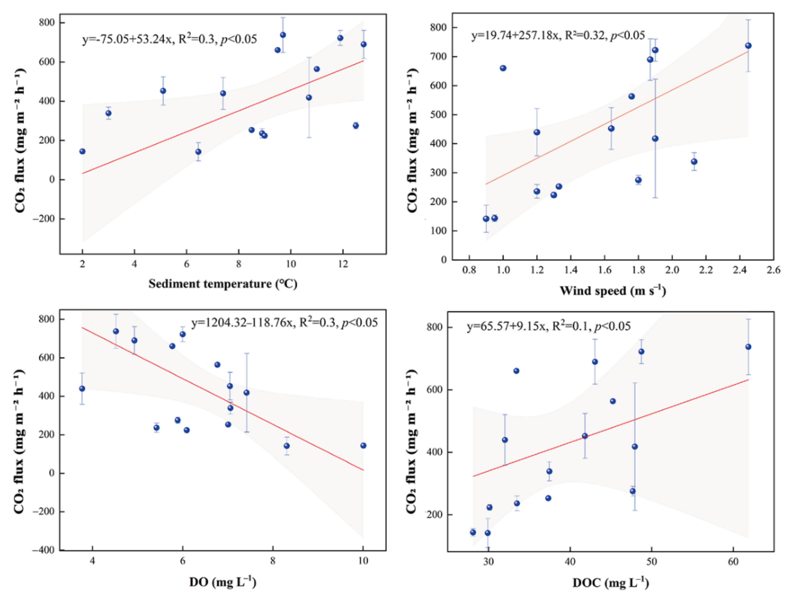
On the temporal scale, CO2 fluxes showed a general trend of increasing and then decreasing over time in the pelagic zone, with higher fluxes in July/August. In the littoral zone, the maximum CO2 fluxes occur in July (Figure 5a). In the bog, peak CO2 fluxes occurred early in the growing season. The mean values for the three sites were 419.76 mg m−2 h−1, 168.41 mg m−2 h−1 and 150.72 mg m−2 h−1, respectively. CO2 fluxes in the pelagic zone were positively correlated with sediment temperature (p < 0.05, Figure 6), wind speed (p < 0.05, Figure 6) and dissolved organic carbon (p < 0.05, Figure 6) and negatively correlated with dissolved oxygen (p < 0.05, Figure 6).
3.4. N2O Fluxes
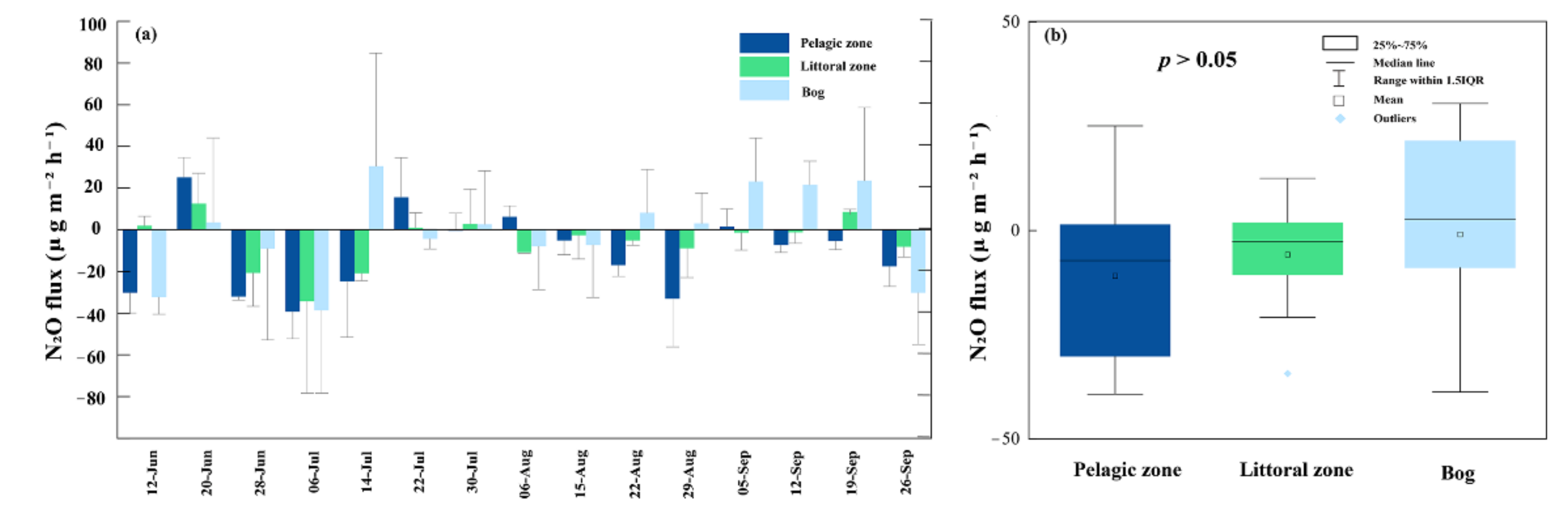
N2O fluxes ranged from −39.22–25.12 μg m−2 h−1, −34.31–12.56 μg m−2 h−1 and −38.73–30.50 μg m−2 h−1 in the pelagic zone, littoral zone and bog, respectively (Figure 7a); their minimum values occur in July. The mean fluxes of N2O at the three sites as sinks were −10.90 μg m−2 h−1, −5.80 μg m−2 h−1 and −0.90 μg m−2 h−1, respectively. There were no significant differences among these three sites fluxes (p = 0.425, Figure 7b). In all sites, N2O fluxes did not correlate with any observed environmental factors (p > 0.05).
4. Discussion
4.1. CH4 Fluxes
4.1.1. CH4 Fluxes within the Pond
The studied peatland pond was a net source of CH4 throughout the growing season, with ebullition being the main way of emissions. Compared to other boreal peatland ponds, the pond in our study had higher fluxes than ponds in Canada [38]. This may be because of the fact that the area we studied was in a permafrost zone, where melting permafrost increases carbon emissions. In contrast, the CH4 fluxes from thermokarst lakes in the Qinghai-Tibet Plateau, which is also located in the permafrost zone, is two times higher than in our study [39]. Carbon release rates may be higher in thermokarst lakes formed due to permafrost thawing. Nutrient cycling rates within small ponds are rapid [40], and CH4 emission rates are usually higher than those in larger lakes. The CH4 flux rate in our pond was higher than that reported in large lakes in Finland [41].
Within the pond, ebullition accounted for over 80% of the total CH4 fluxes. The high fluxes of ebullition occurred in August, with the lowest values occurring in June and September, which was consistent with previous studies [37,42]. Seasonal patterns of CH4 emissions are temperature dependent. CH4 production and emissions increase with temperature [43]. This is also indicated by the positive correlation between CH4 fluxes and water or sediment temperatures (Figure 4). Increased temperature stimulated the activity of methanogenic bacteria and accelerated CH4 production rates [44]. Thus, in the month with high temperatures, CH4 fluxes increased. Small, shallow ponds tended to have high ebullition fluxes [45,46,47]. The shallower water column compared to large lakes limits the time that CH4 bubbles can remain in the oxygenated water column, reducing the oxidation of CH4 in the bubbles [13,48]. Ebullition fluxes were negatively correlated with DO in our study (Figure 5), which is consistent with previous studies [8]. Furthermore, we analyzed the relationship between ebullition flux and air pressure but did not find a correlation between them. Although air pressure can be proved to facilitate the release of bubbles from sediments [49,50].
4.1.2. The Littoral Zone Was a Hotspot for CH4 Fluxes Compared to Pond and Adjacent Bog
Our results showed a large spatial variation in CH4 emissions, with the littoral zone making a significant contribution to pond CH4 emissions. Also in boreal regions, higher CH4 emissions from the littoral than from the pelagic zones of shallow lakes have been reported [46,51]. In our study, the littoral zone was an ecotone between the pond and adjacent bog, with CH4 emissions three magnitudes higher than the adjacent bog and one magnitude higher than the pelagic zone (Figure 2b). The extremely high CH4 emissions in the littoral zone were driven by both biological and abiotic factors. The rich organic matter in the littoral zone provides more substrate for methanogens and promotes CH4 production [52,53]. Previous studies on boreal lakes have shown that vegetation-mediated CH4 emissions from the littoral zone can account for 60–80% of CH4 emissions from the lake [28]. The CH4 transport rates depend on the plant species; commonly, Carex-dominated vegetation types have greater CH4 flux rates than other plants [54]. There was a significant spread of Carex species in the littoral zone, which can transport CH4 through the aerenchyma and bypass the oxygen layer [55,56,57]. The CH4 fluxes in the bog were much lower than those in the littoral zone. This is because the bog was dominated by shrubs and trees, which do not have well-developed aerenchyma to facilitate CH4 transport. Sphagnum was widely distributed in the bog, and the microbes on and within it could oxidize CH4 and further reduce its emissions [58,59]. In addition, the bog had the lowest water level of all the studied sites, which was one of the reasons that the bog was a very small source of CH4 emissions. Temperature is an important factor influencing soil CH4 fluxes. CH4 flux peaks were also tending to occur during the period when soil temperatures were high in August (Figure 2a). High temperatures can promote both methanogenesis from methanogens and CH4 oxidation from methanotrophs; CH4 fluxes depend on the balance of these two processes [60]. The negative CH4 fluxes that occurred in the bog during periods of high temperature (Figure 2a) indicated that CH4 oxidation was dominant at this time.
4.2. CO2 Fluxes
Temporal and spatial variation in the pond was related to a variety of environmental factors such as temperature, DOC or rainfall events. Sediment organic carbon mineralization was strongly dependent on temperature. As sediment temperature increases, organic carbon burial efficiency decreases, leading to enhanced CO2 emissions from the lake [61,62]. Thus, when sediment temperature was the highest in August, CO2 fluxes in the pelagic zone also reach a maximum during this period. CO2 fluxes in pelagic zone were lower in June and September. This is due to the low water temperature during this time, which reduces the production of CO2 by microorganisms through respiration [63]. The factor driving the temporal variability of CO2 fluxes in the ponds was DOC, as indicated by the positive correlation between CO2 fluxes and DOC in the pelagic zone (p < 0.05). DOC is an important source of carbon for aquatic ecosystems [64] and has a significant impact on CO2 emissions [65,66,67]. Peatland ponds can be a source of CO2 through several pathways: sediment respiration, oxidation of CH4 [30] sunlight-induced photochemical mineralization of colored dissolved organic matter (CDOM) [68] and inflowing streams and littoral areas providing dissolved gases [69]. The peatland pond we studied was strongly controlled by hydrological events. Hydrological inputs to the pond were from the bog and large amounts of precipitation during the growing season. Precipitation not only dilutes chemical parameters in the pond, but also controls DOC flow and diffusion, possibly providing the pond with dissolved gases and contributing to the high CO2 fluxes in the pond. Precipitation brought DOC from the bog into the littoral zone and increased DOC supply leads to higher CO2 fluxes at this time.
Previous studies have reported on spatial patterns of CO2 fluxes in shallow lakes [70]. This spatial heterogeneity is associated with differences between pelagic and littoral zone [71]. CO2 in the pond mainly came from sediment respiration [64]. Sediment respiration consumes oxygen to produce CO2, and high sediment temperature also facilitates CO2 emissions. The pelagic zone showed a negative correlation with DO (p < 0.05) and a positive correlation with sediment temperature (p < 0.05), indicating that sediment respiration was strongest in this zone, which may lead to higher CO2 fluxes. Wind speed can influence CO2 fluxes by controlling the rate of gas transport at the water-air interface [72]. The open water of the pelagic zone was susceptible to wind, thus enhancing pond turbulence in the pelagic zone and stimulating the escape of CO2 from the pelagic zone into the atmosphere. The positive correlation between CO2 fluxes and wind speed in the pelagic zone (p < 0.01) showed the effect of wind on CO2 fluxes and indicated that diffusion was the pathway for CO2 emissions in our study.
Small shallow peatland ponds are a powerful source of atmospheric CO2. The sediment decomposition of these ponds is greater than in large deep lakes [38]. Sediment with high carbon content is the characteristic of peatland ponds, which is an important source of carbon emissions from northern ponds or lakes [66]. The pond we studied had three times more CO2 fluxes than Canadian peatland ponds [46]. High CO2 emission fluxes may be common feedback from permafrost peatlands to climate change. Typically, small ponds tend to have higher average CO2 emission rates than larger and deeper lakes. Compared to the large lakes in Finland [41], the CO2 emissions in this study are more than 20 times higher than in their study. Lake types and the hydrological conditions help us to understand the differences in lakes/ponds’ CO2 emissions.
4.3. N2O Fluxes
There was no significant spatial variation in N2O fluxes (p > 0.05). On the time scale, all sites alternated between sources and sinks but mainly showed as a sink. This may depend on the relative rates of N2O production and consumption at any particular time [73]. N2O flux peaks from water bodies usually occur in winter, and the lowest values of N2O fluxes occur during the open water season when lakes are likely to behave as a sink [74]. On the spatial scale, both pelagic zone, littoral zone and adjacent bog exhibited sinks for N2O fluxes. Small water bodies can be sinks for N2O, which has also been demonstrated in previous studies [15,75]. This is related to the availability of organic carbon and oxygen in the water column and the stratification of the water column. N2O is produced mainly through nitrification and denitrification by microorganisms; denitrification is usually predominant in aquatic ecosystems [76]. N2O can be produced at the boundary of the hypoxic layer of the water column due to the denitrification process, which demands an appropriate anoxic environment for N2O production. However, N2O is rapidly exhausted under extreme anoxic conditions, which explains the unsaturation of N2O in the completely anoxic layer [77]. The sediment contained an extremely low level of oxygen and provided a completely anoxic environment. Therefore, N2O was consumed at the bottom of the pond. The concentration gradient resulting from the unsaturation of N2O in the completely anoxic layer may be one of the reasons for the uptake of N2O by the water body. Another reason for N2O uptake in the pond we studied was related to organic carbon availability. When the C source is restricted, denitrification cannot proceed completely [78], resulting in the production of the intermediate product N2O. The high DOC (>20 mg L−1) concentration regulates the rate of denitrification and facilitates N2O consumption [15]. This explains the pond we studied as a sink in the landscape because of the very high DOC level in the water of the pond (average 39.88 mg L−1, Table S1). Similarly, organic carbon input from the abundance of plants in the bog and littoral fringe provides energy for denitrifying bacteria, with N2 being the main product after complete denitrification [78]. Our results suggest that the peatland pond and adjacent bog in the boreal region are not a significant source of atmospheric N2O. The average N2O fluxes in the pond in the study area were −6.6 μg m−2 h−1, which was lower than the pond in Finland (−0.26 μg m−2 h−1) [79]. They both showed as sinks for N2O. Anthropogenic inputs of nitrogen and phosphorus are the main reasons for the high N2O fluxes from some lakes, which have much larger N2O fluxes than the pond we studied [27,80,81]. However, due to the effects of global warming, there is a trend toward N2O emissions from ponds and peatlands in boreal regions because of permafrost thawing [35]. Therefore, longer timescale observations are needed for changes in ponds N2O fluxes in the study area, as the permafrost in this region is thawing [31].
4.4. Implications for the Peatland Pond System from Peatland Landscapes
Peatland ecosystems are widely distributed in boreal landscapes [14]. They can provide critical information on the terrestrial carbon cycle [66]. Permafrost thawing may have exacerbated the transport of carbon from the peatland to aquatic systems [25]. These aquatic systems can act as conduits for the transport to the atmosphere of carbon immobilized in terrestrial ecosystems [82]. Warming leads to an expansion in the number and size of boreal lakes [83], this may convert a part of the peatland into a permanent aquatic system. Our results suggest that the peatland pond and its littoral zones were a large source of carbon emissions. Uncertainties in lake CH4 flux estimation include the lack of data in the littoral zone, and an accurate assessment of CH4 fluxes in the littoral zone requires our attention. Future studies could quantify the GHG balance in peatland landscapes and aquatic systems in this region, which would help to understand the importance of these aquatic systems in regional GHG emissions.
5. Conclusions
The spatiotemporal variation of GHG emissions from a pond and adjacent bog was studied. Within the pond, ebullition was the main pathway for CH4 emissions, accounting for over 80% of the total fluxes, and the littoral zone was a hotspot for CH4 emissions. CO2 was emitted mainly through diffusion, and the hotspot was the pelagic zone. Therefore, using only a diffusion-based model (as in Equation (2)) dependent on the gas concentration deficit between the air and water will underestimate CH4 fluxes in ponds with high ebullition rates. Environmental factors such as DO, DOC and wind speed significantly predict pond carbon gas emissions. Overall, although the peatland pond was an important source of CH4 and CO2 emissions, it can act as a sink for N2O.
Supplementary Materials
The following supporting information can be downloaded at: https://www.mdpi.com/article/10.3390/w15020307/s1, Table S1: Hydrochemical parameter data in the water column in pelagic zone of the pond.
Author Contributions
Conceptualization, J.X. and X.S.; methodology, X.S.; investigation, J.X. and X.C.; data curation, X.C. and X.W.; writing—original draft preparation, J.X., X.C. and X.S.; visualization, X.W., X.C. and X.S.; project administration, X.S.; funding acquisition, X.S. All authors have read and agreed to the published version of the manuscript.
Funding
This research was supported by the Fundamental Research Funds for the Central Universities (grant number 2572020BA06; 2572021DS04); the National Natural Science Foundation of China (grant number 31870443).
Data Availability Statement
The datasets generated during the current study are available from the corresponding author on reasonable request.
Acknowledgments
The authors appreciate the anonymous reviewers for their constructive comments and suggestions that significantly improved the quality of this manuscript.
Conflicts of Interest
The authors declare no conflict of interest.
References
- IPCC, Intergovernmental Panel on Climate Change. The Physical Science Basis; Contribution of Working Group I to the Sixth Assessment Report of the Intergovernmental Panel on Climate Change; Masson-Delmotte, V.P., Zhai, A., Pirani, S.L., Connors, C., Péan, S., Berger, N., Caud, Y., Chen, L., Goldfarb, M.I., Gomis, M., et al., Eds.; Cambridge University Press: Cambridge, UK, 2021. (in press) [Google Scholar]
- World Meteorological Organization (WMO). WMO Greenhouse Gas Bulletin (GHG Bulletin)—No. 15: The State of Greenhouse Gases in the Atmosphere Based on Global Observations through 2018; WHO: Geneva, Switzerland, 2019; Available online: https://library.wmo.int/index.php?lvl=notice_display&id=21620 (accessed on 1 January 2021).
- Verpoorter, C.; Kutser, T.; Seekell, D.A.; Tranvik, L.J. A global inventory of lakes based on high-resolution satellite imagery. Geophys. Res. Lett. 2014, 41, 6396–6402. [Google Scholar] [CrossRef]
- Raymond, P.; Hartmann, J.; Lauerwald, R.; Sobek, S.; McDonald, C.; Hoover, M.; Butman, D.; Striegl, R.; Mayorga, E.; Humborg, C.; et al. Global carbon dioxide emissions from inland waters. Nature 2013, 503, 355–359. [Google Scholar] [CrossRef] [Green Version]
- DelSontro, T.; Beaulieu, J.; Downing, J. Greenhouse gas emissions from lakes and impoundments: Upscaling in the face of global change. Limnol. Oceanogr. Lett. 2018, 3, 64–75. [Google Scholar] [CrossRef]
- Rosentreter, J.A.; Borges, A.V.; Deemer, B.R.; Holgerson, M.A.; Liu, S.; Song, C.; Melack, J.; Raymond, P.A.; Duarte, C.M.; Allen, G.H.; et al. Half of global methane emissions come from highly variable aquatic ecosystem sources. Nat. Geosci. 2021, 14, 225–230. [Google Scholar] [CrossRef]
- Cole, J.J.; Prairie, Y.T.; Caraco, N.F.; McDowell, W.H.; Tranvik, L.J.; Striegl, R.G.; Duarte, C.M.; Kortelainen, P.; Downing, J.A.; Middelburg, J.J.; et al. Plumbing the global carbon cycle: Integrating inland waters into the terrestrial carbon budget. Ecosystems 2007, 10, 172–185. [Google Scholar] [CrossRef] [Green Version]
- Holgerson, M.A.; Raymond, P.A. Large contribution to inland water CO2 and CH4 emissions from very small ponds. Nat. Geosci. 2016, 9, 222–226. [Google Scholar] [CrossRef]
- Martinsen, K.T.; Kragh, T.; Sand-Jensen, K. Carbon dioxide efflux and ecosystem metabolism of small forest lakes. Aquat. Sci. 2019, 82, 9. [Google Scholar] [CrossRef]
- Woolway, R.I.; Kraemer, B.M.; Lenters, J.D.; Merchant, C.J.; O’Reilly, C.M.; Sharma, S. Global lake responses to climate change. Nat. Rev. Earth Environ. 2020, 1, 388–403. [Google Scholar] [CrossRef]
- Tranvik, L.J.; Downing, J.A.; Cotner, J.B.; Loiselle, S.A.; Striegl, R.G.; Ballatore, T.J.; Dillon, P.; Finlay, K.; Fortino, K.; Knoll, L.B.; et al. Lakes and reservoirs as regulators of carbon cycling and climate. Limnol. Oceanogr. 2009, 54, 2298–2314. [Google Scholar] [CrossRef] [Green Version]
- Huttunen, J.T.; Alm, J.; Liikanen, A.; Juutinen, S.; Larmola, T.; Hammar, T.; Silvola, J.; Martikainen, P.J. Fluxes of methane, carbon dioxide and nitrous oxide in boreal lakes and potential anthropogenic effects on the aquatic greenhouse gas emissions. Chemosphere 2003, 52, 609–621. [Google Scholar] [CrossRef] [PubMed]
- Bastviken, D.; Cole, J.J.; Pace, M.L.; Van de Bogert, M.C. Fates of methane from different lake habitats: Connecting whole-lake budgets and CH4 emissions. J. Geophys. Res. Biogeosci. 2008, 113(G2), 61–74. [Google Scholar] [CrossRef]
- Kortelainen, P.; Larmola, T.; Rantakari, M.; Juutinen, S.; Alm, J.; Martikainen, P.J. Lakes as nitrous oxide sources in the boreal landscape. Glob. Change Biol. 2020, 26, 1432–1445. [Google Scholar] [CrossRef] [PubMed] [Green Version]
- Soued, C.; del Giorgio, P.A.; Maranger, R. Nitrous oxide sinks and emissions in boreal aquatic networks in Québec. Nat. Geosci. 2016, 9, 116–120. [Google Scholar] [CrossRef]
- Cole, J.; Caraco, N. Atmospheric exchange of carbon dioxide in a low-wind oligotrophic lake measured by the addition of SF6. Limnol. Oceanogr. 1998, 43, 647–656. [Google Scholar] [CrossRef] [Green Version]
- Gao, Y.; Liu, X.; Yi, N.; Wang, Y.; Guo, J.; Zhang, Z.; Yan, S. Estimation of N2 and N2O ebullition from eutrophic water using an improved bubble trap device. Ecol. Eng. 2013, 57, 403–412. [Google Scholar] [CrossRef] [Green Version]
- Sepulveda-Jauregui, A.; Walter Anthony, K.; Martinez-Cruz, K.; Greene, S.; Thalasso, F. Methane and carbon dioxide emissions from 40 lakes along a north–south latitudinal transect in Alaska. Biogeosciences 2015, 12, 3197–3223. [Google Scholar] [CrossRef] [Green Version]
- Bastviken, D.; Cole, J.; Pace, M.; Tranvik, L. Methane emissions from lakes: Dependence of lake characteristics, two regional assessments, and a global estimate. Glob. Biogeochem. Cycles 2004, 18. [Google Scholar] [CrossRef]
- Li, M.; Peng, C.; Zhu, Q.; Zhou, X.; Yang, G.; Song, X.; Zhang, K. The significant contribution of lake depth in regulating global lake diffusive methane emissions. Water Res. 2020, 172, 115465. [Google Scholar] [CrossRef]
- Baulch, H.M.; Dillon, P.J.; Maranger, R.; Schiff, S.L. Diffusive and ebullitive transport of methane and nitrous oxide from streams: Are bubble-mediated fluxes important? J. Geophys. Res. Biogeosci. 2011, 116. [Google Scholar] [CrossRef]
- Saunois, M.; Bousquet, P.; Poulter, B.; Peregon, A.; Ciais, P.; Canadell, J.; Dlugokencky, E.; Etiope, G.; Bastviken, D.; Houweling, S.; et al. The global methane budget 2000–2012. Earth Syst. Sci. Data 2016, 8, 697–751. [Google Scholar] [CrossRef]
- Desrosiers, K.; DelSontro, T.; del Giorgio, P.A. Disproportionate contribution of vegetated habitats to the CH4 and CO2 budgets of a boreal lake. Ecosystems 2022, 25, 1522–1541. [Google Scholar] [CrossRef]
- Woodman, S.G.; Khoury, S.; Fournier, R.E.; Emilson, E.J.S.; Gunn, J.M.; Rusak, J.A.; Tanentzap, A.J. Forest defoliator outbreaks alter nutrient cycling in northern waters. Nat. Commun. 2021, 12, 6355. [Google Scholar] [CrossRef]
- Tanentzap, A.J.; Burd, K.; Kuhn, M.; Estop-Aragonés, C.; Tank, S.E.; Olefeldt, D. Aged soils contribute little to contemporary carbon cycling downstream of thawing permafrost peatlands. Glob. Change Biol. 2021, 27, 5368–5382. [Google Scholar] [CrossRef]
- Groffman, P.; Gold, A.; Addy, K. Nitrous oxide production in riparian zones and its importance to national emission inventories. Chemosphere—Glob. Change Sci. 2000, 2, 291–299. [Google Scholar] [CrossRef]
- Wang, H.; Wang, W.; Yin, C.; Wang, Y.; Lu, J. Littoral zones as the “hotspots” of nitrous oxide (N2O) emission in a hyper-eutrophic lake in China. Atmos. Environ. 2006, 40, 5522–5527. [Google Scholar] [CrossRef]
- Vesterinen, J.; Devlin, S.P.; Syväranta, J.; Jones, R.I. Influence of littoral periphyton on whole-lake metabolism relates to littoral vegetation in humic lakes. Ecology 2017, 98, 3074–3085. [Google Scholar] [CrossRef] [Green Version]
- Juutinen, S.; Alm, J.; Larmola, T.; Huttunen, J.T.; Morero, M.; Martikainen, P.J.; Silvola, J. Major implication of the littoral zone for methane release from boreal lakes. Glob. Biogeochem. Cycles 2003, 17. [Google Scholar] [CrossRef]
- Kankaala, P.; Huotari, J.; Tulonen, T.; Ojala, A. Lake-size dependent physical forcing drives carbon dioxide and methane effluxes from lakes in a boreal landscape. Limnol. Oceanogr. 2013, 58, 1915–1930. [Google Scholar] [CrossRef]
- Sun, X.; Wang, H.; Song, C.; Jin, X.; Richardson, C.; Cai, T. Response of methane and nitrous oxide emissions from peatlands to permafrost thawing in Xiaoxing’an Mountains, Northeast China. Atmosphere 2021, 12, 222. [Google Scholar] [CrossRef]
- Guo, Y.; Song, C.; Wang, L.; Tan, W.; Wang, X.; Cui, Q.; Wan, Z. Concentrations, sources, and export of dissolved CH4 and CO2 in rivers of the permafrost wetlands, northeast China. Ecol. Eng. 2016, 90, 491–497. [Google Scholar] [CrossRef]
- Wiesenburg, D.; Guinasso, N. Equilibrium solubilities of methane, carbon monoxide, and hydrogen in water and sea water. J. Chem. Eng. Data 2002, 24, 356. [Google Scholar] [CrossRef]
- Wanninkhof, R. Relationship between wind speed and gas exchange over the ocean. J. Geophys. Res. Ocean. 1992, 97, 7373–7382. [Google Scholar] [CrossRef]
- Yan, F.; Sillanpää, M.; Kang, S.; Aho, K.; Qu, B.; Wei, D.; Li, X.; Li, C.; Raymond, P. Lakes on the Tibetan Plateau as conduits of greenhouse gases to the atmosphere. J. Geophys. Res. Biogeosci. 2018, 123, 2091–2103. [Google Scholar] [CrossRef]
- Zhang, L.; Xia, X.; Liu, S.; Zhang, S.; Li, S.; Wang, J.; Wang, G.; Gao, H.; Zhang, Z.; Wang, Q.; et al. Significant methane ebullition from alpine permafrost rivers on the East Qinghai–Tibet Plateau. Nat. Geosci. 2020, 13, 1–6. [Google Scholar] [CrossRef]
- Wang, L.; Du, Z.; Wei, Z.; Xu, Q.; Feng, Y.; Lin, P.; Lin, J.; Chen, S.; Qiao, Y.; Shi, J.; et al. High methane emissions from thermokarst lakes on the Tibetan Plateau are largely attributed to ebullition fluxes. Sci. Total Environ. 2021, 801, 149692. [Google Scholar] [CrossRef] [PubMed]
- McEnroe, N.A.; Roulet, N.T.; Moore, T.R.; Garneau, M. Do pool surface area and depth control CO2 and CH4 fluxes from an ombrotrophic raised bog, James Bay, Canada? J. Geophys. Res. Biogeosci. 2009, 114. [Google Scholar] [CrossRef] [Green Version]
- Zhu, D.; Wu, Y.; Chen, H.; He, Y.; Wu, N. Intense methane ebullition from open water area of a shallow peatland lake on the eastern Tibetan Plateau. Sci. Total Environ. 2016, 542, 57–64. [Google Scholar] [CrossRef]
- Wetzel, R.G. Limnology: Lake and River Ecosystems, 3rd ed.; Academic Press: San Diego, CA, USA, 2001; p. 1006. [Google Scholar]
- Ojala, A.; Bellido, J.L.; Tulonen, T.; Kankaala, P.; Huotari, J. Carbon gas fluxes from a brown-water and a clear-water lake in the boreal zone during a summer with extreme rain events. Limnol. Oceanogr. 2011, 56, 61–76. [Google Scholar] [CrossRef]
- Wik, M.; Crill, P.M.; Varner, R.K.; Bastviken, D. Multiyear measurements of ebullitive methane flux from three subarctic lakes. J. Geophys. Res. Biogeosci. 2013, 118, 1307–1321. [Google Scholar] [CrossRef] [Green Version]
- Yvon-Durocher, G.; Allen, A.P.; Bastviken, D.; Conrad, R.; Gudasz, C.; St-Pierre, A.; Thanh-Duc, N.; del Giorgio, P.A. Methane fluxes show consistent temperature dependence across microbial to ecosystem scales. Nature 2014, 507, 488–491. [Google Scholar] [CrossRef] [PubMed]
- Duc, N.T.; Crill, P.; Bastviken, D. Implications of temperature and sediment characteristics on methane formation and oxidation in lake sediments. Biogeochemistry 2010, 100, 185–196. [Google Scholar] [CrossRef]
- Natchimuthu, S.; Panneer Selvam, B.; Bastviken, D. Influence of weather variables on methane and carbon dioxide flux from a shallow pond. Biogeochemistry 2014, 119, 403–413. [Google Scholar] [CrossRef]
- Burger, M.; Berger, S.; Spangenberg, I.; Blodau, C. Summer fluxes of methane and carbon dioxide from a pond and floating mat in a continental Canadian peatland. Biogeosciences 2016, 13, 3777–3791. [Google Scholar] [CrossRef] [Green Version]
- Baron, A.A.P.; Dyck, L.T.; Amjad, H.; Bragg, J.; Kroft, E.; Newson, J.; Oleson, K.; Casson, N.J.; North, R.L.; Venkiteswaran, J.J.; et al. Differences in ebullitive methane release from small, shallow ponds present challenges for scaling. Sci. Total Environ. 2022, 802, 149685. [Google Scholar] [CrossRef] [PubMed]
- Peacock, M.; Audet, J.; Bastviken, D.; Cook, S.; Evans, C.D.; Grinham, A.; Holgerson, M.A.; Högbom, L.; Pickard, A.E.; Zieliński, P.; et al. Small artificial waterbodies are widespread and persistent emitters of methane and carbon dioxide. Glob. Change Biol. 2021, 27, 5109–5123. [Google Scholar] [CrossRef]
- Casper, P.; Maberly, S.C.; Hall, G.H.; Finlay, B.J. Fluxes of methane and carbon dioxide from a small productive lake to the atmosphere. Biogeochemistry 2000, 49, 1–19. [Google Scholar] [CrossRef]
- Boereboom, T.; Depoorter, M.; Coppens, S.; Tison, J.-L. Gas properties of winter lake ice in Northern Sweden. Biogeosci. Discuss. 2011, 9, 827–838. [Google Scholar] [CrossRef] [Green Version]
- Hofmann, H. Spatiotemporal distribution patterns of dissolved methane in lakes: How accurate are the current estimations of the diffusive flux path? Geophys. Res. Lett. 2013, 40, 2779–2784. [Google Scholar] [CrossRef]
- Bergman, I.; Klarqvist, M.; Nilsson, M. Seasonal variation in rates of methane production from peat of various botanical origins. FEMS Microbiol. Ecol. 2000, 33, 181–189. [Google Scholar] [CrossRef] [PubMed]
- Singh, S.N.; Kulshreshtha, K.; Agnihotri, S. Seasonal dynamics of methane emission from wetlands. Chemosphere—Glob. Change Sci. 2000, 2, 39–46. [Google Scholar] [CrossRef]
- Korrensalo, A.; Mammarella, I.; Alekseychik, P.; Vesala, T.; Tuittila, E.S. Plant mediated methane efflux from a boreal peatland complex. Plant Soil 2021, 471, 375–392. [Google Scholar] [CrossRef]
- Sun, X.; Song, C.; Guo, Y.; Wang, X.; Yang, G.; Li, Y.; Mao, R.; Yongzheng, L. Effect of plants on methane emissions from a temperate marsh in different seasons. Atmos. Environ. 2012, 60, 277–282. [Google Scholar] [CrossRef]
- Turner, J.C.; Moorberg, C.J.; Wong, A.; Shea, K.; Waldrop, M.P.; Turetsky, M.R.; Neumann, R.B. Getting to the root of plant-mediated methane emissions and oxidation in a thermokarst bog. J. Geophys. Res. Biogeosci. 2020, 125, e2020JG005825. [Google Scholar] [CrossRef]
- Kao-Kniffin, J.; Freyre, D.S.; Balser, T.C. Methane dynamics across wetland plant species. Aquat. Bot. 2010, 93, 107–113. [Google Scholar] [CrossRef]
- Raghoebarsing, A.A.; Smolders, A.J.P.; Schmid, M.C.; Rijpstra, W.I.C.; Wolters-Arts, M.; Derksen, J.; Jetten, M.S.M.; Schouten, S.; Sinninghe Damsté, J.S.; Lamers, L.P.M.; et al. Methanotrophic symbionts provide carbon for photosynthesis in peat bogs. Nature 2005, 436, 1153–1156. [Google Scholar] [CrossRef] [PubMed] [Green Version]
- Kip, N.; van Winden, J.F.; Pan, Y.; Bodrossy, L.; Reichart, G.-J.; Smolders, A.J.P.; Jetten, M.S.M.; Damsté, J.S.S.; Op den Camp, H.J.M. Global prevalence of methane oxidation by symbiotic bacteria in peat-moss ecosystems. Nat. Geosci. 2010, 3, 617–621. [Google Scholar] [CrossRef]
- Winden, J.; Reichart, G.-J.; McNamara, N.; Benthien, A.; Sinninghe-Damste, J. Temperature-induced increase in methane release from peat bogs: A mesocosm experiment. PLoS ONE 2012, 7, e39614. [Google Scholar] [CrossRef] [Green Version]
- Gudasz, C.; Bastviken, D.; Steger, K.; Premke, K.; Sobek, S.; Tranvik, L.J. Temperature-controlled organic carbon mineralization in lake sediments. Nature 2010, 466, 478–481. [Google Scholar] [CrossRef] [PubMed] [Green Version]
- Marotta, H.; Pinho, L.; Gudasz, C.; Bastviken, D.; Tranvik, L.J.; Enrich-Prast, A. Greenhouse gas production in low-latitude lake sediments responds strongly to warming. Nat. Clim. Change 2014, 4, 467–470. [Google Scholar] [CrossRef]
- Åberg, J.; Jansson, M.; Jonsson, A. Importance of water temperature and thermal stratification dynamics for temporal variation of surface water CO2 in a boreal lake. J. Geophys. Res. Biogeosci. 2010, 115. [Google Scholar] [CrossRef]
- Rantakari, M.; Kortelainen, P. Interannual variation and climatic regulation of the CO2 emission from large boreal lakes. Glob. Change Biol. 2005, 11, 1368–1380. [Google Scholar] [CrossRef]
- Ask, J.; Karlsson, J.; Jansson, M. Net ecosystem production in clear-water and brown-water lakes. Glob. Biogeochem. Cycles 2012, 26. [Google Scholar] [CrossRef]
- Shirokova, L.S.; Payandi-Rolland, D.; Lim, A.G.; Manasypov, R.M.; Allen, J.; Rols, J.L.; Bénézeth, P.; Karlsson, J.; Pokrovsky, O.S. Diel cycles of carbon, nutrient and metal in humic lakes of permafrost peatlands. Sci. Total Environ. 2020, 737, 139671. [Google Scholar] [CrossRef] [PubMed]
- Jongejans, L.; Liebner, S.; Knoblauch, C.; Mangelsdorf, K.; Ulrich, M.; Grosse, G.; Tanski, G.; Fedorov, A.; Konstantinov, P.; Windirsch, T.; et al. Greenhouse gas production and lipid biomarker distribution in Yedoma and Alas thermokarst lake sediments in Eastern Siberia. Glob. Change Biol. 2021, 27, 2822–2839. [Google Scholar] [CrossRef] [PubMed]
- Groeneveld, M.; Tranvik, L.; Natchimuthu, S.; Koehler, B. Photochemical mineralisation in a boreal brown water lake: Considerable temporal variability and minor contribution to carbon dioxide production. Biogeosciences 2016, 13, 3931–3943. [Google Scholar] [CrossRef] [Green Version]
- Juutinen, S.; Väliranta, M.; Kuutti, V.; Laine, A.M.; Virtanen, T.; Seppä, H.; Weckström, J.; Tuittila, E.S. Short-term and long-term carbon dynamics in a northern peatland-stream-lake continuum: A catchment approach. J. Geophys. Res. Biogeosci. 2013, 118, 171–183. [Google Scholar] [CrossRef]
- Xiao, Q.; Xu, X.; Duan, H.; Qi, T.; Qin, B.; Lee, X.; Hu, Z.; Wang, W.; Xiao, W.; Zhang, M. Eutrophic Lake Taihu as a significant CO2 source during 2000–2015. Water Res. 2020, 170, 115331. [Google Scholar] [CrossRef] [PubMed]
- Van de Bogert, M.C.; Bade, D.L.; Carpenter, S.R.; Cole, J.J.; Pace, M.L.; Hanson, P.C.; Langman, O.C. Spatial heterogeneity strongly affects estimates of ecosystem metabolism in two north temperate lakes. Limnol. Oceanogr. 2012, 57, 1689–1700. [Google Scholar] [CrossRef] [Green Version]
- Woszczyk, M.; Schubert, C.J. Greenhouse gas emissions from Baltic coastal lakes. Sci. Total Environ. 2021, 755, 143500. [Google Scholar] [CrossRef]
- Beaulieu, J.J.; Smolenski, R.L.; Nietch, C.T.; Townsend-Small, A.; Elovitz, M.S.; Schubauer-Berigan, J.P. Denitrification alternates between a source and sink of nitrous oxide in the hypolimnion of a thermally stratified reservoir. Limnol. Oceanogr. 2014, 59, 495–506. [Google Scholar] [CrossRef]
- Beaulieu, J.J.; Arango, C.P.; Hamilton, S.K.; Tank, J.L. The production and emission of nitrous oxide from headwater streams in the Midwestern United States. Glob. Change Biol. 2008, 14, 878–894. [Google Scholar] [CrossRef]
- Webb, J.; Hayes, N.; Simpson, G.; Leavitt, P.; Baulch, H.; Finlay, K. Widespread nitrous oxide undersaturation in farm waterbodies creates an unexpected greenhouse gas sink. Proc. Natl. Acad. Sci. USA 2019, 116, 9814–9819. [Google Scholar] [CrossRef] [Green Version]
- Sturm, K.; Yuan, Z.; Gibbes, B.; Werner, U.; Grinham, A. Methane and nitrous oxide sources and emissions in a subtropical freshwater reservoir, South East Queensland, Australia. Biogeosciences 2014, 11, 5245–5258. [Google Scholar] [CrossRef] [Green Version]
- Barnes, J.; Upstill-Goddard, R.C. The denitrification paradox: The role of O2 in sediment N2O production. Estuar. Coast. Shelf Sci. 2018, 200, 270–276. [Google Scholar] [CrossRef] [Green Version]
- Wang, H.; Zhang, L.; Yao, X.; Xue, B.; Yan, W. Dissolved nitrous oxide and emission relating to denitrification across the Poyang Lake aquatic continuum. J. Environ. Sci. 2016, 52, 130–140. [Google Scholar] [CrossRef] [PubMed]
- Huttunen, J.T.; Väisänen, T.S.; Heikkinen, M.; Hellsten, S.; Nykänen, H.; Nenonen, O.; Martikainen, P.J. Exchange of CO2, CH4 and N2O between the atmosphere and two northern boreal ponds with catchments dominated by peatlands or forests. Plant Soil 2002, 242, 137–146. [Google Scholar] [CrossRef]
- Miao, Y.; Huang, J.; Duan, H.; Meng, H.; Wang, Z.; Qi, T.; Wu, Q.L. Spatial and seasonal variability of nitrous oxide in a large freshwater lake in the lower reaches of the Yangtze River, China. Sci. Total Environ. 2020, 721, 137716. [Google Scholar] [CrossRef]
- Zhou, Y.; Xu, X.; Song, K.; Yeerken, S.; Deng, M.; Li, L.; Riya, S.; Wang, Q.; Terada, A. Nonlinear pattern and algal dual-impact in N2O emission with increasing trophic levels in shallow lakes. Water Res. 2021, 203, 117489. [Google Scholar] [CrossRef]
- Kortelainen, P.; Rantakari, M.; Huttunen, J.T.; Mattsson, T.; Alm, J.; Juutinen, S.; Larmola, T.; Silvola, J.; Martikainen, P.J. Sediment respiration and lake trophic state are important predictors of large CO2 evasion from small boreal lakes. Glob. Change Biol. 2006, 12, 1554–1567. [Google Scholar] [CrossRef]
- Pi, X.; Luo, Q.; Feng, L.; Xu, Y.; Tang, J.; Liang, X.; Ma, E.; Cheng, R.; Fensholt, R.; Brandt, M.; et al. Mapping global lake dynamics reveals the emerging roles of small lakes. Nat. Commun. 2022, 13, 5777. [Google Scholar] [CrossRef]
Figure 1.
Location of the study area in the Great Hing’an Mountains, Northeast China (a). Spatial distribution of the pelagic zone, littoral zone and bog (b).
Figure 1.
Location of the study area in the Great Hing’an Mountains, Northeast China (a). Spatial distribution of the pelagic zone, littoral zone and bog (b).

Figure 2.
Temporal (a) and spatial (b) variation in CH4 fluxes during the growing season. Bars represent mean ± SE. The empty squares, lines within each box, lower and upper edges and bars represent the means, median values, 25th and 75th, 10th, and 90th percentiles, respectively. * and ** indicate significant level at 0.05 and 0.01 level.

Figure 3.
Correlation of total CH4 fluxes in the pelagic zone with sediment temperature, water temperature, and dissolved oxygen (DO). Shaded areas indicate 95% confidence intervals.
Figure 3.
Correlation of total CH4 fluxes in the pelagic zone with sediment temperature, water temperature, and dissolved oxygen (DO). Shaded areas indicate 95% confidence intervals.

Figure 4.
Contribution of CH4 ebullition fluxes, diffusive fluxes in pelagic zone. The bars indicate the CH4 fluxes and the line indicates the contribution of ebullition (a). Correlation of CH4 ebullition fluxes in the pelagic zone with dissolved oxygen (DO). Shaded areas indicate 95% confidence intervals (b).

Figure 5.
Temporal (a) and spatial (b) variation in CO2 fluxes during the growing season. Bars represent mean ± SE. The empty squares, lines within each box, lower and upper edges and bars represent the means, median values, 25th and 75th, 10th, and 90th percentiles, respectively.
Figure 5.
Temporal (a) and spatial (b) variation in CO2 fluxes during the growing season. Bars represent mean ± SE. The empty squares, lines within each box, lower and upper edges and bars represent the means, median values, 25th and 75th, 10th, and 90th percentiles, respectively.

Figure 6.
Correlation of CO2 fluxes in the palafic zone with sediment temperature, wind speed, DO and dissolved organic carbon (DOC).
Figure 6.
Correlation of CO2 fluxes in the palafic zone with sediment temperature, wind speed, DO and dissolved organic carbon (DOC).

Figure 7.
Temporal (a) and spatial (b) variation in N2O fluxes during the growing season. Bars represent mean ± SE. The empty squares, lines within each box, lower and upper edges and bars represent the means, median values, 25th and 75th, 10th, and 90th percentiles, respectively.
Figure 7.
Temporal (a) and spatial (b) variation in N2O fluxes during the growing season. Bars represent mean ± SE. The empty squares, lines within each box, lower and upper edges and bars represent the means, median values, 25th and 75th, 10th, and 90th percentiles, respectively.


Table 1.
Biological and environmental parameters of the pelagic zone, littoral zone and bog.
| Site | Water Table (cm) | Plant Biomass (g DWm−2) | Plant Height (cm) | Maximum Depth of Active Layer (cm) |
|---|---|---|---|---|
| Pelagic zone | 116.00 ± 2.56 | ND | ND | 105.67 ± 0.65 |
| Littoral zone | 21.4 ± 25.1 | 110.43 ± 21.58 | 33.50 ± 6.50 | 96.16 ± 0.84 |
| Bog | −12.25 ± 0.68 | 287.76 ± 5.12 | 135 ± 14.98 | 80.00 ± 2.42 |
ND: No data. Values are the mean ± SE (n = 3).
Table 2.
Physicochemical properties in the surface sediments/soil (0–20 cm depth) in pelagic zone, littoral zone and bog during the growing season.
Table 2.
Physicochemical properties in the surface sediments/soil (0–20 cm depth) in pelagic zone, littoral zone and bog during the growing season.
| Site | TOC (g kg−1) | TN (g kg−1) | pH | C/N |
|---|---|---|---|---|
| Pelagic zone | 297.00 ± 41.41 c | 36.63 ± 0.73 a | 4.15 ± 0.03 c | 8.11 |
| Littoral zone | 350.67 ± 12.67 b | 27.62 ± 0.02 b | 4.38 ± 0.39 b | 12.7 |
| Bog | 527.33 ± 10.23 a | 32.85 ± 1.58 ab | 4.57 ± 0.04 a | 16.05 |
TOC: total organic carbon. TN: total nitrogen. Pelagic zone was sediments that permanently submerged by water. Different lowercase letters indicate significant differences (p < 0.05) across different sites. (mean ± SE, n = 3).
Disclaimer/Publisher’s Note: The statements, opinions and data contained in all publications are solely those of the individual author(s) and contributor(s) and not of MDPI and/or the editor(s). MDPI and/or the editor(s) disclaim responsibility for any injury to people or property resulting from any ideas, methods, instructions or products referred to in the content. |
© 2023 by the authors. Licensee MDPI, Basel, Switzerland. This article is an open access article distributed under the terms and conditions of the Creative Commons Attribution (CC BY) license (https://creativecommons.org/licenses/by/4.0/).
Share and Cite
MDPI and ACS Style
Xue, J.; Chen, X.; Wang, X.; Sun, X. Fine-Scale Assessment of Greenhouse Gases Fluxes from a Boreal Peatland Pond. Water 2023, 15, 307. https://doi.org/10.3390/w15020307
AMA Style
Xue J, Chen X, Wang X, Sun X. Fine-Scale Assessment of Greenhouse Gases Fluxes from a Boreal Peatland Pond. Water. 2023; 15(2):307. https://doi.org/10.3390/w15020307
Chicago/Turabian StyleXue, Jing, Xinan Chen, Xianwei Wang, and Xiaoxin Sun. 2023. "Fine-Scale Assessment of Greenhouse Gases Fluxes from a Boreal Peatland Pond" Water 15, no. 2: 307. https://doi.org/10.3390/w15020307
Note that from the first issue of 2016, this journal uses article numbers instead of page numbers. See further details here.