Prediction of the Periglacial Debris Flow in Southeast Tibet Based on Imbalanced Small Sample Data

Abstract

Using data sourced from 15 periglacial debris flow gullies in the Parlung Zangbo Basin of southeast Tibet, the importance of 26 potential indicators to the development of debris flows was analyzed quantitatively. Three machine learning approaches combined with the borderline resampling technique were introduced for predicting debris flow occurrences, and several scenarios were tested and compared. The results indicated that temperature and precipitation, as well as vegetation coverage, were closely related to the development of periglacial debris flow in the study area. Based on seven selected indicators, the Random Forest-based model, with its weighted recall rate and Area Under the ROC Curve (AUC) greater than 0.76 and 0.77, respectively, performed the best in predicting debris flow events. Scenario tests indicated that the resampling was necessary to the improvement of model performance in the context of data scarcity. The new understandings obtained may enrich existing knowledge of the effects of main factors on periglacial debris flow development, and the modeling method could be promoted as a prediction scheme of regional precipitation-related debris flow for further research.

1. Introduction

The term ‘periglacial debris flow’ here refers to a special torrent containing a large amount of sediment and rocks formed by the mechanisms such as ice avalanches, rock avalanches, snowmelt, permafrost degradation, and glacier lake outbursts in the margin of modern glaciers and snow-covered areas. As an important type of mountain disaster in high-latitude and high-altitude areas, the periglacial debris flow presents great destructive power because of its huge scale, sudden outbreak, and rapid process, and it is widely distributed in, e.g., Switzerland, France, Italy, Russia, Canada, the USA and China. In recent decades, with the increase in extreme weather events caused by global warming, periglacial debris flow events have become more and more frequent, which has attracted extensive attention from academia and society [1,2,3,4].

As one of the most sensitive areas to global climate change on the earth [5], periglacial debris flow events in southeast Tibet have increased significantly in recent decades [6]. Simultaneously, with the increase in human activities, there are more and more reports of debris flow blocking traffic, inundating houses, and causing casualties, which has brought great trouble to the production and life of local people [3,7,8]. As a result, relevant prevention work is becoming a focus of public attention.

It is difficult to implement engineering measures to control periglacial debris flows because of the harsh environment at high-altitude areas. Monitoring and early warning have become the main means of corresponding disaster prevention and mitigation. Therefore, it is crucial to clarify the initial conditions and formation mechanism of the debris flow process. Previous studies have shown that the formation and development of periglacial debris flow not only is related to general precipitation and topographic factors but also is significantly affected by temperature changes [1,6]. Because of the phenomenon of ice segregation, the ice-filled frozen rock joint is widely developed in the glacier area [9]. When the temperature rises and the ice and snow melt, the originally stable rock mass may fail and collapse with a massive magnitude caused by the mechanisms of unloading and brittle fracture [10]. For the permafrost, the so-called thaw consolidation effect caused by the temperature rise will increase the pore water pressure of the soil and then trigger landslides and debris flows [11].

The loose materials of periglacial debris flows mainly come from ice avalanche, rock avalanche and freeze–thaw erosion in high-altitude areas. In many cases, these materials have high potential energy and large volume [2,3,4]. Under the erosion and infiltration of snowmelt water, they are easy to roll off the hillside, causing vibration liquefaction and saturation liquefaction [12]. Therefore, unlike commonly reported rainfall-related debris flow events [13,14,15], periglacial debris flows may erupt even without significant precipitation [16]. Apparently, the compound action of temperature and precipitation is a catalyst for stimulating the transformation of these loose materials to debris flows. Even worse, greater uncertainty in the occurrence and propagation of debris flows has resulted from the effects of material accumulation and scale upgrades as materials roll downslope, in which the destruction and formation of cascade barrier dams continues [3].

Accordingly, it is evident that the formation mechanism of periglacial debris flows is more complicated than the common type of debris flows triggered by a rainfall–runoff process. Although previous case studies have provided some qualitative knowledge and techniques, the results from mechanism analysis based on energy conservation and mechanical balance are not universal and remain hard to popularize. In addition, due to the difficulty of observation in high-latitude and high-altitude areas, the empirical relationships between periglacial debris flows and potential influencing factors are also insufficient. Therefore, how to quantitatively identify the main impact factors of regional debris flow development under the constraints of poor mechanism knowledge and insufficient data and then establish a feasible event-based prediction model is not only the need of disaster prevention and mitigation but also of great scientific research significance.

Machine learning, here refers to a method of data analysis whereby rule-structured classifiers for predicting the classes of newly sampled cases are obtained from a “training set” of pre-classified cases [17], has become a research hotspot in academia in recent years. As a kind of general theory and technology in big data analysis, machine learning has performed outstandingly in many fields. In the field of mountain disasters, Costache [18] compared the application performance of different machine learning models and their hybrid algorithms in a risk assessment of mountain torrents in typical watersheds in Romania, and the results showed that the model with hybrid algorithms had the best accuracy (AUC > 0.87). Zhou et al. [19] divided the step-like landslide displacement in the Three Gorges Reservoir Area into trend term and periodic term, and they believed that using the particle swarm optimization–support vector machine (PSO–SVM) model better represented the relationship between reservoir water-level fluctuations and periodic displacement than the traditional method. Liang et al. [13] used Bayesian network (BN), SVM, and artificial neural network to assess the hazard pattern of debris flow in mainland China and found that the BN method provided the best detection accuracy. Focusing on the post-fire debris flow event in California (USA), some scholars built multi-element index systems from the aspects of rainfall, terrain, vegetation, soil erodibility, and disaster degree, and used machine learning algorithms, such as logistic regression, decision tree, and naive Bayes, to establish classification models to estimate the occurrence rate of debris flow [14,15,20]. The AUC of relevant models could reach more than 0.7.

It is true that the machine learning algorithms have achieved many successes in the above areas. However, most of the cases come from the risk or hazard assessment of mountain disasters, whereas real-time prediction of disaster-prone events is rarely involved. In most cases, the applied algorithm requires a large-scale data set to obtain more reliable results, such as lower risk of overfitting and higher AUC [21,22]. In addition, for the prediction of debris flow with strong uncertainty, the imbalance between positive and negative samples, i.e., the debris flow events occurred or not, is quite common. Although the influence can be reduced by resampling or weight adjustment, in theory [23,24,25], few relevant successful cases have been reported.

Accordingly, based on the highly available remote sensing data and the real-time temperature and precipitation information, this study took the imbalanced small sample data of typical periglacial debris flow gullies in the Parlung Zangbo Basin of southeast Tibet as an example. Then, we (1) established a comprehensive index system using analysis methods such as field survey, geostatistical analysis, and geographic information system (GIS)-based map algebraic calculation; (2) analyzed the main indicators of regional debris flow development quantitatively utilizing correlation analysis, recursive feature elimination based on support vector machine (SVM-RFE) and GainRatio to select the monitoring and early warning indicators; (3) integrated the intelligent resampling technique to optimize the data samples; and finally (4) built the classification models for comparative tests and prediction scheme optimization.

2. Materials and Methods

2.1. Study Area

The Parlung Zangbo River is located northeast of the Yarlung Zangbo River between the Eastern Himalayas and the Nyainqentanglha Mountains. It is a tributary of the Yarlung Zangbo River with the largest discharge. There are steep slopes, deeply incised valleys, and developed faults in this area. The Parlong Zangbo River originates from the Azar Glacier in the south of Lake Ranwu, which is about 4900 m.a.s.l. It flows from southeast to northwest and then enters the Yarlung Zangbo River at an altitude of about 1540 m. The relative elevation difference in the basin is between 1500 and 4000 m.

Affected by the warm moist flow from the Bay of Bengal, the basin has abundant precipitation and contrasting seasons of rain and drought. The average annual precipitation is nearly 900 mm, mainly from May to October [26]. The annual average temperature is between 10 and 12 °C, and the distribution of vertical temperature gradient is obvious. Generally, the climate in the low-altitude valley is warm and humid, where lush forests, agriculture and animal husbandry economy have developed. In contrast, the high-altitude area of the basin is occupied by a typical frigid alpine climate, where the marine glaciers and their heritage (i.e., ice lakes) are widely developed [27]. Specially, this high-altitude area is characterized by severe cold and freezing weathering, and consequently broken surface materials, collapse, landslide, and other gravity processes are distributed widely. In short, it is a typical monsoon-type periglacial debris flow disaster-prone area in China, and it is reported that 67 debris flow gullies have been identified in the Ranwu–Peilong section only before 1999 [28].

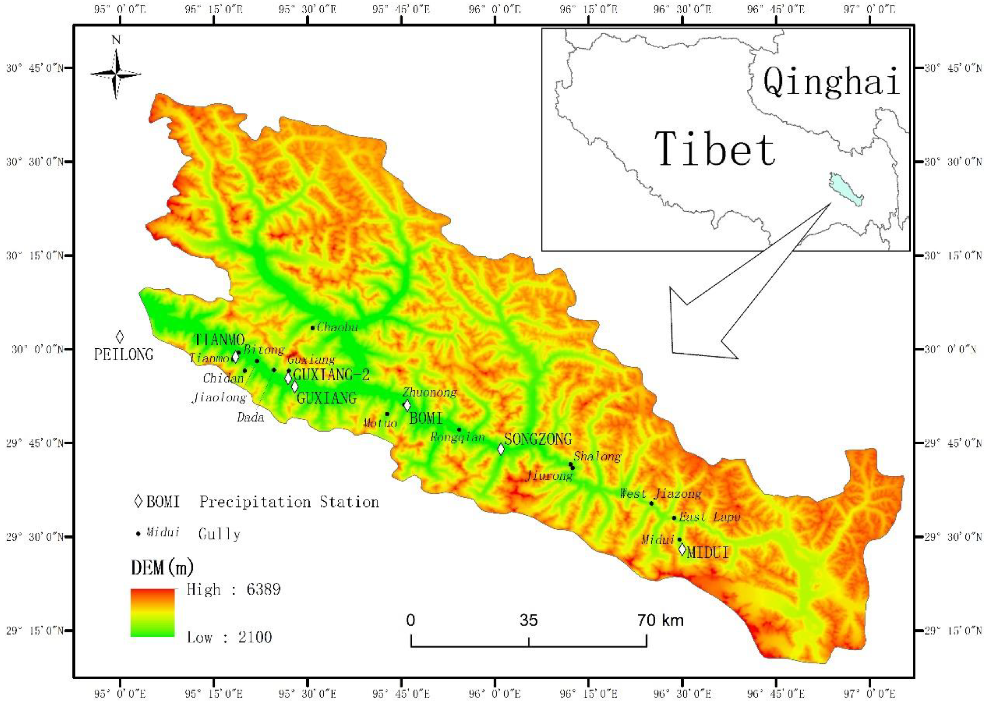
According to literature investigation, field investigation and observation, a certain number of debris flow records have accumulated in the Parlung Zangbo basin since the 1950s [29]. However, considering that global warming has caused significant changes in the local debris flow development environment [6], applicability of the early part of these data is limited. Thus, we selected 23 debris flow events that have occurred in 15 debris flow gullies in the Ranwu–Peilong section between 2012 and 2020 as the research objects (Figure 1,

Table 1. Debris flow events recorded in the study area from 2012 to 2020.

Gully No.	Gully	Area (km2)	Event No.	Date	Time	Possible Causes	Monitoring Station
1	Bitong	24	DF1	2016-09-05	06:30	Snowmelt, Precipitation	PEILONG
			DF2	2018-07-11	03:00	Snowmelt, Precipitation	GUXIANG
2	Chaobu	16	DF3	2017-08-03	17:00	Ice and Snow melt	GUXIANG
3	Chidan	28	DF4	2016-09-05	11:00	Snowmelt, Precipitation	PEILONG
4	Dada	3	DF5	2020-07-10	16:10	Snowmelt, Precipitation	TIANMO
5	East Lapu	4	DF6 *	2013-07-05	21:00	Snowmelt, Precipitation	MIDUI/ SONGZONG
			DF7 *	2014-07-24	20:00	Snowmelt, Precipitation
			DF8	2018-05-22	17:00	Snowmelt, Precipitation
6	Guxiang	25	DF9	2020-07-09	21:00	Ice and Snow melt	GUXIANG-2
7	Jiaolong	22	DF10	2016-09-05	——	Snowmelt, Precipitation	PEILONG
8	Jiurong	7	DF11 *	2014-08.18	23:00	Snowmelt, Precipitation	SONGZONG
			DF12 *	2014-08-23	02:00	Snowmelt, Precipitation
			DF13 *	2015-08-04	22:30	Snowmelt, Precipitation
			DF14 *	2015-08-20	07:40	Snowmelt, Precipitation
9	Midui	1	DF15 *	2015-08-19	23:30	Snowmelt, Precipitation	MIDUI/ SONGZONG
10	Motuo	3	DF16 *	2015-08-19	22:30	Snowmelt, Precipitation	BOMI/ SONGZONG
11	Rongqian	5	DF17 *	2015-08-19	18:30	Snowmelt, Precipitation	BOMI/ SONGZONG
12	Shalong	15	DF18 *	2015-08-19	21:00	Snowmelt, Precipitation	SONGZONG
13	Tianmo	18	DF19	2018-07-11	03:00	Snowmelt, Precipitation	GUXIANG
14	West Jiazong	2	DF20 *	2012-09-22	09:00	Snowmelt, Precipitation	MIDUI
			DF21 *	2013-07-05	21:00	Snowmelt, Precipitation
			DF22 *	2013-07-31	18:00	Snowmelt, Precipitation
15	Zhuonong	5	DF23 *	2015-08-19	19:20	Snowmelt, Precipitation	BOMI/ SONGZONG

Note: Data from Deng et al. [7], Zeng et al. [30], Li et al. [31], and field observation; * refers to the events used for training and validation.

). The gullies are characterized by a total area of 1–28 km², with their outlets elevated at 2400–3800 m and having an over 30° average slope. The bedrock of these gullies is composed of granite gneiss, slate and quartzite, and the low-altitude part of the gullies is basically a forest covered area [7]. These established the general geographical features of the regional periglacial debris flow gullies.

2.2. Method

The quantitative analysis methods used in this paper mainly include Pearson correlation analysis, Borderline Synthetic Minority Over-Sampling Technique (Borderline SMOTE), Random Forest (RF), and Support Vector Machine (SVM). Because these methods have many separate applications reported [13,14,15,32], in this study, we provided only the necessary introductions to the main machine learning algorithms.

2.2.1. Borderline SMOTE

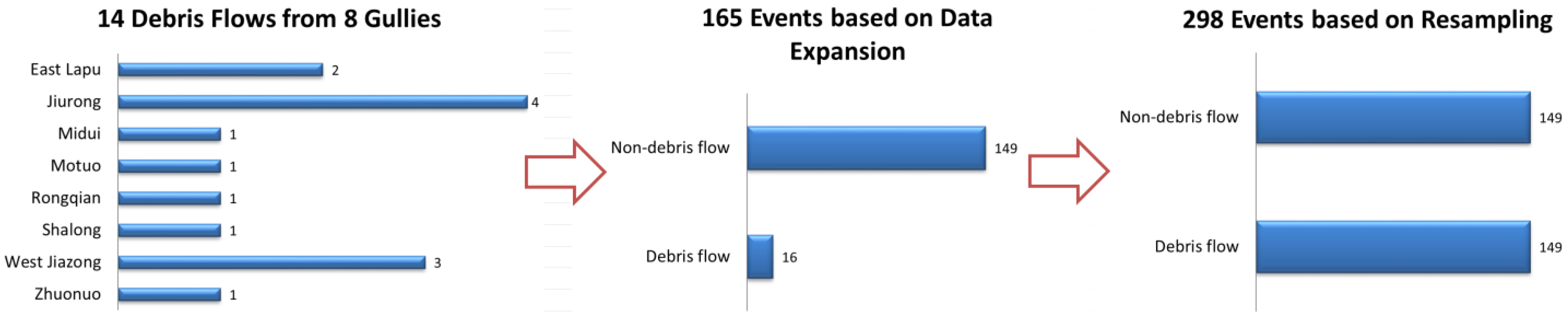
In this study, we summarized the prediction of debris flow occurrence into a bivariate classification problem, that is, the events with or without debris flow. Data from 23 debris flow events in 15 debris flow gullies were collected in the study area. Excluding the 9 events used for testing after 2015, only 14 events relevant to 8 gullies could be used for training and validation (Table 1). According to the monitoring results of the other gullies during a debris flow event period, we expanded the training data to 165 samples, of which 16 were positive samples of debris flow (12 events plus two events used twice by using two different but adjacent precipitation stations), and 149 were negative samples of non-debris flow (Figure 2). The ratio of positive and negative samples was close to 1:10. Hence, it was a typical imbalanced small sample data set. If these data were trained directly without special processing, it could be found that even if all positive samples were judged to be negative, the accuracy of the model, i.e., the ratio of correctly judged samples to the whole sample set here, still reached 91%, which was not the desired result. Therefore, we introduced a resampling technique for such data sets.

Commonly used resampling techniques include over-sampling and under-sampling. They can achieve the purpose of balancing data by directly copying minority class samples or subtracting redundant information from some of the majority class samples. Obviously, the over-sampling makes the decision boundary more specific and easily leads to overfitting, whereas the under-sampling directly reduces the potentially useful information. To eliminate these adverse effects, Chawla [23] proposed the Synthetic Minority Over-Sampling Technique (SMOTE); the fundamental idea of this technique is to extract several of the nearest congener samples b around the selected minority class center sample a and then interpolate any points on the ab line as the new synthetic samples.

Technically, SMOTE can alleviate the overfitting phenomenon caused by ordinary oversampling to a certain extent, but treating all minority samples equally also causes problems, such as high variance (overgeneralization) or data overlap of the new data sets. In addition, the classification idea of SVM tells us that the samples located at the decision boundary often play a decisive role in correct classification [33], and the expansion of these samples is usually more valuable. Accordingly, Hui [34] proposed an improved version of SMOTE (i.e., Borderline SMOTE), which can determine the decision boundary based on the proximity relationship between each minority sample and the surrounding majority samples. Then, only the minority samples near the boundary (i.e., the danger zone) can be interpolated linearly, such that the new data set can be more prominent in the decision boundary.

The method can be divided into two types (i.e., Borderline SMOTE-1 and Borderline SMOTE-2). The difference between these two types is that the Borderline SMOTE-1 performs ordinary SMOTE interpolation on the minority samples of danger zone after the decision boundary has been determined, whereas the Borderline SMOTE-2’s minority center samples will be connected with the neighboring majority samples for interpolating new samples. Theoretically, Borderline SMOTE-1 is more helpful to highlight the decision boundary. In this study, we used Borderline SMOTE-1 to interpolate the 16 positive samples from the 165 samples of the training set, to make the ratio of positive and negative samples 1:1. Then, a training set of 298 samples was obtained (Figure 2). The specific algorithm was implemented in Python.

2.2.2. Random Forest (RF)

The RF, a representative method of ensemble learning [35], was selected as one of the basic classifiers to avoid possible overfitting phenomenon. In essence, it is a collection of weak classifiers containing multiple decision tree structures. For classification, the algorithm generates a result through the “voting” of each decision tree [36]. RF can be regarded as an application extension of the information entropy theory. The construction of a decision tree (i.e., the basic unit of RF) follows the basic principle of rapidly reducing system entropy [37].

For a sample set, the Decision Tree model can take the following steps: First, the total value of information entropy of each feature will be calculated according to the probability that the attributes (such as high, medium, or low) of different input features (such as temperature, precipitation intensity, or slope) appear in each output category (e.g., the event occurs/does not occur). Second, based on the principle of rapidly reducing information entropy, the input feature with the most reduced information entropy is selected as the root node to classify the samples according to attribute differences of different features. If the output category corresponding to these samples is pure or single (e.g., debris flows occur in all samples with precipitation intensity exceeding 15 mm/h), the sample set under this attribute will not be subdivided downward as a leaf node. On the contrary, for the samples in non-leaf nodes, repeat these two steps until all the leaf nodes are generated.

Because the samples are inevitably mixed with noise data, the overfitting phenomenon may occur after the samples are completely subdivided into the final leaf nodes, which affects the generalization performance of the model [38]. Therefore, in the modeling process, the splitting scale of a decision tree generally can be controlled within a certain range based on specific principles or standards, such as setting a GainRatio rate or Gini coefficient. The RF resamples the number and feature of samples before building the decision tree, which means that each time, only part of the data in the total set is taken to build the tree [35]. In this way, many decision trees can be obtained according to the different samples collected. Because only part of the data in the total set is extracted each time, the interference of noisy data can be effectively reduced. Therefore, the probability of overfitting in the RF model is theoretically lower [35,39].

We used the RF plug-in in WEKA software to train, validate, and test the debris flow prediction model. Generally, it is believed that the two most important hyperparameters of RF modeling are the number of decision trees and the maximum number of features selected per sampling [40,41], i.e., numiterations and numfeatures in WEKA, respectively. The Gridsearch method was used to adjust the hyperparameters, firstly. However, it was found that for some algorithms, there was still the possibility of overfitting, or the given results consumed unnecessary computing power. In view of these situations, the hyperparameters were adjusted manually based on the results of Gridsearch so as to reduce calculation consumption while ensuring the accuracy. Finally, we determined that the numiterations was 70 and the numfeatures was 3. In addition, considering that the GainRatio can be used to reflect the relative importance of each feature, the GainRatio method was used to investigate the contribution of each indicator to the occurrence of debris flow in the preliminary indicator selection phase.

2.2.3. Support Vector Machine (SVM)

SVM is originally formulated as a binary classifier that obtains the optimal hyperplane by setting the maximum interval between the two classes of samples [33]. When using some specific modes, such as decomposing the multiclass datasets into multiple binary subsets, SVM can also be used to deal with multiclass problems. Because the setting of maximum interval requires only a small number of samples (i.e., the support vectors) that are closest to the hyperplane, this method is relatively friendly to small sample data sets [21]. The maximum interval can be classified into two types, i.e., the soft interval and the hard interval. The hyperplanes of the hard margin strictly distinguish all samples, which is suitable for linearly separable data sets. The soft margin means that a slack variable is added to select the optimal hyperplane on the premise of pursuing the maximum interval width. It is suitable for a data set that has a few outliers but is still linearly separable in general. When the data set is linearly non-separable, SVM introduces the kernel functions to map the samples into high-dimensional space, transform it into a linearly separable data set, and then finish the classification work.

The objective function of SVM not only has a loss function that reflects the accuracy of the fitting but also includes a regularization term that expresses the complexity of the model [25,33]. As a result, the optimization goal is not only to reduce the empirical risk but also to consider the structural risk of the model to avoid generating complex models that produce the overfitting phenomena due to the pursuit of local optima [42]. Thus, the generalization ability of the SVM model can be improved. The hyperparameters that need to be paid attention to in the actual operation of SVM are the C (penalty-factor) in the loss function term and the σ² in the kernel function (usually a Gaussian kernel function). The higher the C value is set, the greater the weight of the loss function term in the objective function, which will seek to further reduce the empirical risk, and then the model will be more prone to overfitting. Otherwise, the weight of the regularization term in the objective function is increased in a disguised way, and the generalization ability of the model will be strengthened, but there may be underfitting for the model classification. The higher the σ² value in the kernel function, the smoother the generated function, the more samples can become the support vectors, and the more likely the final model is to be underfitted.

This study used the LibSVM plug-in in WEKA to train, validate, and test the debris flow prediction model. According to the results of Gridsearch and manual tests, we decided to use the SVM model with radial basis kernel function for prediction, where gamma (corresponding to 1/2σ²) = 0.0001, and cost (corresponding to C) = 1. Using the weights generated by SVM for each feature in the process of solving the maximum interval, the relative importance of each feature could be calculated, i.e., the so-called SVM–RFE algorithm. This algorithm was employed to investigate the contribution of each indicator to the occurrence of debris flow. The linear SVM classifier (LibLINEAR plug-in in WEKA) was also introduced into the modeling to compare the performance of linear and nonlinear classifiers intuitively.

2.3. Data and Indicators

2.3.1. Data Sources

In this study, remote sensing and meteorological data with high availability were collected as the main information sources, mainly involving precipitation, temperature, landform, geology, vegetation, and snow cover (

Table 2. Data types and sources.

Type	Content	Sources
Precipitation	Hourly data of the stations of PEIlONG, BOMI, GUXIANG, SONGZONG, MIDUI on the day and the adjacent days of debris flow events in 2012–2018, and daily data of the 10 days before the event day; hourly data of GUXIANG-2 and TIANMO stations on the day and the adjacent days of debris flow events in 2020, and daily data of the 7 days before the event day	Data from 2012 to 2018 collected from the Bomi Geologic Hazard Observation Station of the Institute of Mountain Hazards and Environment, CAS; data of 2020 sourced from the field observation
Temperature	Daily maximum, minimum, and average data of Bomi station in 2012–2020 and Tianmo station in 2020 on the event day and the 15 days before the event day	Data of the Bomi station collected from the China Meteorological Data Service Centre; data of the Tianmo station sourced from the field observation
Landform	DEM of the Parlong Zangbo Basin	SRTM 90 m DEM and ASTER 30 m GDEMv2
Geology	National 1:2.5 million geological map of China	National Geological Archives Data Center, China
Vegetation Cover	NDVI of the study area in typical months from 2012 to 2020	MODIS 500 m monthly synthetic product
Snow Cover	Snow cover products from 2012 to 2015	Maximum_Snow_Extent MOD_Grid_Snow_500 m products of MOD10A2

).

2.3.2. Basic Indicators

-

Meteorology

In view of the natural relationships between the development of periglacial debris flow and the changes in precipitation and temperature, many scholars have explored the indicative factors of debris flow events according to these two factors. The precipitation indicators included antecedent precipitation, precipitation intensity, and precipitation duration, and the temperature indicators included accumulated temperature and average temperature. Based on outcomes from previous studies and the convenience of data collection [29,43,44,45], we selected 14 potential indicators, including accumulated effective precipitation over 3/5/10 days before the event (A₃/A₅/A₁₀), maximum and average precipitation intensity of the event day (before the event, of course, I_a/I_m), precipitation duration (D), temperature rise rate before the flood season (March to July normally, T_r), coefficient of variation of the daily temperature range over 5/10/15 days before the event (C_v⁵/C_v¹⁰/C_v¹⁵), antecedent three-day effective accumulated temperature (greater than 0 °C, T_a), and the average daily temperature over 5/10/15 days before the event (T₅/T₁₀/T₁₅).

The antecedent accumulated effective precipitation (A₃/A₅/A₁₀) was calculated based on the Antecedent Precipitation Index (API, formula 1, Deng et al. [7]).

r₀ = kr₁ + k²r₂ + k³r₃ + …+kⁿr_n

(1)

where r₀ is the antecedent accumulated effective precipitation (mm) of the event day (day 0); k is a constant reflecting surface runoff, which is related to soil texture and infiltration capacity; and rn is the maximum regional precipitation (mm) on the nth day before day 0.

It has been reported that the moraine soil in the study area was coarse in general [46], which was consistent with results from the field investigation of this research (Figure 3). Accordingly, it was considered that the gully soil of the study area had good permeability, and the two parameters (i.e., n and k) of the formula were set as 3 and 0.5 (A₃), respectively. In addition, the scenarios of n = 5/k = 0.6 (A₅) and n = 10/k = 0.7 (A₁₀) were set to understand the influence of different parameter settings on the prediction of debris flow events (

Table 3. Precipitation indicators data of related stations in training/validation phase (2012–2015).

No.	Precipitation Station	Year	Date	Event No. *	D (h)	I a (mm/h)	I m (mm/h)	A 3 (mm)	A 5 (mm)	A 10 (mm)
1	BOMI	2012	09-21	1	2	0.8	1.0	10.0	14.2	21.3
2		2012	09-22	1	1	1.0	1.0	5.8	9.4	16.2
3		2012	09-22	2	3	2.0	5.0	5.8	9.4	16.2
4		2012	09-22	3	13	1.4	4.0	5.8	9.4	16.2
5		2013	07-05	1	2	0.8	1.0	0.1	0.3	2.8
6		2013	07-05	2	9	2.1	4.5	0.1	0.3	2.8
7		2014	07-23	1	4	1.9	4.5	2.9	3.7	6.9
8		2014	07-24	1	1	1.5	1.5	5.7	7.2	10.7
9		2014	07-24	2	4	1.0	2.0	5.7	7.2	10.7
10		2014	07-24	3	4	1.8	3.5	5.7	7.2	10.7
11		2014	07-25	1	3	0.8	1.5	6.5	8.8	12.6
12		2014	08-18	1	1	1.0	1.0	4.4	8.5	14.7
13		2014	08-22	1	3	0.8	1.0	4.5	5.8	10.4
14		2014	08-22	2	1	1.0	1.0	4.5	5.8	10.4
15		2014	08-22	3	3	0.7	1.0	4.5	5.8	10.4
16		2014	08-22	4	2	1.3	1.5	4.5	5.8	10.4
17		2014	08-22	5	2	1.8	2.0	4.5	5.8	10.4
18		2014	08-23	1	14	1.0	3.5	7.3	9.4	14.1
19	SONGZONG	2012	09-21	1	3	1.2	1.5	10.8	15.5	22.5
20		2012	09-21	2	4	1.9	2.5	10.8	15.5	22.5
21		2012	09-22	1	11	2.9	7.0	12.5	17.7	25.8
22		2012	09-23	1	10	1.6	2.5	28.4	36.7	49.0
23		2013	07-05	1	5	1.3	3.0	0.8	0.9	2.8
24		2013	07-05	2	1	1.5	1.5	0.8	0.9	2.8
25		2013	07-06	1	4	1.8	3.0	6.4	7.7	10.3
26		2014	07-23	1	1	1.5	1.5	0.4	0.6	2.4
27		2014	07-24	1	3	1.0	1.5	0.9	1.2	2.7
28		2014	07-24	2	2	3.0	2.5	0.9	1.2	2.7
29		2014	08-18	1	2	5.0	2.5	2.7	6.4	11.7
30		2014	08-22	1	4	0.6	2.5	3.9	5.3	9.4
31		2014	08-23	1	9	2.4	5.0	8.6	11.5	16.2
32		2015	08-03	1	2	4.0	2.5	0.0	0.0	0.2
33		2015	08-04	1	3	3.2	6.0	6.5	7.8	9.1
34		2015	08-04	2	2	3.8	5.0	6.5	7.8	9.1
35		2015	08-17	1	2	1.0	1.0	1.0	1.3	2.1
36		2015	08-17	2	3	1.2	1.5	1.0	1.3	2.1
37		2015	08-17	3	4	0.6	1.0	1.0	1.3	2.1
38		2015	08-18	1	1	1.0	1.0	7.0	8.6	10.3
39		2015	08-19	1	9	1.1	2.0	11.4	14.7	18.3
40		2015	08-19	2	10	2.5	6.0	11.4	14.7	18.3
41	MIDUI	2012	09-22	1	17	1.3	3.0	3.9	5.9	10.3
42		2012	09-22	2	13	1.2	3.0	3.9	5.9	10.3
43		2012	09-23	1	1	1.5	1.5	15.6	19.9	26.3
44		2012	09-23	2	9	1.5	5.5	15.6	19.9	26.3
45		2013	07-04	1	4	1.8	2.5	0.0	0.0	1.4
46		2013	07-05	1	2	1.5	1.5	2.8	3.3	4.8
47		2014	07-23	1	1	1.0	1.0	1.6	2.3	3.7
48		2014	07-23	2	2	1.0	1.0	1.6	2.3	3.7
49		2014	07-23	3	2	1.3	1.5	1.6	2.3	3.7
50		2014	07-24	1	6	2.1	3.5	3.4	4.7	6.4
51		2014	08-22	1	4	0.8	1.0	0.9	2.1	5.4
52		2014	08-23	1	9	1.7	2.5	3.1	4.5	7.3
53		2014	08-24	1	8	1.6	3.5	8.6	11.2	15.1

Note: * means event number on that day.

).

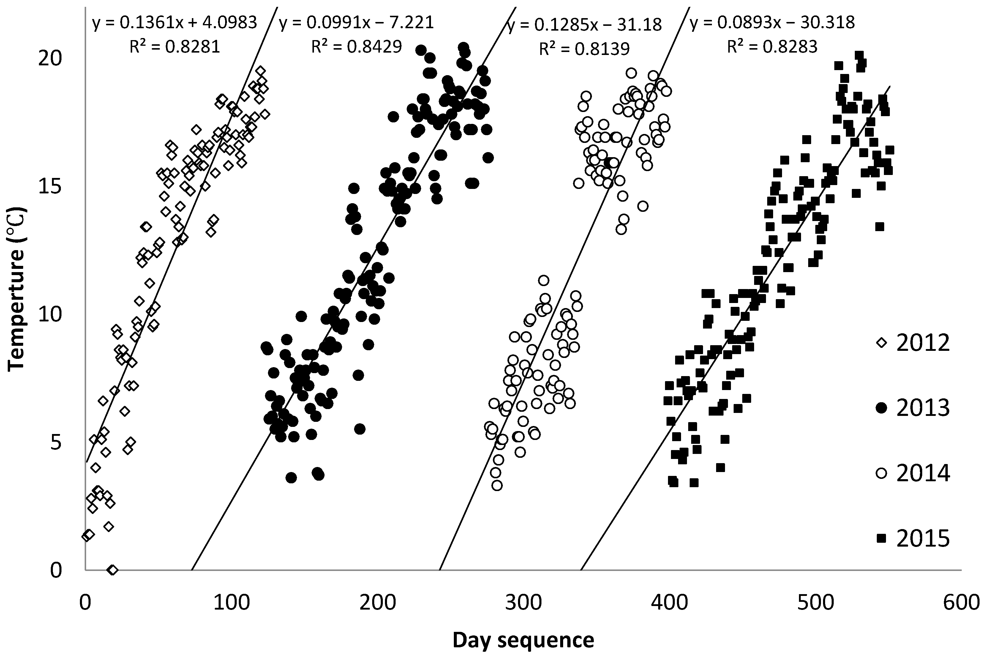
Considering that the debris flow events in the study area mainly occurred from July to September, the event may have been related to the amount of ice and snow melting from March or April every year. Therefore, we selected the daily average temperature and days from March to July of each year to construct the scatter diagram and used the slope of the linear trend equation of the scatter diagram to reflect the temperature rise rate in this period (Figure 4) and to obtain the indicator of the temperature rise rate before the flood season (T_r).

Assuming that the more severe the temperature change before the event, the more conducive it would be to freeze–thaw erosion and loose material accumulation, we added the coefficient of variation of the daily temperature range over 5/10/15 days before the event (C_v⁵/C_v¹⁰/C_v¹⁵), which were calculated by the coefficient of variation of the difference between daily maximum temperature and minimum temperature over 5/10/15 days (

Table 4. Temperature indicators data of BOMI station in training and validation phase in 2012–2015 (unit: °C).

Year	Date	C v 5	C v 10	C v 15	T 5	T 10	T 15	T a
2012	09-22	0.29	0.37	0.37	14.1	13.7	14.4	43.3
2012	09-21	0.30	0.38	0.38	13.8	13.8	14.6	44.0
2012	09-23	0.40	0.44	0.41	13.9	13.4	14.1	39.6
2013	07-06	0.11	0.26	0.29	18.7	17.5	17.5	56.8
2013	07-04	0.14	0.33	0.30	17.9	16.8	17.5	55.8
2013	07-05	0.11	0.29	0.30	18.5	17.2	17.6	56.4
2013	07-31	0.26	0.30	0.33	18.5	18.0	17.8	54.3
2014	07-23	0.23	0.34	0.29	18.1	17.2	17.6	56.6
2014	07-25	0.23	0.24	0.30	18.2	17.2	17.4	53.6
2014	07-24	0.20	0.36	0.30	18.4	17.1	17.5	55.1
2014	08-18	0.55	0.39	0.32	14.6	16.3	17.2	42.0
2014	08-22	0.26	0.42	0.35	16.3	15.6	16.5	48.9
2014	08-23	0.30	0.41	0.35	16.0	15.3	16.2	45.8
2014	08-24	0.35	0.42	0.36	15.6	15.0	16.0	44.2
2015	08-04	0.15	0.19	0.25	17.3	17.2	16.6	54.6
2015	08-03	0.14	0.19	0.25	17.0	16.8	16.5	53.4
2015	08-17	0.31	0.37	0.31	18.8	17.9	17.9	54.2
2015	08-18	0.46	0.41	0.38	18.0	18.0	17.7	50.6
2015	08-19	0.46	0.49	0.43	17.0	17.9	17.6	47.8
2015	08-20	0.38	0.53	0.48	15.9	17.5	17.3	44.4

). To further investigate the influence of short-term temperature change on the development of periglacial debris flow, the indicators of antecedent three-day effective accumulated temperature (greater than 0 °C, T_a) and the average of daily temperature over 5/10/15 days before the event (T₅/T₁₀/T₁₅) were also calculated.

-

Topography

Topographic relief has had a great influence on runoff generation and flow confluence as well as on the storage and release of gravitational potential energy from loose materials. Hence, it is one of the preconditions for the development of periglacial debris flow. In this study, we selected five indicators, including watershed height difference (H_d), gully gradient of mainstream (G_g), concave or convex characteristic from longitudinal profile (P), watershed average slope (S_a), and slope aspect (A_s), to reflect the influences of topographic factors (

Table 5. Topographic and geological characteristics of the eight debris flow gullies in the training set.

Gully	Hd (m)	Sa (°)	Gg (°)	As	P (%)	F	L
Zhuonong	1832.62	32	11.4	East–Northwest	−65.5	0.33	Extremely hard
West Jiazong	1858.96	37	34.0	South–Southwest	−12.6	0.00	Extremely hard
Shalong	1508.94	32	13.4	Southwest–West	−3.8	0.31	Secondary hard
Rongqian	1993.82	32	29.4	South–Southwest	−4.9	0.10	Extremely hard
Motuo	1510.14	27	28.6	East–Southeast	−2.2	0.25	Extremely hard
Midui	1262.14	34	31.8	East–Northeast	4.2	0.33	Secondary hard
Jiurong	1751.91	36	23.5	West–Northwest	−28.0	0.21	Secondary hard
East Lapu	1563.89	36	30.1	South–Southwest	3.1	0.10	Extremely hard

).

In practice, the longitudinal profile of the gully mainstream was extracted first using the three-dimensional analyst function in GIS. Then, we obtained H_d by calculating the difference between the outlet elevation and maximum elevation; calculated G_g from the ratio of Hd to the projection length of the longitudinal profile by arctangent function transformation; characterized P by a quantitative method (Formular 2); and obtained S_a by calculating the average slope using the zonal statistical function of GIS. The A_s was summarized based on several main slope aspects of each watershed.

P = (a₁ − a₂) / a₂

(2)

where P is the concave or convex characteristic of a longitudinal profile (%), and a positive value means that the profile is mainly convex, whereas a negative value is opposite; a₁ is the area of the profile; and a₂ is the triangle area enclosed by the three vertices of the profile.

-

Geology

Geological indicators included lithologic hardness (L) and fault buffer (F, Table 5). The indicator of L, mainly hard and sub-hard, was qualitatively classified based on field investigation and the 1:2.5 million national geological map. The study area had many faults according to the map, among which the most famous one named Jiali-Ranwu fault was distributed in the south of the area, and the rest were mostly unproved faults. According to the fault data provided by the map, we scored five buffers (1 km, 2 km, 3 km, 5 km, and 10 km) according to the distance to the fault (Figure 5), and then, the average value of each gully watershed was extracted and normalized using the zonal statistics function of GIS to obtain the F value.

-

Underlying surface

Snow melting is one of the basic reasons for the formation of periglacial debris flow [1,10]; thus, the change of snow cover is an important consideration in the underlying surface conditions. In contrast, the influence of vegetation on periglacial debris flow development is more complicated. On the one hand, vegetation can enhance the strength of soil by root system [47], and the hydrological effect of vegetation, such as intercepting rainfall and extracting soil moisture, is also conducive to the stability of a slope [48]. On the other hand, the surcharge load caused by plant weight and the transmission of drag force from wind reduce the slope stability [49,50]. Therefore, vegetation can promote or inhibit the formation of debris flows by increasing or reducing the supply of loose materials to a certain extent.

For the study area, vegetation can hardly affect the initiation of loose materials in the glacier area. However, the forests in the low-altitude valley may play an important role on the development of periglacial debris flow. Hence, the effects of vegetation and snow cover would be focused on this part, including four indicators: antecedent spatial scale Normalized Difference Vegetation Index (NDVI_s), antecedent temporal scale NDVI (NDVI_t), average maximum snow cover rate (MSC_a), and antecedent snow cover decrease rate (ASC_d). Among them, we calculated the antecedent NDVI indicators, basically, the vegetation coverage of each gully watershed in the month before the debris flow events in 2012–2020, based on the monthly synthetic product of MODIS 500 m NDVI (

Table 6. NDVI changes of 15 debris flow gullies in the study area from 2012 to 2020.

Gully	NDVI
	Training/Validation Phase				Testing Phase
	2012-08	2013-06	2014-07	2015-07	2016-08	2017-07	2018-04	2018-06	2020-07
Tianmo	0.12	0.18	0.20	0.70				0.40	0.51
Chidan	0.23	0.37	0.31	0.75	0.69
Jiaolong	0.12	0.16	0.17	0.51	0.37
Chaobu	0.13	0.20	0.52	0.83		0.64
Bitong	0.12	0.18	0.20	0.51	0.44			0.29	0.39
Dada	0.16	0.19	0.43	0.61					0.39
Guxiang	0.12	0.17	0.19	0.42		0.30		0.28
Zhuonong	0.24	0.48	0.31	0.69
West Jiazong	0.16	0.42	0.28	0.43
Shalong	0.18	0.27	0.23	0.38
Rongqian	0.24	0.34	0.22	0.51
Motuo	0.29	0.47	0.38	0.62
Midui	0.06	0.11	0.08	0.16
Jiurong	0.34	0.41	0.42	0.57			0.22
East Lapu	0.26	0.30	0.23	0.32			0.04

). Considering that both interannual and regional differences on vegetation coverage were significant, the NDVI_t and NDVI_s were obtained by normalizing the annual and regional sequences, respectively, to reflect the impact of this factor comprehensively.

Based on the products of MOD10A2 from 2012 to 2015, we calculated the proportion of snow and cloud cover area of each watershed at training and validation phase, respectively. The layers with more than 5% cloud were removed in this process, and the proportion of the largest snow coverage area before the debris flow events was selected as the maximum snow coverage rate of the current year. According to the difference between this maximum rate and the latest snow coverage rate before the event, the ASC_d could be calculated, and the MSC_a could also be obtained based on the average statistics of this maximum rate from 2012 to 2015 (

Table 7. Snow cover conditions of the eight debris flow gullies at training and validation phase in 2012–2015 (unit: %).

Gully	ASCd				MSCa
	2012	2013	2014	2015
Zhuonong	89.2	93.6	86.0	93.0	86.5
West Jiazong	84.3	91.6	100.0	80.0	98.5
Shalong	43.8	100.0	80.1	94.5	93.1
Rongqian	93.7	100.0	83.9	79.5	77.5
Motuo	90.9	100.0	86.3	100.0	100.0
Midui	80.0	90.0	80.0	100.0	100.0
Jiurong	100.0	100.0	82.3	100.0	92.4
East Lapu	91.4	91.4	100.0	96.0	90.9

).

Based on the above-mentioned 25 indicators and the watershed area (A) of each gully, a total of 26 preliminary indicators were selected and normalized for subsequent analysis.

3. Results and Discussion

3.1. Selection of Prediction Indicators

To avoid the possible interference from over-resampling, 165 events data without resampling were used here for further indicator selection. Based on the principle of reducing the indicators as much as possible and high operability, different methods such as Pearson correlation and SVM-RFE were employed to determine the final indicators to be included in the classification model.

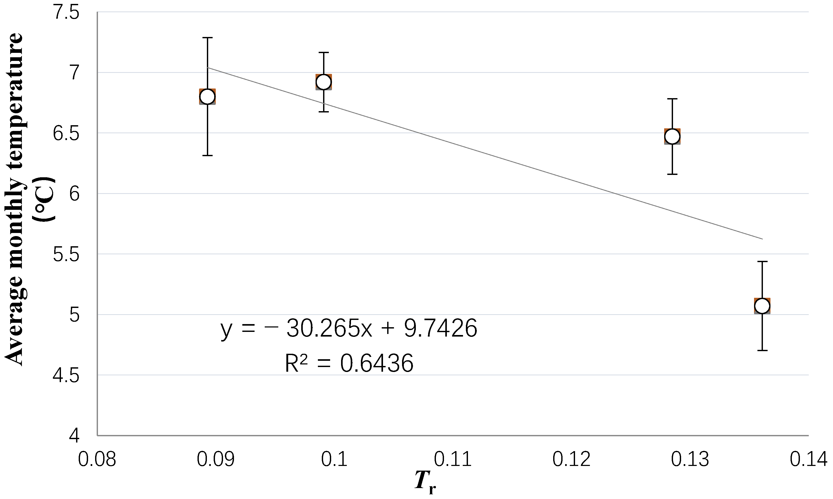
First, we used Pearson correlation analysis to eliminate the variables with obvious false correlation; that is, the correlation that cannot reflect the true relationship between the two variables, even if it is statistically significant. The results indicated that 13 indicators related to vegetation, temperature, and precipitation were significant with the development of periglacial debris flow in the study area (

Table 8. Assessment methods of indicator selection and related ranking.

Rank	Correlation Analysis		SVM-RFE		GainRatio
	Coefficient	Indicator	Average Merit	Indicator	Score	Indicator
1	0.42 **	NDVIt	23 ± 2.7	D	0.47	Cv10
2	−0.36 **	Tr	22.5 ± 3.0	T10	0.47	Cv15
3	0.34 **	D	21.4 ± 2.6	A5	0.26	Cv5
4	0.30 **	Cv15	21.2 ± 1.5	T15	0.24	A3
5	0.27 **	T10	20.3 ± 4.1	Cv15	0.24	Im
6	0.26 **	Im	20.3 ± 1.1	A10	0.16	NDVIt
7	0.25 **	A3	19.8 ± 1.9	Im	0.11	T10
8	0.24 **	Cv5	19.3 ± 2.1	Cv10	0.11	T15
9	0.24 **	Cv10	18.4 ± 1.4	NDVIt	0.11	D
10	0.23 **	A5	16.9 ± 5.2	Ia	0.06	Ia
11	0.22 **	Ia	15.1 ± 2.7	A3	0	A10
12	0.21 **	T15	14.1 ± 0.3	Sa	0	T5
13	0.19 *	A10	12.4 ± 1.0	Hd	0	A5
14	0.11	Sa	8.8 ± 3.2	ASCd	0	MSCa
15	0.08	T5	8.8 ± 4.3	Cv5	0	ASCd
16	0.06	ASCd	8.3 ± 2.8	T5	0	F
17	−0.06	L	8.1 ± 4.7	MSCa	0	P
18	0.039	A	6.8 ± 3.6	Gg	0	As
19	0.03	As	6.7 ± 1.9	As	0	NDVIs
20	−0.03	F	6.4 ± 2.65	P	0	Gg
21	−0.02	Ta	6.3 ± 3.55	NDVIs	0	A
22	−0.02	Hd	6.2 ± 3.25	Ta	0	Hd
23	0.02	P	5.7 ± 3.44	L	0	L
24	0.01	MSCa	4.1 ± 2.74	F	0	Sa
25	0.01	Gg	4.1 ± 3.05	A	0	Ta
26	0.01	NDVIs

Note: ** and * are the significance of 0.01 and 0.05, respectively.

left). Most of them presented a positive correlation except for the temperature rise rate before the flood season (T_r). As mentioned before, periglacial debris flows usually occur with the increase in temperature [6]. However, the relationship between T_r and debris flow events seemed to contradict this cognition: that is, the faster the warming, the fewer debris flow events. Further analysis showed that T_r was mainly related to the initial temperature in March of each year. The higher the initial temperature level, the more limited the space for subsequent warming, and the slower the warming rate (Figure 6), whereas a higher initial temperature may indeed lead to the increase in snow melting rate and the occurrence of periglacial debris flow. Therefore, for the indicator of T_r, its correlation with debris flow development cannot reflect the actual relationship between temperature rise rate and regional debris flow occurrence; thus, the indicator needed to be eliminated.

Furthermore, we employed SVM-RFE and the GainRatio method to investigate the importance of the remaining 25 indicators in debris flow development, in which the 10-fold cross-validation was used in SVM-RFE. The results showed that although the importance or correlation ranking of each indicator from the three methods was quite different, the top indicators were highly similar, mainly the temporal sequences related to vegetation, precipitation, and temperature. Conversely, the indicators reflecting the spatial heterogeneity of landform, geology, and watershed characteristics ranked lower in general, which might have been related to the range of selected sample data.

Statistically speaking, the method of sample expansion in this study limits the performance of indicators reflecting spatial heterogeneity to a certain extent. The data from 165 events collected here included 16 events with debris flow and 149 events without debris flow. The 16 events with debris flow were obtained based on eight gullies monitored by the stations of Bomi, Songzong, and Midui from 2012 to 2015 (Table 1), while the 149 events without debris flow were expanded from the same eight gullies on different dates. Taking the debris flow event on 23 August 2014 in Jiurong gully as an example, on the event day, if no debris flow was recorded in the other seven gullies, the seven gullies on 23 August 2014 would be registered as non-debris flow events. In addition, if no debris flow was recorded in the other seven gullies on the day of 22 August 2014 or 24 August 2014, the seven gullies on that day would also be registered as non-debris flow events. In this way, many gullies have experienced almost the same frequency of debris flow and non-debris flow events, and the difference of watershed indicators, such as the mainstream slope, among these eight debris flow gullies is much smaller than that between debris flow gullies and non-debris flow gullies [51,52]. Thus, it is difficult to find a significant correlation between the indicators reflecting spatial heterogeneity and debris flow events in such a data set.

According to the results from the three assessment methods (Table 8), indicators closely related to the development of periglacial debris flow were NDVI_t, D, I_m, I_a, C_v¹⁵, C_v¹⁰, C_v⁵, T₁₅, T₁₀, A₁₀, A₅, and A₃. Because the indicators in I_m/I_a, C_v¹⁵/C_v¹⁰/C_v⁵, T₁₅/T₁₀, and A₁₀/A₅/A₃ presented repeatability to some extent, we selected the indicator with the highest comprehensive ranking of each category as an input of the classification model. Considering that the comprehensive ranking of Sa was the highest among all spatial related indicators, the final seven indicators were D, I_m, C_v¹⁵, T₁₀, A₃, NDVI_t, and S_a.

3.2. Modeling and Comparative Analysis

3.2.1. Training and Validation

As mentioned in Section 2.2.1, after the indicator selection work, Borderline SMOTE-1 was used to obtained a balanced training set, and the data were imported into the RF, SVM and Linear SVM (LSVM) models as the inputs, respectively. We employed the 10-fold cross-validation to train and validate the binary classification process on whether the debris flow occurred. Simultaneously, the precision rate, recall rate, Matthews Correlation Coefficient (MCC), Receiver Operating Characteristic Curve (ROC) and other model assessment indices were employed to evaluate the performance of each classification model. The calculation formulas of the main assessment indices are as follows:

TPR or Recall = TP/(TP + FN)

(3)

FPR = FP/(FP + TN)

(4)

Precision = TP/(TP + FP)

(5)

F-Measure = 2·Precision·Recall/(Precision + Recall)

(6)

MCC = (TP·TN − FP·FN)/sqrt [(TP + FP)(TP + FN)(TN + FP)(TN + FN)

(7)

All these indices are based on a fundamental concept named confusion matrix (

Table 9. A typical confusion matrix.

True Class	Predicted Class
	+	−
+	TP	FN
–	FP	TN

Note: + and − are positive and negative cases, respectively.

), which is a form of contingency table showing the differences between the true and predicted classes for a set of labeled examples [53]. In the confusion matrix, TP and TN are the number of true positives and true negatives, respectively, indicating that the predicted values are the same as the true values, and the predicted values are positive and negative examples, respectively; FN and FP are the number of false negatives and false positives, respectively, indicating that the predicted values are opposite to the true values, and the predicted values are negative and positive, respectively.

The assessment indices can evaluate models from different aspects. The true positive rate (TPR) or recall rate reflects the ratio of correctly classified positive cases to the total number of positive cases [54]; the false positive rate (FPR) represents the ratio of misclassified negative cases to the total number of negative cases, i.e., the false alarm rate in early warning system. Precision refers to the ratio of true positive cases to all cases classified as positive. The F-Measure is the harmonic weighted average of precision rate and recall rate, reflecting the comprehensive situation of the two indices [54]. The MCC describes the correlation between the prediction set and the observation set, with a value range of −1 to 1, and it is regarded as one of the most adaptable comprehensive evaluation indices, which was applicable to imbalanced data sets [55]; and the AUC is the area under the ROC curve [53], reflecting the probability that a positive sample is correctly classified. A value of 1 meant that all positive samples can be correctly classified, and a value of 0.5 indicates that the performance of the classifier was no different from random classification. Except for the FPR, the higher the value of the assessment indices, the better the model classification performance.

The results showed that the RF-based model outperformed the SVM and LSVM-based model (

Table 10. Comparison of the results from different models on periglacial debris flow prediction.

Phase	Model	Class	TPR	FPR	Precision	F-Measure	MCC	AUC
Training and Validation	RF	No	0.966	0.013	0.986	0.976	0.953	0.997
		Yes	0.987	0.034	0.967	0.977
		WA	0.977	0.023	0.977	0.977
	SVM	No	0.886	0.034	0.964	0.923	0.855	0.926
		Yes	0.966	0.114	0.894	0.929
		WA	0.926	0.074	0.929	0.926
	LSVM	No	0.765	0.342	0.691	0.726	0.425	0.711
		Yes	0.658	0.235	0.737	0.695
		WA	0.711	0.289	0.714	0.711
Testing	RF	No	0.750	0.222	0.750	0.750	0.528	0.778
		Yes	0.778	0.250	0.778	0.778
		WA	0.765	0.237	0.765	0.765
	SVM	No	0.500	0.222	0.667	0.571	0.290	0.639
		Yes	0.778	0.500	0.636	0.700
		WA	0.647	0.369	0.651	0.639
	LSVM	No	0.375	0.111	0.750	0.500	0.311	0.632
		Yes	0.889	0.625	0.615	0.727
		WA	0.647	0.383	0.679	0.620

Note: “Yes” for debris flow events and “No” for non-debris flow events; WA represents weighted average.

). The values of recall rate, F-Measure, MCC, AUC, and other major assessment indices of the RF model in the training and validation phase all exceeded 0.95, and the prediction performance on positive and negative events was equivalent. Although the values of main assessment indices of the SVM model were also above 0.92, the recall rate of the negative events was 8% lower than that of positive events, the weighted FPR of the SVM model was more than three times higher than that of the RF model, and the MCC was also 10.3% lower than that of the RF model. As a typical linear classifier, LSVM lagged behind the SVM and RF-based model in almost all the assessment indices, reflecting the complexity of periglacial debris flow prediction.

Further analysis of the confusion matrix showed that the SVM model had 17 false predictions of negative events, which was much higher than that of the RF model, and the number of false predictions of positive events was also higher than that of the RF model (

Table 11. Comparison of results from different models on the confusion matrix.

Phase	Model	RF		SVM		LSVM
	Class	No	Yes	No	Yes	No	Yes
Training and Validation	No	144	5	132	17	114	35
	Yes	2	147	5	144	51	98
Testing	No	6	2	4	4	3	5
	Yes	2	7	2	7	1	8

). In short, although the overall prediction accuracy of the two models in the training and validation phase could reach a high level, the RF model was the preferred solution.

3.2.2. Testing

According to the RF, SVM and LSVM models established by the training and validation results, 17 events in 2016–2020 were imported into the model for testing (

Table 12. Prediction results of different models on the 17 events of the testing set.

No.	Gully	Date	Station	A 3	D	I m	NDVI t	S a	C v 15	T 10	Debris Flow	RF	SVM
1	Chidan	2016-09-05	PEILONG	21.75	15.00	4.70	0.69	30.70	0.43	16.80	Yes	√	√
2	Jiaolong	2016-09-05	PEILONG	21.75	15.00	4.70	0.37	36.20	0.43	16.80	Yes	√	√
3	Bitong	2016-09-05	PEILONG	21.75	15.00	4.70	0.44	34.50	0.43	16.80	Yes	√	√
4	Chaobu	2017-08-03	GUXIANG	3.10	1.00	0.20	0.64	35.00	0.17	18.30	Yes	√	×
5	Chaobu	2017-08-02	GUXIANG	0.09	6.00	1.60	0.64	35.00	0.17	18.40	No	√	√
6	Guxiang	2017-08-03	GUXIANG	3.10	1.00	0.20	0.30	35.60	0.17	18.30	No	√	√
7	East Lapu	2018-05-22	SONGZONG	0.00	0.00	0.00	0.04	36.00	0.21	14.00	Yes	×	×
8	East Lapu	2018-05-21	SONGZONG	0.00	0.00	0.00	0.01	36.00	0.21	13.10	No	√	√
9	Jiurong	2018-05-22	SONGZONG	0.00	0.00	0.00	0.22	36.00	0.21	14.00	No	√	√
10	Tianmo	2018-07-11	GUXIANG	12.94	10.00	3.10	0.40	37.70	0.24	18.20	Yes	√	√
11	Bitong	2018-07-11	GUXIANG	12.94	10.00	3.10	0.29	34.50	0.24	18.20	Yes	√	√
12	Guxiang	2018-07-11	GUXIANG	12.94	10.00	3.10	0.28	35.60	0.24	18.20	No	×	×
13	Dada	2020-07-09	TIANMO	0.65	2.35	6.00	0.39	33.00	0.37	16.26	No	√	×
14	Dada	2020-07-10	TIANMO	6.50	3.00	7.60	0.39	33.00	0.35	16.19	Yes	√	√
15	Tianmo	2020-07-10	TIANMO	6.50	3.00	7.60	0.51	37.70	0.35	16.19	No	×	×
16	Guxiang	2020-07-08	GUXIANG-2	0.20	0.00	0.00	0.39	35.60	0.37	15.98	No	√	×
17	Guxiang	2020-07-09	GUXIANG-2	0.35	3.80	2.33	0.39	35.60	0.37	16.26	Yes	×	√

). The results showed that the MCC and AUC of the RF model were 82% and 22% higher than those of the SVM model, respectively (Table 10). Combined with the confusion matrix of the test set (Table 11), it can be found that the prediction performance of both models on debris flow events is good, and the recall rate can reach more than 0.77. The disadvantage of SVM is reflected in the prediction of non-debris flow events: the recall rate is only 0.5, which is much lower than that of RF (0.75).

Compared with the performance in the training and validation phase, the LSVM-based model performed significantly better in this phase, and some assessment indices were even higher than that from the RF or SVM model. However, this is mainly because the model predicted 13 of the 17 events as debris flow, which improved the recall rate of debris flow events (0.889) but also enlarged the false alarm rate (0.625) simultaneously (Table 10). The LSVM has no kernel function processing procedure, so it is only applicable to the linearly separable datasets [21,33]. For the complex data set in this case, the classifier is not competent for this prediction task.

If we focus on the prediction results of each event (Table 12), it can be found that the outputs of the RF and SVM models are more sensitive to the precipitation indicators, especially A₃ (0.79 ** for RF and 0.573 * for SVM on Pearson correlation coefficient, the same below) and I_m (0.587 * for RF and 0.726 ** for SVM). In addition, the response of SVM to temperature indicator is also outstanding, especially for C_v¹⁵ (0.787 **). Taking the outputs as the dependent variable and the seven indicators as the independent variable for stepwise regression, the results showed that the goodness of fit from the SVM model was higher than that from the RF model (

Table 13. Main model parameters of the stepwise regression analysis based on test set.

Dependent Variable	Independent Variable	Standardized Coefficients	t-Value	p-Value	F-Value	Adjusted R2
RF outputs	A3	0.790	4.986	0.000	24.862	0.599
SVM outputs	Cv15	0.818	5.891	0.000	19.167	0.694
	T10	0.338	2.433	0.029

). Although the processing mechanism of nonparametric models (such as SVM and RF) does not depend on the correlation between the input and output, the prediction result of SVM in this case seems to be closer to the linear relationships between the indicators and the events, even with the support of kernel functions.

The key of success classification for SVM is to find the support vectors. Borderline SMOTE highlights the decision boundary through interpolation, so it is more conducive to the classification of the SVM model, theoretically [19,56]. Actually, the optimal hyperparameter value of gamma given by Gridsearch was 0.001. Under this condition, the weighted recall rate, MCC, and AUC of SVM were 0.977, 0.953, and 0.977, respectively, which was basically as good as those of the RF model. However, the model classified 16 of the 17 test events into non-debris flow events, resulting in the recall rate of debris flow events being only 0.11, i.e., the overfitting occurred. This indicates that the SVM algorithm is still prone to overfitting even if the Borderline SMOTE is applied, whereas the RF shows better robustness at this point, partly because it is relatively less sensitive to the hyperparameter setting [57].

Some scholars believed that the ensemble learning-based RF model was insensitive to the lack of input data [58]. In other words, even if there was no process of indicator selection, theoretically, the model established by all indicators had a higher probability of making an effective prediction, even in the absence of some input indicators in the testing phase. In this study, we also tested the RF model built by 26 full indicators. The results showed that the performance of the full indicator model was basically the same as that of the simplified model in the phases of training, validation, and testing, presenting no advantage in prediction accuracy. Moreover, full indicator modeling would have increased the amount of calculation and affected the speed of model construction and response. Considering the performance of the model and the cost of data collection and processing, the early warning efficiency of the simplified model was obviously higher.

Another thing worth noting is that although the RF model shows acceptable accuracy in this phase, there are still some shortcomings. First, the prediction effect for debris flow events without precipitation is still poor, such as the seventh event in Table 12. Second, the model takes the indicators reflecting spatial heterogeneity into account, but the influences of these indicators are limited in prediction. For example, the Dada gully and adjacent Tianmo gully share the same precipitation station; thus, most monitoring data are identical except the NDVI_t and S_a. However, for the events on 10 July 2020, the model cannot distinguish whether debris flow occurred in these two gullies only based on the data difference of this degree (Table 12). Therefore, the model proposed in this paper is still a regional prediction model, and its spatial resolution cannot be accurate to specific gullies at present.

3.2.3. Comparison

I-D Model and I-D-A Model

The rainfall indicator method is currently the most widely used debris flow monitoring and early warning method in the world. Its representative method is the power law equation (I-D method) proposed by Caine [59]. This method assumes that the critical rainfall intensity for debris flow is nonlinear with the rainfall duration. As the rainfall duration increases, the critical rainfall intensity decreases accordingly. The traditional I-D method does not consider the impact of antecedent rainfall, so its prediction accuracy may be poor for watersheds with better vegetation coverage and greater water storage potential. Fortunately, the so-called I-A method based on the relationships between antecedent effective rainfall and rain intensity can make up for this shortcoming [7]. However, some scholars have pointed out that the warning effect of the I-D method is better than that of the I-A method for sandy soil areas with strong infiltration capacity [60].

The proposed RF model, i.e., the original model here, is essentially an event-based prediction model for periglacial debris flow. By introducing the antecedent effective cumulative precipitation (A₃) of each event, the model can simultaneously consider the effects of antecedent precipitation (A₃), precipitation duration (D), and precipitation intensity (I_m) on the development of debris flow. Therefore, it is actually an I-D-A model. Herein, we tested and compared the performance of the original model and the RF model without A₃, i.e., the I-D model in this paper. The results showed that the advantage of the I-D-A model in the training and validation phase was not obvious, and the difference between them was less than 3% in MCC, which was the assessment index with the largest difference. On the contrary, in the testing phase, the classification accuracy of the I-D-A model was significantly higher than that of the I-D model, and the difference between them in MCC was more than two-fold. Without the support of A₃, the false alarm rate for both positive and negative samples increased (

Table 14. Comparison of prediction performance of RF models in different conditions.

Phase	Model	Class	TPR	FPR	MCC	ROC
Training and Validation	Original	No	0.966	0.013	0.953	0.997
		Yes	0.987	0.034
		WA	0.977	0.023
	Without A3	No	0.946	0.020	0.927	0.995
		Yes	0.980	0.054
		WA	0.963	0.037
	Non-resample	No	0.980	0.375	0.664	0.947
		Yes	0.625	0.020
		WA	0.945	0.341
	SMOTE	No	0.966	0.028	0.939	0.995
		Yes	0.972	0.034
		WA	0.969	0.031
Testing	Original	No	0.750	0.222	0.528	0.778
		Yes	0.778	0.250
		WA	0.765	0.237
	Without A3	No	0.500	0.333	0.169	0.736
		Yes	0.667	0.500
		WA	0.588	0.422
	Non-resample	No	0.750	0.667	0.091	0.729
		Yes	0.333	0.250
		WA	0.529	0.446
	SMOTE	No	0.750	0.556	0.203	0.750
		Yes	0.444	0.250
		WA	0.588	0.394

Note: “Yes” for debris flow events and “No” for non-debris flow events; WA represents weighted average.

). Considering that this result is obtained even in the area with good infiltration condition, which is reported as more suitable for the I-D model [60], it is believed that the antecedent precipitation index is of great significance to improve the performance of debris flow prediction model, at least in this case.

Resampling Model and Non-Resampling Model

Previous studies have found that because of the modeling idea and model structure, some machine learning algorithms are inherently capable of dealing with the imbalanced data sets to some extent [19,59]. For this type of algorithm, such as the RF, even if the original data are not resampled, a satisfactory classification result may be obtained. Herein, we tested the RF model with the original non-resampled data. The results showed that the resampling processing in this case was essential to improve the performance of the model. In the training and validation phase, although the recall rate of the debris flow event was only 0.625, the weighted recall rate exceeded 0.94 because of the larger weights on the non-debris flow event. This resulted in the model predictions being more biased toward non-debris flow events during the testing phase (

Table 15. Confusion matrix of prediction results of RF models in different conditions.

Model	Phase	Training & Validation		Testing
	Class	No	Yes	No	Yes
Original	No	144	5	6	2
	Yes	2	147	2	7
Without A3	No	141	8	4	4
	Yes	3	146	3	6
Non-resample	No	146	3	6	2
	Yes	6	10	6	3
SMOTE	No	144	5	6	2
	Yes	4	140	5	4

). Compared with the original model that had been resampled, the MCC of the non-resampled model had dropped by 32% in the training and validation phase, and the drop in the testing phase had reached 83%. The negative effect brought by the imbalanced data set was very significant.

SMOTE Model and Borderline SMOTE Model

The SMOTE is an intelligent oversampling algorithm commonly used in the current academic community, and the Borderline SMOTE, as an improved version of SMOTE, theoretically has a higher interpolation efficiency at the classification boundary. Using the SMOTE from WEKA to expand the original 16 debris flow events by eight times, the ratio of debris flow events to non-debris flow events was close to 1:1. We tested the RF model built by this data set and compared it with the original model using Borderline SMOTE. The results showed that in the training and validation phase, the SMOTE-based model had almost the same performance as the original model (Table 14). In the testing phase, however, the SMOTE-based model has a significantly lower recall rate for debris flow events (Table 15), and its MCC was only 38% of the original model. The use of Borderline SMOTE modeling is of practical significance for the improvement of prediction accuracy in this case.

Based on the results of the three tests, it can be found that the situation with/without the A₃ test and the SMOTE/Borderline SMOTE test is similar; that is, the original model presents obvious advantages only in the testing phase. This is partly due to the lack of data in the testing set. However, it should also be noted that in each test, the assessment indices of the original model were ahead of the other models in all phases (Table 14), indicating that these two measures did improve the model prediction performance. On the contrary, the result of whether to resample the test is quite different from that of the other two tests. Regardless of the training and validation phase or the testing phase, the performance of the model using the resampling technique (whether ordinary SMOTE or Borderline SMOTE) is much better than that of the model without resampling, which indicates that the technique is necessary for preprocessing the original small and imbalanced data set.

4. Conclusions

Taking 15 typical periglacial debris flow gullies in the Parlung Zangbo Basin of southeast Tibet as an example, this study preliminarily explored how to establish a periglacial debris flow prediction model with acceptable accuracy and certain promotion value under the constraints of insufficient mechanism knowledge and imbalanced small sample data. Through field investigation and geostatistical analysis, a comprehensive index system covering 26 indicators from vegetation, meteorology, geology, and geomorphology was constructed firstly, and then seven of the indicators were selected as the recommended monitoring and early warning indicators, which were used as the inputs of the classification model after resampling. In addition, several comparative tests were also carried out for understanding the performance of the established model, and the following conclusions were drawn.

For the periglacial debris flow gully in the Peilong–Ranwu section of the Parlung Zangbo Basin, various temperature and precipitation indicators, as well as vegetation coverage, were closely related to the development of debris flow. Seven indicators, i.e., (1) precipitation duration (D), (2) maximum precipitation intensity (I_m), (3) coefficient of variation of the daily temperature range (C_v¹⁵), (4) antecedent temperature (T₁₀), (5) antecedent accumulated precipitation (A₃), (6) antecedent NDVI (NDVI_t), and (7) average slope (S_a), were recommended as the monitoring and early warning indicators.

Based on these seven indicators, we constructed the periglacial debris flow prediction model using the Borderline SMOTE and RF classification algorithm. The main assessment indices, such as the weighted recall ratio, MCC, and AUC, exceeded 0.95 in the training and validation phase, and most of them exceeded 0.7 in the testing phase, showing acceptable accuracy under the limited sample data. Therefore, it is considered that the proposed workflow and model, as a prediction scheme of regional precipitation-related periglacial debris flow, have a certain promotion value for further research.

The performance of the SVM-based prediction scheme in this case is also acceptable. However, compared with the RF scheme, the SVM scheme has a lower recall rate on non-debris flow events, which means that this scheme may lead to a higher false alarm rate. In addition, the SVM-based classification model may still have overfitting phenomenon under the interpolation of Borderline SMOTE, while the RF based on ensemble learning idea shows better robustness; that is, the model presents more stable performance under the condition of imbalanced small sample data interpolation.

For imbalanced small sample data sets, resampling is necessary to improve the classification accuracy of the model. In this case, the prediction results from the RF model without resampling were more biased toward non-debris flow events, because the non-debris flow events accounted for the majority of the data set. Compared with the RF model with resampling, the prediction accuracy of the model without resampling had dropped significantly, which could reach 83%.

The test results indicated that considering the antecedent accumulated precipitation in a precipitation event helped to improve the model prediction accuracy, even for an area with strong permeable sandy soil. Similarly, as an improved version of SMOTE, the application of Borderline SMOTE was also of positive significance to the improvement of model performance.

References

- Decaulne, A.; Saemundsson, P.; Petursson, O. Debris flow triggered by rapid snowmelt: A case study in the glei.arhjalli area, northwestern Iceland. Geogr. Ann. Ser. A Phys. Geogr. 2005, 87, 487–500. [Google Scholar] [CrossRef]
- Legg, N.T.; Meigs, A.J.; Grant, G.E.; Kennard, P. Debris flow initiation in proglacial gullies on Mount Rainier, Washington. Geomorphology 2014, 226, 249–260. [Google Scholar] [CrossRef]
- Wei, R.; Zeng, Q.; Davies, T.; Yuan, G.; Wang, K.; Xue, X.; Yin, Q. Geohazard cascade and mechanism of large debris flows in Tianmo gully, SE Tibetan Plateau and implications to hazard monitoring. Eng. Geol. 2018, 233, 172–182. [Google Scholar] [CrossRef]
- Kumar, A.; Bhambri, R.; Tiwari, S.K.; Verma, A.; Gupta, A.K.; Kawishwar, P. Evolution of debris flow and moraine failure in the Gangotri Glacier region, Garhwal Himalaya: Hydro-geomorphological aspects. Geomorphology 2019, 333, 152–166. [Google Scholar] [CrossRef]
- Liu, X.; Chen, B. Climatic warming in the Tibetan Plateau during recent decades. Int. J. Climatol. 2015, 20, 1729–1742. [Google Scholar] [CrossRef]
- Yu, G.-A.; Yao, W.; Huang, H.Q.; Liu, Z. Debris flows originating in the mountain cryosphere under a changing climate: A review. Prog. Phys. Geogr. Earth Environ. 2020, 45, 339–374. [Google Scholar] [CrossRef]
- Deng, M.; Chen, N.; Ding, H. Rainfall characteristics and thresholds for periglacial debris flows in the Parlung Zangbo Basin, southeast Tibetan Plateau. J. Earth Syst. Sci. 2018, 127, 11. [Google Scholar] [CrossRef] [Green Version]
- Gao, B.; Zhang, J.J.; Wang, J.C.; Chen, L.; Yang, D.X. Formation mechanism and disaster characteristics of debris flow in the Tianmo gully in Tibet. Hydrogeol. Eng. Geol. 2019, 46, 144–153. [Google Scholar]
- Gruber, S.; Haeberli, W. Permafrost in steep bedrock slopes and its temperature-related destabilization following climate change. J. Geophys. Res. Atmos. 2007, 112, F2. [Google Scholar] [CrossRef] [Green Version]
- Krautblatter, M.; Funk, D.; Günzel, F.K. Why permafrost rocks become unstable: A rock-ice-mechanical model in time and space. Earth Surf. Process. Landforms 2013, 38, 876–887. [Google Scholar] [CrossRef] [Green Version]
- Harris, C.; Davies, M.C.R.; Etzelmüller, B. The assessment of potential geotechnical hazards associated with mountain permafrost in a warming global climate. Permafr. Periglac. Process. 2001, 12, 145–156. [Google Scholar] [CrossRef]
- Iverson, R.; Vallance, J. New views of granular mass flows. Geology 2001, 29, 115–118. [Google Scholar] [CrossRef]
- Liang, W.-J.; Zhuang, D.-F.; Jiang, D.; Pan, J.-J.; Ren, H.-Y. Assessment of debris flow hazards using a Bayesian Network. Geomorphology 2012, 171–172, 94–100. [Google Scholar] [CrossRef]
- Staley, D.M.; Negri, J.A.; Kean, J.W.; Laber, J.L.; Tillery, A.C.; Youberg, A.M. Prediction of spatially explicit rainfall intensity–duration thresholds for post-fire debris-flow generation in the western United States. Geomorphology 2017, 278, 149–162. [Google Scholar] [CrossRef]
- Addison, P.; Oommen, T.; Sha, Q. Assessment of post-wildfire debris flow occurrence using classifier tree. Geomat. Nat. Hazards Risk 2019, 10, 505–518. [Google Scholar] [CrossRef] [Green Version]
- Walter, F.; Amann, F.; Kos, A.; Kenner, R.; Phillips, M.; de Preux, A.; Huss, M.; Tognacca, C.; Clinton, J.; Diehl, T.; et al. Direct observations of a three million cubic meter rock-slope collapse with almost immediate initiation of ensuing debris flows. Geomorphology 2020, 351, 106933. [Google Scholar] [CrossRef]
- Michie, D.; Spiegelhalter, D.J.; Taylor, C.C. Machine Learning, Neural and Statistical Classification; Citeseer: Princeton, NJ, USA, 1994. [Google Scholar] [CrossRef]
- Costache, R. Flash-Flood Potential assessment in the upper and middle sector of Prahova river catchment (Romania). A comparative approach between four hybrid models. Sci. Total. Environ. 2018, 659, 1115–1134. [Google Scholar] [CrossRef]
- Zhou, C.; Yin, K.; Cao, Y.; Ahmed, B. Application of time series analysis and PSO–SVM model in predicting the Bazimen landslide in the Three Gorges Reservoir, China. Eng. Geol. 2016, 204, 108–120. [Google Scholar] [CrossRef]
- Cui, Y.; Cheng, D.; Chan, D. Investigation of Post-Fire Debris Flows in Montecito. ISPRS Int. J. Geo-Inf. 2018, 8, 5. [Google Scholar] [CrossRef] [Green Version]
- Liu, Z.; Wang, L.; Zhang, Y.; Chen, C.P. A SVM controller for the stable walking of biped robots based on small sample sizes. Appl. Soft Comput. 2016, 38, 738–753. [Google Scholar] [CrossRef]
- Squarcina, L.; Villa, F.M.; Nobile, M.; Grisan, E.; Brambilla, P. Deep learning for the prediction of treatment response in depression. J. Affect. Disord. 2020, 281, 618–622. [Google Scholar] [CrossRef] [PubMed]
- Chawla, N.V.; Bowyer, K.W.; Hall, L.O.; Kegelmeyer, W.P. SMOTE: Synthetic Minority Over-sampling Technique. J. Artif. Intell. Res. 2002, 16, 321–357. [Google Scholar] [CrossRef]
- Schlögl, M.; Stuetz, R.; Laaha, G.; Melcher, M. A comparison of statistical learning methods for deriving determining factors of accident occurrence from an imbalanced high resolution dataset. Accid. Anal. Prev. 2019, 127, 134–149. [Google Scholar] [CrossRef] [PubMed]
- Cheng, D.; Wang, J.; Wei, X.; Gong, Y. Training mixture of weighted SVM for object detection using EM algorithm. Neurocomputing 2015, 149, 473–482. [Google Scholar] [CrossRef]
- Cheng, Z.L.; Liang, S.; Liu, J.K.; Liu, D.X. Distribution and change of glacier lakes in the upper Palongzangbu River. Bull. Soil Water Conserv. 2012, 32, 8–12. [Google Scholar]
- Liu, J.; Yao, X.J.; Gao, Y.P.; Qi, M.M.; Duan, H.; Zhang, D. Glacial Lake variation and hazard assessment of glacial lakes outburst in the Parlung Zangbo River Basin. J. Lake Sci. 2019, 31, 244–255. [Google Scholar]
- Lv, R.R.; Tang, B.X.; Zhu, P.Y. Debris Flow and Environment in Tibet; Press of Chengdu Science and Technology: Chengdu, China, 1999. [Google Scholar]
- Jia, Y. The Impact Mechanism of Climate Warming on Mountain Hazards in the Southeast Tibet. Ph.D. Thesis, University of Chinese Academy of Sciences, Beijing, China, 2018; pp. 118–143. [Google Scholar]
- Zeng, X.Y.; Zhang, J.J.; Yang, D.X.; Wang, J.C.; Gao, B.; Li, Y. Characteristics and Geneses of Low Frequency Debris Flow along Parlongzangbo River Zone: Take Chaobulongba Gully as an Example. Sci. Technol. Eng. 2019, 19, 103–107. [Google Scholar]
- Li, Y.L.; Wang, J.C.; Chen, L.; Liu, J.; Yang, D.; Zhang, J. Characteristics and geneses of the group-occurring debris flows along Parlung Zangbo River zone in 2016. Res. Soil. Water Conserv. 2018, 25, 401–406. [Google Scholar]
- Dong, L.-J.; Li, X.-B.; Peng, K. Prediction of rockburst classification using Random Forest. Trans. Nonferrous Met. Soc. China 2013, 23, 472–477. [Google Scholar] [CrossRef]
- Burges, C.J.C. A Tutorial on Support Vector Machines for Pattern Recognition. Data Min. Knowl. Discov. 1998, 2, 121–167. [Google Scholar] [CrossRef]
- Hui, H.; Wang, W.Y.; Mao, B.H. Borderline-SMOTE: A new over-sampling method in imbalanced data sets learning. In International Conference on Intelligent Computing; Springer: Berlin/Heidelberg, Germany, 2005; Volume 3644, pp. 878–887. [Google Scholar] [CrossRef]
- Breiman, L. Random forests. Mach. Learn. 2001, 45, 5–32. [Google Scholar] [CrossRef] [Green Version]
- Svetnik, V.; Liaw, A.; Tong, C.; Culberson, J.C.; Sheridan, R.P.; Feuston, B.P. Random Forest: A Classification and Regression Tool for Compound Classification and QSAR Modeling. J. Chem. Inf. Comput. Sci. 2003, 43, 1947–1958. [Google Scholar] [CrossRef]
- Quinlan, J.R. Introduction of decision trees. Mach. Learn. 1986, 1, 81–106. [Google Scholar] [CrossRef]
- Mitchell, T.M. Machine Learning; McGraw-Hill: Boston, MA, USA, 1997. [Google Scholar]
- Dimitriadis, S.I.; Liparas, D.; Dni, A. How random is the random forest? Random forest algorithm on the service of structural imaging biomarkers for Alzheimer’s disease: From Alzheimer’s disease neuroimaging initiative (ADNI) database. Neural Regen. Res. 2018, 13, 962–970. [Google Scholar] [CrossRef]
- Ming, D.; Zhou, T.; Wang, M.; Tan, T. Land cover classification using random forest with genetic algorithm-based parameter optimization. J. Appl. Remote. Sens. 2016, 10, 035021. [Google Scholar] [CrossRef]
- Zhou, T.N.; Ming, D.P.; Zhao, R. Land cover classification based on algorithm of parameter optimization random forests. Sci. Surv. Mapp. 2017, 42, 88–94. [Google Scholar]
- Vapnik, V. The Nature of Statistical Learning Theory; Springer: Berlin/Heidelberg, Germany, 1999. [Google Scholar]
- Rebetez, M.; Lugon, R.; Baeriswyl, P.A. Climatic change and debris flows in high mountain regions: The case study of the Ritigraben Torrent (Swiss Alps). In Climatic Change at High Elevation Sites; Diaz, H.F., Beniston, M., Bradley, R.S., Eds.; Springer: Dordrecht, The Netherlands, 1997; pp. 139–157. [Google Scholar]
- Chleborad, A.F. Use of Air Temperature Data to Anticipate the Onset of Snowmelt-Season Landslides (USGS Open-File Report 98-0124); US Geological Survey: Reston, VA, USA, 1998. [Google Scholar]
- Deng, M.; Chen, N.; Liu, M. Meteorological factors driving glacial till variation and the associated periglacial debris flows in Tianmo Valley, south-eastern Tibetan Plateau. Nat. Hazards Earth Syst. Sci. 2017, 17, 345–356. [Google Scholar] [CrossRef] [Green Version]
- Chen, N.S.; Wang, Z.; Tian, S.F.; Zhu, Y.H. Study on debris flow process induced by moraine soil mass failure. Quat. Sci. 2019, 39, 1235–1245. [Google Scholar]
- Greenway, D. Vegetation and Slope Stability. In Slope Stability: Geotechnical Engineering and Geomorphology; Anderson, M.G., Richards, K.S., Eds.; John Wiley and Sons Ltd: Hoboken, NJ, USA, 1987. [Google Scholar]
- Wilkinson, P.L.; Anderson, M.G.; Lloyd, D.M. An integrated hydrological model for rain-induced landslide prediction. Earth Surf. Process. Landforms 2002, 27, 1285–1297. [Google Scholar] [CrossRef]
- Coppin, N.J.; Richards, I.G. Use of Vegetation in Civil Engineering; Construction Industry Research and Information Association (CIRIA): London, UK, 1990. [Google Scholar]
- Emadi-Tafti, M.; Ataie-Ashtiani, B.; Hosseini, S.M. Integrated impacts of vegetation and soil type on slope stability: A case study of Kheyrud Forest, Iran. Ecol. Model. 2021, 446, 109498. [Google Scholar] [CrossRef]
- Takahashi, T. Debris Flow Mechanics, Prediction and Countermeasures; Taylor and Francis Group: London, UK, 2007; p. 108. [Google Scholar]
- Du, J.; Fan, Z.-J.; Xu, W.-T.; Dong, L.-Y. Research Progress of Initial Mechanism on Debris Flow and Related Discrimination Methods: A Review. Front. Earth Sci. 2021, 9, 629567. [Google Scholar] [CrossRef]
- Bradley, P. The use of the area under the ROC curve in the evaluation of machine learning algorithms. Pattern Recogn. 1997, 30, 1145–1159. [Google Scholar] [CrossRef] [Green Version]
- Fawcett, T. An Introduction to ROC analysis. Pattern Recogn. Lett. 2006, 27, 861–874. [Google Scholar] [CrossRef]
- Boughorbel, S.; Jarray, F.; El-Anbari, M. Optimal classifier for imbalanced data using Matthews Correlation Coefficient metric. PLoS ONE 2017, 12, e0177678. [Google Scholar] [CrossRef]
- Lee, T.; Kim, M.; Kim, S.-P. Improvement of P300-Based Brain–Computer Interfaces for Home Appliances Control by Data Balancing Techniques. Sensors 2020, 20, 5576. [Google Scholar] [CrossRef]
- Lei, C.; Deng, J.; Cao, K.; Xiao, Y.; Ma, L.; Wang, W.; Ma, T.; Shu, C. A comparison of random forest and support vector machine approaches to predict coal spontaneous combustion in gob. Fuel 2019, 239, 297–311. [Google Scholar] [CrossRef]
- Tang, Z.; Mei, Z.; Liu, W.; Xia, Y. Identification of the key factors affecting Chinese carbon intensity and their historical trends using random forest algorithm. J. Geogr. Sci. 2020, 30, 743–756. [Google Scholar] [CrossRef]
- Caine, N. The Rainfall Intensity—Duration Control of Shallow Landslides and Debris Flows. Geogr. Ann. Ser. A Phys. Geogr. 1980, 62, 23–27. [Google Scholar] [CrossRef]
- Abancó, C.; Hürlimann, M.; Moya, J.; Berenguer, M. Critical rainfall conditions for the initiation of torrential flows. Results from the Rebaixader catchment (Central Pyrenees). J. Hydrol. 2016, 541, 218–229. [Google Scholar] [CrossRef]
Figure 1.
Debris flow gullies and precipitation stations in the Ranwu–Peilong section of the Parlung Zangbo Basin.
Figure 2.
The preparation process of the data set for training and validation.
Figure 3.
Grain size characteristics of samples from typical debris flow gullies in field investigation.
Figure 4.
Scatter plot between daily average temperature and day sequence from March to July of each year (missing data for April 2012 and May 2014).
Figure 5.
Distribution of faults and their buffers in the study area.
Figure 6.
Relationship between Tr and the average temperature of March from 2012 to 2015 (with the Standard Error of Mean on daily average temperature of each March).