
Research on the Uplift Pressure Prediction of Concrete Dams Based on the CNN-GRU Model

School of Safety Science and Emergency Management, Wuhan University of Technology, Wuhan 430070, China
*
Author to whom correspondence should be addressed.
Water 2023, 15(2), 319; https://doi.org/10.3390/w15020319
Submission received: 27 November 2022
/
Revised: 5 January 2023
/
Accepted: 9 January 2023
/
Published: 12 January 2023
(This article belongs to the Special Issue Safety Monitoring and Management of Reservoir and Dams)
Abstract
:Dam safety is considerably affected by seepage, and uplift pressure is a key indicator of dam seepage. Thus, making accurate predictions of uplift pressure trends can improve dam hazard forecasting. In this study, a convolutional neural network, (CNN)-gated recurrent neural network, (GRU)-based uplift pressure prediction model was developed, which included the CNN model’s feature extractability and the GRU model’s learnability for time series correlation data. Then, the model performance was verified using a dam as an example. The results showed that the mean absolute errors (MAEs) of the CNN-GRU model were 0.1554, 0.0398, 0.2306, and 0.1827, and the root mean square errors (RMSEs) were 0.1903, 0.0548, 0.2916, and 0.2127. The prediction performance was better than that of the particle swarm optimization–back propagation (PSO-BP), artificial bee colony optimization–support vector machines (ABC-SVM), GRU, long short-term memory network (LSTM), and CNN-LSTM models. The method improves the utilization rate of dam safety monitoring results and has engineering utility for safe dam operations.
1. Introduction
Dams are the most important infrastructure in water conservancy and hydropower projects and play an active role in flood control, irrigation, shipping, and power generation. However, while dams bring great benefits, they also have a series of safety problems, and a dam failure can have serious social and economic consequences downstream, causing massive personal and property losses [1,2]. To reduce the damage caused by dam failure, dam safety monitoring has been carried out in various countries. Uplift pressure is one of the key tasks for monitoring the seepage of concrete dams and plays an important role in reflecting the stability and durability of the dam [3,4]. Therefore, it is possible to improve the accuracy of the dam hazard occurrence forecast by combining historical uplift pressure-monitoring data with intelligent algorithms to establish a practical and effective concrete dam safety monitoring model.
The dam safety monitoring model is a mathematical model established to reflect the law of change in the amount of the effect of dam monitoring. Many studies have been conducted on dam safety monitoring models; however, most of them focus on displacement monitoring, whereas there are fewer theoretical research results devoted to uplift pressure-monitoring models. In addition, the current monitoring models used in practical engineering have problems, such as the poor adaptability of the monitoring model and prediction accuracy, that are insufficient for meeting intelligent target requirements. The traditional statistical model is employed as an example. Although the calculation is simple, it is difficult to reflect the nonlinear relationship between the effect size and complex factors. This results in poor extrapolation accuracy and low forecast accuracy [5]. In recent years, the study of dam safety monitoring models has been enriched by the development of artificial intelligence theory and the wide application of various intelligent algorithms in data analysis and mining [6].
Support vector machines (SVMs) give excellent performance in solving high-dimensional nonlinear problems [7], so they have been introduced into dam safety monitoring research by scholars. Rankovic V et al. used SVM for deformation prediction in the safety monitoring of concrete dams, and the application results of engineering examples show that SVM prediction accuracy is high [8]. SVMs are affected by parameters, so intelligent optimization algorithms, such as particle swarm optimization (PSO) and artificial bee colony optimization (ABC), are used to find the best one. Huaizhi Su et al. developed a PSO-SVM model for dam deformation prediction, and the results showed that the parameter optimization by PSO can improve the model accuracy and shorten the iteration time [9]. Junrong Zhang et al. established an ABC-SVM model to predict landslide displacements by optimizing the SVM model with the ABC algorithm, and the results showed that the SVM model has excellent prediction performance in short-term prediction; however, in a long-term prediction, the prediction accuracy of the SVM model decreases with the growth of prediction time [10].
Neural networks have been introduced into dam safety monitoring research due to their powerful nonlinear characterization of multiple features. Hai-Feng Liu et al. applied the backpropagation (BP) neural network to the dam safety monitoring model, and the prediction results showed a high prediction accuracy and stable prediction performance of the model [11]. Neural networks have proven to be excellent at handling large-scale data sampling problems; however, gradient vanishing and gradient explosion occur as the size of data samples increases. In addition, due to its own structure, the traditional neural network algorithm cannot learn from data with time series characteristics, and the model that was built is not sufficiently adaptable or accurate. The Recurrent Neural Network (RNN) is able to process time series data but is prone to gradient vanishing and gradient explosion problems. The long- and short-term memory network (LSTM) not only takes full consideration of the time series correlation information in the data, but it also avoids the problems of RNN gradient vanishing to a certain extent. Therefore, the model is used in the field of concrete dam deformation safety monitoring [12] and tailings dam deformation safety monitoring [13], and the engineering application results all showed that the LSTM model has a higher prediction accuracy and is closer to the actual measured data. However, the LSTM model requires too many parameters for training and overfitting occurs when the amount of data is insufficient [14]. Meanwhile, the gated recurrent neural network (GRU) model ultimately improves this shortcoming by integrating the forget gate and input gate of the LSTM model into the update gate, thereby reducing the number of parameters [15]. The GRU model has also shown a better performance than the LSTM model in engineering applications [16].
In summary, there is a wealth of theoretical research results for large intelligent algorithm monitoring models, but the vast majority of dam safety monitoring-related research is mainly displacement prediction models, with less research devoted to uplift pressure monitoring, so there is an urgent need to supplement the research content of the prediction model of uplift pressure. In addition, the adaptability and accuracy of the intelligent algorithm models studied at this stage still have shortcomings, such as model overfitting and underfitting, which keep them far from the application of real intelligent scenarios. In this study, a CNN-GRU dynamic prediction model for uplift pressure was developed to model uplift pressure-monitoring data with large-scale samples and time-series features. Considering the inherent generalization limitations of a single model, this study combines the CNN’s feature extractability in deep learning and the GRU’s characteristics of long-term memory structure to automatically extract hidden features and long-term temporal dependencies among historical dam monitoring data, which enhances the stability of the model performance. In addition, using the GRU model instead of the LSTM model avoids the phenomenon of overfitting due to insufficient data volume, which affects model prediction accuracy [17]. Finally, the performance of the CNN-GRU uplift pressure model is verified by engineering examples.
2. Methodology
2.1. Problem Description
The complex mechanical, seepage, thermal, and chemical effects involved in the variation of the uplift pressure of concrete dams make it very difficult to develop a physical model that can capture this process. As the monitoring data of uplift pressure can effectively reflect the dam’s service condition, predicting the trend of uplift pressure based on historic monitoring data is the most effective method for assessing the dam’s operation status. In this method, the basic idea is to establish a mathematical model that is capable of describing the mapping relationship between the uplift pressure effect and the impact factor based on historical monitoring information.
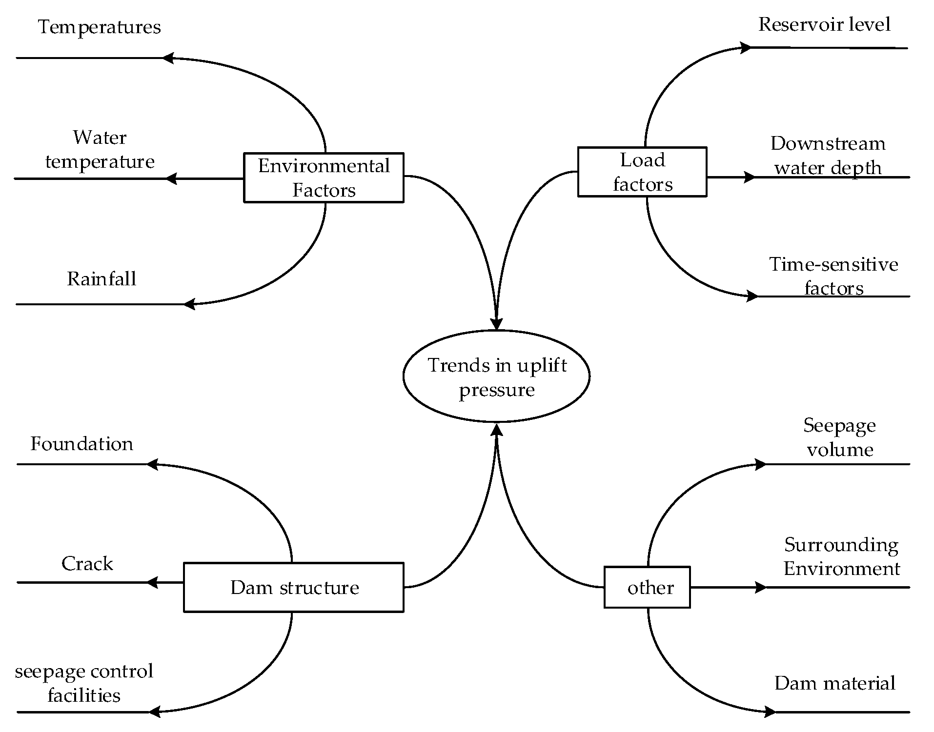
The change in uplift pressure is not only affected by environmental factors and load factors (reservoir level, temperature, rainfall, etc.) but it also depends on the dam’s own structure (permeability coefficient, cracks, seepage control facilities, etc.), as shown in Figure 1, making the pressure trend show nonlinear characteristics. Concrete dams often have a more complete online monitoring system. A large number of uplift pressure-monitoring samples have been collected by online dam monitoring systems. These rich data samples are critical for the establishment of a large sample monitoring model. In addition, the weak permeability of the dam material causes the change in water pressure in different parts of the dam base to lag behind the fluctuation in the reservoir level. Additional time intervals are required to fill or drain the porous media of the dam and the interior of the gauges, which results in a longer time for the gauges to reach a steady state of water. The above factors cause the time lag effect of the uplift pressure, which leads to a strong correlation between the uplift pressure values before and after the time series. In summary, the uplift pressure prediction model developed in this paper needs to solve a large-sample, time series, high-dimensional nonlinear problem.
2.2. Extraction of Uplift Pressure Features Based on the CNN Network
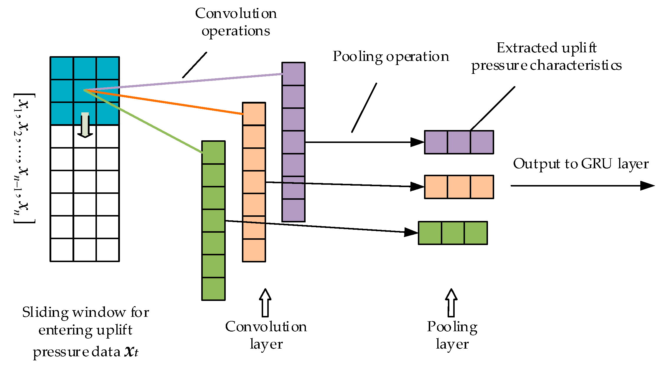
CNN is a feed-forward neural network that can be used to mine effective features from large amounts of dam safety monitoring data [18]. The CNN network structure is shown in Figure 2, which consists of a convolution layer, a pooling layer, and a fully connected layer. In this study, the hidden features in the dam monitoring data were first extracted by the convolution operation. Then, the data were downscaled by the pooling operation to reduce the dimensionality of the data as much as possible without changing the characteristics of the data. Finally, the extracted uplift pressure features were fed into the GRU neural network for learning. The expressions for the convolution and pooling operations are as follows:
Convolution operations:
where x is the input dataset, ω is the weight matrix, and t is the time.
Pooling operations:
where N denotes the length of the pooling operation area and is the output at the jth point of the kth group at the mth layer.
2.3. Prediction Model for Uplift Pressure Based on the GRU Network
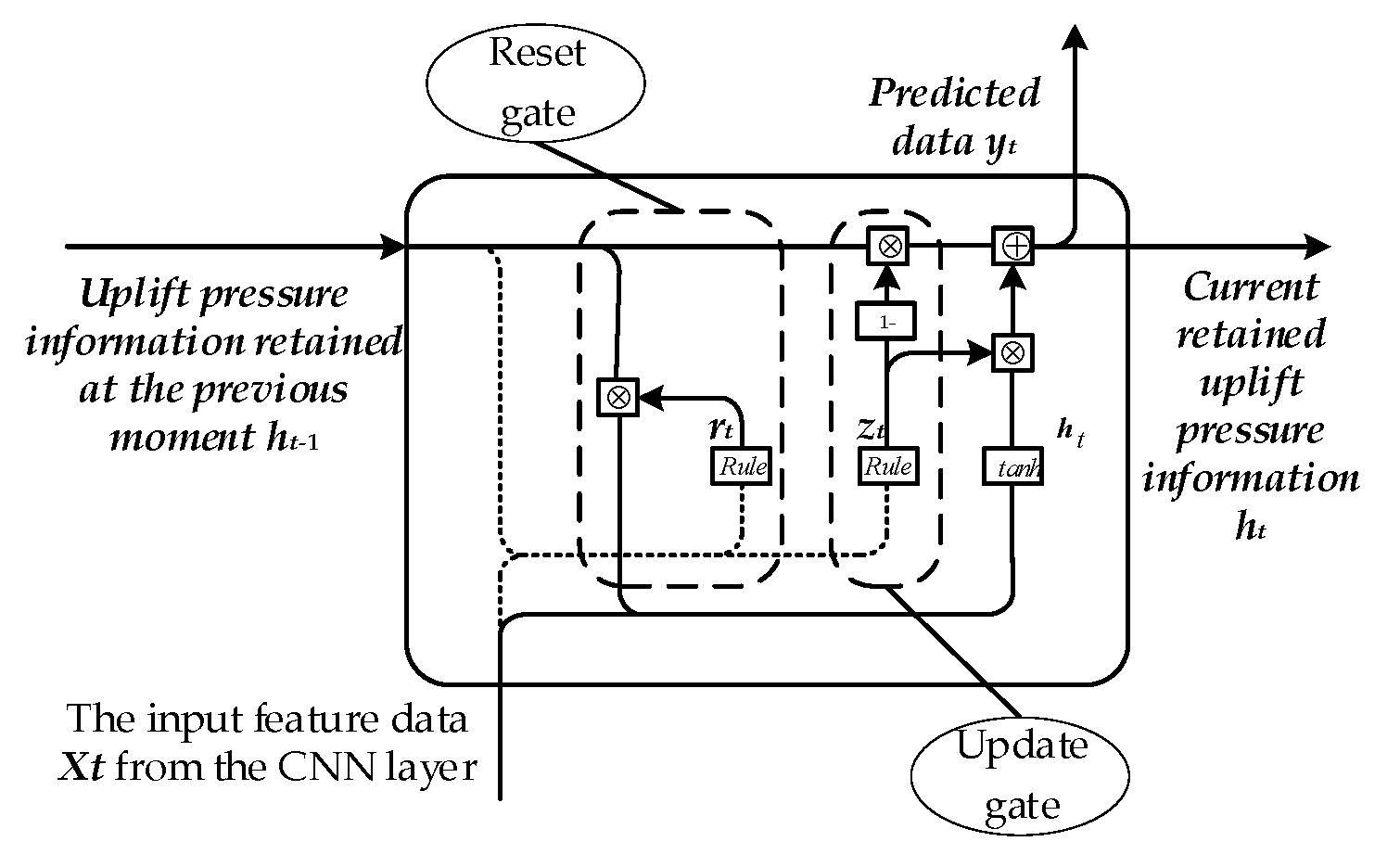
GRU is a performance-enhanced RNN variant with a long-term memory structure that allows temporal features in the data to be fully understood [19]. Furthermore, the GRU model is able to fit nonlinear features due to the nonlinear activation function (RULE activation function is used in this study). In this study, the GRU model was used to develop a mapping relationship between the uplift pressure and the environmental monitoring data of the concrete dam to predict the uplift pressure. The structure of the GRU unit is shown in Figure 3.
There are two gating structures in the GRU model prediction, the reset gate and the update gate, which are used to control the impact of the previous moment’s uplift pressure information on the current moment, thus fully learning the temporal characteristics of the uplift pressure data. The equations for the reset gate and update gate are as follows:
where refers to the output of the upper layer CNN network at moment t; is the uplift pressure information retained at moment t; is the uplift pressure information retained at moment t − 1; Wr and br are reset gate parameters; σ is the nonlinear activation function, where the rule activation function is chosen; and gr is the gating vector. Wz and bz are updated gate parameters; all parameters are automatically optimized by the backpropagation algorithm.
The propagation equations for the candidate hidden information at moment t and the retained uplift pressure information at moment t can be obtained from the equations of the update gate and the reset gate as follows:
This equation indicates that the updated amount of is controlled by both and .
2.4. Construction of the CNN-GRU Model for Uplift Pressure Prediction
The model simulation platform for this study is TensorFlow2.3, a deep learning framework under the Minconda3 configuration, and the script compilation language uses Python3.8. The concrete dam uplift pressure is affected by a variety of factors, such as water level and temperature. To correlate this characteristic information affecting the uplift pressure, the value of the uplift pressure at the same moment was represented as a vector in a series with the value of each factor, and the data were entered using a sliding window with a time sliding window designed in steps of 30 days. In this study, a CNN network was designed to extract effective features from uplift pressure-monitoring data samples. This network included 2 layers of convolution layers and 2 layers of pooling layers for better feature extraction. The GRU network was used to understand the feature vectors generated by the upper layer CNN network containing feature information. To improve the nonlinear computability of the GRU network structure and ultimately the model prediction capability, multiple GRU units were connected to form a chain-structured network. However, the multilayer GRU network structure inevitably exhibited exponential growth in parameters during the training process, which may affect the model prediction outcome. Therefore, the Adam optimization algorithm was used to update and optimize the model parameters [20]. The structure of the CNN-GRU uplift prediction model is presented in Figure 4, and the specific parameter settings are shown in Table 1.
The mean absolute error (MAE) was used as the optimized loss function of the CNN-GRU model, and the equations for the loss function are as follows:
where indicates the predicted value of uplift pressure; indicates the value of the uplift pressure monitoring.
2.5. Background of a Dam Project
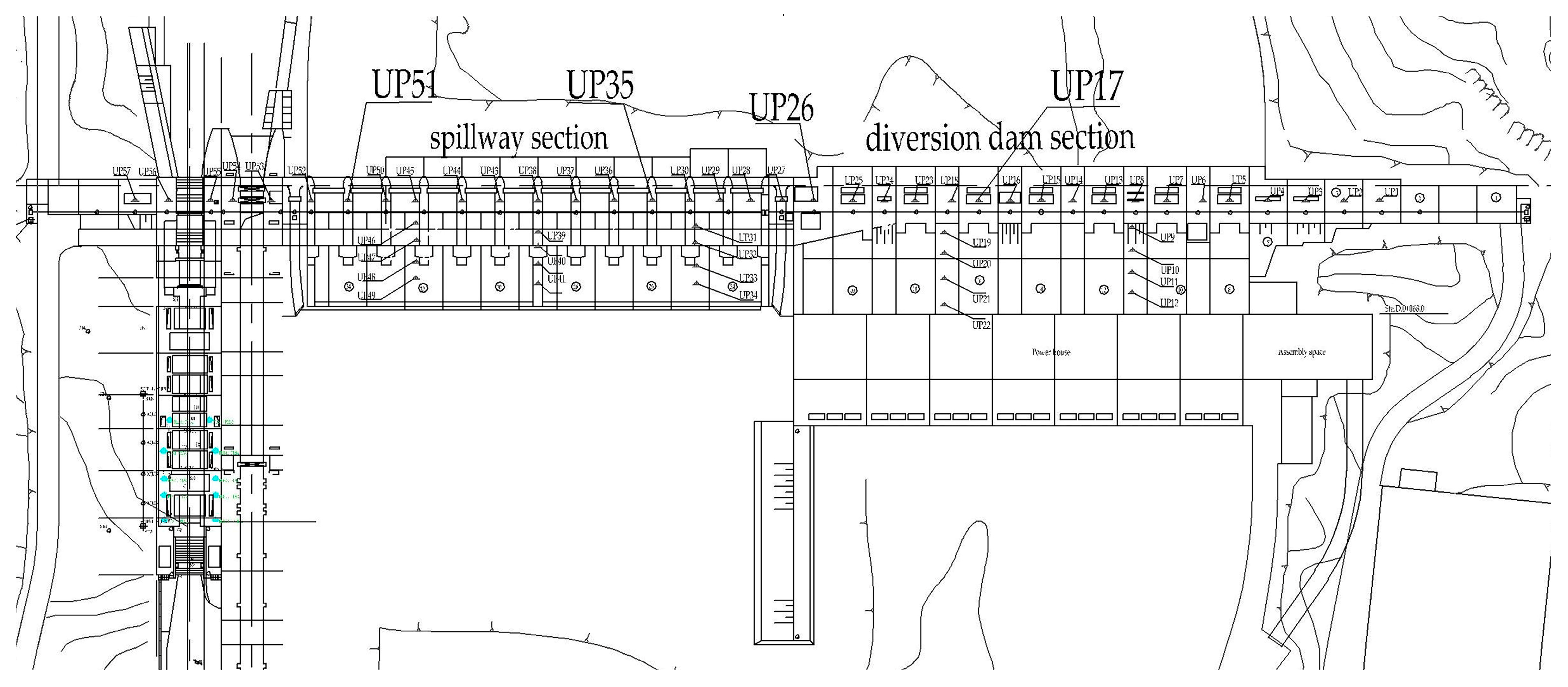
The dam uplift pressure of the Shuikou Hydropower Station project is predicted. The dam is a concrete gravity dam located on the main stream of the Minjiang River in the Fujian Province, China. The normal water level in front of the dam is 65.00 m, the flood limit water level is 61.00 m, the dead water level is 55.00 m, and the seismic precautionary intensity is Ⅶ. The dam has a total length of 783 m, a maximum height of 101 m, a maximum bottom length of 72 m, and a top elevation of 74 m. It consists of 42 dam sections, including the water blocking section, the power generation and diversion section, and the water discharge section. Table 2 shows the distribution of each dam section. Uplift pressure was monitored by a piezometer and a vibrating wire piezometer. Figure 5 illustrates the arrangement of uplift pressure measurement points. In this study, the uplift pressure-monitoring values of the four measuring points, UP17, UP26, UP35, and UP51, were selected as measuring points to verify the performance of the model. Figure 5 shows that UP17 and UP26 are in the diversion dam section and UP35 and UP51 are in the spillway dam section.
3. Results
3.1. Denoising of Uplift Pressure-Monitoring Data
There will be some noise in the uplift pressure-monitoring data due to aging electronic components, sensor induction distortion, signal channel disturbance, human factors, and other sudden abnormal factors. Real data mixed with noise will reduce the accuracy and stability of the prediction model. Therefore, the original data must be denoised to ensure validity of the data. Commonly used data denoising methods include the Kalman filter, Wiener filter, wavelet transform, empirical mode decomposition, etc. However, the Wiener filter and Kalman filter are not effective enough to address the problem of nonstationary sequence signals. The wavelet transform needs to set the basis function in advance during operation, and empirical mode decomposition is prone to spurious components and mode mixing during the decomposition of sequential signals. VMD overcomes the problems of mode mixing and spurious components of traditional methods and has been widely used in the field of data signal noise reduction [21,22,23,24].
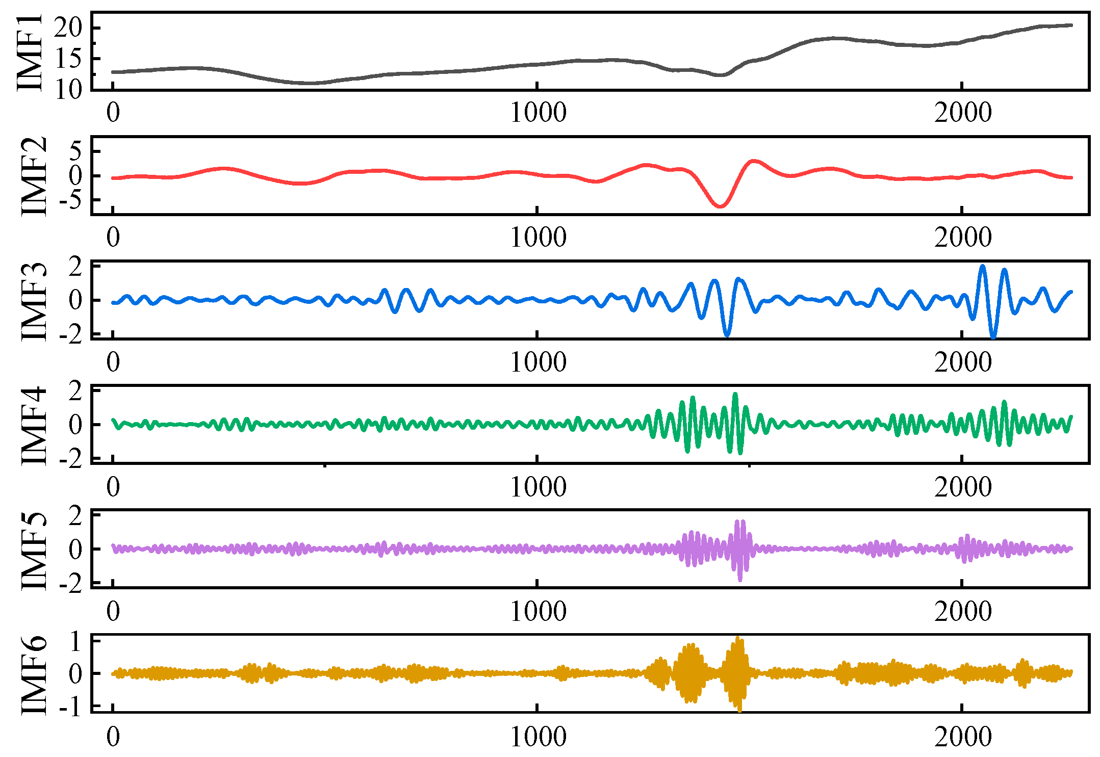
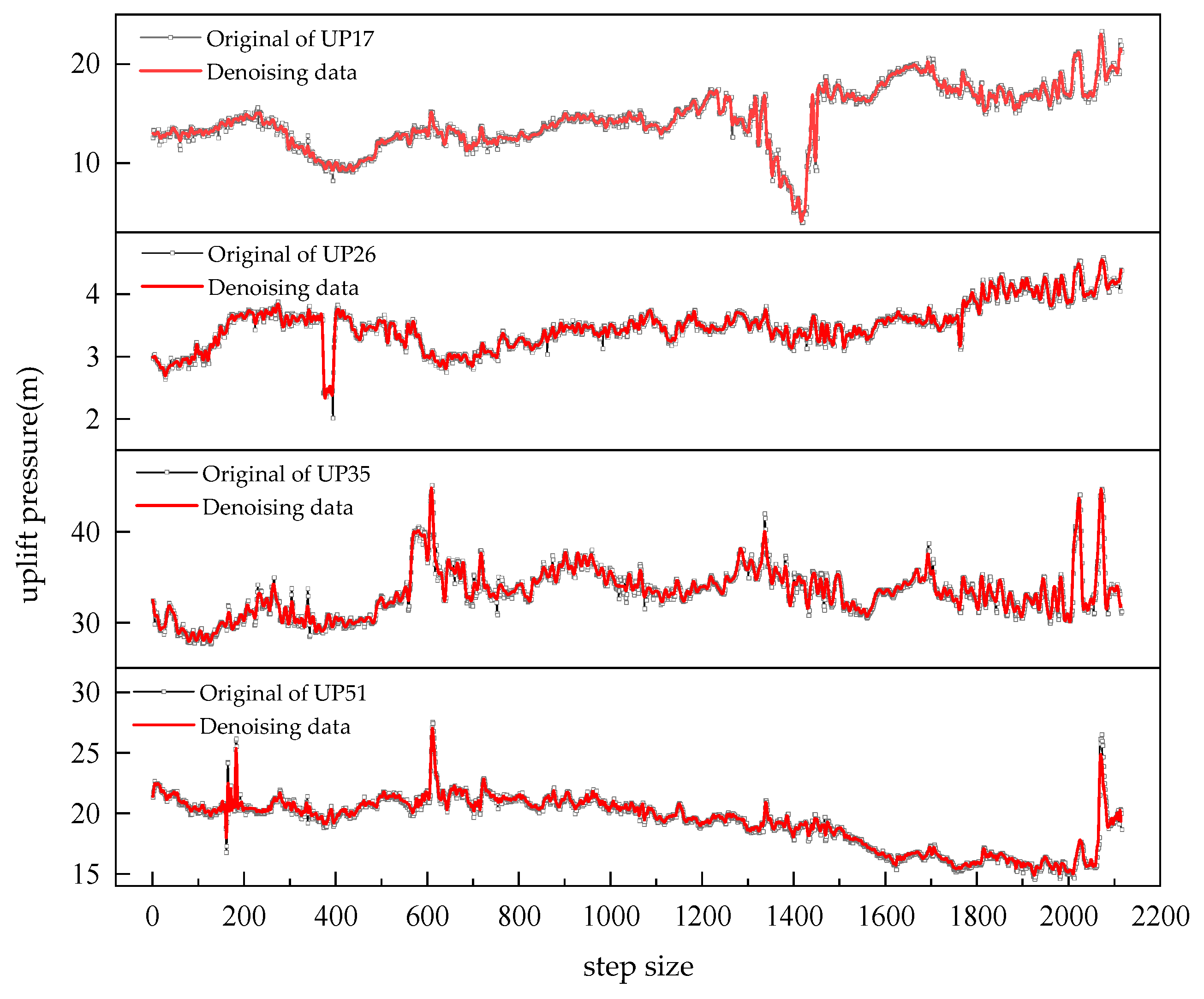
Therefore, VMD-SE was used to denoise the uplift pressure-monitoring data. The UP17 measurement point was used as an example. The monitored nonlinear, nonstationary historical uplift pressure data series was first decomposed into six intrinsic mode functions (IMFs) with gentle frequency changes and relative stability using variational modal decomposition (VMD). The VMD decomposition of the UP17 measurement point uplift pressure data is presented in Figure 6. Then, the noisy sequences were identified by calculating the value of sample entropy (SE) [25,26]. In this paper, the SE threshold was set to 0.5, i.e., sequences with SE values greater than 0.5 are noisy sequences. The SE values of each IMF component are presented in Table 3. IMF5 is a noisy sequence. Finally, the remaining IMF components are reconstituted to form the denoised data samples. A comparison of the denoised data samples with the original uplift pressure samples is shown in Figure 7.
3.2. Impact Factor and Input Data Set Analysis
In the case of a stable dam, the change in the uplift pressure of a concrete dam is mainly affected by upstream and downstream water levels, rainfall, temperature, and time effects [27]. The impact factors selected for this study include the following:
Water pressure component (HU, (HU)2, HU(2–3), HU(4–7), HU(8–15), HU(16–30), HU(31–60), HD), where HU denotes the upstream water level at the current monitoring date, HU(q-r) denotes the average upstream water level from q to r days before the current monitoring date and HD is the downstream water level at the current monitoring date; temperature component (T0–1, T2–7, T8–15, T16–30, T31–60, T61–120), where Tq-r denotes the average temperature from q to r days before the current monitoring date; rainfall component (R0–1, R2–3, R4–7, R8–15, R16–30, R31–60), where Rq-r denotes the cumulative value of rainfall from q to r days before the current monitoring date; time effects (θ, lnθ), where θ = t/100, t is the cumulative number of monitoring days from the observation date to the reference date.
The selection of input factors has an influential impact on the prediction accuracy of the model. Input factors with low correlation will not only increase the complexity of model iteration but also affect the accuracy of forecast results. Therefore, it is essential to select factors with substantial impacts. Since the Pearson correlation coefficient method has a large bias in dealing with nonlinear problems, the maximum information coefficient (MIC) is introduced in this paper to optimize the influence factors and determine the final set of input factors [28]. The results of the MIC calculations are presented in Table 4. It can be seen that the timing factor had a strong correlation with the uplift pressure, so it was retained; the water pressure component had a certain degree of correlation with the uplift pressure, and (HU(8–15), HU(16–30), HU(31–60), HD) were selected as input factors; the temperature component had a large MIC value, and (T16–30, T31–60, T61–120) were selected as input factors; the MIC values between rainfall components and uplift pressure were small and had limited effect on the trend of uplift pressure, so they were excluded. The final filtered input factors include: Water pressure component (HU(8–15), HU(16–30), HU(31–60), HD), Temperature component (T16–30, T31–60, T61–120), and Time effects (θ, lnθ).
In this study, the model reliability was validated by using the monitoring data of uplift pressure and the above environmental quantities from 4 July 2010 to 26 July 2016 as the input dataset. The data samples from 4 July 2010 to 11 May 2016 were used as training set samples to train the model, and the data samples from 12 May 2016 to 26 July 2016 were used as test samples to test the model performance effects.
3.3. Model Prediction
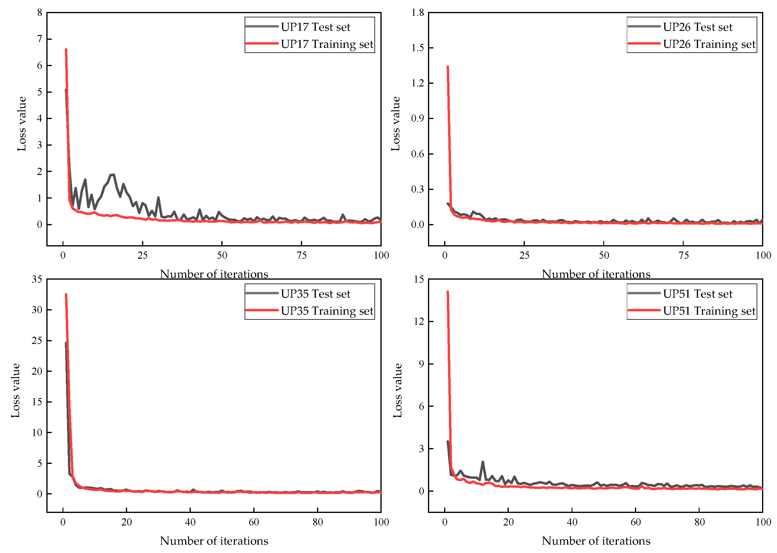
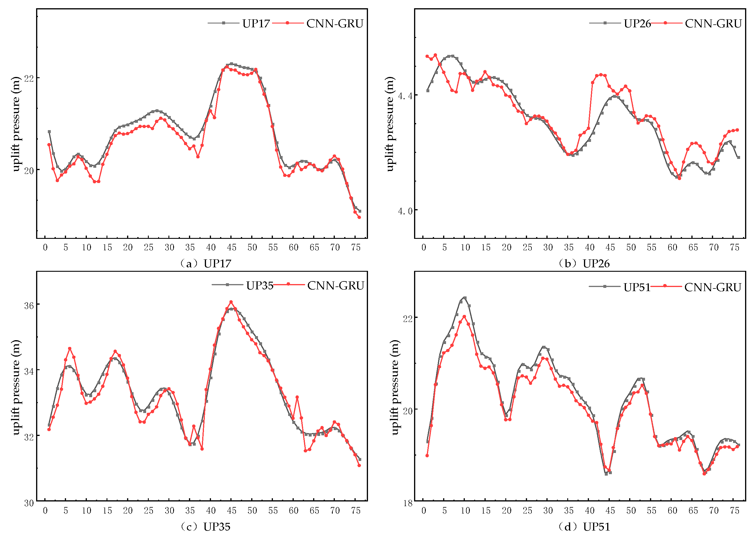
The denoised dataset was fed into the model, the model was trained using the training set, and then the model was tested using the test set. The iterative loss value curves for the model during training and prediction are shown in Figure 8, and the prediction results for the test set are shown in Figure 9.
4. Discussion
4.1. Analysis of the Denoising Effect of Uplift Pressure-Monitoring Data
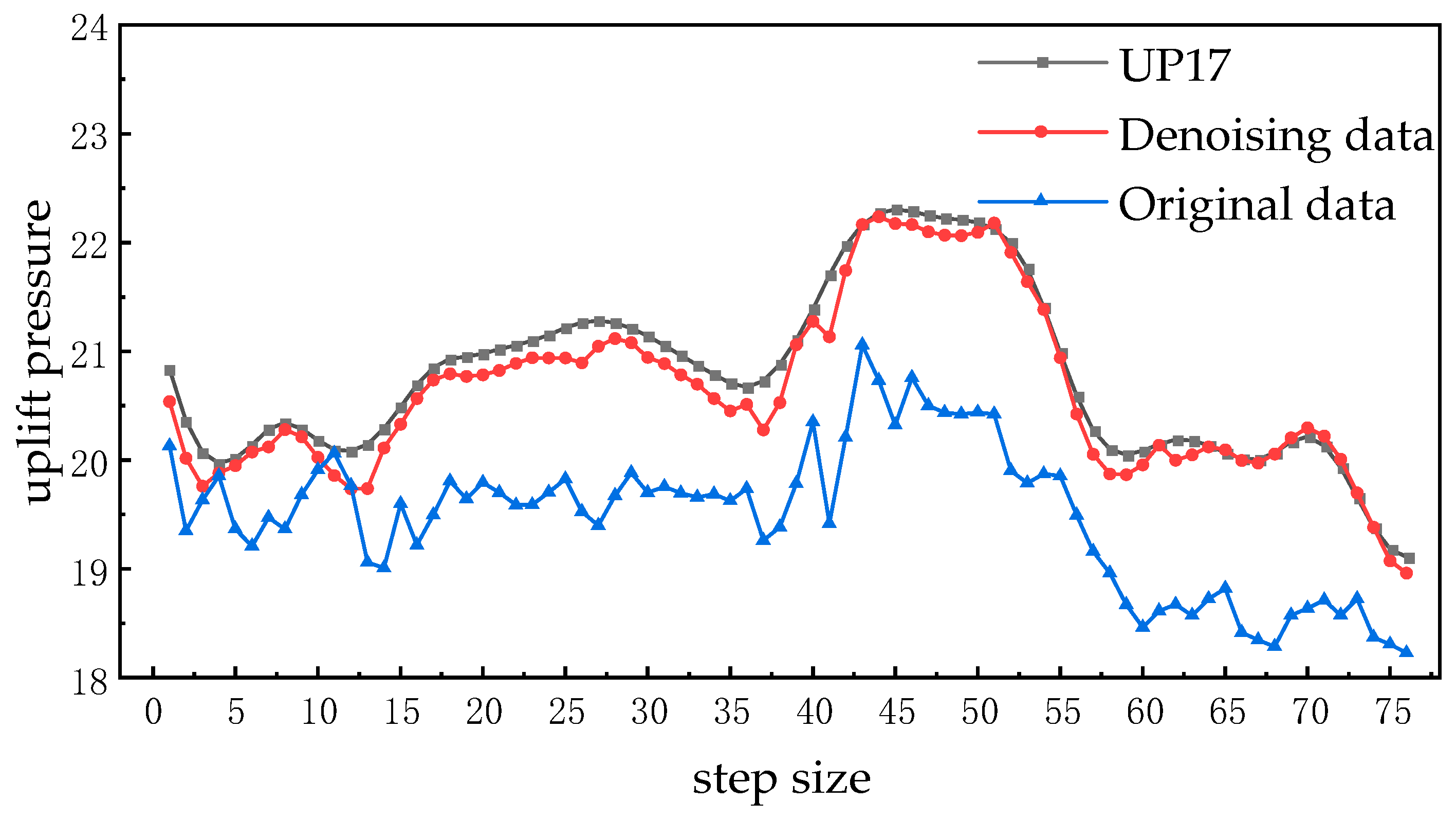
In the case of historical monitoring data directly used for prediction, a large error is generated due to the presence of noise sequences in the data. Therefore, the VMD-SE algorithm was employed to extract real information from the original data series to improve the accuracy of the uplift pressure prediction. To show the denoising effect of the method, a prediction model was established using the denoised data and the original monitoring data, and the root mean square error (RMSE) and mean absolute error (MAE) were used as evaluation indices, employing the UP17 measurement point as an example. The prediction results are shown in Figure 10, and the accuracy assessment is presented in Table 5.
According to Figure 10, when the original data were used for training and prediction, the volatility of the prediction results was greater; as seen in Table 5, the denoised data had considerably better RMSE and MAE than the original data, with reductions of 86.02% and 87.95%, respectively. The results showed that the VMD-SE algorithm can effectively filter out the noise and improve the model’s prediction results.
4.2. Analysis of the Uplift Pressure Prediction Results
As demonstrated in Figure 8, the CNN-GRU model had reasonable applicability on the training dataset, and the training loss curve exhibited a fast-decreasing trend. The model started to converge before 15 iterations and started to stabilize after 30 iterations; the final convergence was within the allowable error of all iterations. For the test process, the overall loss curve also showed a quickly decreasing trend within 30 iterations with a slightly higher convergence error at the end than in the training process. In conclusion, the CNN-GRU model performed well with regard to training and testing, indicating rationality in the network structure and parameter settings.
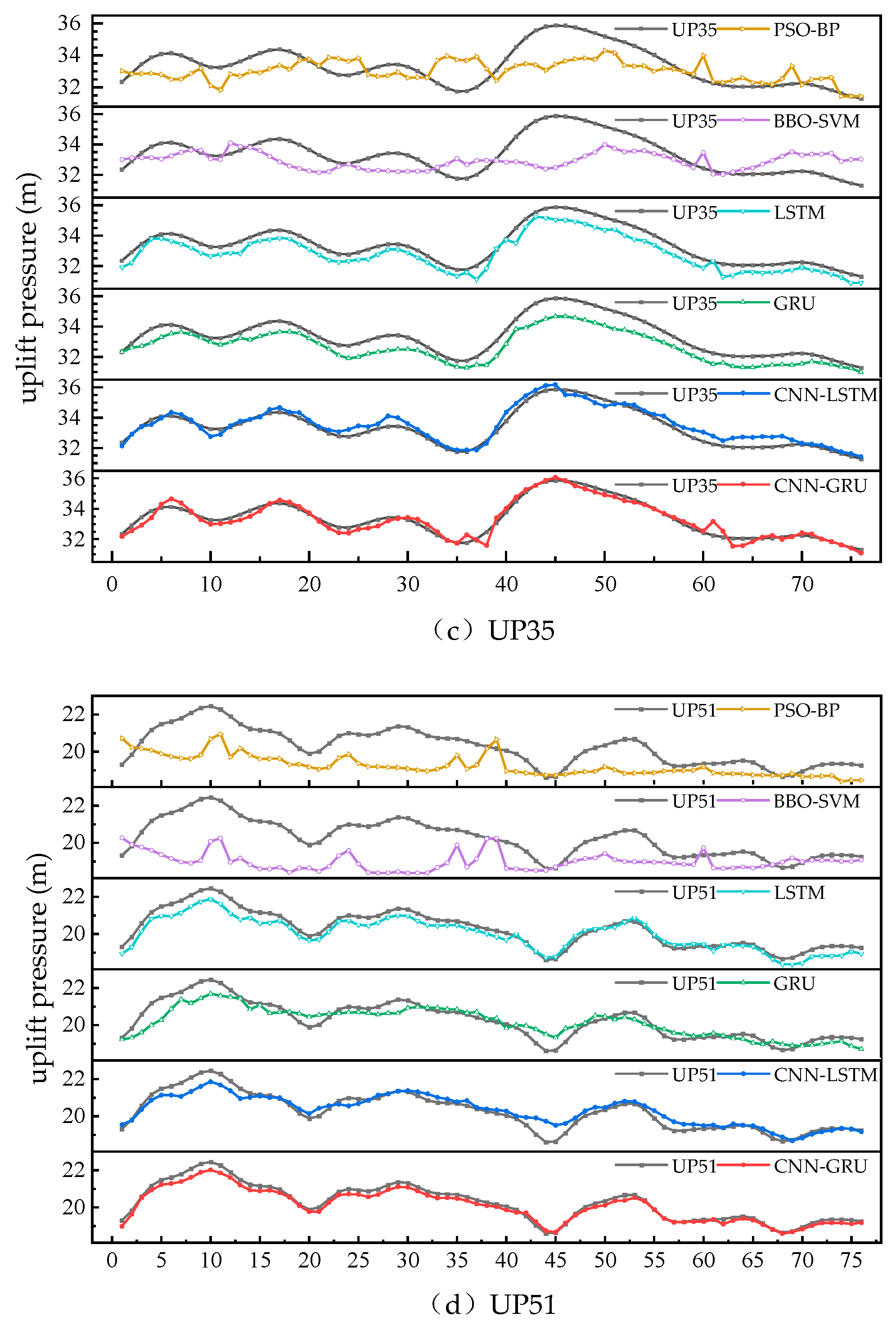
To demonstrate the advantages of the CNN-GRU model constructed in this paper in solving the large-sample time series uplift pressure prediction problem, the CNN-LSTM model, the GRU model, the LSTM model, the PSO-BP model, and the ABC-SVM model were compared against this model. The parameter settings of the deep learning model are consistent with those of the CNN-GRU model. The prediction results of each model on the uplift pressure data series of UP17, UP26, UP35, and UP51 measuring points are shown in Figure 11.
To measure the performance of the model more accurately, RMSE and MAE were selected as the evaluation indices of model prediction accuracy. In addition, to show the running efficiency of each model, the overall running time of each model was counted separately. The values of each evaluation index are shown in Table 6.
As demonstrated in Figure 11:
- (1)
- The BP and SVM causal models were considerably weaker than the deep learning models in terms of prediction performance, both in terms of overall trends and local inflection points.
- (2)
- The overall trend of the prediction curves of LSTM and GRU was basically the same as the monitoring value of the uplift pressure, but the trend of the prediction curve in the local inflection point area deviated from the monitoring curve, and the local inflection point could not be accurately predicted.
- (3)
- The fitting effect of the CNN-GRU model on the overall trend and local fluctuations was substantially better than that of the GRU model and the LSTM model, and it could more accurately describe the overall and local inflection points of the uplift pressure, and its prediction curve was closer to the monitoring curve of the uplift pressure.
- (4)
- The CNN-GRU model fits similarly to the CNN-LSTM model on the overall trend and local fluctuations at the UP26, UP35, and UP51 measurement points. However, the CNN-GRU model performs considerably better than the CNN-LSTM model at the UP17 measurement point.
Based on Table 6, the PSO-BP and ABC-SVM models had much larger RMSE and MAE evaluation indices than the other models, and it was clear that the LSTM, GRU, and CNN-GRU models, which considered historical uplift pressure time series characteristics, had a clear advantage over the PSO-BP and ABC-SVM models. Among them, the CNN-GRU model had a greater performance effect than the LSTM model and GRU model, which could be observed from the accuracy results. When the CNN-GRU was compared with the LSTM model and GRU model, the RMSE of the CNN-GRU model was reduced by 42.54%, 9.38%, 48.39%, 40%; 47.69%, 12.74%, 61.52%, 53%, and MAE was reduced by 32.70%, 7.31%, 56.52%, 40.27%; 53.21%, 6.56%, 66.90%, and 49.27%.
Although the evaluation metrics of the CNN-LSTM model are similar to those of the CNN-GRU model at the UP26, UP35, and UP51 measurement points, the evaluation metrics of the CNN-LSTM model are much larger than those of the CNN-GRU model and even larger than those of the GRU and LSTM models at the UP17 measurement point. The loss function curves of the CNN-LSTM model at the UP17 measurement point are presented in Figure 12. The training loss curve of the model is able to smooth out quickly. However, the test loss curve shows fluctuations, and the final value is much larger than the training loss value. This indicates that the model overfitted the prediction of UP17 measurement points.
Based on the results of this experiment, the following can be concluded:
- (1)
- Although causal models, such as BP and SVM, have reasonable prediction results for small sample data, they are unable to learn from data with time series characteristics, resulting in unsatisfactory prediction results for large sample data. In addition, the running time of the model in Table 6 shows that the running time of the SVM model increases exponentially when dealing with large sample data. This is because SVM usually uses the kernel matrix of the dataset to describe the similarity between samples, and when dealing with large sample data, the number of matrix elements increases squarely, resulting in unsatisfactory computational power and operational efficiency.
- (2)
- The LSTM model, GRU model, and CNN-GRU model, which consider the time series characteristics of historical uplift pressure-monitoring data, have obvious advantages over the PSO-BP model and ABC-SVM model. The performance of the LSTM model and GRU model is similar, but because the GRU model integrates the forget gate and input gate of the LSTM model into an update gate, which reduces the parameters required for training the GRU model [29], the training iteration of the GRU model is faster than that of the LSTM model with lower computational cost and higher operational efficiency.
- (3)
- The LSTM model and GRU model do not perform accurately enough on some of the measurement points with more fluctuations due to the inability to mine the potentially hidden information on the local fluctuation features of some of the measurement points. In contrast, CNN is able to extract the continuous and discontinuous features of sequence data and mine the variation characteristics of local fluctuation of uplift pressure, so the CNN-GRU model has better results compared with the LSTM model and GRU model.
- (4)
- The CNN-LSTM model predicts similarly to the CNN-GRU model, but because the model requires too many parameters to be trained and the amount of data is small, overfitting occurs at some prediction points, which makes the prediction results less than ideal.
In summary, all models can predict the trend of uplift pressure better, but the prediction performance of the deep learning model considering the correlation of time series data is superior compared with the general causal prediction model. The CNN-GRU and CNN-LSTM models constructed by the convolutional-cyclic idea can better describe the patterns of variations of the uplift pressure data series, but the CNN-LSTM model will be overfitted when the data volume is small due to the large number of parameters to be trained. The CNN-GRU model, on the other hand, not only has a higher iteration efficiency but also has a more accurate prediction effect on the overall trend, as well as local fluctuations at each measurement point.
The following limitations exist in this study:
- (1)
- The model proposed in this study has only been validated for uplift pressure prediction, and its suitability in different scenarios cannot be determined.
- (2)
- There are many hyperparameters involved in the model, and hyperparameters are adjustment knobs that control the structure, function, efficiency, and other functions of the model. These parameters basically have different settings in various scenarios, and currently, there are no uniform selection criteria, so they can only be determined by repeated trials in actual situations. Finding the optimal configuration of hyperparameters in these deep learning models in the high-dimensional data space involved in the field of dam safety monitoring is a major challenge and a difficulty to overcome in the future.
- (3)
- The model established in this study mainly focuses on individual measurement points for prediction while considering the time dimension of monitoring data, but each monitoring point of the dam will also be affected by the spatial dimension, i.e., the changing pattern of each monitoring point will be different under different spatial distribution locations. Therefore, determining the correlation links of each monitoring point of the dam in the spatial dimension, studying the variation law of each point under various spatial distributions, and establishing a dam safety prediction model with coupled spatio-temporal correlation characteristics are directions for future development.
5. Conclusions
- (1)
- In this study, the CNN-GRU model is proposed, in which the CNN network is used to extract potential connections and hidden information among the influencing factors of uplift pressure, and the GRU network is used to learn time series correlation features in the monitoring data for uplift pressure.
- (2)
- The CNN-GRU model was used to predict the uplift pressure data: MAE was 0.1554, 0.0398, 0.2306, and 0.1827. RMSE errors were 0.1903, 0.0548, 0.2916, and 0.2127.
- (3)
- In comparison with the CNN-LSTM, LSTM, GRU, PSO-BP, and ABC-SVM models, the CNN-GRU model constructed in this study has a better prediction effect on the overall trend and local fluctuation of the uplift pressure. Based on the accuracy assessment index, the model is more accurate than the other models, and the prediction curves are close to the surveillance data. The model can improve the utilization of dam safety monitoring results and has engineering practicality for safe dam operation.
Author Contributions
Conceptualization, G.H. and S.H.; Methodology, G.H. and S.H.; Software, G.H. and M.X.; Validation, G.H. and S.H.; Formal analysis, G.H.; Data curation, G.H. and M.X.; Writing—original draft preparation, G.H.; Writing—review and editing, G.H. and S.H.; Visualization, G.H.; Supervision, S.W. and S.H.; Funding acquisition, S.H. All authors have read and agreed to the published version of the manuscript.
Funding
The National Natural Science Foundation of China (42271026).
Data Availability Statement
Data cannot be made publicly available and readers should contact the corresponding author for details.
Conflicts of Interest
The authors declare no conflict of interest.
References
- Kalinina, A.; Spada, M.; Burgherr, P. Application of a Bayesian hierarchical modeling for risk assessment of accidents at hydropower dams. Saf. Sci. 2018, 110, 164–177. [Google Scholar] [CrossRef]
- Wen, Z.; Zhou, R.; Su, H. MR and stacked GRUs neural network combined model and its application for deformation prediction of concrete dam. Expert Syst. Appl. 2022, 201, 117272. [Google Scholar] [CrossRef]
- Ma, C.; Zhao, T.; Li, G.; Zhang, A.; Cheng, L. Intelligent Anomaly Identification of Uplift Pressure Monitoring Data and Structural Diagnosis of Concrete Dam. Appl. Sci. 2022, 12, 612. [Google Scholar] [CrossRef]
- Pereira, R.; Batista, A.L.; Neves, L.C.; Casaca, J.M. A priori uplift pressure model for concrete dam foundations based on piezometric monitoring data. Struct. Infrastruct. Eng. 2021, 17, 1523–1534. [Google Scholar] [CrossRef]
- Belmokre, A.; Mihoubi, M.K.; Santillan, D. Seepage and dam deformation analyses with statistical models: Support vector regression machine and random forest. In Proceedings of the 3rd International Conference on Structural Integrity, ICSI 2019, Funchal, Portugal, 2–5 September 2019; Volume 17, pp. 698–703. [Google Scholar] [CrossRef]
- Ishfaque, M.; Dai, Q.; Haq, N.u.; Jadoon, K.; Shahzad, S.M.; Janjuhah, H.T. Use of Recurrent Neural Network with Long Short-Term Memory for Seepage Prediction at Tarbela Dam, KP, Pakistan. Energies 2022, 15, 3123. [Google Scholar] [CrossRef]
- Salazar, F.; Toledo, M.A.; Oñate, E.; Morán, R. An empirical comparison of machine learning techniques for dam behaviour modelling. Struct. Saf. 2015, 56, 9–17. [Google Scholar] [CrossRef] [Green Version]
- Ranković, V.; Grujović, N.; Divac, D.; Milivojević, N. Development of support vector regression identification model for prediction of dam structural behaviour. Struct. Saf. 2014, 48, 33–39. [Google Scholar] [CrossRef]
- Su, H.; Li, X.; Yang, B.; Wen, Z. Wavelet support vector machine-based prediction model of dam deformation. Mech. Syst. Signal Proc. 2018, 110, 412–427. [Google Scholar] [CrossRef]
- Zhang, J.; Tang, H.; Tannant, D.D.; Lin, C.; Xia, D.; Liu, X.; Zhang, Y.; Ma, J. Combined forecasting model with CEEMD-LCSS reconstruction and the ABC-SVR method for landslide displacement prediction. J. Clean. Prod. 2021, 293, 126205. [Google Scholar] [CrossRef]
- Liu, H.-F.; Ren, C.; Zheng, Z.-T.; Liang, Y.-J.; Lu, X.-J. Study of a Gray Genetic BP Neural Network Model in Fault Monitoring and a Diagnosis System for Dam Safety. ISPRS Int. J. Geo-Inf. 2018, 7, 4. [Google Scholar] [CrossRef] [Green Version]
- Liu, Y.; Feng, X. Prediction of dam horizontal displacement based on CNN-LSTM and attention mechanism. Acad. J. Archit. Geotech. Eng. 2021, 3, 6. [Google Scholar] [CrossRef]
- Zhu, Y.; Gao, Y.; Wang, Z.; Cao, G.; Wang, R.; Lu, S.; Li, W.; Nie, W.; Zhang, Z. A Tailings Dam Long-Term Deformation Prediction Method Based on Empirical Mode Decomposition and LSTM Model Combined with Attention Mechanism. Water 2022, 14, 1229. [Google Scholar] [CrossRef]
- Cho, M.; Kim, C.; Jung, K.; Jung, H. Water Level Prediction Model Applying a Long Short-Term Memory (LSTM)–Gated Recurrent Unit (GRU) Method for Flood Prediction. Water 2022, 14, 2221. [Google Scholar] [CrossRef]
- Jia, P.; Zhang, H.; Liu, X.; Gong, X. Short-term photovoltaic power forecasting based on VMD and ISSA-GRU. IEEE Access 2021, 9, 105939–105950. [Google Scholar] [CrossRef]
- Yang, B.; Xiao, T.; Wang, L.; Huang, W. Using Complementary Ensemble Empirical Mode Decomposition and Gated Recurrent Unit to Predict Landslide Displacements in Dam Reservoir. Sensors 2022, 22, 1320. [Google Scholar] [CrossRef]
- Dai, Y.; Wang, Y.; Leng, M.; Yang, X.; Zhou, Q. LOWESS smoothing and Random Forest based GRU model: A short-term photovoltaic power generation forecasting method. Energy 2022, 256, 124661. [Google Scholar] [CrossRef]
- Wang, X.; Zhou, P.; Peng, X.; Wu, Z.; Yuan, H. Fault location of transmission line based on CNN-LSTM double-ended combined model. Energy Rep. 2022, 8, 781–791. [Google Scholar] [CrossRef]
- Li, W.; Logenthiran, T.; Woo, W.L. Multi-GRU prediction system for electricity generation’s planning and operation. IET Gener. Transm. Distrib. 2019, 13, 1630–1637. [Google Scholar] [CrossRef]
- Yi, D.; Ahn, J.; Ji, S. An Effective Optimization Method for Machine Learning Based on ADAM. Appl. Sci. 2020, 10, 1073. [Google Scholar] [CrossRef]
- Dragomiretskiy, K.; Zosso, D. Variational mode decomposition. IEEE Trans. Signal Process. 2013, 62, 531–544. [Google Scholar] [CrossRef]
- Lian, J.; Liu, Z.; Wang, H.; Dong, X. Adaptive variational mode decomposition method for signal processing based on mode characteristic. Mech. Syst. Signal Proc. 2018, 107, 53–77. [Google Scholar] [CrossRef]
- Li, F.; Ma, G.; Chen, S.; Huang, W. An ensemble modeling approach to forecast daily reservoir inflow using bidirectional long-and short-term memory (Bi-LSTM), variational mode decomposition (VMD), and energy entropy method. Water Resour. Manag. 2021, 35, 2941–2963. [Google Scholar] [CrossRef]
- Liu, Y.; Yang, G.; Li, M.; Yin, H. Variational mode decomposition denoising combined the detrended fluctuation analysis. Signal Process. 2016, 125, 349–364. [Google Scholar] [CrossRef]
- Wu, Q.; Lin, H. Daily urban air quality index forecasting based on variational mode decomposition, sample entropy and LSTM neural network. Sustain. Cities Soc. 2019, 50, 101657. [Google Scholar] [CrossRef]
- Wu, Y.; Zhang, D.N.; Yang, J.M.; Liu, Z.H. Short-term PV Power Prediction based on VMD-SE-TCAN Model. J. Comput. 2022, 33, 25–36. [Google Scholar] [CrossRef]
- Li, X.; Su, H.; Hu, J. The Prediction Model of Dam Uplift Pressure Based on Random Forest. In Proceedings of the IOP Conference Series: Materials Science and Engineering, Phuket, Thailand, 2–5 August 2017; Volume 229, p. 012025. [Google Scholar] [CrossRef] [Green Version]
- Lin, G.; Lin, A.; Gu, D. Using support vector regression and K-nearest neighbors for short-term traffic flow prediction based on maximal information coefficient. Inf. Sci. 2022, 608, 517–531. [Google Scholar] [CrossRef]
- Gao, S.; Huang, Y.; Zhang, S.; Han, J.; Wang, G.; Zhang, M.; Lin, Q. Short-term runoff prediction with GRU and LSTM networks without requiring time step optimization during sample generation. J. Hydrol. 2020, 589, 125188. [Google Scholar] [CrossRef]
Figure 1.
Factors affecting the amount of dam uplift pressure effect.

Figure 2.
The CNN network structure.

Figure 3.
The internal structure of GRU unit.

Figure 4.
The structure of the CNN-GRU uplift prediction model.

Figure 5.
The arrangement of uplift pressure measurement points.

Figure 6.
The VMD decomposition of the UP17 measurement point.

Figure 7.
The comparison between the denoised data samples and the original uplift pressure data samples.
Figure 7.
The comparison between the denoised data samples and the original uplift pressure data samples.

Figure 8.
Iterative loss value curve.

Figure 9.
Uplift pressure predicted results. ((a): Prediction results of CNN-GRU model in the UP17 measurement point; (b): Prediction results of CNN-GRU model in the UP26 measurement point; (c): Prediction results of CNN-GRU model in the UP35 measurement point; (d): Prediction results of CNN-GRU model in the UP51 measurement point.)

Figure 10.
Prediction curves for the original and denoised data of UP17 measurement points.

Figure 11.
Comparison of uplift pressure prediction results. ((a): The prediction results of each model on the uplift pressure data of the UP17 measuring point; (b): The prediction results of each model on the uplift pressure data of the UP26 measuring point; (c): The prediction results of each model on the uplift pressure data of the UP35 measuring point; (d): The prediction results of each model on the uplift pressure data of the UP51 measuring point.)


Figure 12.
Loss function of the CNN-LSTM model at UP17 measurement points.


Table 1.
CNN-GRU model parameter setting.
| Network Structure | Experimental Parameters | Parameter Value |
|---|---|---|
| Overall Structure | optimization algorithm | Adam |
| batch size | 128 | |
| epochs | 100 | |
| CNN structure (2 layers) | convolution kernels | 16, 32 |
| kernel size | 2 | |
| strides | 2 | |
| activation | ||
| pool size | 2 | |
| strides | 2 | |
| GRU structure (3 layers) | hidden neurons | 64, 64, 64 |
| dropout | 0.2 | |
| activation | ||
| Fully connected layer (1 layer) | units | 1 |
| activation | None |
Table 2.
The distribution of each dam section.
| Dam Section | Left Bank Water Blocking Section | Diversion Section | Discharge Section | Spillway Section | Bottom Outlet Section | Ship Lock | Right -Shore Water Blocking Section |
|---|---|---|---|---|---|---|---|
| Number | 1#~7# | 8#~21# | 22# | 23#~35# | 36# | 37#~38# | 39#~42# |
Table 3.
The sample entropy values of the UP17 measurement point.
| Subsequences | IMF1 | IMF2 | IMF3 | IMF4 | IMF5 | IMF6 |
|---|---|---|---|---|---|---|
| SE | 0.0111 | 0.0438 | 0.2094 | 0.4050 | 0.5324 | 0.4856 |
Table 4.
Impact factor preference.
| Component Name | Factors | Whether to Be Selected | |
|---|---|---|---|
| Time effects | θ | 0.8995 | Y |
| lnθ | 0.8995 | Y | |
| Water pressure component | HU | 0.1945 | N |
| (HU)2 | 0.1945 | N | |
| HU(2–3) | 0.2078 | N | |
| HU(4–7) | 0.2175 | N | |
| H(U8–15) | 0.2487 | Y | |
| HU(16–30) | 0.2675 | Y | |
| HU(31–60) | 0.2537 | Y | |
| HD | 0.2451 | Y | |
| Temperature component | T0–1 | 0.4725 | N |
| T2–7 | 0.5147 | N | |
| T8–15 | 0.5253 | N | |
| T16–30 | 0.6071 | Y | |
| T31–60 | 0.6064 | Y | |
| T61–120 | 0.7076 | Y | |
| Rainfall component | R0–1 | 0.1908 | N |
| R2–3 | 0.1562 | N | |
| R4–7 | 0.1723 | N | |
| R8–15 | 0.1804 | N | |
| R16–30 | 0.1912 | N | |
| R31–60 | 0.1984 | N |
Table 5.
Statistics of prediction evaluation indexes for original and denoised data of UP17 measurement points.
Table 5.
Statistics of prediction evaluation indexes for original and denoised data of UP17 measurement points.
| UP17 | RMSE | MAE |
|---|---|---|
| Original data | 1.3614 | 1.2890 |
| denoised data | 0.1903 | 0.1554 |
Table 6.
The value of each evaluation index.
| Points | UP17 | UP26 | ||||
| Models | RMSE/(m) | MAE/(m) | Time/s | RMSE/(m) | MAE/(m) | Time/s |
| LSTM | 0.3312 | 0.2309 | 325.12 | 0.0605 | 0.0429 | 353.95 |
| GRU | 0.3638 | 0.3321 | 199.23 | 0.0629 | 0.0426 | 277.76 |
| CNN-GRU | 0.1903 | 0.1554 | 276.38 | 0.0548 | 0.0398 | 291.83 |
| PSO-BP | 1.0973 | 0.8919 | 215.43 | 0.1674 | 0.1416 | 212.69 |
| ABC-SVM | 1.0165 | 0.8303 | 464.51 | 0.1438 | 0.1225 | 582.21 |
| Points | UP35 | UP51 | ||||
| Models | RMSE/(m) | MAE/(m) | Time/s | RMSE/(m) | MAE/(m) | Time/s |
| LSTM | 0.5650 | 0.5305 | 382.02 | 0.3549 | 0.3059 | 321.54 |
| GRU | 0.7577 | 0.6967 | 300.28 | 0.4484 | 0.3602 | 183.03 |
| CNN-GRU | 0.2916 | 0.2306 | 310.53 | 0.2127 | 0.1827 | 222.77 |
| PSO-BP | 1.1081 | 0.8951 | 154.85 | 1.2607 | 1.0787 | 186 |
| ABC-SVM | 1.2673 | 0.9972 | 569.27 | 1.6306 | 1.3256 | 523.13 |
Disclaimer/Publisher’s Note: The statements, opinions and data contained in all publications are solely those of the individual author(s) and contributor(s) and not of MDPI and/or the editor(s). MDPI and/or the editor(s) disclaim responsibility for any injury to people or property resulting from any ideas, methods, instructions or products referred to in the content. |
© 2023 by the authors. Licensee MDPI, Basel, Switzerland. This article is an open access article distributed under the terms and conditions of the Creative Commons Attribution (CC BY) license (https://creativecommons.org/licenses/by/4.0/).
Share and Cite
MDPI and ACS Style
Hua, G.; Wang, S.; Xiao, M.; Hu, S. Research on the Uplift Pressure Prediction of Concrete Dams Based on the CNN-GRU Model. Water 2023, 15, 319. https://doi.org/10.3390/w15020319
AMA Style
Hua G, Wang S, Xiao M, Hu S. Research on the Uplift Pressure Prediction of Concrete Dams Based on the CNN-GRU Model. Water. 2023; 15(2):319. https://doi.org/10.3390/w15020319
Chicago/Turabian StyleHua, Guowei, Shijie Wang, Meng Xiao, and Shaohua Hu. 2023. "Research on the Uplift Pressure Prediction of Concrete Dams Based on the CNN-GRU Model" Water 15, no. 2: 319. https://doi.org/10.3390/w15020319
Note that from the first issue of 2016, this journal uses article numbers instead of page numbers. See further details here.