
Retrieving Eutrophic Water in Highly Urbanized Area Coupling UAV Multispectral Data and Machine Learning Algorithms
 , and
, and
Abstract
:1. Introduction
2. Materials and Methods
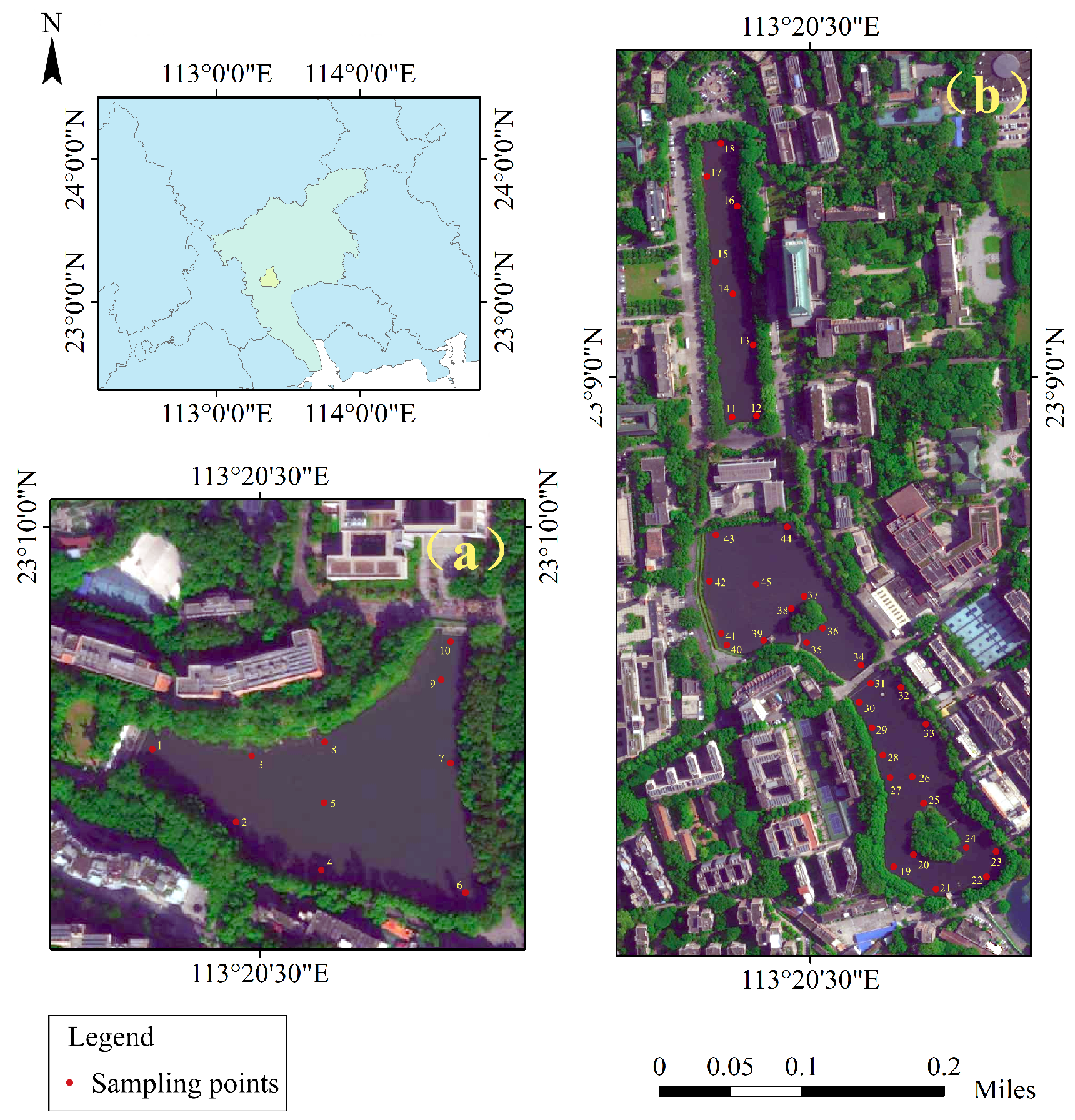
2.1. Study Area
2.2. Data Collection
2.2.1. Field Data
2.2.2. UAV Data
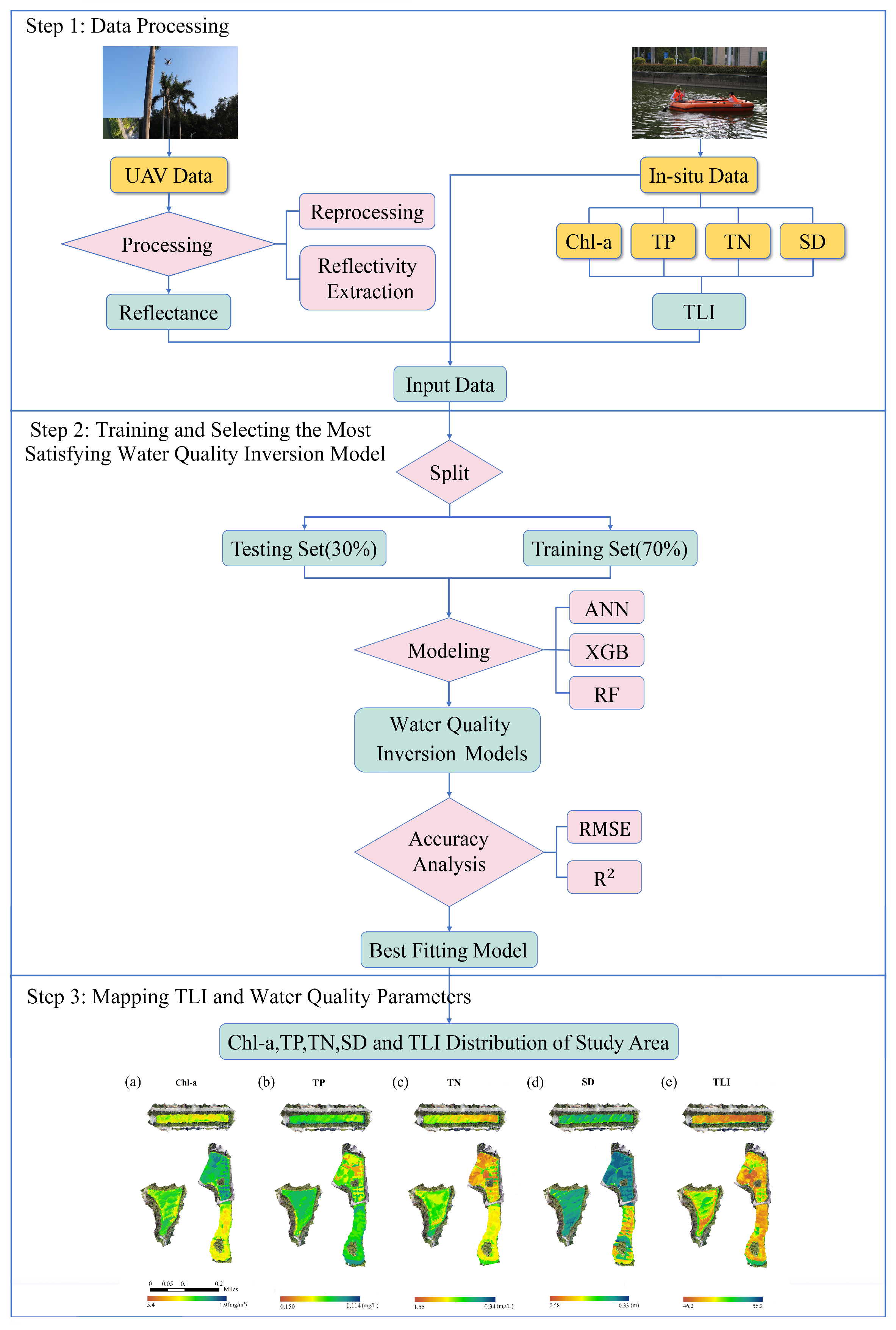
2.3. Method
2.3.1. Data Processing
2.3.2. Quantification of Trophic State
2.3.3. Modeling Approaches
3. Result
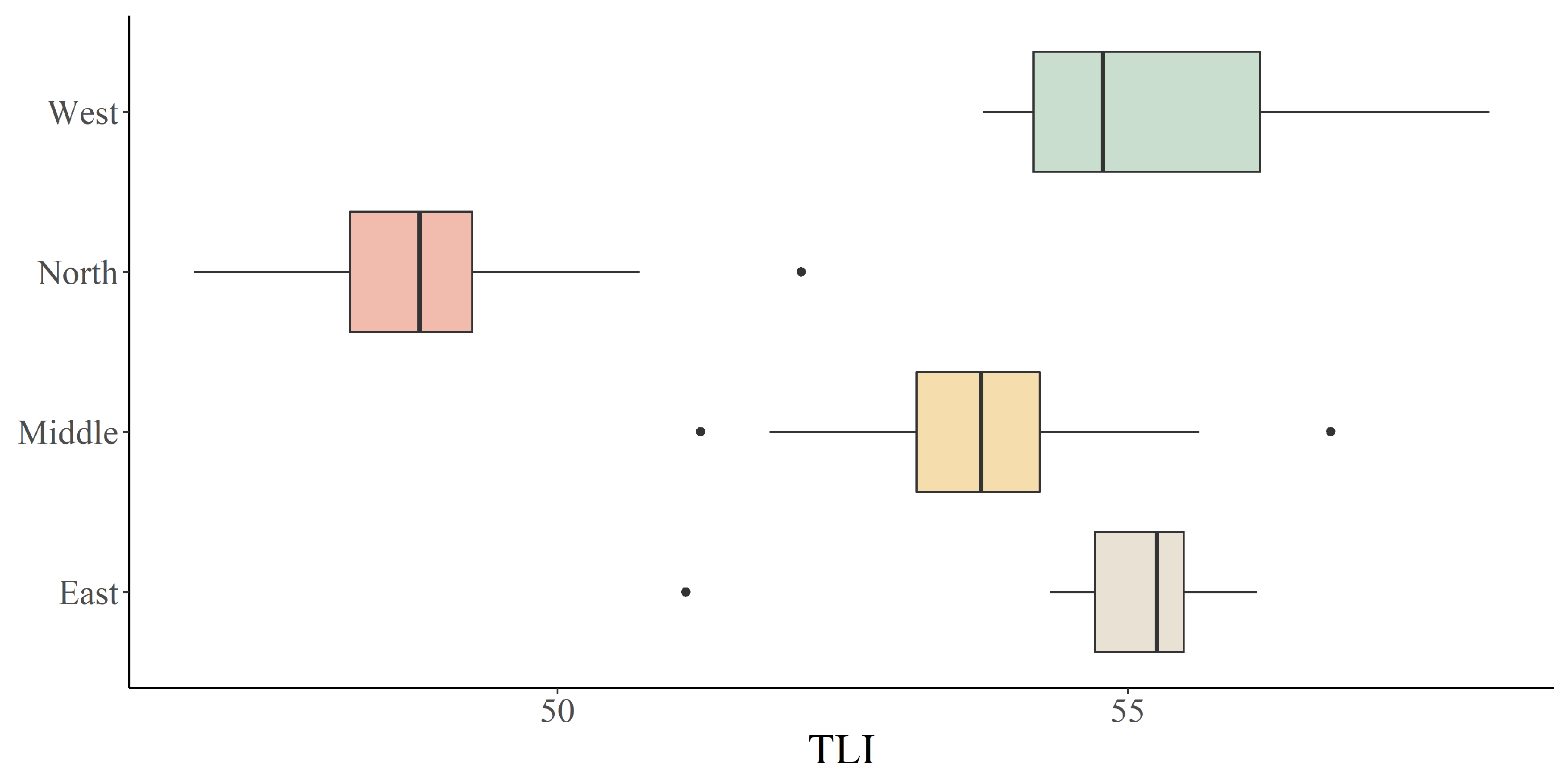
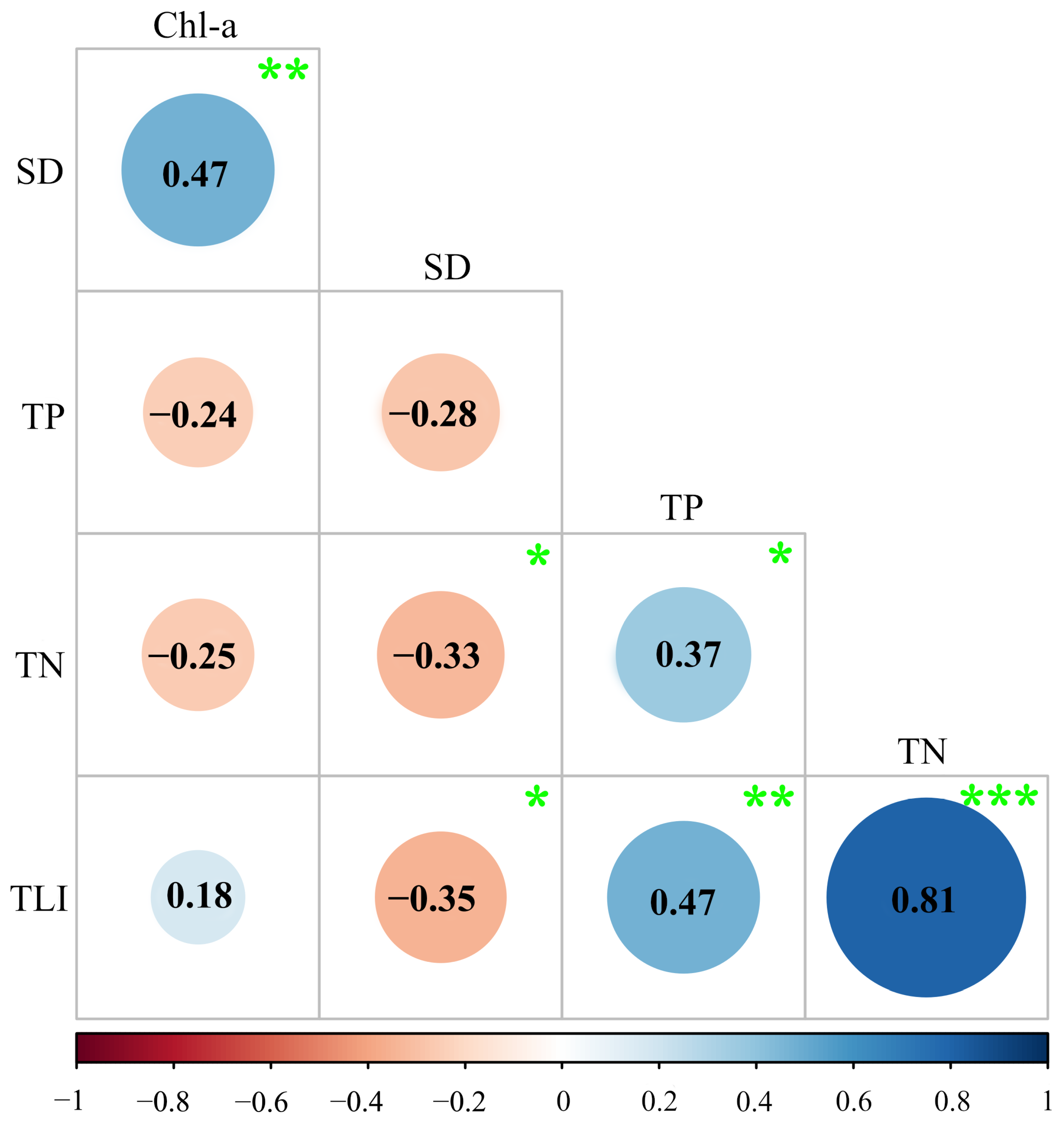
3.1. Measured Data Analysis and TLI Level
3.2. Model Accuracy Verification and Comparison
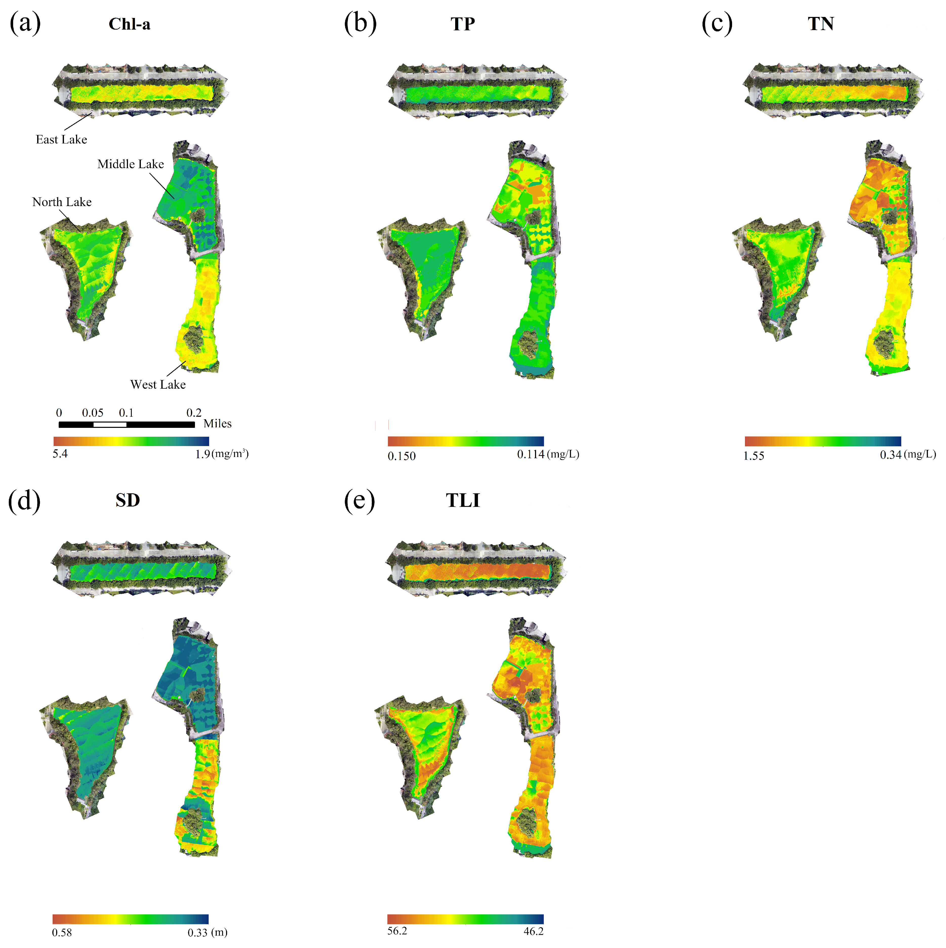
3.3. Spatial Distribution of Water Quality and Eutrophication Degree
4. Discussion
5. Conclusions
Author Contributions
Funding
Data Availability Statement
Acknowledgments
Conflicts of Interest
Appendix A

| Sampling Point | Chl-a | TP | TN | SD |
|---|---|---|---|---|
| 1 | 4.62 | 0.139 | 0.421 | 0.4 |
| 2 | 4.6 | 0.103 | 0.262 | 0.42 |
| 3 | 4.39 | 0.105 | 0.152 | 0.43 |
| 4 | 3.01 | 0.099 | 0.315 | 0.38 |
| 5 | 3.56 | 0.098 | 0.246 | 0.44 |
| 6 | 2.54 | 0.125 | 0.315 | 0.4 |
| 7 | 2.24 | 0.11 | 0.345 | 0.39 |
| 8 | 3.4 | 0.115 | 0.296 | 0.4 |
| 9 | 2.77 | 0.146 | 0.318 | 0.3 |
| 10 | 2.46 | 0.122 | 0.41 | 0.4 |
| 11 | 2.43 | 0.141 | 0.583 | 0.4 |
| 12 | 5.4 | 0.116 | 0.899 | 0.45 |
| 13 | 5.99 | 0.11 | 0.912 | 0.42 |
| 14 | 5.27 | 0.142 | 0.823 | 0.4 |
| 15 | 5.67 | 0.115 | 1.05 | 0.42 |
| 16 | 3.28 | 0.125 | 1.45 | 0.37 |
| 17 | 2.16 | 0.153 | 1.88 | 0.38 |
| 18 | 4.72 | 0.139 | 1.21 | 0.4 |
| 19 | 5.2 | 0.13 | 0.865 | 0.78 |
| 20 | 3.71 | 0.123 | 0.955 | 0.38 |
| 21 | 5.48 | 0.124 | 0.835 | 0.52 |
| 22 | 6.26 | 0.116 | 1.09 | 0.34 |
| 23 | 2.74 | 0.115 | 1.02 | 0.36 |
| 24 | 4.79 | 0.122 | 1 | 0.4 |
| 25 | 3.3 | 0.181 | 0.654 | 0.37 |
| 26 | 4.82 | 0.117 | 0.896 | 0.48 |
| 27 | 3.42 | 0.117 | 1.05 | 0.37 |
| 28 | 4.3 | 0.112 | 1.35 | 0.38 |
| 29 | 2.39 | 0.116 | 0.956 | 0.43 |
| 30 | 1.74 | 0.114 | 1.18 | 0.45 |
| 31 | 2.69 | 0.136 | 0.955 | 0.4 |
| 32 | 4.43 | 0.111 | 0.756 | 0.42 |
| 33 | 5.61 | 0.116 | 0.815 | 0.43 |
| 34 | 1.82 | 0.14 | 1.56 | 0.4 |
| 35 | 1.72 | 0.134 | 1.48 | 0.26 |
| 36 | 3.88 | 0.139 | 1.42 | 0.3 |
| 37 | 2.64 | 0.133 | 1.65 | 0.26 |
| 38 | 3.05 | 0.145 | 1.04 | 0.27 |
| 39 | 3.74 | 0.123 | 0.8 | 0.28 |
| 40 | 2.06 | 0.127 | 1.25 | 0.27 |
| 41 | 3.12 | 0.168 | 1.62 | 0.27 |
| 42 | 3.05 | 0.13 | 0.802 | 0.29 |
| 43 | 1.26 | 0.132 | 1.62 | 0.27 |
| 44 | 2.04 | 0.12 | 1.58 | 0.34 |
| 45 | 1.73 | 0.127 | 1.19 | 0.27 |
References
- Smith, V.H.; Schindler, D.W. Eutrophication science: Where do we go from here? Trends Ecol. Evol. 2009, 24, 201–207. [Google Scholar] [CrossRef]
- Matthews, M.W.; Bernard, S. Eutrophication and cyanobacteria in South Africa’s standing water bodies: A view from space. S. Afr. J. Sci. 2015, 111, 7. [Google Scholar] [CrossRef] [Green Version]
- Smith, V.H.; Joye, S.B.; Howarth, R.W. Eutrophication of freshwater and marine ecosystems. Limnol. Oceanogr. 2006, 51, 351–355. [Google Scholar] [CrossRef] [Green Version]
- Nazari-Sharabian, M.; Taheriyoun, M. Climate change impact on water quality in the integrated Mahabad Dam watershed-reservoir system. J. Hydro Environ. Res. 2021, 40, 28–37. [Google Scholar] [CrossRef]
- Guan, Q.; Feng, L.; Hou, X.; Schurgers, G.; Zheng, Y.; Tang, J. Eutrophication changes in fifty large lakes on the Yangtze Plain of China derived from MERIS and OLCI observations. Remote Sens. Environ. 2020, 246, 111890. [Google Scholar] [CrossRef]
- Ke, S.; Zhang, P.; Ou, S.; Zhang, J.; Chen, J.; Zhang, J. Spatiotemporal nutrient patterns, composition, and implications for eutrophication mitigation in the Pearl River Estuary, China. Estuar. Coast. Shelf Sci. 2022, 266, 107749. [Google Scholar] [CrossRef]
- Huang, X.; Huang, L.; Yue, W. The characteristics of nutrients and eutrophication in the Pearl River estuary, South China. Mar. Pollut. Bull. 2003, 47, 30–36. [Google Scholar] [CrossRef]
- Ministry of Ecology and Environment. China Ecological and Environmental Bulletin 2019; Ministry of Ecology and Environment in China, 15 December 2019. Available online: https://www.mee.gov.cn/xxgk2018/xxgk/xxgk15/202005/t20200507_777895.html (accessed on 7 May 2020). (In Chinese)
- Schindler, D.W. Recent advances in the understanding and management of eutrophication. Limnol. Oceanogr. 2006, 51, 356–363. [Google Scholar] [CrossRef] [Green Version]
- Yang, Y.; Bai, Y.; Wang, X.; Wang, L.; Jin, X.; Sun, Q. Group Decision-Making Support for Sustainable Governance of Algal Bloom in Urban Lakes. Sustainability 2020, 12, 1494. [Google Scholar] [CrossRef] [Green Version]
- Sharabian, M.N.; Ahmad, S.; Karakouzian, M. Climate Change and Eutrophication: A Short Review. Eng. Technol. Appl. Sci. Res. 2018, 8, 3668–3672. [Google Scholar] [CrossRef]
- Gholizadeh, M.H.; Melesse, A.M.; Reddi, L. A Comprehensive Review on Water Quality Parameters Estimation Using Remote Sensing Techniques. Sensors 2016, 16, 1298. [Google Scholar] [CrossRef] [PubMed] [Green Version]
- Verma, S. Wireless Sensor Network Application for Water Quality Monitoring in India. In Proceedings of the 2012 National Conference on Computing and Communication Systems, Durgapur, India, 21–22 November 2012; IEEE: Piscataway, NJ, USA, 2012; pp. 1–5. [Google Scholar]
- Adu-Manu, K.S.; Katsriku, F.A.; Abdulai, J.-D.; Engmann, F. Smart River Monitoring Using Wireless Sensor Networks. Wirel. Commun. Mob. Comput. 2020, 2020, 1–19. [Google Scholar] [CrossRef]
- Park, J.; Kim, K.T.; Lee, W.H. Recent Advances in Information and Communications Technology (ICT) and Sensor Technology for Monitoring Water Quality. Water 2020, 12, 510. [Google Scholar] [CrossRef] [Green Version]
- Robarts, R.D.; Barker, S.J.; Evans, S. Water Quality Monitoring and Assessment: Current Status and Future Needs. In Proceedings of the 12th World Lake Conference, Jaipur, Rajasthan, India, 28 October–2 November 2007. [Google Scholar]
- Cheng, K.-S.; Lei, T.-C. Reservoir Trophic State Evaluation Using Lanisat Tm Images. JAWRA J. Am. Water Resour. Assoc. 2001, 37, 1321–1334. [Google Scholar] [CrossRef]
- Mamun, M.; Ferdous, J.; An, K.-G. Empirical Estimation of Nutrient, Organic Matter and Algal Chlorophyll in a Drinking Water Reservoir Using Landsat 5 TM Data. Remote Sens. 2021, 13, 2256. [Google Scholar] [CrossRef]
- Shi, J.; Shen, Q.; Yao, Y.; Li, J.; Chen, F.; Wang, R.; Xu, W.; Gao, Z.; Wang, L.; Zhou, Y. Estimation of Chlorophyll-a Concentrations in Small Water Bodies: Comparison of Fused Gaofen-6 and Sentinel-2 Sensors. Remote Sens. 2022, 14, 229. [Google Scholar] [CrossRef]
- Soomets, T.; Uudeberg, K.; Jakovels, D.; Brauns, A.; Zagars, M.; Kutser, T. Validation and Comparison of Water Quality Products in Baltic Lakes Using Sentinel-2 MSI and Sentinel-3 OLCI Data. Sensors 2020, 20, 742. [Google Scholar] [CrossRef] [Green Version]
- Cao, Z.; Ma, R.; Duan, H.; Pahlevan, N.; Melack, J.; Shen, M.; Xue, K. A machine learning approach to estimate chlorophyll-a from Landsat-8 measurements in inland lakes. Remote Sens. Environ. 2020, 248, 111974. [Google Scholar] [CrossRef]
- Zhang, T.; Huang, M.; Wang, Z. Estimation of chlorophyll-a Concentration of lakes based on SVM algorithm and Landsat 8 OLI images. Environ. Sci. Pollut. Res. 2020, 27, 14977–14990. [Google Scholar] [CrossRef]
- Moses, W.J.; Gitelson, A.A.; Berdnikov, S.; Povazhnyy, V. Satellite Estimation of Chlorophyll-a Concentration Using the Red and NIR Bands of MERIS—The Azov Sea Case Study. IEEE Geosci. Remote. Sens. Lett. 2009, 6, 845–849. [Google Scholar] [CrossRef]
- Palmer, S.C.J.; Kutser, T.; Hunter, P.D. Remote sensing of inland waters: Challenges, progress and future directions. Remote Sens. Environ. 2015, 157, 1–8. [Google Scholar] [CrossRef] [Green Version]
- Gitelson, A.; Garbuzov, G.; Szilagyi, F.; Mittenzwey, K.-H.; Karnieli, A.; Kaiser, A. Quantitative remote sensing methods for real-time monitoring of inland waters quality. Int. J. Remote. Sens. 1993, 14, 1269–1295. [Google Scholar] [CrossRef]
- Aasen, H.; Honkavaara, E.; Lucieer, A.; Zarco-Tejada, P.J. Quantitative Remote Sensing at Ultra-High Resolution with UAV Spectroscopy: A Review of Sensor Technology, Measurement Procedures, and Data Correction Workflows. Remote Sens. 2018, 10, 1091. [Google Scholar] [CrossRef] [Green Version]
- Olivetti, D.; Roig, H.; Martinez, J.-M.; Borges, H.; Ferreira, A.; Casari, R.; Salles, L.; Malta, E. Low-Cost Unmanned Aerial Multispectral Imagery for Siltation Monitoring in Reservoirs. Remote Sens. 2020, 12, 1855. [Google Scholar] [CrossRef]
- Pasler, M.; Komarkova, J.; Sedlak, P. Comparison of possibilities of UAV and Landsat in observation of small inland water bodies. In Proceedings of the 2015 International Conference on Information Society (i-Society), London, UK, 9–11 November 2015; pp. 45–49. [Google Scholar] [CrossRef]
- Gilerson, A.A.; Huot, Y. Chapter 7—Bio-optical Modeling of Sun-Induced Chlorophyll-a Fluorescence. In Bio-Optical Modeling and Remote Sensing of Inland Waters; Mishra, D.R., Ogashawara, I., Gitelson, A.A., Eds.; Elsevier: Amsterdam, The Netherlands, 2017; pp. 189–231. ISBN 978-0-12-804644-9. [Google Scholar]
- Dörnhöfer, K.; Oppelt, N. Remote sensing for lake research and monitoring–Recent advances. Ecol. Indic. 2016, 64, 105–122. [Google Scholar] [CrossRef]
- Kutser, T.; Metsamaa, L.; Strömbeck, N.; Vahtmäe, E. Monitoring cyanobacterial blooms by satellite remote sensing. Estuar. Coast. Shelf Sci. 2006, 67, 303–312. [Google Scholar] [CrossRef]
- Lee, Z.; Carder, K.L.; Arnone, R.A. Deriving inherent optical properties from water color: A multiband quasi-analytical algorithm for optically deep waters. Appl. Opt. 2002, 41, 5755–5772. [Google Scholar] [CrossRef]
- Li, L.; Li, L.; Song, K.; Li, Y.; Tedesco, L.P.; Shi, K.; Li, Z. An inversion model for deriving inherent optical properties of inland waters: Establishment, validation and application. Remote Sens. Environ. 2013, 135, 150–166. [Google Scholar] [CrossRef]
- Bricaud, A.; Babin, M.; Morel, A.; Claustre, H. Variability in the chlorophyll-specific absorption coefficients of natural phytoplankton: Analysis and parameterization. J. Geophys. Res. Atmos. 1995, 100, 13321–13332. [Google Scholar] [CrossRef]
- Sagan, V.; Peterson, K.T.; Maimaitijiang, M.; Sidike, P.; Sloan, J.; Greeling, B.A.; Maalouf, S.; Adams, C. Monitoring inland water quality using remote sensing: Potential and limitations of spectral indices, bio-optical simulations, machine learning, and cloud computing. Earth Sci. Rev. 2020, 205, 103187. [Google Scholar] [CrossRef]
- Allan, M.G.; Hamilton, D.P.; Hicks, B.; Brabyn, L. Empirical and semi-analytical chlorophyll a algorithms for multi-temporal monitoring of New Zealand lakes using Landsat. Environ. Monit. Assess. 2015, 187, 1–24. [Google Scholar] [CrossRef] [PubMed]
- Kageyama, Y.; Takahashi, J.; Nishida, M.; Kobori, B.; Nagamoto, D. Analysis of water quality in Miharu dam reservoir, Japan, using UAV data. IEEJ Trans. Electr. Electron. Eng. 2016, 11, S183–S185. [Google Scholar] [CrossRef]
- Peterson, K.T.; Sagan, V.; Sidike, P.; Cox, A.L.; Martinez, M. Suspended Sediment Concentration Estimation from Landsat Imagery along the Lower Missouri and Middle Mississippi Rivers Using an Extreme Learning Machine. Remote Sens. 2018, 10, 1503. [Google Scholar] [CrossRef] [Green Version]
- Zhu, S.; Mao, J. A Machine Learning Approach for Estimating the Trophic State of Urban Waters Based on Remote Sensing and Environmental Factors. Remote Sens. 2021, 13, 2498. [Google Scholar] [CrossRef]
- Lim, J.; Choi, M. Assessment of Water Quality Based on Landsat 8 Operational Land Imager Associated with Human Activities in Korea. Environ. Monit. Assess. 2015, 187, 1–17. [Google Scholar] [CrossRef]
- Carlson, R.E. A trophic state index for lakes. Limnol. Oceanogr. 1977, 22, 361–369. [Google Scholar] [CrossRef] [Green Version]
- Nazari-Sharabian, M.; Taheriyoun, M.; Ahmad, S.; Karakouzian, M.; Ahmadi, A. Water Quality Modeling of Mahabad Dam Watershed–Reservoir System under Climate Change Conditions, Using SWAT and System Dynamics. Water 2019, 11, 394. [Google Scholar] [CrossRef] [Green Version]
- Aizaki, M.; Otsuki, A.; Fukushima, T.; Hosomi, M.; Muraoka, K. Application of Carlson’s trophic state index to Japanese lakes and relationships between the index and other parameters. SIL Proc. 1922–2010 1981, 21, 675–681. [Google Scholar] [CrossRef]
- Wei, Z.; Guangwei, Z.; Yongjiu, C.; Hai, X.; Mengyuan, Z.; Zhijun, G.; Yunlin, Z.; Boqiang, Q. The limitations of comprehensive trophic level index (TLI) in the eutrophication assessment of lakes along the middle and lower reaches of the Yangtze River during summer season and recommendation for its improvement. J. Lake Sci. 2020, 32, 36–47. [Google Scholar] [CrossRef]
- Wang, M.; Liu, X.; Zhang, J. Evaluate Method and Classification Standard on Lake Eutrophication. Environ. Monit. China 2002, 18, 47–49. (In Chinese) [Google Scholar] [CrossRef]
- Wu, X.; Wang, Z.; Guo, S.; Liao, W.; Zeng, Z.; Chen, X. Scenario-based projections of future urban inundation within a coupled hydrodynamic model framework: A case study in Dongguan City, China. J. Hydrol. 2017, 547, 428–442. [Google Scholar] [CrossRef]
- Li, J.; Wang, Z.; Wu, X.; Xu, C.; Guo, S.; Chen, X.; Zhang, Z. Robust Meteorological Drought Prediction Using Antecedent SST Fluctuations and Machine Learning. Water Resour. Res. 2021, 57. [Google Scholar] [CrossRef]
- Breiman, L. Random Forest. Mach. Learn. 2001, 45, 5–32. [Google Scholar] [CrossRef] [Green Version]
- Chen, T.; Guestrin, C. XGBoost: A Scalable Tree Boosting System. In Proceedings of the 22nd ACM SIGKDD International Conference on Knowledge Discovery and Data Mining, San Francisco, CA, USA, 13 August 2016; ACM: New York, NY, USA; pp. 785–794. [Google Scholar]
- Maier, H.R.; Jain, A.; Dandy, G.C.; Sudheer, K. Methods used for the development of neural networks for the prediction of water resource variables in river systems: Current status and future directions. Environ. Model. Softw. 2010, 25, 891–909. [Google Scholar] [CrossRef]
- Li, J.; Wang, Z.; Wu, X.; Zscheischler, J.; Guo, S.; Chen, X. A standardized index for assessing sub-monthly compound dry and hot conditions with application in China. Hydrol. Earth Syst. Sci. 2021, 25, 1587–1601. [Google Scholar] [CrossRef]
- Wei, L.; Huang, C.; Wang, Z.; Zhou, X.; Cao, L. Monitoring of Urban Black-Odor Water Based on Nemerow Index and Gradient Boosting Decision Tree Regression Using UAV-Borne Hyperspectral Imagery. Remote Sens. 2019, 11, 2402. [Google Scholar] [CrossRef] [Green Version]
- Segal, M.R. Machine Learning Benchmarks and Random Forest Regression; UCSF: Center for Bioinformatics and Molecular Biostatistics: San Francisco, CA, USA.
- Zeng, C.; Richardson, M.; King, D.J. The impacts of environmental variables on water reflectance measured using a lightweight unmanned aerial vehicle (UAV)-based spectrometer system. ISPRS J. Photogramm. Remote. Sens. 2017, 130, 217–230. [Google Scholar] [CrossRef]
- Wójcik-Długoborska, K.; Bialik, R. The Influence of Shadow Effects on the Spectral Characteristics of Glacial Meltwater. Remote Sens. 2020, 13, 36. [Google Scholar] [CrossRef]
- Mostafa, Y.; Abdelhafiz, A. Shadow Identification in High Resolution Satellite Images in the Presence of Water Regions. Photog ramm. Eng. Remote. Sens. 2017, 83, 87–94. [Google Scholar] [CrossRef]


| Indicators | Chl-a | TP | TN | SD | |
|---|---|---|---|---|---|
| 1 | 0.84 | 0.82 | −0.83 | 0.83 | |
| 1 | 0.7056 | 0.6724 | 0.6889 | 0.6889 |
| Chl-a | TP | TN | SD | TLI | ||||||
|---|---|---|---|---|---|---|---|---|---|---|
| RMSE | RMSE | RMSE | RMSE | RMSE | ||||||
| RF | 0.81 | 1.20 | 0.49 | 0.02 | 0.88 | 0.29 | 0.91 | 0.03 | 0.88 | 1.67 |
| XGB | 0.93 | 0.58 | 0.67 | 0.02 | 0.95 | 0.23 | 0.81 | 0.03 | 0.81 | 1.64 |
| ANN | 0.70 | 1.51 | 0.59 | 0.02 | 0.85 | 0.20 | 0.74 | 0.09 | 0.78 | 2.47 |
Disclaimer/Publisher’s Note: The statements, opinions and data contained in all publications are solely those of the individual author(s) and contributor(s) and not of MDPI and/or the editor(s). MDPI and/or the editor(s) disclaim responsibility for any injury to people or property resulting from any ideas, methods, instructions or products referred to in the content. |
© 2023 by the authors. Licensee MDPI, Basel, Switzerland. This article is an open access article distributed under the terms and conditions of the Creative Commons Attribution (CC BY) license (https://creativecommons.org/licenses/by/4.0/).
Share and Cite
Wu, D.; Jiang, J.; Wang, F.; Luo, Y.; Lei, X.; Lai, C.; Wu, X.; Xu, M. Retrieving Eutrophic Water in Highly Urbanized Area Coupling UAV Multispectral Data and Machine Learning Algorithms. Water 2023, 15, 354. https://doi.org/10.3390/w15020354
Wu D, Jiang J, Wang F, Luo Y, Lei X, Lai C, Wu X, Xu M. Retrieving Eutrophic Water in Highly Urbanized Area Coupling UAV Multispectral Data and Machine Learning Algorithms. Water. 2023; 15(2):354. https://doi.org/10.3390/w15020354
Chicago/Turabian StyleWu, Di, Jie Jiang, Fangyi Wang, Yunru Luo, Xiangdong Lei, Chengguang Lai, Xushu Wu, and Menghua Xu. 2023. "Retrieving Eutrophic Water in Highly Urbanized Area Coupling UAV Multispectral Data and Machine Learning Algorithms" Water 15, no. 2: 354. https://doi.org/10.3390/w15020354