The Dynamics of Hydrological Extremes under the Highest Emission Climate Change Scenario in the Headwater Catchments of the Upper Blue Nile Basin, Ethiopia

Abstract

Climate change and its impact on surface runoff in the upper Blue Nile basin and sub-basins have been widely studied in future climate projections. However, the impact on extreme flow events of rivers is barely investigated discretely. In this paper, the change in temperature and rainfall under the Representative Concentration Pathway (RCP) highest emission scenario (RCP 8.5) and its impact on the high flow and low flow simulated by the Soil and Water Assessment Tool (SWAT 2012) in major watersheds of the Lake Tana Basin has been evaluated by comparing the baseline period (1971–2000) with the 2020s (2011–2040), 2050s (2041–2070), and 2080s (2071–2100). The high flows of watersheds were selected by the Annual Maximum Series (AMS) model, whereas the low-flow watersheds were selected by the 7-day sustained mean annual minimum flow method. The result showed that the highest change in maximum temperature ranged from 2.93 °C to 5.17 °C in monthly time scales in the 2080s. The increment in minimum temperature is also more prominent in the 2080s and it is expected to rise by 4.75 °C. Inter-annual variability of the change in rainfall has shown increasing and decreasing patterns. The highest increments are expected by 22.37%, 25.58%, and 29.75% in the 2020s, 2050s, and 2080s, respectively, whereas the projected highest decrease in rainfall dictates the decrease of 6.42%, 7.11%, and 9.26% in 2020s, 2050s, and 2080s, respectively. Due to changes in temperature and rainfall, the low flow is likely to decrease by 8.39%, 8.33%, 6.21%, and 5.02% in Ribb, Gumara, Megech, and Gilgel Abay watersheds, respectively, whereas the high flow of Gilgel Abay, Megech, Gumara, and Ribb watersheds are expected to increase by 13.94%, 12.16%, 10.90%, and 10.24%, respectively, every 30 years.

1. Introduction

Climate change is a major global issue in the sustainable management of natural resources today. Globally, the mean atmospheric temperature is predicted to increase continuously, which causes alterations in the energy cycles and hydrological processes [1]. Currently, most climate scientists have been agreeing that anthropogenic emissions of greenhouse gases contributed to the change in climate and the consequent global warming [2]. Since the 19th century, the emission of Greenhouse Gases (GHGs) has been increasing because of population growth, industrialization, and the consequent increase in consumption of different energy sources, deforestation, and human settlement [3]. Due to the uncertainty in the future scenario of anthropogenic activities and the subsequent emission of greenhouse gases also not being certainly defined, the global atmospheric temperature is expected to keep changing. Based on the expected continual anthropogenic factors in the emission of GHGs, the four GHGs emission and concentration pathways of the atmosphere are developed using the Representative Concentration Pathway (RCP) scenarios. The development of these scenarios has taken into account the atmospheric concentrations of GHGs, emissions of air pollutants, and land use in a global context in terms of radiative forcing concentration pathways including RCP2.6, RCP4.5, RCP6.0, and RCP8.5 which are described by 2.6 W/m², 4.5 W/m², 6 W/m², and 8.5 W/m² radiative forcing concentrations, respectively [4].

In different versions of the Intergovernmental Panel on Climate Change (IPCC) report, it is indicated that many climate scientists conducted their research and revealed that climate change has been significantly affecting the hydrologic cycle including the change in rainfall patterns, the frequent and high degree of extreme weather events, flooding problem, intense and frequent droughts, and desertification [5]. In previous studies, researchers have suggested that streams would be subjected to flooding in the occurrence of intensive storms and alteration in environmental stream flows in drought times because of climate change [6,7,8]. When temperature increases in the atmosphere, the atmospheric air is warm and able to hold more water vapor, and then the favorable condition is created to accelerate the movement of water in the atmosphere, which leads to the intensification of precipitation [9], finally causing increased soil saturation and surface runoff [10,11]. On the other hand, a warmer climate can cause losses of moisture from the soil by an evaporation process, and from plants by evapotranspiration, which potentially leads to the drying of soil layers and offset any additional rainfall from the surface [12].

Over the past few decades, the hydrological cycle components of the major Ethiopian river basins have been significantly affected by climate change [13,14,15]. In the country, numerous studies have shown that hydrological drought becomes common even in many perennial rivers during the dry seasons, whereas in the rainy/summer season, the flooding problem has also been common, including in some small catchments [16,17]. Plenty of research conducted on the ways in which the water resources of many catchment areas in the upper Blue Nile basin have potentially been affected and predicted to be affected by climate change using various climate change models, climate change scenarios, and hydrological models indicated that climate change has been altering the stream flow nature of the basin [18,19,20,21]. In the basin, previous studies have focused on the future dynamics of the mean stream flow of catchments. However, the extreme flow of rivers of the basin should have been investigated discretely under the future climate projection for management of the water resources of the basin in particular and the overall ecosystem of the basin in general. Therefore, the overall purpose of this study is to evaluate the effects of climate change on high flow and low flow under the highest emission scenarios of the Representative Concentration Pathway (RCP 8.5) and the ensemble of six global climate models in the Lake Tana sub-basin of upper Blue Nile basin. The result shows relevant indications for policymakers concerned with flood and hydrological drought management activities in the Blue Nile basin, including the Grand Ethiopian Renaissance Dam (GERD) and different water projects in Sudan and Egypt.

2. Materials and Methods

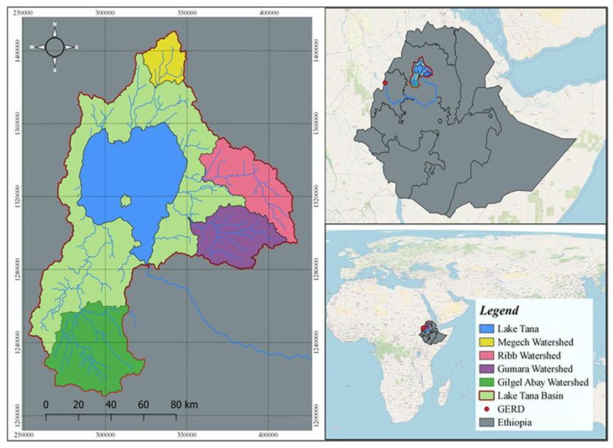
2.1. Study Area Description

The Lake Tana basin is geographically located in the Northwestern Highlands of Ethiopia, and it covers between 10.96° and 12.79° N and 36.88° and 38.26° E, and the area coverage of the basin is approximately 15,096 km², of which nearly one-fifth of the area (3063 km²) is covered with Lake Tana, the largest lake in Ethiopia (Figure 1). Even though there are other ungauged small rivers, the Lake Tana basin consists of four major gauged watersheds including Ribb, Gilgel Aba, Megech, and Gumara watersheds that are contributing more than 93% of the flow of the lake [22]. Among all major watersheds, Gilgel Abay is the largest one, which covers 1754 km², whereas Ribb, Gumara, and Megech watersheds cover 1407 km², 1272 km², and 514 km², respectively. According to [23], most of the rainfall (70–90%) of the total rainfall in the region occurs during the summer/Kiremt season from June to September. In the study area, the mean annual rainfall ranges from 1100 to 1700 mm based on data from 1971 to 2007. In Lake Tana basin and the region, temperature varies between 9 °C and 28 °C. The elevation ranges of Gilgel Abay, Gumara, Ribb, and Megech watersheds are 1885–3534 m, 1797–3585 m, 1793–4112 m, and 1864–2972 m above sea level, respectively.

According to [24], the Lake Tana basin consists of ten major soil types including eutric fluvisols, chromic luvisols, eutric leptosols, eutric cambisols, eutric regosols, eutric vertisols, haplic alisols, lithic leptosols haplic luvisols, and haplic nitisols. Because agriculture is the major economic activity of the community in the Lake Tana basin, 51.3% of the total area of the basin is covered by crop cultivation, whereas 29% and 20% of the basin has been covered by agro-pastoral area, and lake water, respectively [25].

2.2. Hydro-Meteorological Data Collection and Processing

The Meteorological station data of different periods were collected from the Ethiopian national meteorological agency. Among those, some of the stations that had data for thirty years from 1971 to 2000 were used to verify the results of the climate models. In the region, meteorological stations are not adequate in number, and even the exiting stations do not store the instruments required to measure all important climate variables for hydrological modeling. In this study, twelve stations that have better historical temperature and rainfall data were selected (

Table 1. The location, altitude and accessed climate variables of meteorological stations.

Stations	Latitude	Longitude	Altitude (Meter)	Accessed Data
				Temperature	Rainfall
Gondar	12.3	37.25	1973	1952–2009	1952–2009
Makisegnit	12.39	37.55	1912	1987–2008	1996–2008
Addis Zemen	12.12	37.77	1940	1996–2009	1997–2009
Debretabor	11.86	37.99	2612	1951–2009	1951–2009
Werota	11.92	37.69	1819	1992–2008	1969–2007
Wanzaye	11.78	37.67	1821	2000–2009	1984–2008
Bahir Dar	11.60	37.36	1800	1961–2009	1961–2009
Dangila	12.25	36.84	2125	1954–2009	1954–2009
Injibara	10.99	36.92	2568	1984–2008	1954–2008
Adet	11.27	37.49	2179	1989–2009	1989–2009
Sekela	10.98	37.21	2715	1989–2008	1988–2008
Wetet Abay	11.37	37.04	1920	1987–2008	1987–2008

).

The future climate data were projected using six Global Climate Models (GCMs) mentioned in (

Table 2. Climate models with their description, climate variables, and data used.

Climate Model	Description	Institution and Country	Climate Variables	Data Used
CanESM2	The second-generation Canadian Earth System Model	Canadian Centre for Climate Modelling and Analysis (CCCma), Canada	Tmax Tmin Precipitation	1971–2100
EC-EARTH	A European community Earth System Model	ECMWF (European Centre of Medium-Range Weather Forecast)	Tmax Tmin Precipitation	1971–2100
CNRM-CM5	Centre National de Recherches Météorologiques—Groupe d’études de l’Atmosphère Météorologique	(Centre National de Recherches Météorologiques—Groupe d’études de l’Atmosphère Météorologique) and Cerfacs (Centre Européen de Recherche et de Formation Avancée), France	Tmax Tmin Precipitation	1971–2100
HadGEM2-ES	Hadley Centre Global Environment Model version 2	Met Office Hadley Centre, UK	Tmax Tmin Precipitation	1971–2100
NORESM1-M	The Norwegian Earth System Model version 1	Norwegian Climate Centre, Norway	Tmax Tmin Precipitation	1971–2100
CSIRO-Mk3-6-0	Commonwealth Scientific and Industrial Research Organization	Commonwealth Scientific and Industrial Research Organization, Australia	Tmax Tmin Precipitation	1971–2100

Notes: T_max = Maximum Temperature, T_min = Minimum Temperature.

) under the highest emission scenario of Representative Concentration Pathway (RCP8.5) in the Coupled Model Inter-comparison Project Phase 5 (CMIP5). For this study, three important climate variables such as precipitation, minimum temperature, and maximum temperature were projected starting from the 1971 to 2100 time series data, and from which the data series from 1971 to 2000 were used for bias correction, whereas the data from 2011to 2100 were also used for evaluation of future change.

2.3. Bias Correction of Climate Models Data

The watershed-based hydrological models are mostly used to assess the potential impacts of future climate change on the components of hydrological cycles. Local topographical differences such as mountains strongly affect the simulations of temperature and rainfall by coarse-resolution climate models. Therefore, correcting the biases which may have been created in simulations of these climate variables is highly recommended. In this study, the bias of climate model outputs in the simulation of both maximum and minimum temperature was corrected by using the variance scaling approach, whereas rainfall outputs were corrected by power transformation algorism using CMhyd 2016 software [26]. Among many other methods, these two bias correction approaches were selected based on their efficiency in frequency-based statistics verified by other studies [27,28]. The historical observed data of maximum temperature, minimum temperature, and rainfall are taken between 1971 and 2000 for bias correction process.

According to [26], CMhyd software was developed to generate simulated climate data that can represent meteorological stations used in a watershed-based hydrological model setup. A transformation algorism was employed in bias correction processes for adjusting simulated climate variables so that outputs should be closer to the reality or observed data.

2.4. Geophysical Data Collection and Processing

The geophysical inputs such as soil, land use/cover, and elevation (DEM) have been used as input in SWAT model for hydrological simulation. The land use/cover of the Lake Tana basin were obtained from the Ethiopia Ministry of Water and Energy (MoWE), and the naming of each land use classes was adjusted based on the lookup table format of SWAT model. Soil data of the basin were also obtained from Food and Agriculture of United Nation Soil Map of the World with 1:5,000,000 scale [24]. The Shuttle Radar Topography Mission (SRTM) Digital Elevation Model (DEM) data were obtained from the United State Geological Survey (USGS) agency. The elevation data were used in the process of setting up of SWAT model to determine flow paths of streams and delineate the entire watersheds. Additionally, it was also used to define slopes of watersheds, which are another key element in Hydrological Response Unit (HRU) definition and analysis process combined with soil and land use data.

2.5. SWAT Model Description, Setup, and Simulation

The Soil Water Assessment Tool (SWAT) is a semi-distributed, physical-based watershed model. The model estimates the hydrological cycle components, including areal average rainfall, surface runoff, evapotranspiration, groundwater flow, and sediment yield in HRU level on a daily time scale. It is commonly aappliedto simulate both the combined and discrete impact of climate change and land use changes on both the quantity and quality of water [29].

The digital elevation data of the study area was taken for river networking and watershed delineation through the “burn-in” method. This method of a stream network theme improves hydrographic division and delineation the of boundaries of sub-watersheds. In the delineation process, the flow outlet locations where the ground-measured data are taken were selected for the four watersheds, and each watershed was delineated by the combination of many small sub-watersheds. The sub-watersheds were also further classified into the smallest spatial units named Hydrological Response Units (HRUs) by overlaying the soil, land use, and slope classifications. In the HRU definition process, all the predefined thresholds of land use, soil, and slope classes in the entire watersheds were taken into consideration. Surface runoff is generated at the HRU level and it is routed in each sub-basin level and from all sub-basins to the outlets of watersheds using the following equation (Equation (1)) [29]:

$$S{W}_t=S{W}_0+{\displaystyle \sum }_{i=1}^t{\left(R_{day}-Q_{surf}-E_a-W_{sweep}-Q_{gw}\right)}_i,$$

(1)

where SW_t is the total soil water content (mm), SW₀ is the soil water content of the day before rainfall starts (mm), t is time (days), R_day is the measure of rainfall on the day i (mm), Q_surf is the measure of surface runoff on the day i (mm), E_a is the amount of water lost by evapotranspiration on the day i (mm), W_sweep is the amount of water joining the vadose zone from the soil profile on the day i, and Q_gw is the amount of water percolated to join the groundwater on the day i (mm). The measure of surface runoff is computed using Equation (2),

$$Q_{surf}=\frac{{\left(R_{day}-I_a\right)}^2}{\left(R_{day}-I_a+S\right)},$$

(2)

where I_a is the initial abstractions (mm) and S is the retention parameter which is computed using Equation (3):

$$S=25.4\left(\frac{1000}{CN}-10\right),$$

(3)

where CN is the curve number for the day and the initial abstractions (I_a) are usually estimated as 0.2S. Therefore, by substituting, Q_surf can also be computed using (Equation (4)):

$$Q_{surf}=\frac{{\left(R_{day}-0.2S\right)}^2}{\left(R_{day}+0.8S\right)}.$$

(4)

Therefore, runoff will occur only when the amount of rainfall (R_day) is greater than the initial abstraction (I_a).

2.6. SWAT Model Calibration and Validation

In our previous study [30], the Soil and Water Assessment Tool (SWAT) has been calibrated and validated using model parameters. The calibration is performed using 1995–2002 climate data, whereas the validation of calibrated parameters has also been performed using 2003–2006 data. The overall efficiency of the model in terms of Nash Sutcliff Efficiency (NS) and Relative Volume Error (RVE) was evaluated and the maximum possible efficiency obtained from the previous study in the four watersheds (

Table 3. SWAT model efficiency in simulation of stream flow of watersheds.

Watersheds	Calibration		Validation		Default Efficiency
	NS	RVE (%)	NS	RVE (%)	NS	RVE (%)
Gilgel Abay	0.86	1.31	0.84	1.36	0.15	32.41
Gumara	0.67	1.25	0.63	1.88	0.18	36.84
Ribb	0.71	1.14	0.74	1.07	0.09	28.69
Megech	0.51	−8.84	0.54	−6.62	−0.32	−48.52

Note: Source: Reprinted/adapted with permission from [30].

).

Therefore, for this study, a new calibration process of the SWAT model was not performed; the calibrated parameters with their fitted value were simply obtained from the previous study, and the stream flow was simulated using those parameters. The calibrated parameters, with their description, range of values to iterate, fitted value, and degree of sensitivity, are presented in

Table 4. Hydrological parameters used in SWAT model.

Watershed	Parameter	Description	t-Stat	p-Value	Minimum Value	Maximum Value	Fitted Value	Rank
Gumara	R_CN2.mgt	Initial SCS CN II value	−10.14	0	0	1	0.14	1
	V_ALPHA_BF.gw	Base flow alpha-factor (days)	5.48	0	−25	25	−12	2
	V_ESCO.hru	Soil evaporation compensation factor	−3.07	0.03	0	1	0.42	3
	V_GW_DELAY.gw	Groundwater delay (days)	−2.9	0.09	0	10	7.34	4
	V_GW_REVAP.gw	Groundwater “revap” coefficient (days)	−2.23	0.11	0.02	0.2	0.19	5
Gilgel Abay	R_CN2.mgt	Initial SCS CN II value	−58	0	−0.2	0.2	−0.18	1
	V_ALPHA_BF.gw	Base flow alpha-factor (days)	10.8	0	0	1	0.12	2
	A_SOL_K.sol	Saturated hydraulic conductivity (mm/h)	6.1	0	−0.5	1	0.47	3
	V_GW_REVAP.gw	Groundwater “revap” coefficient (days)	−1.2	0.2	0.02	0.2	0.10	4
	V_GWQMN.gw	Threshold water depth in the shallow aquifer for flow (mm)	1	0.3	0	10	1.31	5
Ribb	V__ESCO.hru	Soil evaporation compensation factor	3.76	0.01	0	1	0.5	1
	R__SOL_AWC.sol	Available water capacity (mm water/mm soil)	3.55	0.01	0	1	0.9	2
	V__EPCO.hru	Plant uptake compensation factor	2.55	0.04	0	1	0.7	3
	R__CN2.mgt	Initial SCS CN II value	−1.95	0.09	−0.2	0.2	2.37	4
	V__ALPHA_BF.gw	Base flow alpha-factor (days)	1.77	0.12	0	1	0.5	5
Megech	R__CN2.mgt	Initial SCS CN II value	−10.55	0.00	−0.2	0.2	−0.02	1
	V_ALPHA_BF.gw	Base flow alpha-factor (days)	−8.27	0.00	0	1	0.76	2
	V_GW_DELAY.gw	Groundwater delay (days)	−2.70	0.01	0	10	5.37	3
	V_GWQMN.gw	Threshold water depth in the shallow aquifer for flow (mm)	2.26	0.03	0	2	0.55	4
	A_SOL_K.sol	Saturated hydraulic conductivity (mm/h)	1.90	0.06	−0.5	1	−0.17	5

.

2.7. Selection and Analysis of High Flow and Low Flow of Watersheds

In this study, the high-flow and low-flow selection and analysis are performed to evaluate the degree to which the climate change, most importantly the change in rainfall and temperature, is affecting and going to affect the extreme flow trends of watersheds in this century. The high flow as well as the low flow of watersheds were selected in the daily simulated flow output of the SWAT model for the entire study period (1971–2100).

There are different methods of low-flow selection models from the normal daily time series flow data based on the number of consecutive days which has the lowest flow of the year. The most commonly used methods are 3-day sustained mean annual low flow, 7-day sustained mean annual low flow, and 10-day sustained mean annual low flow, which are defined as the mean value of the lowest flow of the three, seven, and ten consecutive days, respectively. For this study, the 7-day sustained method is used in selecting low flow from the daily annual flow of the whole period. After the daily flow is obtained from the SWAT model, the whole 120 years of daily flow data were sorted from lowest to largest values of flow in the annual time frame, the lowest 7 days of flows in each year were selected and the mean values of each selected flows were also calculated.

Once the low flow of each year was selected, the Flow Duration Curve for the four-time period was plotted to compare changes in the three periods compared to the baseline period (1971–2000). The process of plotting FDC passes four important steps: (1) the daily annual low flow data of every period are sorted in terms of descending order; (2) the rank is assigned for each value starting from the lowest value to the highest one; (3) the probability of non-exceedance for each value is computed in terms of Weibull formula percentile (Equation (5)), and (4) the Flow Duration Curve (FDC) of the four periods are plotted using the sorted value of the four periods versus the percent of non-exceedance.

The frequency of high flows in time series data is commonly used for flood management, and safety analysis of water work constructions constructed for different purposes such as irrigation, hydropower, and other projects. For this study, the purpose of plotting Flow Duration Curve (FDC) is for evaluating the change in magnitudes of extreme flow events with respect to their frequency in the categorized time periods in the future predicted climate condition. There are two most commonly known methods of high flow selection methods in time series data, which are Annual Maximum Series (AMS) and Partial Duration Series (PDS). In AMS method, one maximum is selected from each year, whereas in Partial Duration Series (PDS), the threshold will be set and the peak values that are above that threshold will be selected as a high flow for analysis. For this study, the Annual Maximum Series (AMS) method was used for the selection of high extreme flow of the four watersheds in 120 years. Since only one highest flow is selected each year, a total of 120 peak flows are selected for analysis. Like in low-flow analysis, the Flow Duration Curve is also plotted for high flows by which the change in the high flow because of climate change is clearly shown on the curve plotted in all periods including the baseline period. The procedures to plot the Flow Duration Curve (FDC) are the same as those used in low flow except in ordering of the time series data, where, the order is descending in case of high flow. The X-axis on the plot in the high-flow duration curve is representing the exceedance probability, whereas the low-flow duration curve represents the percentile of non-exceedance probability.

$$P=\frac{M}{\left(N+1\right)}\ast 100,$$

(5)

where P is the exceedance probability of each value with in the thirty years of data; M is the rank of each value, and N, is the total number of data.

The change has also been evaluated in terms of comparison of extreme events with respect to the probability of exceedance of each event through categorizing in five ranges of the probability of exceedance in percent. These categories include Q₀–Q₂₅, Q₂₆–Q₅₀, Q₅₁–Q₇₅, and Q₇₆–Q₁₀₀, where, the mean values of extreme events in each category were also computed. Therefore, the changes in both high flow and low flow of the watersheds were evaluated by comparing the mean values of each exceedance probability in the case of high flow and non-exceedance probability in the case of low flow of the three periods with the baseline one.

3. Results and Discussion

3.1. Errors of Climate Models

The efficiency of climate models has been evaluated before and after the bias correction was performed. The default efficiency of climate models has been improved by the bias correction process. After the bias correction process result, the maximum possible error bounds of all climate models were evaluated. The errors of climate models before and after bias correction in the three climate variables are analyzed on monthly time scale. The purpose of minimizing the deviation of rainfall and both the minimum temperature and minimum temperature outputs is to minimize the bias and enhance the consistency of in simulation of stream flow of watersheds by SWAT model.

Before the biases were corrected, the default errors of climate models in the simulation of rainfall ranged from 2.11% to 6.87% including over- and under-estimations in which the lowest error was observed by CSIRO-Mk3-6-0 in January, whereas the highest error was observed by CNRM-CM5 in April (

Table 5. Errors of climate models in simulation of climate variables.

Months	Rainfall Model Error (%)
	CanESM2		EC-EARTH		CNRM-CM5		HadGEM2-ES		NORESM1-M		CSIRO-Mk3-6-0
	BBCr	ABCr	BBCr	ABCr	BBCr	ABCr	BBCr	ABCr	BBCr	ABCr	BBCr	ABCr
January	3.71	0.14	3.09	0.06	4.77	0.83	4.02	0.57	3.92	0.54	2.11	0.05
February	4.19	0.52	4.71	0.84	4.82	0.66	3.56	0.38	5.59	0.83	2.39	0.12
March	4.69	0.81	4.89	1.23	6.34	1.28	2.13	0.08	4.03	0.622	6.51	1.33
April	5.81	1.05	−4.7	−1.44	6.87	1.33	3.4	0.41	−3.09	−0.33	−4.68	−0.75
May	−5.61	−1.89	−3.89	−0.84	4.93	1.55	4.32	1.24	−4.87	−1.52	3.28	0.72
June	−5.37	−1.21	5.78	1.71	6.45	1.58	−5.93	−1.61	5.95	1.41	4.29	0.84
July	−6.09	−1.94	6.01	1.96	−5.89	−1.85	−6.49	−1.85	5.81	1.81	5.43	1.64
August	5.88	1.77	5.91	1.84	6.22	1.92	6.63	1.88	6.27	1.94	5.9	1.78
September	5.52	1.69	5.03	1.36	−4.11	−1.04	2.76	0.42	5.35	1.61	4.39	1.17
October	5.38	1.51	−3.99	−1.08	4.05	0.94	4.09	0.96	−5.05	−1.37	3.79	0.83
November	4.6	0.79	4.23	0.41	4.46	0.75	2.62	0.25	6.55	1.35	4.77	0.84
December	4.03	0.72	3.74	0.17	2.55	0.23	3.83	0.66	3.12	0.42	1.43	−0.14
Average	2.23	0.33	2.57	0.52	3.46	0.68	2.08	0.28	2.80	0.61	3.33	0.70
Model errors in maximum temperature (°C)
January	0.67	0.24	0.39	0.14	−0.61	−0.22	0.03	0.01	0.17	0.08	0.11	0.04
February	0.83	0.02	0.61	0.22	0.14	0.06	1.66	0.04	0.25	0.13	0.89	0.19
March	0.41	0.36	0.07	0.06	−0.32	−0.28	0.05	0.04	0.06	0.05	0.28	0.25
April	1.04	0.31	0.37	0.11	1.11	0.33	1.07	0.32	0.71	0.22	0.91	0.27
May	0.83	0.14	0.83	0.14	1.26	0.50	0.97	0.32	1.06	0.23	0.99	0.28
June	0.51	0.35	−0.47	−0.32	0.07	0.05	0.29	0.20	−0.09	−0.06	0.10	0.07
July	0.21	0.04	0.95	0.18	−1.04	−0.35	−0.84	−0.16	0.05	0.01	−0.58	−0.15
August	−0.75	−0.17	−1.19	−0.27	0.09	0.02	−0.35	−0.08	−0.72	−0.17	−0.53	−0.12
September	0.86	0.20	−0.30	−0.07	−0.60	−0.14	0.13	0.03	−0.09	−0.02	0.04	0.01
October	−0.48	−0.13	1.22	0.33	1.25	0.44	0.59	0.16	0.84	0.24	0.88	0.20
November	−0.16	−0.09	−0.34	−0.19	0.44	0.25	0.14	0.08	−0.11	−0.06	0.16	0.09
December	0.79	0.27	0.20	0.07	0.97	0.33	0.88	0.30	0.56	0.19	0.89	0.24
Average	0.40	0.13	0.20	0.03	0.23	0.08	0.39	0.11	0.22	0.07	0.35	0.11
Model errors in minimum temperature (°C)
January	0.18	0.07	0.42	0.11	−0.49	0.04	0.35	0.00	0.39	−0.22	0.36	−0.04
February	−0.4	−0.15	−0.90	0.03	0.92	0.12	0.06	−0.07	−0.12	0.07	1.02	0.01
March	−0.39	−0.12	0.22	−0.03	−0.02	−0.06	−0.34	−0.15	0.24	0.10	1.52	−0.03
April	0.09	0.01	0.36	0.06	0.55	0.05	0.39	−0.01	1.20	−0.14	1.60	−0.03
May	1.12	0.20	1.22	0.17	1.17	0.19	1.21	0.22	1.26	0.17	1.66	0.19
June	0.21	0.09	0.18	−0.11	−0.38	−0.19	0.44	0.02	0.11	0.00	0.47	−0.03
July	1.25	0.24	1.25	0.21	1.14	0.18	−0.60	0.21	0.57	−0.07	−0.19	0.12
August	−0.42	−0.17	−0.60	−0.22	0.43	−0.02	−0.42	0.19	−0.42	−0.15	−0.02	−0.06
September	1.15	0.20	0.04	0.07	−0.27	−0.03	0.87	0.12	0.25	−0.01	0.38	0.06
October	−0.23	−0.13	0.79	0.10	1.67	0.35	1.04	0.21	1.39	0.22	1.22	0.18
November	0.1	−0.09	−0.17	−0.14	1.21	0.06	1.05	0.21	0.18	0.02	0.58	0.03
December	1.61	0.27	0.97	0.17	0.89	0.11	0.75	0.14	1.23	0.21	1.47	0.17
Average	0.36	0.04	0.32	0.04	0.57	0.07	0.40	0.09	0.52	0.02	0.84	0.05

Notes: BBCr stands for “Before Bias Correction“, and ABCr stands for “After Bias Correction“.

). The model error of rainfall shows the negative and positive oscillation from the observed value that ranges from ±0.05% to 1.94%. When we compared the climate models, the highest inefficiency was observed by the NORESM1-M climate model in August, whereas the best-fit value was simulated by CSIRO-Mk3-6-0 in January. Seasonally, more or less all climate models were consistent reasonably with the measured rainfall, especially from November to February (Table 5). Indeed, in the region, rainfall is mostly common in the summer season and the errors of climate models are more visible in this season.

In the simulation of maximum temperature, the default model error was highest in the HadGEM2-ES climate model in February, which overestimated it by 1.66 °C (Table 5). After the errors have been corrected, most climate models projected maximum temperature with some overestimation compared to the measured data; for instance, it is overestimated in all months except July and August in the CSIRO-Mk3-6-0 climate model. From December to May, except CNRM-CM5, all the other climate models overestimated maximum temperature compared to the ground observed data. In general, the error bounds of climate models in predicting maximum temperature range from ±0.01 °C to 0.5 °C, CSIRO-Mk3-6-0 and HadGEM2-ES being more efficient in producing the data in September and January, respectively (Table 5).

Like rainfall and maximum temperature, the default efficiency of climate models in simulation of minimum temperature was evaluated and the error bounds ranged from −0.02 °C by CNRM-CM5 in March to 1.67 °C by the same model in October. After bias correction process, in the simulation of minimum temperature, almost all climate models were more efficient compared to their efficiency in the simulation of maximum temperature. The error bounds of all climate models ranged from ±0.01 °C to 0.35 °C (Table 5), in which the maximum deviation was shown by CNRM-CM5 in October.

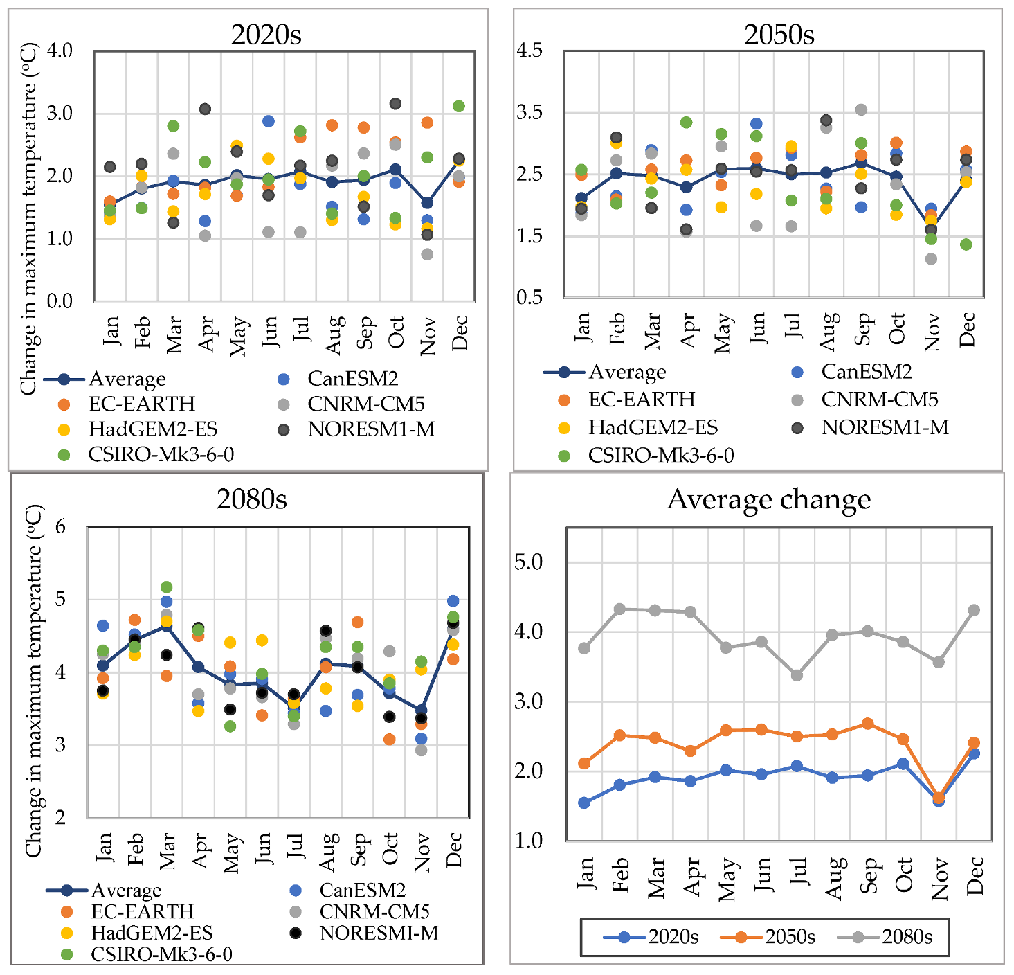
3.2. Change in Maximum Temperature

In the simulation of the hydrological process, the SWAT model uses both maximum temperature and minimum temperature to estimate evapotranspiration in the water balance computation algorism. In the highest emission of the Representative Concentration Pathway scenario (RCP8.5), the maximum temperature has shown a visible increment in the region. The highest change is expected to be observed in the 1980s period compared to the others, in which the change ranges from 2.93 °C in November by CNRM-CM5 to 5.17 °C in April by CSIRO-Mk3-6-0 in monthly time scales. Seasonally, the changes in maximum temperature in the 2020s and 2050s have also been likely to range from 0.75 °C in November by CNRM-CM5 to 3.07 °C in April by NORESM1-M, and 1.13 °C in November by CNRM-CM5 to 3.55 °C in November by CNRM-CM5, respectively. In this period, the average annual change in maximum temperature in the ensemble of six climate models is likely to be 3.9 °C. Comparatively, the highest increment in maximum temperature in the mean monthly time scale is simulated by EC-EARTH in the 2020s and 2050, and CSIRO-Mk3-6-0 in 2080s, by which it is likely to be 2.17 °C, 2.55 °C, and 5.17 °C, respectively. In an annual basis, the maximum temperature is expected to rise by 1.91 °C, 2.40 °C, and 4.04 °C in the 2020s, 2050s, and 2080s, respectively, using the ensemble mean of six climate models (Figure 2). For this study, the SWAT model uses the Hargreaves method for the computation of potential evapotranspiration in the simulation process. Therefore, as far as the method uses both maximum and minimum temperatures as input, the increment of maximum temperature has directly affected the amount of water losses by evapotranspiration in the watersheds [15,31,32].

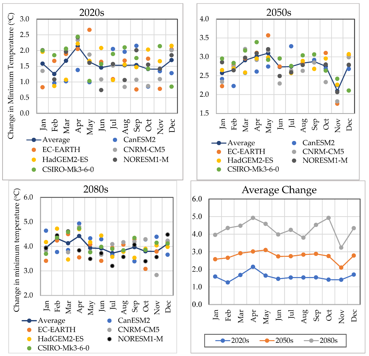
3.3. Change in Minimum Temperature

On a monthly time scale, the mean minimum temperature is showing a consistently increasing pattern in all periods, even though it is more prominent in the 2080s. The highest increment is likely to raise up to 4.75 °C as predicted by CSIRO-Mk3-6-0 in April. The overall change in minimum temperature is showing a consistently increasing pattern from the baseline to the 2020s, 2050s, and 2080s. In comparison, EC-EARTH climate model predicts the highest increment in the 2020s and 2050s, by which the change is likely to increase by 2.66 °C, and 3.57 °C, respectively. In general, in a mean annual basis, it is expected to rise by 1.57 °C, 2.75 °C, and 4.28 °C in the 2020s, 2050s, and 2080s, respectively, using the ensemble of the six climate models (Figure 3). Other similar studies have also revealed that the minimum temperature is showing an increasing pattern and affecting stream flow of catchments in the region in the coming decades of this century [21,33].

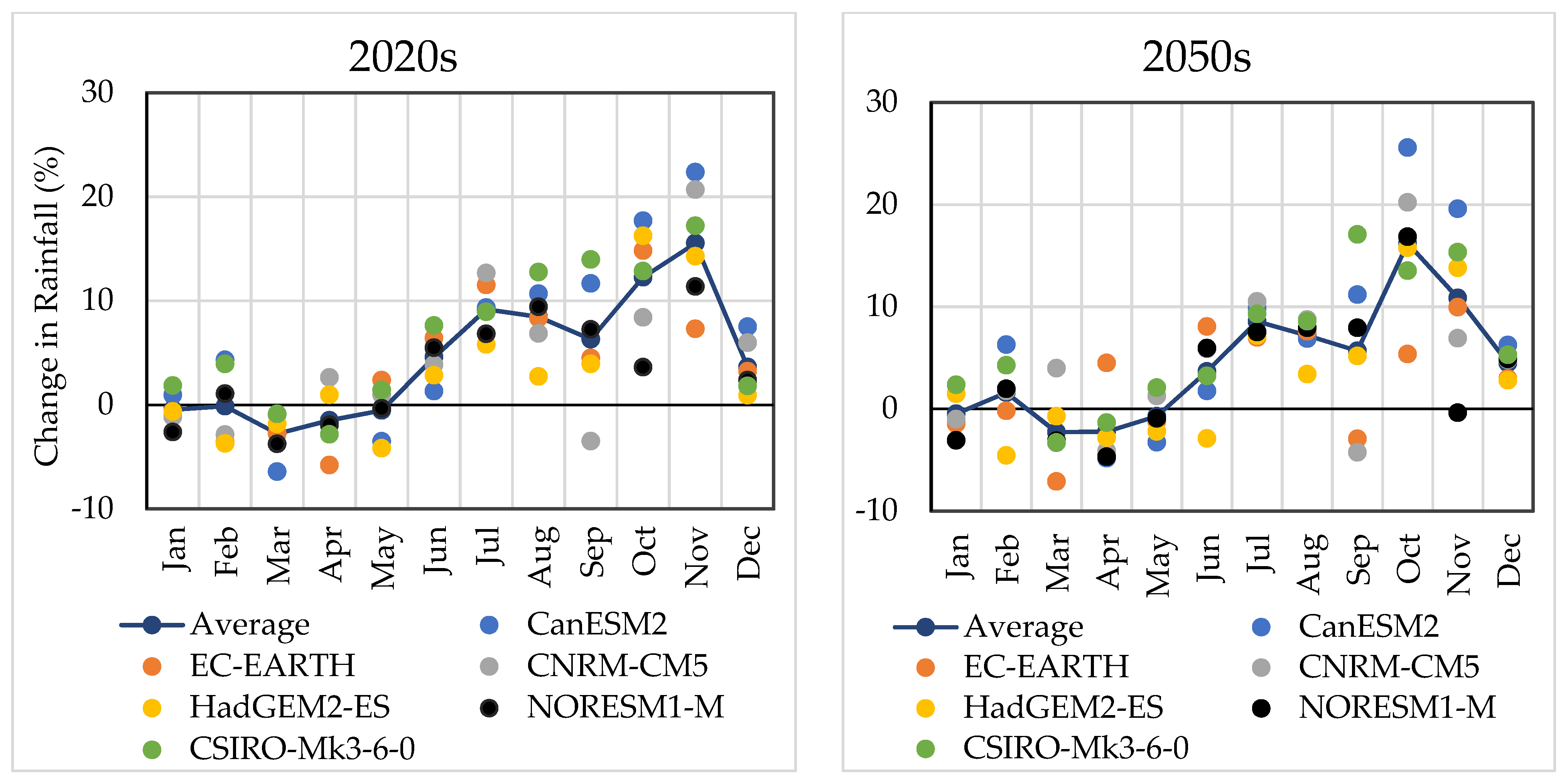
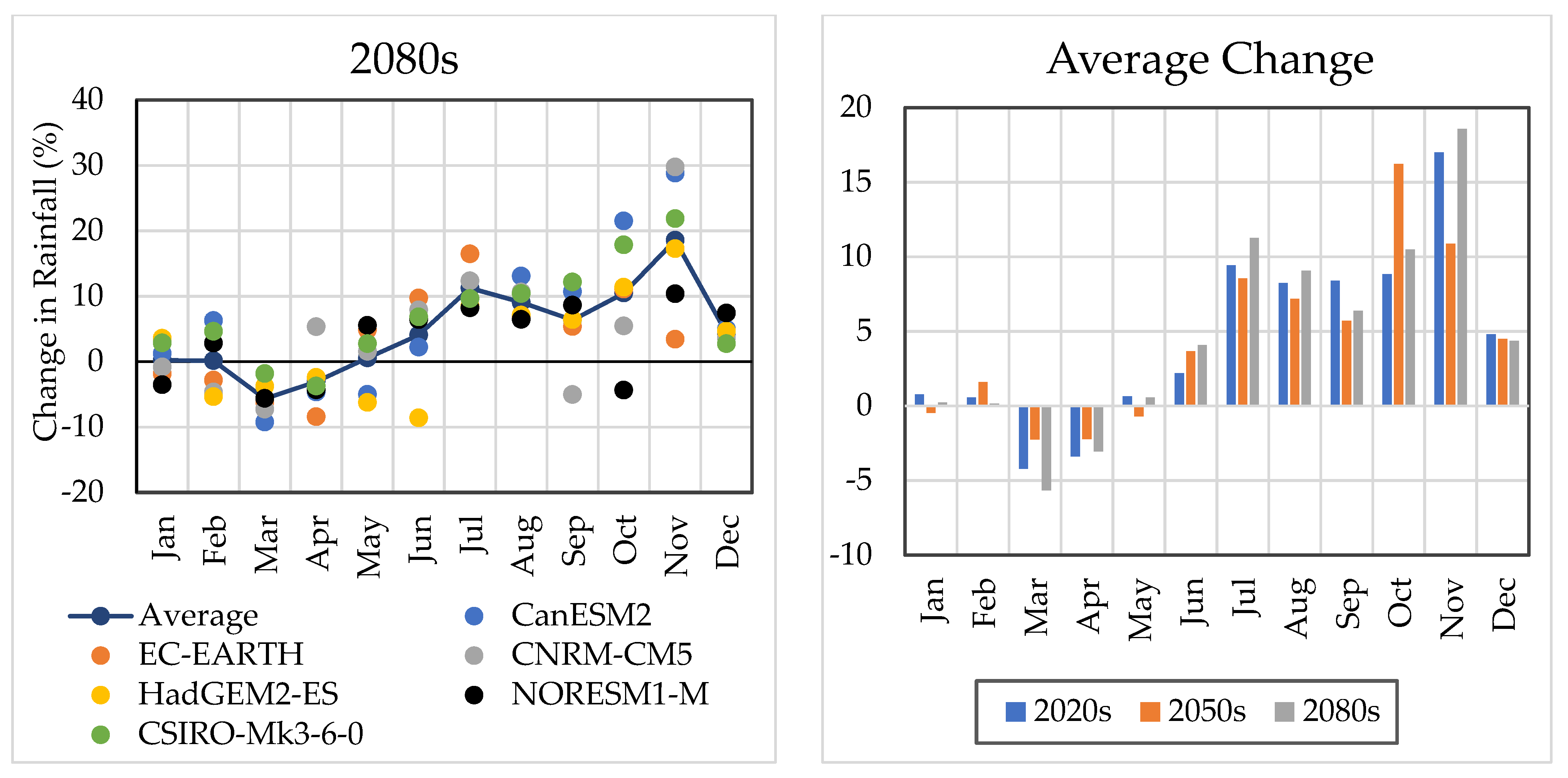
3.4. Change in Rainfall

Rainfall is expected to show both increasing and decreasing trends in the coming decades of 21st century. The change is likely to be highest in November in the 2020s and 2080s, whereas it is expected to be highest in October in the 2050s. These highest increments are expected to be 22.37% under CanESM2, 25.58% under CanESM2, and 29.75% under CNRM-CM5 in 2020s, 2050s, and 2080s, respectively. Based on most of the model outputs, rainfall is likely to decrease in the dry season, the highest decrease expected to be observed in March in all periods under the CanESM2 climate model in the 2020s and 2080s, whereas in 2050s, it is predicted by EC-EARTH climate model. The projected highest decrease in rainfall dictates the decrease of 6.42%, 7.11%, and 9.26% in the 2020s, 2050s, and 2080s, respectively. The variability of change in rainfall in average values of all climate models is also highest in the 2080s, which also dictates a 17% increase in November. The average change in all climate models showed a decrease in March and April in all periods, in which the highest decreasing change is 5.6% in the 2080s. Other previous similar studies have also indicated the inter-annual variability of change in rainfall in the region [31,33]. In general, mean annual rainfall in the basin is expected to increase by 4.43%, 4.38%, and 4.7% in the 2020s, 2050s, and 2080s, respectively (Figure 4).

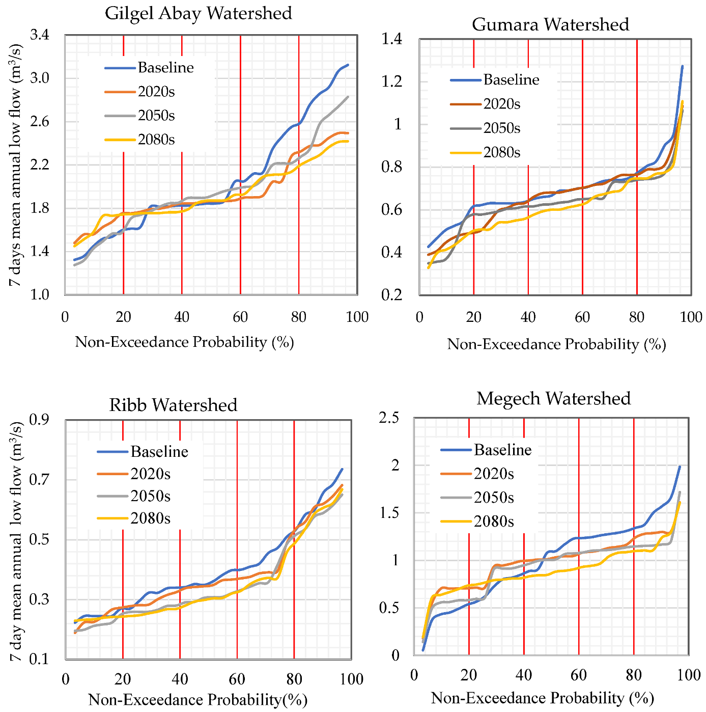
3.5. Impacts of Climate Change on Low Flow of Watersheds

The dynamics of the low flow of the four watersheds in the three periods were analyzed in terms of a simple annual average basis. The study showed that the low flow of all watersheds is likely to decrease in all periods compared to the baseline period. The low flow is predicted to decrease more prominently in the 2080s than the other periods in all watersheds. Among the watersheds, the highest decreasing trend is observed in Ribb watershed which showed a change by 5.30%, 7.57%, and 12.31% in the 2020s, 2050s, and 2080s, respectively, whereas the lowest relative decreasing trend was shown in Gilgel Abay watershed that is decreasing by 3.67%, 5.31%, and 6.8% in the 2020s, 2050s, and 2080s, respectively. In general, because of future changes in climate, the low flow is predicted to decrease by 8.39%, 8.33%, 6.21%, and 5.02% in the Ribb, Gumara, Megech, and Gilgel Abay watersheds, respectively every 30 years (

Table 6. Impacts of climate change on low flow of watersheds.

Watersheds	Average Low Flow in the Baseline Period (m3/s)	Change in Low Flow (%)			Average Change (%)
		2020s	2050s	2080s
Gilgel Abay	2.45	−3.67	−5.31	−6.8	−5.02
Gumara	0.69	−4.71	−8.51	−11.71	−8.33
Ribb	0.40	−5.30	−7.57	−12.31	−8.39
Megech	1.02	−1.45	−6.69	−10.49	−6.21

). Similar studies revealed that the low flow is reduced by the reduction of rainfall in the dry season and the shift in the rainy season [7,34,35,36] and the increment of evapotranspiration resulted by increasing in temperature [32,37]. As it is revealed by numerous studies that the low flow nature of watersheds is predominantly highly affected by the dynamics of geophysical characteristics, most importantly the change in land use/cover of the catchments plays a great role in such a way that it affects the infiltration process of water in the soil profile [38,39,40,41].

The low flow of watersheds has also been indicated in terms of Flow Duration Curves (FDC) (Figure 5) and the curves clearly showed the degree to which climate change is likely to affect the low flow of watersheds by comparing the position of curves. The low flows of the four periods which have the same non-exceedance probability have been compared through the five categories. Thus, in the Gilgel bay watershed, the magnitudes of low flows which have the non-exceedance probability in terms of percentile ranged in Q₇₆–Q₁₀₀ are showing the highest decrement change which is likely to be 15.24% every thirty years. In the Gumara watershed, the change in low flow is more prominent in Q₀–Q₂₅, which dictates that it is expected to decrease by 0.073 m³/s (13.74 %), 0.071 m³/s (13.44%), and 0.094 m³/s (17.70%) in the 2020s, 2050s, and 2080s, respectively (Table 7). The change in low flow in the Ribb watershed is showing decreasing trend in all periods and all categories of non-exceedance probability in which the highest decreasing trend is expected to be −18.45% in Q₀–Q₂₅ and 2080s. Unlike other watersheds, in Megech and Gilgel Abay watersheds, the low flows which have a non-exceedance probability range of Q₀–Q₂₅ are expected to increase in the three periods. In the Gilgel Abay watershed, these lowest flows are expected to increase by 1.64%, 11.86%, and 12.70% in the 2020s, 2050s, and 2080s, respectively, whereas in the Megech watershed, they are likely to increase by 47.06%, 21.27%, and 47.96% in 2020s, 2050s, and 2080s, respectively.

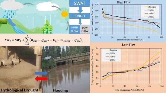
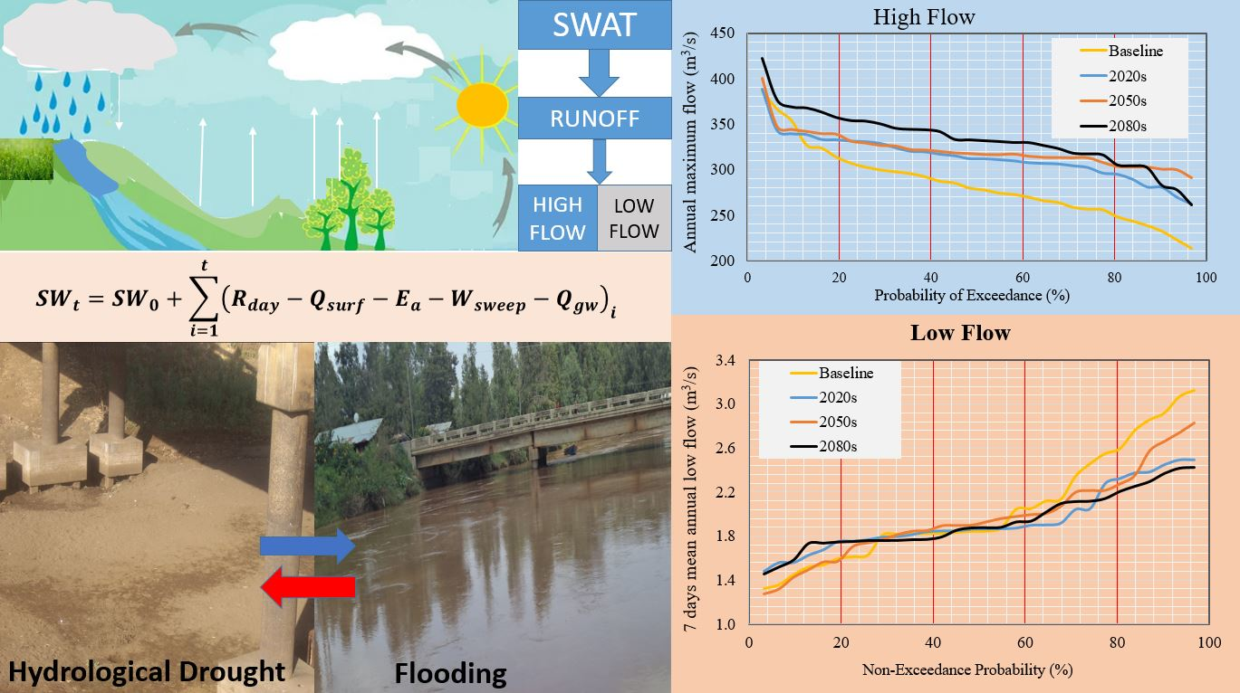
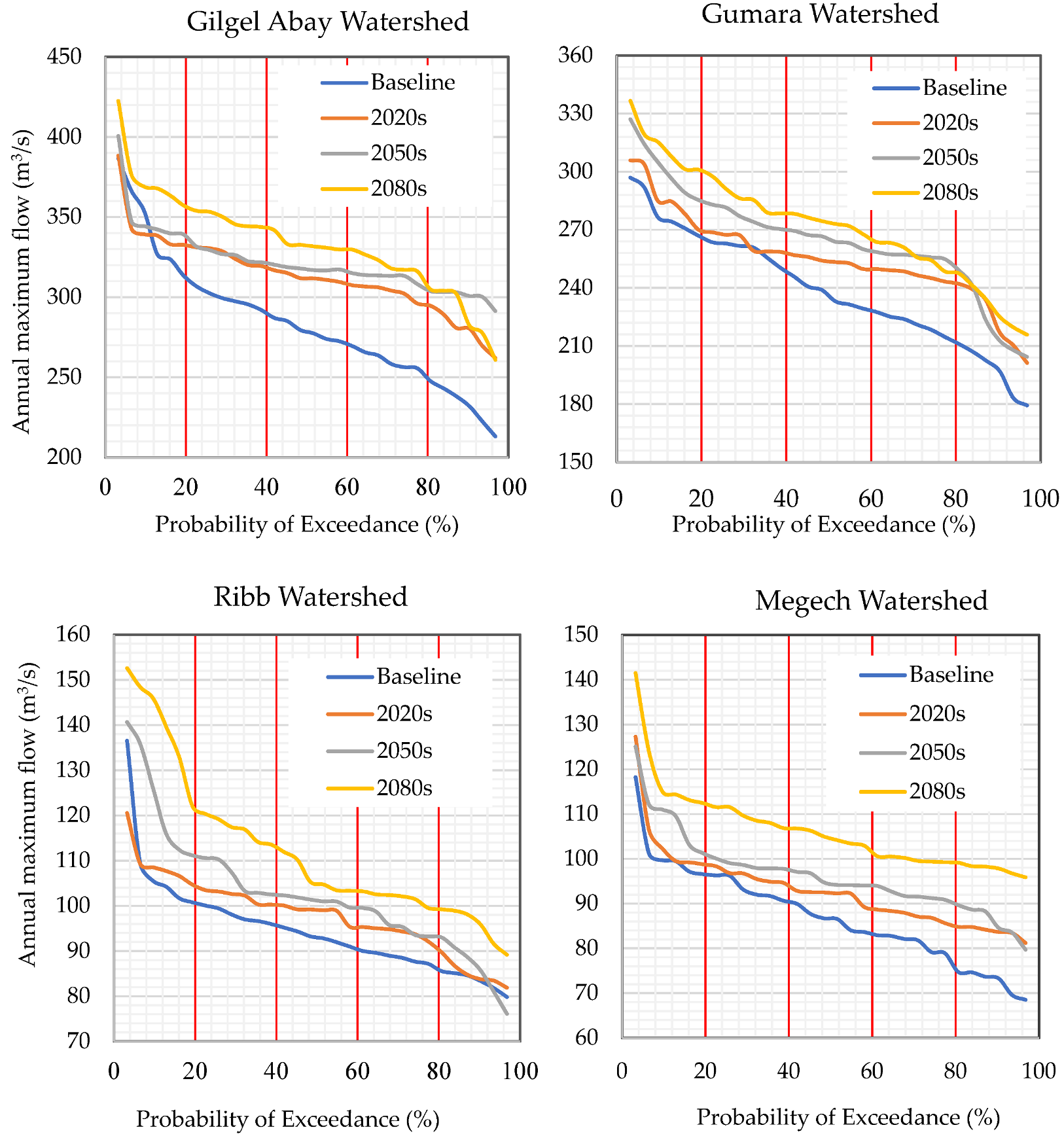
3.6. Impacts of Climate Change on High Flow of Watersheds

Annually, the change in high flow showed a consistently increasing trend in all change periods in all watersheds. Among all watersheds, the change is higher in the Gilgel Abay watershed in the 2020s and 2050s, which shows an increase of 10.56% and 13.57%, respectively, whereas in 2080s, it is higher in the Megech watershed, which is expected to increase by 22.12% in the ensemble of six climate models. Moreover, this increasing change is more prominent in the 2080s compared to the other periods in all watersheds that dictated that it is predicted to increase by 22.12%, 18.67%, 17.69%, and 14.36% in Megech, Ribb, Gilgel Abay, and Gumara watersheds, respectively. In general, the high flow is likely to increase by 13.94%, 13.16%, 10.90%, and 10.24%, and in Gilgel Abay, Megech, Gumara, and Ribb watersheds, respectively, every 30 years of the 21st century using the ensemble mean results of the six climate models (Table 8). The indication of this result that showed the change in climate affects the high flow of watersheds has also been revealed by other similar studies [42,43].

The high flow of watersheds is selected from the flow simulated by the SWAT model using the Annual Maximum Series (AMS) model for all periods in all watersheds. The selected maximum flows of all periods are plotted using Flow Duration Curve (FDC), and the result indicated that there is a great variation between all periods (Figure 6). The change in the high flow of watersheds has been evaluated by categorizing the magnitudes of flows in five classes based on their probability of exceedance (Q₀–Q₂₅, Q₂₆–Q₅₀, Q₅₁–Q₇₅, and Q₇₆–Q₁₀₀). Based on these categories, the change in high flow is more visible in Q₇₆–Q₁₀₀ in all watersheds except Ribb watershed. In this highest probability of exceedance category, the high flow is expected to increase by 55.95 m³/s (23.70%), 16.11 m³/s (21.97%), 29.89 m³/s (15.00%), and 5.76 m³/s (6.86%), and in Gilgel Abay, Megech, Gumara, and Ribb watersheds, respectively, every thirty years (Table 9). This result indicated that the change in high flow is more prominent in the minimum magnitudes. Even though it is insignificant, the high flow is decreasing by 0.15 m³/s in the lowest probability of exceedance (Q₀–Q₂₅) in the Ribb watershed by 2020s, whereas in 2050s and 2080s, it shows a significant increase, which is 12.70% and 27.81%, respectively. In all watersheds and categories of the probability of exceedance, the change in high flow is highest in the 2020s except the Gilgel Abay watershed, which is expected to show the highest increment in 2050s in Q₇₆–Q₁₀₀. Relative to all watersheds, Megech watershed is likely to experience a change of 33.53%, which is the highest increment observed in Q₇₆–Q₁₀₀ by 2080s compared to the other periods and categories of the probability of exceedance. In general, it is possible to conclude that the increment of high flow is considerably much detectable between the lowest ranges of maximum flows every thirty years in almost all watersheds.

Figure 6. Flow Duration Curve of High flows of watersheds.

Figure 6. Flow Duration Curve of High flows of watersheds.

Table 7. The mean annual low flows of watersheds in the range of probability of non-exceedance in the ensemble mean of six climate models.

Watersheds	MLF (Q0–Q25) (m3/s)				MLF (Q26–Q50) (m3/s)				MLF (Q51–Q75) (m3/s)				MLF (Q76–Q100) (m3/s)
	BlF	2020s	2050s	2080s	BlF	2020s	2050s	2080s	BlF	2020s	2050s	2080s	BlF	2020s	2050s	2080s
Gilgel Abay	1.46	1.48	1.63	1.64	1.80	1.84	1.82	1.79	2.11	2.04	1.93	1.99	2.84	2.52	2.40	2.30
Gumara	0.53	0.46	0.46	0.44	0.64	0.63	0.61	0.56	0.72	0.72	0.67	0.65	0.90	0.85	0.81	0.82
Ribb	0.25	0.24	0.24	0.24	0.33	0.32	0.30	0.27	0.41	0.38	0.36	0.34	0.62	0.59	0.59	0.57
Megech	0.41	0.61	0.50	0.61	0.84	0.95	0.91	0.81	1.22	1.08	1.08	0.95	1.53	1.31	1.24	1.22

Notes: MLF = Mean Low Flow, BlF = Baseline Flow

Table 7. The mean annual low flows of watersheds in the range of probability of non-exceedance in the ensemble mean of six climate models.

Watersheds	MLF (Q0–Q25) (m3/s)				MLF (Q26–Q50) (m3/s)				MLF (Q51–Q75) (m3/s)				MLF (Q76–Q100) (m3/s)
	BlF	2020s	2050s	2080s	BlF	2020s	2050s	2080s	BlF	2020s	2050s	2080s	BlF	2020s	2050s	2080s
Gilgel Abay	1.46	1.48	1.63	1.64	1.80	1.84	1.82	1.79	2.11	2.04	1.93	1.99	2.84	2.52	2.40	2.30
Gumara	0.53	0.46	0.46	0.44	0.64	0.63	0.61	0.56	0.72	0.72	0.67	0.65	0.90	0.85	0.81	0.82
Ribb	0.25	0.24	0.24	0.24	0.33	0.32	0.30	0.27	0.41	0.38	0.36	0.34	0.62	0.59	0.59	0.57
Megech	0.41	0.61	0.50	0.61	0.84	0.95	0.91	0.81	1.22	1.08	1.08	0.95	1.53	1.31	1.24	1.22

Notes: MLF = Mean Low Flow, BlF = Baseline Flow

Table 8. Change in high flow of watersheds because of climate change.

Watrsheds	Average High Flow in the Baseline Period (m3/s)	Change in High Flow (%)			Average Change (%)
		2020s	2050s	2080s
Gilgel Abay	283.49	10.56	13.57	17.69	13.94
Gumara	238.1	7.15	11.18	14.36	10.90
Ribb	94.53	3.56	8.50	18.67	10.24
Megech	87.10	6.72	10.63	22.12	13.16

Table 8. Change in high flow of watersheds because of climate change.

Watrsheds	Average High Flow in the Baseline Period (m3/s)	Change in High Flow (%)			Average Change (%)
		2020s	2050s	2080s
Gilgel Abay	283.49	10.56	13.57	17.69	13.94
Gumara	238.1	7.15	11.18	14.36	10.90
Ribb	94.53	3.56	8.50	18.67	10.24
Megech	87.10	6.72	10.63	22.12	13.16

Table 9. The mean annual maximum flows of watersheds in the range of probability of exceedance in the ensemble mean of six climate models.

Watersheds	MHF (Q0–Q25) (m3/s)				MHF (Q26–Q50) (m3/s)				MHF (Q51–Q75) (m3/s)				MHF (Q76–Q100) (m3/s)
	BlF	2020s	2050s	2080s	BlF	2020s	2050s	2080s	BlF	2020s	2050s	2080s	BlF	2020s	2050s	2080s
Gilgel Abay	345.09	345.77	352.31	376.11	293.90	321.93	323.92	344.27	267.13	307.30	314.98	325.81	236.02	281.84	301.49	292.57
Gumara	279.55	287.91	302.90	313.59	253.31	260.73	273.38	282.95	226.19	249.31	259.01	263.78	199.23	226.65	227.60	233.10
Ribb	109.69	109.54	123.62	140.19	96.65	101.17	104.70	114.31	90.06	95.81	98.06	102.90	83.92	86.06	86.92	96.05
Megech	102.05	105.59	110.36	120.08	91.60	94.98	97.78	108.25	82.88	89.08	92.94	101.34	73.33	83.95	86.46	97.92

Notes: MHF = Mean High Flow, BlF = Baseline Flow.

Table 9. The mean annual maximum flows of watersheds in the range of probability of exceedance in the ensemble mean of six climate models.

Watersheds	MHF (Q0–Q25) (m3/s)				MHF (Q26–Q50) (m3/s)				MHF (Q51–Q75) (m3/s)				MHF (Q76–Q100) (m3/s)
	BlF	2020s	2050s	2080s	BlF	2020s	2050s	2080s	BlF	2020s	2050s	2080s	BlF	2020s	2050s	2080s
Gilgel Abay	345.09	345.77	352.31	376.11	293.90	321.93	323.92	344.27	267.13	307.30	314.98	325.81	236.02	281.84	301.49	292.57
Gumara	279.55	287.91	302.90	313.59	253.31	260.73	273.38	282.95	226.19	249.31	259.01	263.78	199.23	226.65	227.60	233.10
Ribb	109.69	109.54	123.62	140.19	96.65	101.17	104.70	114.31	90.06	95.81	98.06	102.90	83.92	86.06	86.92	96.05
Megech	102.05	105.59	110.36	120.08	91.60	94.98	97.78	108.25	82.88	89.08	92.94	101.34	73.33	83.95	86.46	97.92

Notes: MHF = Mean High Flow, BlF = Baseline Flow.

4. Conclusions

The study revealed that future extreme flow events of the headwater catchments in the upper Blue Nile basin are expected to be significantly affected by climate change. Both the maximum temperature and minimum temperature were prominently increased in the 2080s in monthly and annual time scales, and consequently, the loss of water by evaporation from the soil and evapotranspiration from plants is expected to increase in the watersheds. Inter-annual variability of change in rainfall showed increasing and decreasing patterns on monthly time scales, whereas the variability of changes in the three periods is not significant on the annual time scale. On the monthly time scale, the maximum change in rainfall is expected to rise up to 28.79% in the 2050s as predicted by the CanESM2 climate model.

The high flow is likely to increase and even probably be changed to flooding in some areas of watersheds for the coming decades of this century. The dry season flow/low flow which contains the environmental flow of catchments is predicted to decrease in all periods because of decreasing rainfall and increasing temperature in the dry seasons in the region. Thus, concerned bodies working on different water projects and river basin management projects should consider these expected flooding and hydrological droughts of watersheds.

Besides the climate factors, the changes in land use/cover in the watersheds also considerably impact stream flow; therefore, researchers of this study suggest that the combined impacts of land use/cover change on the stream flow focusing on extreme flow nature of watersheds in the basin should be investigated using the worst climate change scenario and numerous climate models.

References

1. IPCC. IPCC, 2001: Climate Change 2001: The Scientific Basis. Contribution of Working Group 1 to the Third Assessment Report of the Intergovernmental Panel on Climate Change; Houghton, J., Ding, Y., Griggs, D., Noguer, M., van der Linden, P., Dai, X., Mas, K., Eds.; Wiley Online Library: Hoboken, NJ, USA, 2002. [Google Scholar]
2. Oreskes, N. The scientific consensus on climate change. Science 2004, 306, 1686. [Google Scholar] [CrossRef] [PubMed] [Green Version]
3. Adedeji, O. Global climate change. J. Geosci. Environ. Prot. 2014, 2, 114. [Google Scholar] [CrossRef]
4. IPCC. 2014: Climate Change 2014: Synthesis Report. Contribution of Working Groups I, II and III to the Fifth Assessment Report of the Intergovernmental Panel on Climate Change; Core Writing Team, Pachauri, R.K., Meyer, L.A., Eds.; IPCC: Geneva, Switzerland, 2014; p. 151. [Google Scholar]
5. IPCC. 2007: Climate Change 2007: The Physical Science Basis. Contribution of Working Group I to the Fourth Assessment Report of the Intergovernmental Panel on Climate Change; Solomon, S., Qin, D., Manning, M., Chen, Z., Marquis, M., Averyt, K.B., Tignor, M., Miller, H.L., Eds.; Cambridge University Press: Cambridge, UK; New York, NY, USA, 2007; 996p. [Google Scholar]
6. IPCC. 2012: Managing the Risks of Extreme Events and Disasters to Advance Climate Change Adaptation. A Special Report of Working Groups I and II of the Intergovernmental Panel on Climate Change; Field, C.B., Barros, V., Stocker, T.F., Qin, D., Dokken, D.J., Ebi, K.L., Mastrandrea, M.D., Mach, K.J., Plattner, G.-K., Allen, S.K., et al., Eds.; Cambridge University Press: Cambridge, UK; New York, NY, USA, 2012; 582p. [Google Scholar]
7. Trenberth, K.E. Conceptual framework for changes of extremes of the hydrological cycle with climate change. In Weather and Climate Extremes; Springer: Berlin/Heidelberg, Germany, 1999; pp. 327–339. [Google Scholar]
8. Trenberth, K.E.; Fasullo, J.T. Climate extremes and climate change: The Russian heat wave and other climate extremes of 2010. J. Geophys. Res. Atmos. 2012, 117, 17103. [Google Scholar] [CrossRef]
9. Karl, T.R.; Knight, R.W. Secular trends of precipitation amount, frequency, and intensity in the United States. Bull. Am. Meteorol. Soc. 1998, 79, 231–242. [Google Scholar] [CrossRef]
10. Huntington, T.G. Evidence for intensification of the global water cycle: Review and synthesis. J. Hydrol. 2006, 319, 83–95. [Google Scholar] [CrossRef]
11. Held, I.M.; Soden, B.J. Robust responses of the hydrological cycle to global warming. J. Clim. 2006, 19, 5686–5699. [Google Scholar] [CrossRef]
12. Sheffield, J.; Wood, E.F.; Roderick, M.L. Little change in global drought over the past 60 years. Nature 2012, 491, 435–438. [Google Scholar] [CrossRef]
13. Gebremicael, T.G.; Mohamed, Y.A.; Zaag, P.V.; Hagos, E.Y. Temporal and spatial changes of rainfall and streamflow in the Upper Tekezē-Atbara river basin, Ethiopia. Hydrol. Earth Syst. Sci. 2017, 21, 2127–2142. [Google Scholar] [CrossRef] [Green Version]
14. Tesemma, Z.K.; Mohamed, Y.A.; Steenhuis, T.S. Trends in rainfall and runoff in the Blue Nile Basin: 1964–2003. Hydrol. Process. 2010, 24, 3747–3758. [Google Scholar] [CrossRef] [Green Version]
15. Gizaw, M.S.; Biftu, G.F.; Gan, T.Y.; Moges, S.A.; Koivusalo, H. Potential impact of climate change on streamflow of major Ethiopian rivers. Clim. Chang. 2017, 143, 371–383. [Google Scholar] [CrossRef]
16. Bekele, W.T.; Haile, A.T.; Rientjes, T. Impact of climate change on the streamflow of the Arjo-Didessa catchment under RCP scenarios. J. Water Clim. Chang. 2021, 12, 2325–2337. [Google Scholar] [CrossRef]
17. Gurara, M.A.; Jilo, N.B.; Tolche, A.D. Modelling climate change impact on the streamflow in the Upper Wabe Bridge watershed in Wabe Shebele River Basin, Ethiopia. Int. J. River Basin Manag. 2021, 1–13. [Google Scholar] [CrossRef]
18. Worqlul, A.W.; Dile, Y.T.; Ayana, E.K.; Jeong, J.; Adem, A.A.; Gerik, T. Impact of climate change on streamflow hydrology in headwater catchments of the Upper Blue Nile Basin, Ethiopia. Water 2018, 10, 120. [Google Scholar] [CrossRef] [Green Version]
19. Roth, V.; Lemann, T.; Zeleke, G.; Subhatu, A.T.; Nigussie, T.K.; Hurni, H. Effects of climate change on water resources in the upper Blue Nile Basin of Ethiopia. Heliyon 2018, 4, e00771. [Google Scholar] [CrossRef] [PubMed] [Green Version]
20. Mengistu, D.; Bewket, W.; Dosio, A.; Panitz, H.-J. Climate change impacts on water resources in the Upper Blue Nile (Abay) River Basin, Ethiopia. J. Hydrol. 2021, 592, 125614. [Google Scholar] [CrossRef]
21. Adem, A.A.; Seifu, A.T.; Essayas, K.A.; Abeyou, W.W.; Tewodros, T.A.; Shimelis, B.D.; Assefa, M.M. Climate change impact on stream flow in the upper Gilgel Abay Catchment, Blue Nile Basin, Ethiopia. In Landscape Dynamics, Soils and Hydrological Processes in Varied Climates; Springer: Berlin/Heidelberg, Germany, 2016; pp. 645–673. Available online: https://link.springer.com/chapter/10.1007/978-3-319-18787-7_29 (accessed on 15 January 2015).
22. Setegn, S.G. Modelling Hydrological and Hydrodynamic Processes in Lake Tana Basin, Ethiopia; KTH: Stockholm, Sweden, 2010. [Google Scholar]
23. Conway, D.; Schipper, E.L.F. Adaptation to climate change in Africa: Challenges and opportunities identified from Ethiopia. Glob. Environ. Chang. 2011, 21, 227–237. [Google Scholar] [CrossRef]
24. FAO; UNESCO. FAO-UNESCO soil map of the world, 1:5,000,000. Africa. Fao Soil Bull. 1977, VI, 346. [Google Scholar]
25. Setegn, S.G.; Srinivasan, R.; Dargahi, B. Hydrological modelling in the Lake Tana Basin, Ethiopia using SWAT model. Open Hydrol. J. 2008, 2, 49–62. Available online: https://benthamopen.com/contents/pdf/TOHYDJ/TOHYDJ-2-49.pdf (accessed on 27 November 2022). [CrossRef] [Green Version]
26. Rathjens, H.; Bieger, K.; Srinivasan, R.; Arnold, J.G. CMhyd User Manual Documentation for Preparing Simulated Climate Change Data for Hydrologic Impact Studies; Online Resources; 2016; 16p, Available online: https://swat.tamu.edu/media/115265/bias_cor_man.pdf (accessed on 6 January 2023).
27. Fang, G.H.; Yang, J.; Chen, Y.N.; Zammit, C. Comparing bias correction methods in downscaling meteorological variables for a hydrologic impact study in an arid area in China. Hydrol. Earth Syst. Sci. 2015, 19, 2547–2559. [Google Scholar] [CrossRef] [Green Version]
28. Teutschbein, C.; Seibert, J. Bias correction of regional climate model simulations for hydrological climate-change impact studies: Review and evaluation of different methods. J. Hydrol. 2012, 456, 12–29. [Google Scholar] [CrossRef]
29. Neitsch, S.L.; Arnold, J.G.; Kiniry, J.R.; Srinivasan, R.; Williams, J.R. Soil and Water Assessment Tool User’s Manual; TWRI Report TR-192; Texas Water Resources Institute: College Station, TX, USA, 2002; p. 412. Available online: http://swat.tamu.edu/media/1294/swatuserman.pdf (accessed on 6 January 2023).
30. Chakilu, G.G.; Sándor, S.; Zoltán, T.; Phinzi, K. Climate change and the response of streamflow of watersheds under the high emission scenario in Lake Tana sub-basin, upper Blue Nile basin, Ethiopia. J. Hydrol. Reg. Stud. 2022, 42, 101175. [Google Scholar] [CrossRef]
31. Haile, A.T.; Akawka, A.L.; Berhanu, B.; Rientjes, T. Changes in water availability in the Upper Blue Nile basin under the representative concentration pathways scenario. Hydrol. Sci. J. 2017, 62, 2139–2149. [Google Scholar] [CrossRef] [Green Version]
32. Abtew, W.; Melesse, A. Climate change and evapotranspiration. In Evaporation and Evapotranspiration; Springer: Berlin/Heidelberg, Germany, 2013; pp. 197–202. [Google Scholar]
33. Chakilu, G.G.; Sándor, S.; Zoltán, T. Change in stream flow of gumara watershed, upper blue nile basin, ethiopia under representative concentration pathway climate change scenarios. Water 2020, 12, 3046. [Google Scholar] [CrossRef]
34. Kundzewicz, Z.W.; Krysanova, V.; Benestad, R.E.; Hov, Ø.; Piniewski, M.; Otto, I.M. Uncertainty in climate change impacts on water resources. Environ. Sci. Policy 2018, 79, 1–8. [Google Scholar] [CrossRef]
35. Moon, J.; Lee, W.K.; Song, C.; Lee, S.G.; Heo, S.B.; Shvidenko, A.; Kraxner, F.; Lamchin, M.; Lee, E.J.; Zhu, Y.; et al. An introduction to mid-latitude ecotone: Sustainability and environmental challenges. Sibirskij Lesnoj Zurnal (Sib. J. For. Sci.) 2017, 53, 41–53. [Google Scholar] [CrossRef]
36. De Girolamo, A.M.; Barca, E.; Leone, M.; Porto, A.L. Impact of long-term climate change on flow regime in a Mediterranean basin. J. Hydrol. Reg. Stud. 2022, 41, 101061. [Google Scholar] [CrossRef]
37. Parey, S.; Gailhard, J. Extreme Low Flow Estimation under Climate Change. Atmosphere 2022, 13, 164. [Google Scholar] [CrossRef]
38. Chakilu, G.G.; Moges, M.A. Assessing the Land Use/Cover Dynamics and its Impact on the Low Flow of Gumara Watershed, Upper Blue Nile Basin, Ethiopia. Hydrol. Curr. Res. 2017, 8, 1–6. [Google Scholar] [CrossRef] [Green Version]
39. Gebrehiwot, S.G.; Taye, A.; Bishop, K. Forest cover and stream flow in a headwater of the Blue Nile: Complementing observational data analysis with community perception. Ambio 2010, 39, 284–294. [Google Scholar] [CrossRef] [Green Version]
40. Mekonnen, D.F.; Duan, Z.; Rientjes, T.; Disse, M. Analysis of combined and isolated effects of land-use and land-cover changes and climate change on the upper Blue Nile River basin’s streamflow. Hydrol. Earth Syst. Sci. 2018, 22, 6187–6207. [Google Scholar] [CrossRef] [Green Version]
41. Shao, G.; Guan, Y.; Zhang, D.; Yu, B.; Zhu, J. The impacts of climate variability and land use change on streamflow in the Hailiutu river basin. Water 2018, 10, 814. [Google Scholar] [CrossRef]
42. Tian, Y.; Xu, Y.P.; Zhang, X.J. Assessment of Climate Change Impacts on River High Flows through Comparative Use of GR4J, HBV and Xinanjiang Models. Water Resour. Manag. 2013, 27, 2871–2888. [Google Scholar] [CrossRef]
43. Goulden, M.; Conway, D.; Persechino, A. Adaptation to climate change in international river basins in Africa: A review. Hydrol. Sci. J. 2009, 54, 805–828. [Google Scholar] [CrossRef]
Figure 1. Geographical location of Lake Tana basin.
Water 15 00358 g001
Figure 2. Change in maximum temperature in 2020s, 2050s, and 2080s including the average change in all climate models.
Water 15 00358 g002
Figure 3. Change in minimum temperature in 2020s, 2050s, and 2080s, including the average change in all climate models.
Water 15 00358 g003
Figure 4. Rainfall change in 2020s, 2050s, and 2080s, including the average change in all climate models.
Water 15 00358 g004aWater 15 00358 g004b
Figure 5. Flow Duration Curve of low flows of watersheds.
Water 15 00358 g005