
Investigation on Water Levels for Cascaded Hydropower Reservoirs to Drawdown at the End of Dry Seasons
by
 , ,
, ,
Shuangquan Liu
1,
Xuhan Luo
2,
Hao Zheng
2,
Congtong Zhang
1,
Youxiang Wang
1,
Kai Chen
1 and
Jinwen Wang
3,4,* 1
Yunnan Power Grid Co., Ltd., 73# Tuodong Road, Kunming 650041, China
2
School of Civil and Hydraulic Engineering, Huazhong University of Science and Technology, 1037 Luoyu Road, Wuhan 430074, China
3
Institute of Water Resources and Hydropower, Huazhong University of Science and Technology, 1037 Luoyu Road, Wuhan 430074, China
4
Hubei Key Laboratory of Digital River Basin Science and Technology, Huazhong University of Science and Technology, 1037 Luoyu Road, Wuhan 430074, China
*
Author to whom correspondence should be addressed.
Water 2023, 15(2), 362; https://doi.org/10.3390/w15020362
Submission received: 1 December 2022
/
Revised: 6 January 2023
/
Accepted: 9 January 2023
/
Published: 16 January 2023
(This article belongs to the Section Hydrology)
Abstract
:Operators often have a dilemma in deciding what water levels the over-year hydropower reservoirs should drawdown at the end of dry seasons, either too high to achieve a large firm hydropower output during the dry seasons in the current year and minor spillage in coming flood seasons, or too low to refill to the full storage capacity at the end of the flood seasons and a greater firm hydropower output in the coming year. This work formulates a third-monthly (in an interval of about ten days) hydropower scheduling model, which is linearized by linearly concaving the nonlinear functions and presents a rolling strategy to simulate many years of reservoir operations to investigate how the water level at the end of dry seasons will impact the performances, including the energy production, firm hydropower output, full-refilling rate, etc. Applied to 11 cascaded hydropower reservoirs in a river in southwest China, the simulation reveals that targeting a drawdown water level between 1185–1214 m for one of its major over-year reservoirs and 774–791 m for another is the most favorable option for generating more hydropower and yielding larger firm hydropower output.
1. Introduction
As acknowledged in work by Algarvio [1], hydroelectric, wind, and solar power plants are the most competitive renewable energy suppliers, and along with nuclear and hydrogen energies [2], are the primary sources of new energy that will dominate carbon neutrality in the future. In the context of the commitment to achieving carbon peaking and neutrality, hydropower is and will continue to play an essential role in the energy structure worldwide, especially in countries or regions rich in hydropower resources. For instance, in China’s Sichuan Province, where river hydropower is the predominant renewable energy source, Bamisile et al. [3] predicted that the carbon emission will reduce by 13.26%, 14.77%, and 15.3% between 2030 and 2050 for dry, regular, and wet year scenarios, respectively.
As one of the primary renewable energy sources, hydropower can be generated on a large scale but will soon have its potential exploited to a considerable extent. Hydropower has the world’s largest share of renewable energy sources, supplying more than 16.6% of total global electricity to over 160 countries worldwide [4]. Brazil, for instance, has significant hydroelectric potential, totaling 101,269 MW, corresponding to 60.9% of the energy matrix. The 218 hydropower plants are responsible for 60.5% of the total installed capacity in the country, adding up to 95,620 MW [5]. Hydropower is also an integral part of Europe’s energy sector, contributing 41.7% of the total electricity generation in the EU. Indeed, the proportion of national electricity generation in different European countries varies greatly from almost 100.0% (e.g., 98.3% in Norway) to small numbers (e.g., 11.7% in the United Kingdom) [6]. In China, abundant hydropower resources have provided unprecedented advantages and opportunities for rapid hydropower development over the last five decades [7]. However, as in large parts of Europe, the hydropower potential will soon be exploited practically close to its limit [6]. Aimed at economic growth and poverty alleviation, the world has experienced a boom in plans for hydropower plants over the last two decades, which, however, have not resulted in a global mass construction of hydropower plants due to factors such as the administrative complexity, over-estimations of exploitable capacity, an ugly sociopolitical and socioeconomic situation, and so on [8]. Additionally, global warming complicates the role of hydropower in the energy structure. As shown in a hydrological and techno-economic model used in work by Meng et al. [9], global warming will positively impact hydropower production in a tropical island (Sumatra). Still, the ratio of hydropower production to power demand under 1.5 °C of global warming is 40% higher than that under 2 °C of global warming, suggesting that a more unfavorable global warming will incur a more significant gap for the energy supply to meet the demand. Apparently, how to manage the hydropower projects under operation to produce more energy and provide flexible service will become a more crucial and active academic and engineering challenge in the future.
Generating more hydropower energy contributes to more economic benefits and less CO2 emission from the power systems. It can be targeted by keeping the forebay water level as high as possible to improve the generation efficiency and properly regulating the storage to reduce spillages. In California, for instance, single-purpose reservoirs are predominantly located at high elevations to take advantage of higher water heads to generate more hydropower [10]. Additionally, as demonstrated by Lu et al. [11] with case studies, a joint operation of two large upstream reservoirs could increase the electricity production of the mainstream run-off hydropower plants at the lower reaches by regulating the upstream reservoirs to reduce spillages from the downstream reservoirs. Additionally, compared with conventional coal power plants, hydropower prevents the emission of about 3 GT CO2 per year, representing about 9% of global annual CO2 emissions [12].
The hydropower systems, especially when having large reservoirs with over-year storage capacity, are expected to output powers that are consistent over months and flexible over hours to ensure the security and stability of the power systems. As targeted in work by Oven-Thompson et al. [13], the consistency of a hydropower system in power supply has long been indicated by using the firm monthly hydropower production, which is guaranteed in each month and is particularly important in dry seasons when reservoirs must draw down their water levels to increase generating discharges. Naturally, like huge batteries by refilling or emptying the water to recharge or discharge power [14], hydropower reservoirs with large active storage capacities are very flexible in peak-shaving and providing other ancillary services in power systems, which is under more significant pressure to ensure the operational security, especially with much more intermittent solar and wind powers to be integrated in future. Hirth [15], for instance, indicated that hydropower mitigated the value drop by a third when moving from 0% to 30% wind penetration, impressively with 1 MWh of wind energy worth 18% more in Sweden than in Germany. However, the flexibility of hydropower in dry seasons can only be ensured with enough firm monthly hydropower production.
Accurate prediction of monthly runoffs in the coming months is still a worldwide difficulty in hydrological engineering. The randomness of inflows imposes significant challenges in scheduling monthly hydropower generations to achieve goals, such as maximizing the firm power output and the hydropower production in total, which were often pursued by targeting certain water levels in critical months during a year, such as the year-end water level that was often investigated for over-year reservoirs [16]. The year-end water level, for instance, was approximated as a function of the inflow frequency based on the least square error principle by Jiang et al. [17], who extracted the operation rule from a sample of results derived by simulating the operation with a hydropower scheduling model to maximize energy production over 63 years of historical inflows. Liu et al. [18] treated the year-end water level as a function of the year-start water level and the inflow during the year, determined by statistic regression on a sample of results also derived with a deterministic optimization to maximize hydropower production. Zhang et al. [19] used a data mining technique of decision trees to identify an operational rule, which determined the year-end water level based on the inflow frequency, by exploiting an extensive database obtained with an operating model. All these previous works determined the year-end water level by using the inflow during the coming year, which, unfortunately, often cannot be predicted at an applicable precision. They focused on maximizing hydropower production but not the firm monthly hydropower output, and the optimization was not simulated over successive years when historical inflows were available.
This work attempts to address the dilemma that hydropower reservoir operators have in deciding on what forebay water levels should be targeted or drawn down at the end of dry seasons (referred to simply as the drawdown level) to nicely balance the firm monthly output with the total energy production, as well as the benefits in the current year with the following year. The drawdown levels can be either too high to allow more significant releases during the dry seasons to give a larger firm hydropower output in the current year and less spillage in the coming flood seasons, or too low to utilize higher water heads to generate more energy during the flooding seasons and to prepare a full storage capacity at the end of flood seasons for a greater firm hydropower output in the coming year.
The stochastic monthly inflows can be explicitly formulated into a stochastic optimization model [20], which derives an operational rule that can be simulated over many years to assess the impact of the drawdown level. Another option is to adopt a deterministic optimization strategy, of which De Souza Zambelli et al. [21] demonstrated the advantages in long-term hydrothermal scheduling of large-scale power systems. The stochastic and deterministic schemes are more convenient or applicable than another when applied in specific engineering scenarios, with the deterministic modeling more often applied to preliminary evaluation [22]. Zambelli et al. [23] demonstrated that an operation strategy based on deterministic modeling, when appropriately applied, can achieve similar performance to what is yielded with a stochastic approach. However, deterministic optimization also has dimensional difficulty as applied over a long scheduling horizon involving many years of historical monthly inflows. The solution efficiency is affected by the ways to model the hydropower output, which is a nonlinear function of the forebay water level and outflow of a reservoir. As shown by Kang et al. [24], the nonlinear hydropower output can be linearized with Special Ordered Sets (SOS) methods, introducing many binary variables that will likely make the solution procedure volatile.
This work will make contributions by (1) presenting a scroll optimization strategy to decouple a long planning horizon into much shorter scheduling horizons to alleviate the dimensional difficulty, assuming the boundary conditions at the end of a scheduling horizon will have negligible impacts on the results long enough before the end of the scheduling horizon; (2) experimenting a three-triangle-based method [25] to linearly concave the nonlinear hydropower output without introducing any integer variables, expected to improve the solution efficiency significantly; and (3) including the firm hydropower outputs, which, along with the commonly used total energy production, will be targeted in assessing optional drawdown water levels at the end of dry seasons.
2. Problem Formulation
The model aims to minimize the hydropower curtailment/spillage from reservoirs sequentially, the deficiency to contracted third-monthly electricity, and the deviations from the storages targeted at the end of the scheduling horizon, as well as to maximize the firm hydropower output and the total hydropower production, mathematically expressed as
Subject to:
(1) Water balance for a reservoir,
(2) Bounds on the storage of a reservoir,
(3) Bounds on release,
(4) Generating capacity,
(5) Contracted electricity to be met with,
(6) Firm hydropower output,
(7) Storage to be evaluated at the end of May, which is taken as the last month in dry seasons,
(8) Hydropower output,
where = hydropower curtailment of hydro-plant i in time-step t; and = negative and positive deviations, respectively from the contracted electricity of hydro-plant i in time-step t; = firm hydropower output of hydro-plant i; ,= deviations reservoir i under and over the storage target at the end of scheduling horizon, respectively; Wi = weights assigned to the objectives, with to prioritize the objectives; Vit = storage volume of reservoir i at the beginning of time-step t; = the set of reservoirs immediately upstream of reservoir i; Qit = release in m3/s from reservoir i in time-step t; Iim = local inflow in m3/s of reservoir i in time-step t; Δt = length of time-step t; and = dead and normal storages of reservoir i, respectively; = flood control storage of reservoir i in time-step t; = release required at least, respectively for downstream navigation, environmental and comprehensive purposes that may include industrial, agricultural and municipal water supplies; = outflow needed at most for the safety of downstream river banks of reservoir i in time-step t; = the water head and maintenance rate in time-step t of hydro-plant i, respectively; = capacity of hydropower output of hydro-plant i; ,= the power output and contracted electricity hydro-plant i in time-step t, respectively; = the time-step when the flood seasons end; = the storage to be targeted for reservoir i at the end of flood seasons; = water head of reservoir i in time-step t; = a function of storage and release; is a function of water head ().
3. Solution Strategy
3.1. Solution Method
The nonlinearity and non-convexity of the hydropower output function (HOF) make it very challenging to search for the optimal solution to the hydropower scheduling problem, which, however, can be more easily solved with consistency by mathematical programming if the HOF can be properly linearized with high accuracy.
The hydropower output determined by (9) and (10) is equivalent to
which can be approximated by using a series of planes:
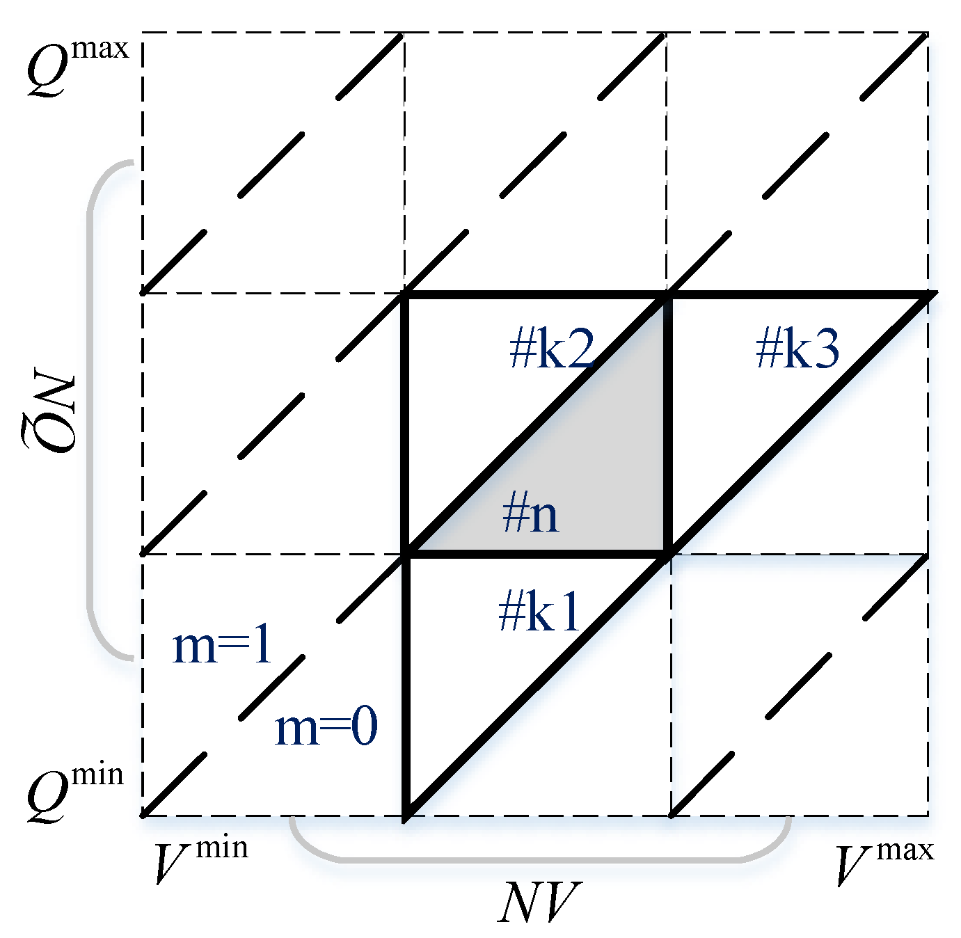
where = coefficients of the nth plane; = the subscript indices of planes; = the total number of planes; = the average storage of reservoir i in time-step t.
As illustrated in Figure 1 and detailed in our previous work [25], the domain of the hydropower output function is divided into triangular grids that have their planes, which altogether linearly concave the nonlinear hydropower output function.
Similar to the hydropower output, the capacity (5) of hydropower output can also be linearized with the same number of planes with different coefficients, expressed as:
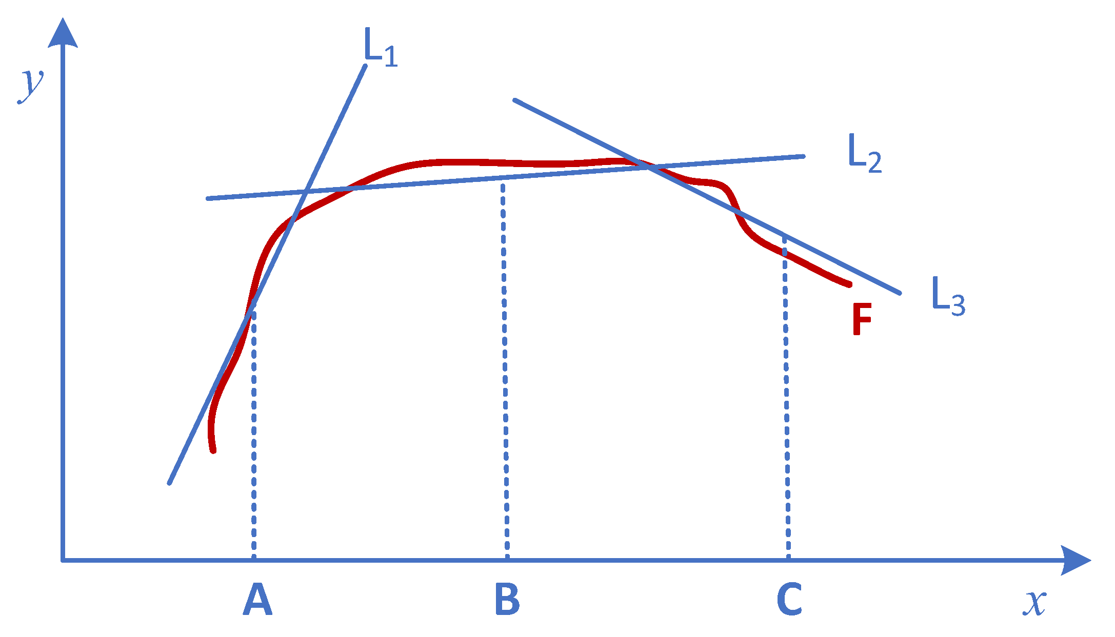
Now, the original constraints (5), (9), and (10) can be replaced with the linear constraints (12) and (13). The problem is, the hydropower curtailment in the objective does not appear in any constraint, making it impossible to minimize it as the top priority. Thus, a new constraint is created to solve this problem,
where = coefficients of the plane active in time-step t among those linearly concaving the hydropower output function of hydro-plant i. As illustrated in Figure 2, the nonlinear function (F) is linearly concaved with three lines, among which, for example, the 1st line is active at point A, the 2nd at B, and the 3rd at C.
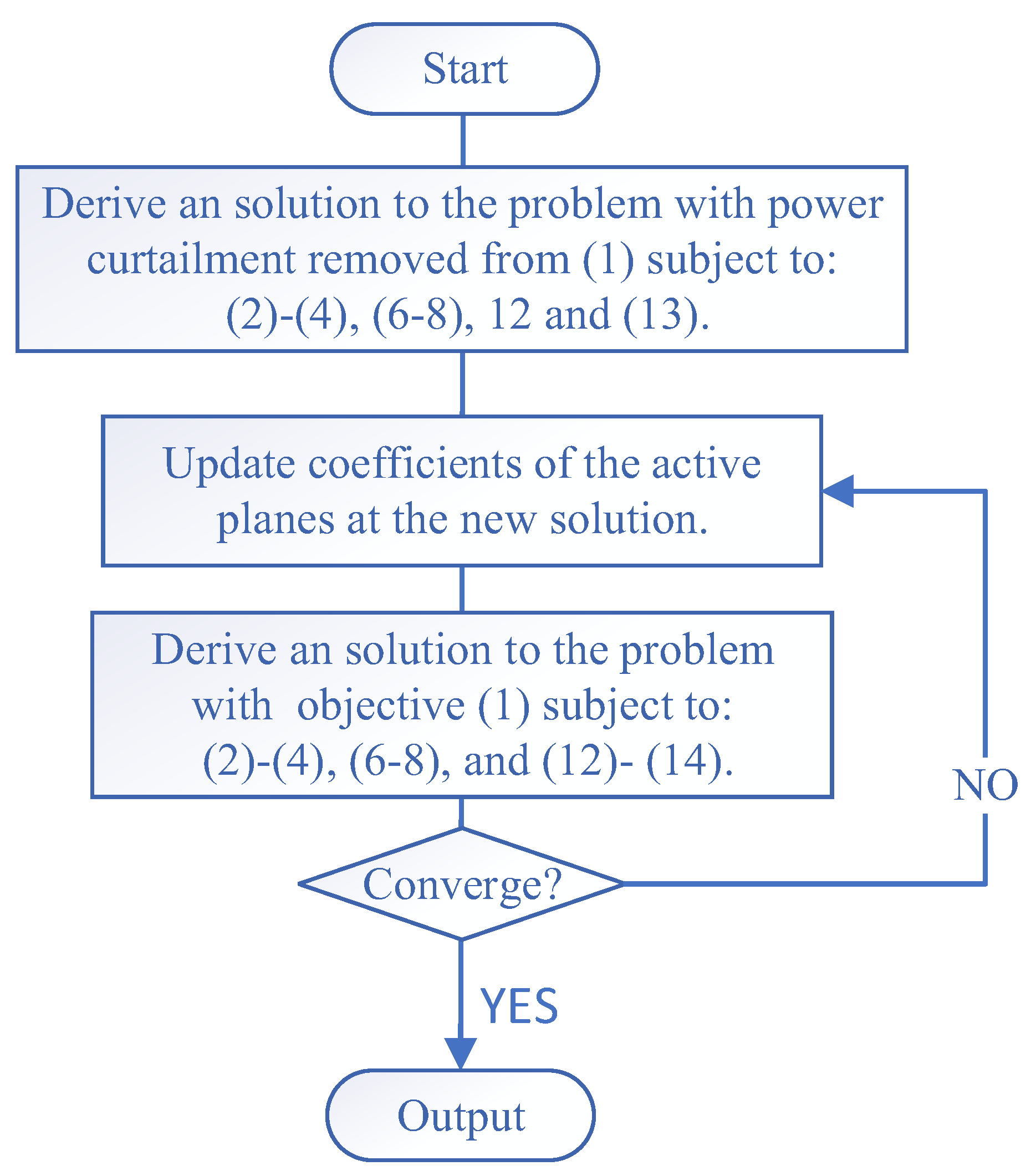
However, the active plane of a hydro-plant is different from one time-step to another and changes during the solution procedure. As demonstrated in Figure 3, this work presents a procedure to update the coefficients at the active planes in the constraint (4). The procedure derives an initial solution by solving the problem with the hydropower curtailment removed from objective (1) subject to constraints: (2)–(4), (6)–(8), (12), and (13), then updates the active planes in each time-step for all the hydro-plants based upon the new solution, and then adds the hydropower curtailment and constraint (14) into the model, which is solved again until the convergence is achieved in updating the coefficients of the active planes.
3.2. Simulation Strategy
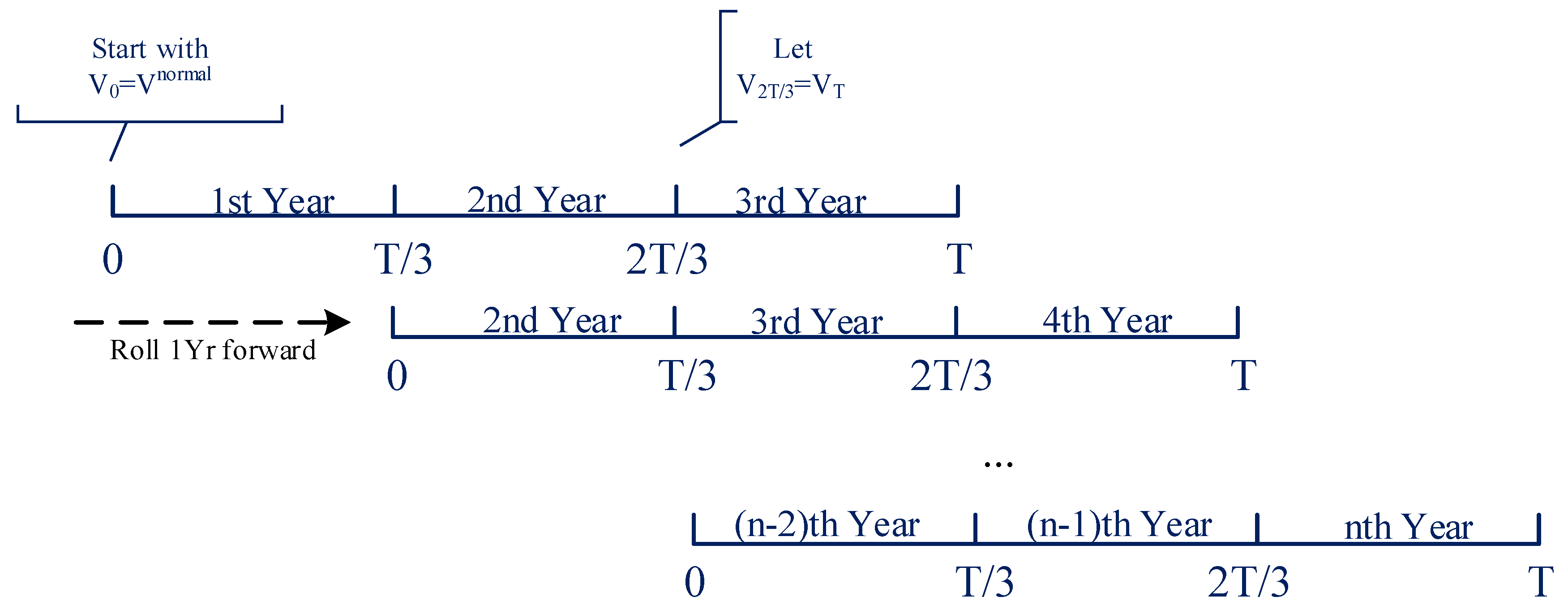
Figure 4 illustrates the rolling strategy to alleviate the dimensional difficulty in solving the model. The simulation starts with the initial storage of a reservoir assigned to a feasible storage, its normal storage, for instance. It derives the solution to the optimization problem during a scheduling horizon of three years while ensuring consistency by enforcing that the storages at the end of the 2nd and the 3rd year are equal. The simulation continues by rolling one year forward with the initial storage of a reservoir updated to that derived in the last optimization. Then, the scheduling problem will be solved again to derive a new solution. The simulation keeps rolling forward year by year until the end of the years when the historical inflows are available. After each optimization, only the results in the first year will be recorded to assess the drawdown water levels.
4. Case Studies
The model and methods will be case studied in a river in southwest China involving eleven cascaded hydropower reservoirs. The river and reservoirs are renamed to avoid unnecessary disputes beyond an academic and engineering context.
4.1. Engineering Background
The Upper Mekong River, known as the LC River in China, originates in Qinghai province, flows through China’s Qinghai, Tibet, and Yunnan provinces, and then flows out of China. It flows through Myanmar, Laos, Thailand, and Cambodia before flowing from Vietnam into the South China Sea.
The LC River has a total length of 4880 km, a drainage area of 810,000 square kilometers, and an average annual runoff of 475 billion cubic meters at its estuary, making it the most critical international river in Southeast Asia. With a hydropower potential of about 37,000 megawatts, the mainstream in the whole basin has a total drop of 5500 m, 91% of which is concentrated in the LC River. The hydropower resources that can be developed in the LC River are estimated at about 30 million kW in China, among which there are 14 cascaded hydropower stations in Yunnan Province with a total installed capacity of 25.8 million kW, accounting for about 86%, equivalent to 1.4 Three Gorges hydropower stations.
An industrial company operates the cascaded hydropower reservoirs on the LC River to maximize benefits from hydropower production under boundary conditions enforced by higher-level authorities that consider comprehensive requirements but usually do not impose monthly power demands that make hydro-plants electrically connected across multiple rivers.
By November 2019, the LC River has 11 hydro-plants under operation, among which five hydro-plants are in upstream tributaries. Table 1 summarizes the basic information of 11 cascaded hydropower reservoirs in the LC River, which will be case studied in this work over the years from 1953 to 2002 when the third-monthly historical inflows are available. The over-year OY07 and OY10 are the largest reservoirs on the river and play a critical role in coordinating their operation with the other reservoirs.
4.2. Assessment of Optional Drawdown Levels
It is assumed that both the OY07 and OY10 will draw down their water levels at the end of May proportionally over years from their flood-control to dead water levels, with the OY07 from 1236 m to 1166 m and OY10 from 804 m to 765 m. Under this assumption, eleven optional drawdown levels to be assessed for both the over-year reservoirs are generated by evenly discretizing the space between the dead and flood-control water levels into 10 intervals, as given in the 2nd and 3rd columns in Table 2, which summarizes the performances of the optional drawdown levels at the end of May, including the hydropower production and curtailment on average, as well as the full-refilling rate. A year is divided into dry and flood seasons according to the climate conditions of the basin, which may have its dry seasons in months with less rainfall if it is mainly recharged by rain, or in those with lower temperature if it is recharged primarily by the melting ice and snow on mountains. The LC River is mainly recharged by rainfall and has its dry seasons from January to May, plus November to December and the flood seasons from June to October. The reservoirs are divided into the upstream and downstream reservoirs of the OY07, which is included in the group of downstream reservoirs. The full-refilling rate is defined as the proportion of years when a reservoir can be fully refilled within a year after May. The firm third-monthly hydropower production of all the cascaded hydro-plants is the minimum over years when the operation is simulated on historical inflows.
As expected, the results in Table 2 show that targeting higher drawdown water levels at the end of May will lead to higher full-refilling rates for both the OY07 and OY10 reservoirs because there is a smaller gap of storage to be refilled to the normal capacity. As the full-refilling rate is not particularly targeted in the objective of the model, thus the reservoir does not have to refill the storage to the full capacity during a couple of years when the water level already remains at a very high level during the flood seasons. Targeting higher drawdown water levels at the end of dry seasons has, if any, very little impact on the upstream reservoirs in the hydropower curtailment due to the generating capacity, but will result in a larger curtailment in the downstream hydro-plants due to a smaller storage capacity available to reduce spillages.
The goals at the top three priorities in the model include minimizing the hydropower curtailment, the deficiency to the contracted electricity and the deviation from storage targets at the end of a scheduling horizon, which are employed to enforce constraints in year-by-year operation and will not be used to assess performances of the drawdown water levels in a long-term perspective. This work assesses the drawdown water levels at the end of dry seasons based on the total hydropower production and the firm third-monthly hydropower output. From the results in Table 2, targeting higher drawdown levels will lead to more hydropower production during the flood seasons, mainly attributable to higher water heads that contribute to higher generation efficiency of the over-year reservoirs. However, the hydropower production during dry seasons will be less when targeting higher drawdown levels at the end of dry seasons because less storage will be used for the generation, the hydropower production during a year and the firm hydropower output follow a different pattern: they go up first and then down when elevating the drawdown water levels, with the maximums occurring at the 1st, 7th, and 3rd options, respectively. Apparently, the drawdown water levels from the 3rd to 7th options are favorable for larger annual and firm hydropower productions, specifically with the OY07 from 1185 m to 1214 m and the OY10 from 774 m to 791 m.
4.3. Simulation Results of the 7th Option
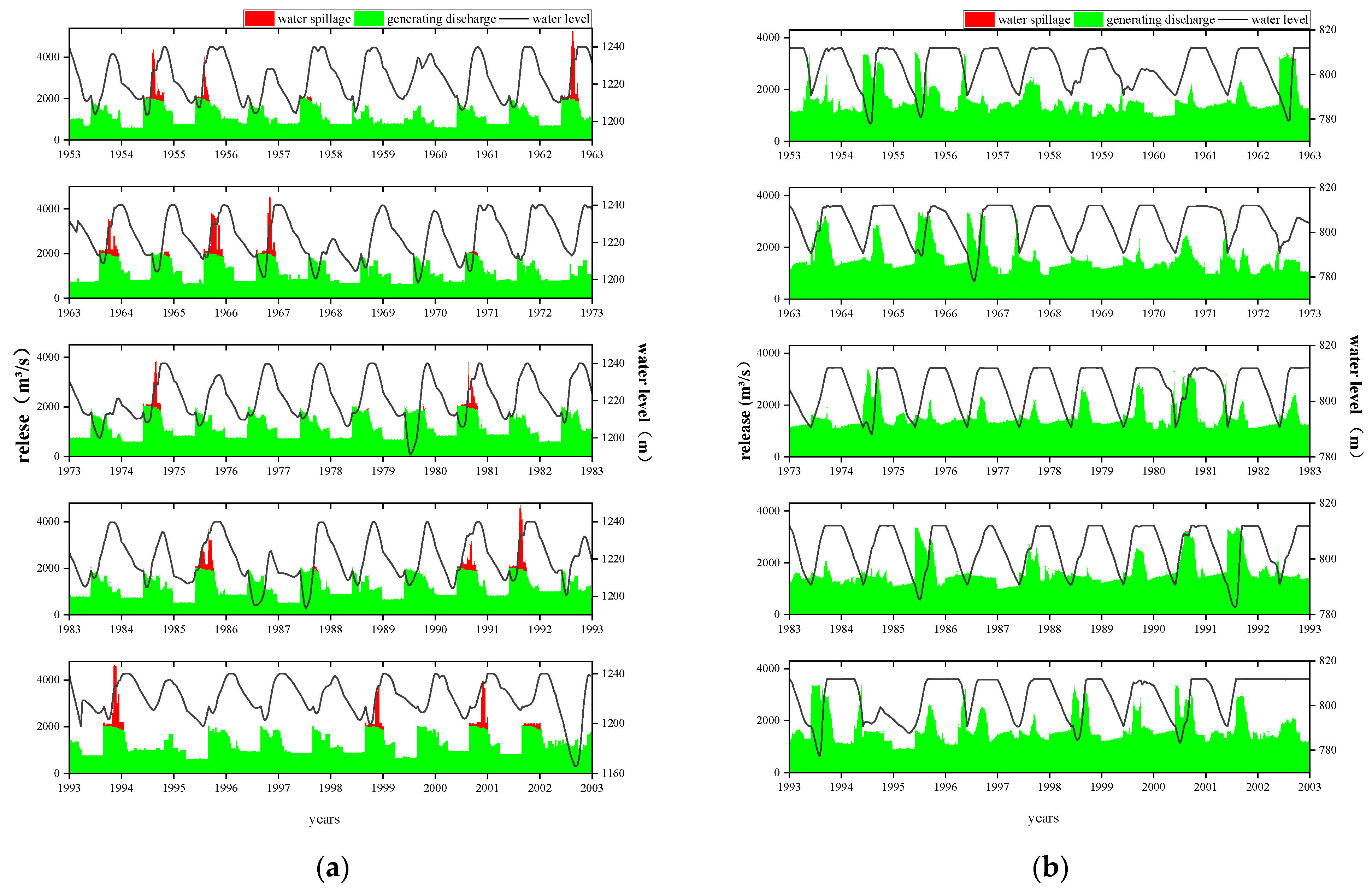
The 7th option targets the OY07 and OY10 reservoirs drawing down their forebay water levels to 1214 m and 791 m at the end of May, respectively.
Figure 5 shows the third-monthly outflows, spillages, and water levels of the OY07 and OY10 reservoirs, derived by simulating the operation of 11 hydropower cascaded reservoirs over 50 years during 1953–2002 when the local natural inflows are available. Both the over-year reservoirs share a conventional pattern in regulating their storages, drawing down, and then refilling the water level. The OY07 can fully utilize its over-year storage capacity to regulate natural runoffs, and compared with the situation without enforcing a drawdown level, it elevates its water level slightly higher at the end of May in almost every year. Consequently, it has more years when scheduled spillages occur. Impressively, the OY10 has no scheduled spillage during 50 years of simulation, demonstrating an excellent regulation capability and, at the same time, no pressure in coordinating with its downstream reservoirs for the best interests of the whole system.
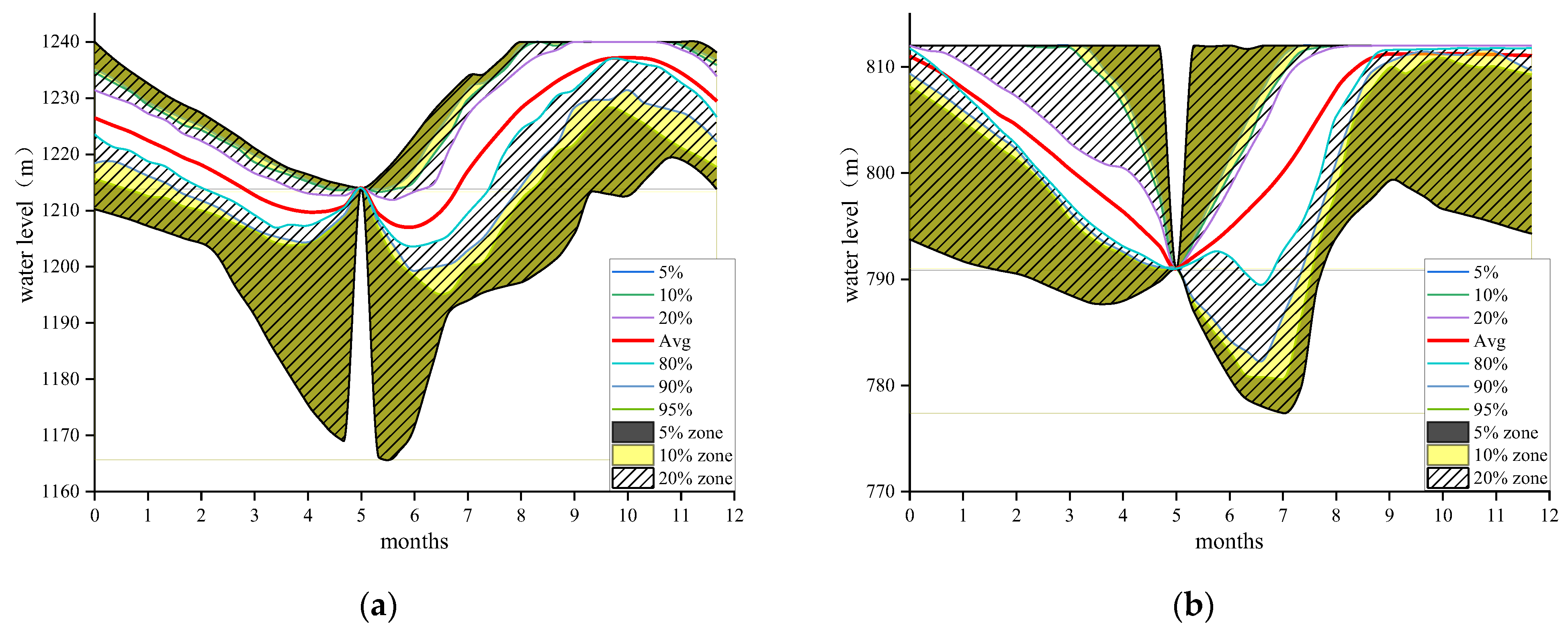
Figure 6 illustrates the distribution of the water level over the active storage space and 36 third-month (about ten days) periods in a year (12 months) for OY07 and Oy10, which are the only over-year reservoirs in the Cascade. Simulating the operation over 50 years from 1953 to 2002 gives a sample of 50 water levels in each third-month, among which the lowest, mean, and highest can be determined to provide the third-monthly minimum, mean, and maximum water levels in a year. Similarly, sorting the sample of 50 water levels in a third-month from the smallest to the largest allows us to determine different percentiles, as included in Figure 6, the 5%, 10%, 20%, 80%, 90%, and 95% percentiles, which provides facilitatory information for operators to estimate on how often the optimal water level could be in a zone. For example, it is very unlikely that the best water level will be above 5% and under the 95% percentile.
As shown in Figure 6, the OY07 and OY10 have their water levels converging to the drawdown levels targeted at the end of May. The lowest water level of the OY07 occurs in June, but in very few years, it has reached to dead water level. The OY10 has its water level reaching its normal water level mostly every year, and even its lowest in July is still far above its dead water level, indicating no pressure for the OY10 to regulate its storage capacity to meet the best interests of its downstream reservoirs.
5. Conclusions
This work aims to investigate what water levels should be drawn down at the end of dry seasons with a third-monthly hydropower scheduling model of cascaded reservoirs, which is linearized to improve the solution efficiency by linearly concaving the nonlinear hydropower output and generating capacity with planes estimated with a three-triangle based method. Assuming the boundary conditions at the end of a scheduling horizon negligibly impact the results of two years earlier than the end of the scheduling horizon, a rolling strategy is presented to simulate the reservoir operation over many years of historical inflows. Applied to 11 cascaded hydropower reservoirs in the LC River that includes two major over-year reservoirs, OY07 and OY10, the simulation over years during 1953–2002 reveals:
- (1)
- The preferential drawdown water levels should be between 1185–1214 m for the OY07 and 774–791 m for OY10 as it is in favor of both the total hydropower production and the firm third-monthly hydropower output.
- (2)
- Targeting higher drawdown levels of the OY07 and OY10 will lead to more hydropower production during the flood season, mainly attributable to higher water heads that contribute to higher generation efficiency.
- (3)
- The hydropower productions during dry season will be less when targeting higher drawdown levels. The hydropower production during the year, as well as the firm hydropower output, goes up first and then down when elevating the drawdown water levels of the over-year reservoirs, with the maximums in total hydropower production and firm hydropower output achieved by drawing the OY07 and OY10’s water levels down to (774 m, 791 m) and (1185 m, 1214 m), respectively.
- (4)
- Targeting higher drawdown water levels at the end of dry seasons has, if any, minimal impact on the upstream reservoirs of the OY07 in the hydropower curtailment due to the generating capacity, but will result in a more significant curtailment in the downstream hydro-plants due to a smaller storage capacity available to reduce spillages.
Author Contributions
Conceptualization, J.W.; Methodology, S.L.; Software, S.L.; Resources, C.Z.; Data curation, Y.W.; Writing—review & editing, X.L.; Visualization, H.Z.; Project administration, K.C. All authors have read and agreed to the published version of the manuscript.
Funding
This research received no external funding.
Data Availability Statement
The data presented in this study are available on request from the corresponding author. The data are not publicly available due to data confidentiality.
Conflicts of Interest
The authors declare no conflict of interest.
References
- Algarvio, H. The Role of Local Citizen Energy Communities in the Road to Carbon-Neutral Power Systems: Outcomes from a Case Study in Portugal. Smart Cities 2021, 4, 840–863. [Google Scholar] [CrossRef]
- Zou, C.; Xiong, B.; Xue, H.; Zheng, D.; Ge, Z.; Wang, Y.; Jiang, L.; Pan, S.; Wu, S. The role of new energy in carbon neutral. Pet. Explor. Dev. 2021, 48, 480–491. [Google Scholar] [CrossRef]
- Bamisile, O.; Wang, X.; Adun, H.; Ejiyi, C.J.; Obiora, S.; Huang, Q.; Hu, W. A 2030 and 2050 feasible/sustainable decarbonization perusal for China’s Sichuan Province: A deep carbon neutrality analysis and Energy PLAN. Energy Convers. Manag. 2022, 261, 115605. [Google Scholar] [CrossRef]
- Bilgili, M.; Bilirgen, H.; Ozbek, A.; Ekinci, F.; Demirdelen, T. The role of hydropower installations for sustainable energy development in Turkey and the world. Renew. Energy 2018, 126, 755–764. [Google Scholar] [CrossRef]
- De Souza Dias, V.; Pereira da Luz, M.; Medero, G.M.; Tarley Ferreira Nascimento, D. An Overview of Hydropower Reservoirs in Brazil: Current Situation, Future Perspectives and Impacts of Climate Change. Water 2018, 10, 592. [Google Scholar] [CrossRef] [Green Version]
- Wagner, B.; Hauer, C.; Habersack, H. Current hydropower developments in Europe. Curr. Opin. Environ. Sustain. 2019, 37, 41–49. [Google Scholar] [CrossRef]
- Li, X.; Chen, Z.; Fan, X.; Cheng, Z. Hydropower development situation and prospects in China. Renew. Sustain. Energy Rev. 2018, 82, 232–239. [Google Scholar] [CrossRef]
- Dogmus, Ö.C.; Nielsen, J.Ø. Is the hydropower boom actually taking place? A case study of a South East European country, Bosnia and Herzegovina. Renew. Sustain. Energy Rev. 2019, 110, 278–289. [Google Scholar] [CrossRef]
- Meng, Y.; Liu, J.; Leduc, S.; Mesfun, S.; Kraxner, F.; Mao, G.; Qi, W.; Wang, Z. Hydropower production benefits more from 1.5 °C than 2 °C climate scenario. Water Resour. Res. 2020, 56, e2019WR025519. [Google Scholar] [CrossRef]
- Madani, K.; Lund, J.R. Modeling California’s high-elevation hydropower systems in energy units. Water Resour. Res. 2009, 45, W09413. [Google Scholar] [CrossRef]
- Lu, S.; Shang, Y.; Li, W.; Peng, Y.; Wu, X. Economic benefit analysis of joint operation of cascaded reservoirs. J. Clean. Prod. 2018, 179, 731–737. [Google Scholar] [CrossRef]
- Berga, L. The role of hydropower in climate change mitigation and adaptation: A review. Engineering 2016, 2, 313–318. [Google Scholar] [CrossRef] [Green Version]
- Oven-Thompson, K.; Alercon, L.; Marks, D.H. Agricultural vs. hydropower tradeoffs in the operation of the High Aswan Dam. Water Resour. Res. 1982, 18, 1605–1613. [Google Scholar] [CrossRef]
- Farfan, J.; Breyer, C. Combining floating solar photovoltaic power plants and hydropower reservoirs: A virtual battery of great global potential. Energy Procedia 2018, 155, 403–411. [Google Scholar] [CrossRef]
- Hirth, L. The benefits of flexibility: The value of wind energy with hydropower. Appl. Energy 2016, 181, 210–223. [Google Scholar] [CrossRef]
- Wang, J.; Huang, W.; Ma, G.; Wang, Y. Determining the optimal year-end water level of a multi-year regulating storage reservoir: A case study. Water Sci. Technol. Water Supply 2016, 16, 284–294. [Google Scholar] [CrossRef]
- Jiang, Z.; Song, P.; Liao, X. Optimization of Year-End Water Level of Multi-Year Regulating Reservoir in Cascade Hydropower System Considering the Inflow Frequency Difference. Energies 2020, 13, 5345. [Google Scholar] [CrossRef]
- Liu, J.; Huang, C.H.; Zeng, G.Z. Comparative analysis of year-end water level determining methods for cascade carryover storage reservoirs. In Proceedings of the IOP Conference Series: Earth and Environmental Science, Zvenigorod, Russia, 4–7 September 2017; IOP Publishing: Qingdao, China, 2017; Volume 82, p. 012060. [Google Scholar] [CrossRef] [Green Version]
- Zhang, Z.; Zhang, S.; Geng, S.; Jiang, Y.; Li, H.; Zhang, D. Application of decision trees to the determination of the year-end level of a carryover storage reservoir based on the iterative dichotomizer 3. Int. J. Electr. Power Energy Syst. 2015, 64, 375–383. [Google Scholar] [CrossRef]
- Celeste, A.B.; Billib, M. Evaluation of stochastic reservoir operation optimization models. Adv. Water Resour. 2009, 32, 1429–1443. [Google Scholar] [CrossRef]
- De Souza Zambelli, M.; Martins, L.S.; Soares Filho, S. Advantages of deterministic optimization in long-term hydrothermal scheduling of large-scale power systems. In Proceedings of the 2013 IEEE Power & Energy Society General Meeting, Vancouver, BC, Canada, 21–25 July 2013; IEEE: New York, NY, USA, 2013; pp. 1–5. [Google Scholar] [CrossRef]
- Allen, R.B.; Bridgeman, S.G. Dynamic programming in hydropower scheduling. J. Water Resour. Plan. Manag. 1986, 112, 339–353. [Google Scholar] [CrossRef]
- Zambelli, M.S.; Soares, S.; da Silva, D. Deterministic versus stochastic dynamic programming for long term hydropower scheduling. In Proceedings of the 2011 IEEE Trondheim PowerTech, Trondheim, Norway, 19–23 June 2011; IEEE: New York, NY, USA, 2011; pp. 1–7. [Google Scholar] [CrossRef]
- Kang, C.; Guo, M.; Wang, J. Short-term hydrothermal scheduling using a two-stage linear programming with special ordered sets method. Water Resour. Manag. 2017, 31, 3329–3341. [Google Scholar] [CrossRef]
- Zheng, H.; Feng, S.; Chen, C.; Wang, J. A new three-triangle based method to linearly concave hydropower output in long-term reservoir operation. Energy 2022, 250, 123784. [Google Scholar] [CrossRef]
Figure 1.
Triangulation of the domain of the power output function.

Figure 2.
Illustration of active lines.

Figure 3.
Procedure to update the active planes.

Figure 4.
The rolling strategy in simulations over many years.

Figure 5.
The third-monthly results by simulating the 8th option over the years 1953–2002. (a) OY07; (b) OY10.
Figure 5.
The third-monthly results by simulating the 8th option over the years 1953–2002. (a) OY07; (b) OY10.

Figure 6.
The distribution of the water level over space and time within a year. (a) OY07; (b) OY10.
Figure 6.
The distribution of the water level over space and time within a year. (a) OY07; (b) OY10.


Table 1.
Profile of the cascaded reservoirs in the Test River.
| Number | Name | Annual Inflow (m3/s) | Installed Capacity (MW) | Dead Water Level (m) | Normal Water Level (m) | Operability |
|---|---|---|---|---|---|---|
| 1 | D01 | 744 | 990 | 1901 | 1906 | Daily |
| 2 | D02 | 758 | 420 | 1814 | 1818 | Daily |
| 3 | S03 | 902 | 1900 | 1586 | 1619 | Seasonal |
| 4 | D04 | 923 | 920 | 1472 | 1477 | Daily |
| 5 | W05 | 960 | 1400 | 1398 | 1408 | Weekly |
| 6 | D06 | 1010 | 900 | 1303 | 1307 | Daily |
| 7 | OY07 | 1210 | 4200 | 1166 | 1240 | Over-year |
| 8 | S08 | 1230 | 1670 | 988 | 994 | Seasonal |
| 9 | S09 | 1330 | 1350 | 887 | 899 | Seasonal |
| 10 | OY10 | 1740 | 5850 | 765 | 812 | Over-year |
| 11 | W11 | 1810 | 1750 | 591 | 602 | Weekly |
Table 2.
The performances of optional drawdown levels at the end of May.
| Option | Water Level (m) | Hydropower Production (TW) | Curtailment (TW) | Full-Refilling Rate | ||||||
|---|---|---|---|---|---|---|---|---|---|---|
| OY07 | OY10 | Annu. | Dry | Flood | Firm | Up | Down | OY07 | OY10 | |
| 1 | 1166 | 765 | 102.17 | 48.63 | 53.54 | 1.54 | 4.86 | 0.76 | 38% | 54% |
| 2 | 1176 | 770 | 102.9 | 48.23 | 54.67 | 1.56 | 4.85 | 0.87 | 40% | 64% |
| 3 | 1185 | 774 | 103.54 | 47.51 | 56.03 | 1.56 | 4.85 | 1.06 | 46% | 76% |
| 4 | 1193 | 779 | 104.06 | 46.87 | 57.19 | 1.54 | 4.85 | 1.30 | 52% | 90% |
| 5 | 1201 | 783 | 104.47 | 46.23 | 58.24 | 1.52 | 4.85 | 1.54 | 64% | 92% |
| 6 | 1207 | 787 | 104.75 | 45.43 | 59.33 | 1.50 | 4.85 | 1.80 | 64% | 98% |
| 7 | 1214 | 791 | 104.82 | 44.09 | 60.73 | 1.45 | 4.85 | 2.12 | 78% | 100% |
| 8 | 1219 | 794 | 104.64 | 42.53 | 62.12 | 1.38 | 4.85 | 2.59 | 82% | 100% |
| 9 | 1225 | 798 | 104.32 | 40.88 | 63.45 | 1.31 | 4.85 | 2.59 | 88% | 100% |
| 10 | 1231 | 801 | 103.74 | 39.09 | 64.65 | 1.22 | 4.85 | 3.86 | 94% | 100% |
| 11 | 1236 | 804 | 103.24 | 37.39 | 65.84 | 1.14 | 4.85 | 4.56 | 100% | 100% |
Note: Annu. = annual; Dry & Flood = during dry & flood seasons, respectively; Up & Down = upstream &downstream reservoirs, respectively.
Disclaimer/Publisher’s Note: The statements, opinions and data contained in all publications are solely those of the individual author(s) and contributor(s) and not of MDPI and/or the editor(s). MDPI and/or the editor(s) disclaim responsibility for any injury to people or property resulting from any ideas, methods, instructions or products referred to in the content. |
© 2023 by the authors. Licensee MDPI, Basel, Switzerland. This article is an open access article distributed under the terms and conditions of the Creative Commons Attribution (CC BY) license (https://creativecommons.org/licenses/by/4.0/).
Share and Cite
MDPI and ACS Style
Liu, S.; Luo, X.; Zheng, H.; Zhang, C.; Wang, Y.; Chen, K.; Wang, J. Investigation on Water Levels for Cascaded Hydropower Reservoirs to Drawdown at the End of Dry Seasons. Water 2023, 15, 362. https://doi.org/10.3390/w15020362
AMA Style
Liu S, Luo X, Zheng H, Zhang C, Wang Y, Chen K, Wang J. Investigation on Water Levels for Cascaded Hydropower Reservoirs to Drawdown at the End of Dry Seasons. Water. 2023; 15(2):362. https://doi.org/10.3390/w15020362
Chicago/Turabian StyleLiu, Shuangquan, Xuhan Luo, Hao Zheng, Congtong Zhang, Youxiang Wang, Kai Chen, and Jinwen Wang. 2023. "Investigation on Water Levels for Cascaded Hydropower Reservoirs to Drawdown at the End of Dry Seasons" Water 15, no. 2: 362. https://doi.org/10.3390/w15020362
Note that from the first issue of 2016, this journal uses article numbers instead of page numbers. See further details here.