Extending the Overlay and Index: A Simple Method for Assessing Aquifer Vulnerability in a Combined Vadose Zone—Groundwater Flow System

Abstract

This work extends the overlay and index methods for intrinsic groundwater vulnerability, that typically involve the soil surface and the vadose zone, to groundwater (saturated) transport. The method is “hybrid” as it combines the standard overlay and index methods with a simplified process-based approach for the groundwater component. For the latter, we make use of concept and methodologies based on geomorphological analysis, employing tools that are generally implemented in Geographic Information Systems (GIS). The proposed method is based on a simple probabilistic analysis, in which the overlay and index method (that can be any) provides the probability that the contamination reaches the groundwater through the vadose zone, while the probability that the contaminant reaches a generic location in the groundwater system is determined by analyzing the groundwater streamlines. The analysis leads to the definition of the combined vulnerability index $\upsilon$, that takes care of both transport in the vadose zone and the aquifer. The method is applied to a groundwater catchment in the Campania region, Southern Italy. The method is simple and effective in assessing aquifer vulnerability in a combined vadose zone—groundwater flow system, useful for preliminary, screening analysis of the intrinsic aquifer vulnerability.

1. Introduction

Groundwater is the most important source of freshwater worldwide, for both humans and ecosystems. The quality of groundwater is currently under threat in many areas of the world because of several different factors, including the development and increase of human settlements, the industrial and farming activities, the release (accidental or not) of several chemical products [1]; new products are introduced every year in the environment, polluting the groundwater resource, with consequences to the human health and the ecosystems that are still unknown. Protection of groundwater is therefore necessary for a correct management of the resource, and the first step is the assessment of its vulnerability after potential contamination.

Assessing the vulnerability of groundwater to contamination is an important topic that has been the subject of intensive research in the last few decades. The complexity of groundwater systems, which are inherently heterogeneous, three-dimensional and connected with surface water, together with the hydrological processes taking place in them, namely, flow and contaminant transport in the vadose zone and in the aquifer, make the assessment of vulnerability an extremely difficult task.

For the above reasons, different approaches have been followed in the past to provide reliable groundwater vulnerability assessments, with different level of complexity and approximation. The body of scientific work published on the matter in the years is truly impressive, and a few review on the subject have tried to summarize and organize the main achievements; among which we cite the review by Gogu and Dassargues [2], Sorichetta et al. [3], Wachniew et al. [4], Iván and Mádl-Szőnyi [5], Barbulescu [6], Goyal et al. [7]. With some exceptions, most of the reviews are focused on the overlay and index methods, which are probably among the most popular for the assessment of groundwater vulnerability.

The aquifer vulnerability is usually distinguished between “intrinsic” and “specific” [8]: while the former accounts for the hydrological and geological characteristics of an area, being independent of the specific nature of contaminants, the latter refers to a single or a group of specific contaminants, considering their properties and their transformations. In this work we focus on intrinsic vulnerability.

A few approaches can be followed for the vulnerability assessment, which can be categorized as follows [9,10]:

• Overlay and index methods, which are of an empirical nature, relying mostly on hydrogeological parameters: They implicitly consider only the unsaturated zone, without taking into account the transport processes within the saturated zone; examples of such methods are the widely popular DRASTIC [11], SINTACS [12], EPIK [13], GOD [14], and AVI [15], to mention a few.
• Process-based methods, which explicitly solve the flow and transport equations (unsaturated and saturated) to predict the fate of the contamination: Although such methods provide a physics-based, quantitative assessment of vulnerability, they are usually more complex and require more data and computational resources than the index methods. The main advantage is that both the vadose zone and the saturated flow are jointly considered, providing a more comprehensive and sound assessment of vulnerability.
• Statistical methods, which involve some probabilistic method applied to the available data, with different degrees of complexity.
• Hybrid methods, which combine some or all of the above methods.

While the overlay and index methods are extremely simple to apply, which is among the reasons of their success, they completely neglect the groundwater (saturated flow) component since they do not consider the fate of a contaminant once it has reached the groundwater; the latter process however, is of paramount importance when assessing vulnerability. This limitation is not present in the process-based methods, which however are much more complex and demanding in terms of data and computational resources, and hence less popular.

The scope of the present work is to provide a framework for bridging the above gap, i.e., assessing aquifer intrinsic aquifer vulnerability that is based on the simple overlay and index methods but attempts at introducing the important groundwater component, with a level of complexity that is comparable to the index methods. Thus, the novelty of the proposed method is to implicitly consider the combined vadose zone - groundwater system, keeping the simplicity and the knowledge/experience accumulated on the index methods over the years. The proposed method can be considered as “hybrid”, in the terminology of Taghavi et al. [10], as it combines the overlay and index method with a simplified process-based approach for the groundwater component; for the latter we make use of concept and tools based on geomorphological analysis. We note that most of the hybrid methods available are a combination of index and statistical methods [10], and we are not aware of a combination of methods similar to the one proposed here.

The organization of the paper is as follows. The methodological framework is introduced first, together with the concept of combined vulnerability. The suggested implementation, based on concepts borrowed from geomorphology, is explained and detailed. The method is applied to the case study of the Campania Plain, with a discussion of results. A set of Conclusions closes the paper.

2. Methodological Framework and the Definition of Combined Vulnerability

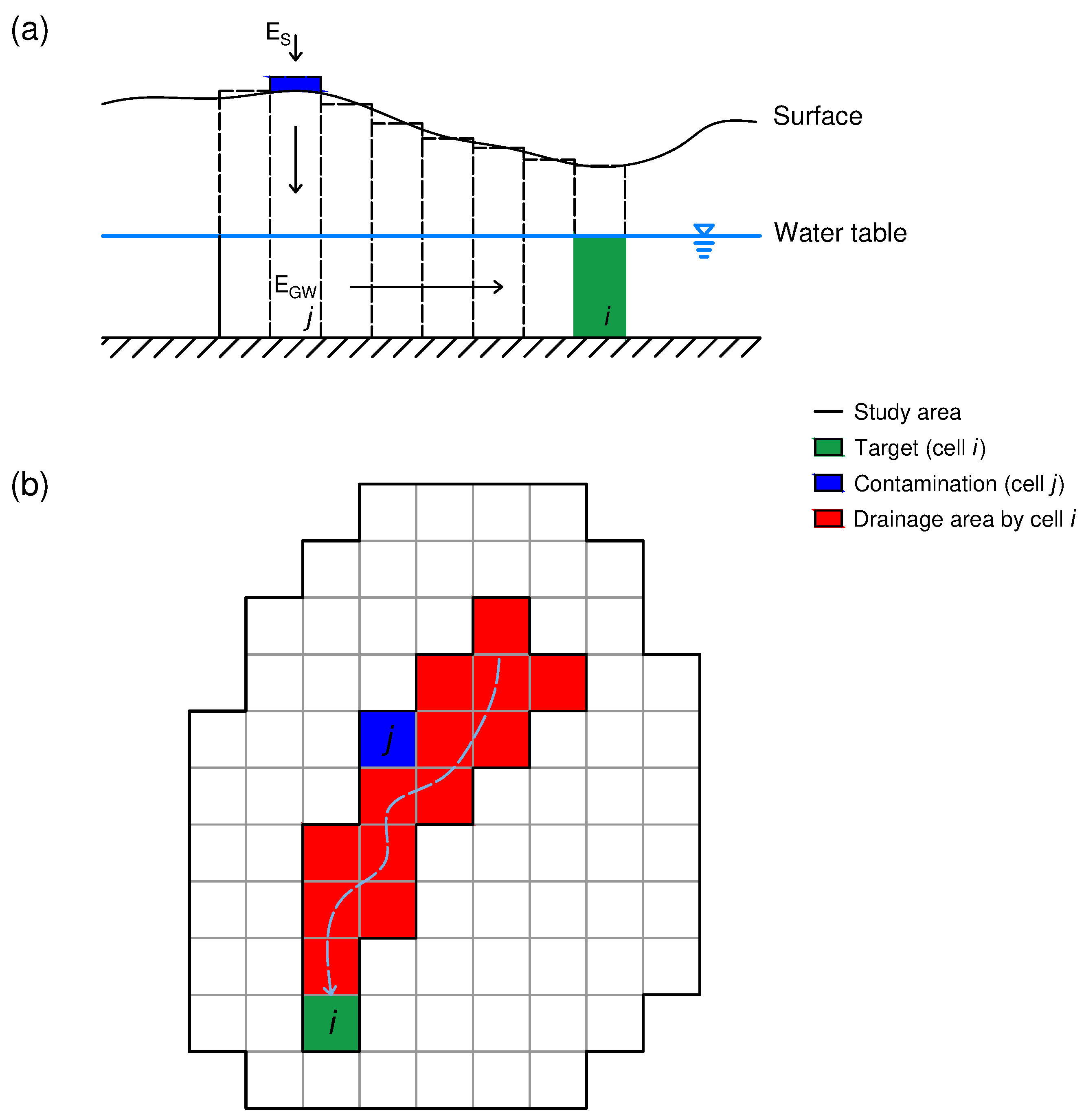
We focus on the intrinsic vulnerability of the aquifer and follow the path of a generic contaminant released at the surface, along a Lagrangian fashion. The conceptual model adopted here is the one depicted in Figure 1a, where the contaminant trajectory follows first a vertical path along the soil and the vadose zone (unsaturated porous medium) and then moves sub-horizontally along the aquifer (saturated porous medium), to reach a specific control plane or target. Groundwater flow is assumed as steady. The setup is similar to the one adopted in Russo and Fiori [16], although the analysis is much simplified here. In particular, we make use of the well known overlay and index methods for assessing the vulnerability related to the vadose zone.

The aquifer in the area of interest is divided in N cells, of equal size (see Figure 1b). For each aquifer cell a vulnerability index V is provided, along any of the several overlay and index methods available. For each cell i a groundwater subcatchment can be defined, collecting and delivering recharge by rainfall to i. We denote as $E_S$ and $E_{GW}$ the event of contamination occurring at the surface and in the groundwater, respectively. $P\left(E_S\right)$ is the probability that a contaminant is released at the generic cell at the surface (hereinafter P denotes probability). We assume that the contamination occurs only in one cell within the groundwater subcatchment feeding cell i, e.g., in the case of an accidental spill. In turn, $P(E_{GW}\mid E_S)$ is the probability to have an event of contamination in the groundwater conditional to a contamination at the surface; such probability depends on the transport processes in the vadose zone and its structural/hydraulic features (thickness, conductivity, etc.), not on transport features pertaining to a particular contaminant (e.g., retardation or decay) as we focus on the intrinsic vulnerability. We assume here that $P(E_{GW}\mid E_S)$ is proportional to the vulnerability V, as calculated by the index method, which indeed loosely represents the “relative probability that troublesome concentrations of contaminants reach the saturated zone” [2], i.e., considering only the soil and the unsaturated zone. Hence we can write for each cell

$$P(E_{GW}\mid E_S)=f\left(V\right)$$

(1)

where $f\left(V\right)$ is a function that converts vulnerability into a probability, which can be of any type, as function of the index method adopted; since the rather empirical nature of the index methods such function has also some degree of arbitrariness. Assuming for simplicity a linear function $f\left(V\right)=\xi V$ we have

$$P(E_{GW}\mid E_S)=\xi V$$

(2)

with $\xi$ a scaling factor such as to convert vulnerability into a probability (for instance $\xi =V_{max}^{-1}$ with $V_{max}$ a given maximum value for vulnerability).

By the definition of conditional probability, the probability that contamination occurs at both surface and groundwater $\pi =P(E_S\cap E_{GW})$ is

$$\pi =P(E_{GW}\mid E_S)P\left(E_S\right)=\xi Vp$$

(3)

with $p=P\left(E_S\right)$ the probability of contamination event at the surface. With N the total number of aquifer cells in the domain under consideration, a uniform probability $P\left(E_S\right)$ would give $p=1/N$; otherwise, p may reflect the presence of potential sources of contamination (industries, agricultural activities, urban areas, etc.), that however may be also partially included in the vulnerability index adopted. The contamination events at the cells are mutually exclusive, and as a consequence ${\sum }_{i=1}^N{p}_i=1$.

We move now to the groundwater component. As mentioned above, each groundwater cell i drains a subcatchment upstream of it (Figure 1b), characterized by a number of aquifer cells $N_i$; a contamination in any of those cells will reach cell i, with different travel times, increasing its vulnerability. According to (3), each of the $N_i$ cells has a given probability of contamination ${\pi }_j=\xi V_j{p}_j(j=1,\cdots ,N_i)$, where the index j refers to all the $N_i$ cells upstream of i. The total probability of contamination at cell i, due to contamination and infiltration over any of the $N_i$ cells upstream and subsequent transport by groundwater, is equal to the total probability

$${\Pi }_i=P(E_{GW,1}\cup E_{GW,2}\cup \dots \cup E_{GW,N_i})$$

(4)

where the generic event $E_{GW,j}$ occurs at cell j within the $N_i$ cells drained by cell i. In words, Equation (4) is the probability that a contamination occurs in the groundwater, at the generic cell i, coming from any of the aquifer cells upstream that deliver water (and contaminant) to i; such probability is a measure of vulnerability of the cell under consideration. Since the events $E_{G{W}_j}$ are mutually exclusive (there is only one cell contaminated), the total probability (4) writes as

$${\Pi }_i=\sum _{j=1}^{N_i}{\pi }_j=\xi \sum _{j=1}^{N_i}{V}_j{p}_j$$

(5)

Assuming a uniform probability of contamination at the surface, e.g., $p_j=p=const=1/N$, the total vulnerability at cell i is equal to the sum of vulnerabilities of all the cells drained by i. With the above steps, the following vulnerability index is here defined

$${\upsilon }_i=\frac{{\Pi }_i}{p\xi }=\sum _{j=1}^{N_i}{V}_j$$

(6)

The above is coined here as combined vulnerability. Summarizing, the combined vulnerability ${\upsilon }_i$ (6) represents the intrinsic vulnerability of the generic cell i to contamination, combining both transport in the vadose zone and in the groundwater; the contamination occurs at a (random) cell upstream of i. Along Formula (6) the combined vulnerability is simply the sum of the vulnerability index of the cells upstream of each cell of the domain of interest.

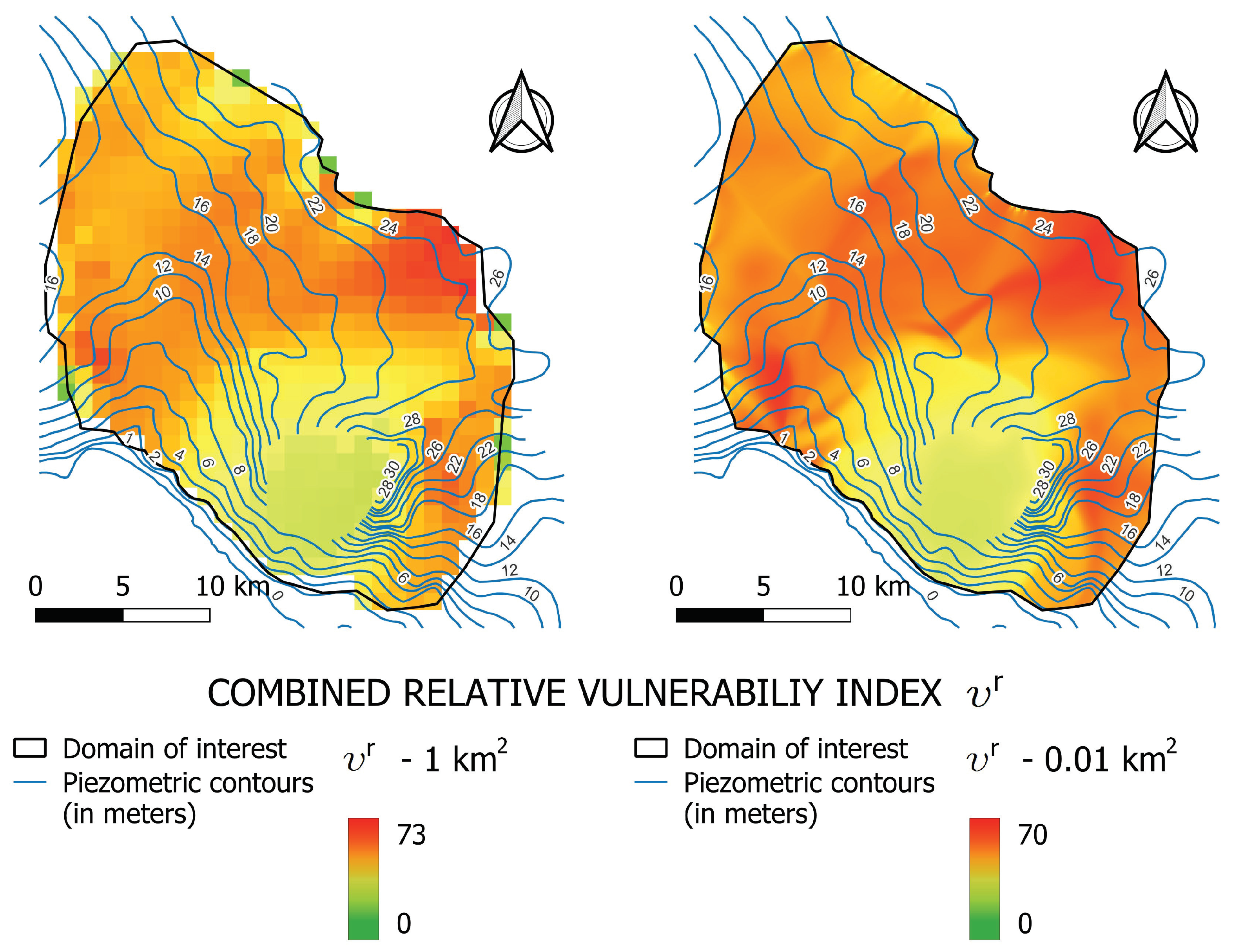
The definition (6) factors out the term $p\xi$; as a matter of fact, a precise quantification of both p and $\xi$ is not needed if the concept of vulnerability is employed in a relative manner, e.g., by assessing whether a region is more vulnerable that another, as typically done with the index methods. As a consequence, the combined vulnerability will depend on the level of discretization adopted, with larger values pertaining to finer grids. Thus, comparison of vulnerabilities among different geographic areas should be performed with the same level of discretization.

An additional vulnerability index, still intrinsic, is also introduced here; it also considers the dilution processes occurring in the subsurface. Because of recharge from rainfall, each cell i has a groundwater discharge roughly proportional to the drained area upstream, which in turn is proportional to $N_i$. Thus, an alternative measure of vulnerability that partially accounts for local dilution can be defined by dividing $\upsilon$ by the groundwater discharge, i.e., $N_i$, as follows

$${\upsilon }_i^r=\frac{{\upsilon }_i}{N_i}=\frac{1}{N_i}\sum _{j=1}^{N_i}{V}_j$$

(7)

The above is defined as the combined relative vulnerability, and it may provide an additional piece of information in cases when the dilution of contaminant operated by the groundwater system is an important component, besides the mere occurrence of the contamination, which in turn is assessed by $\upsilon$. According to Equation (7), the combined relative vulnerability is the average of the vulnerabilities of the cells upstream i.

Besides the vulnerability V, the proposed method requires the definition of the $N_i$ cells upstream each location i. The groundwater streamlines covering the entire hydrogeologic basin are therefore needed, which can be obtained after knowledge of the piezometric head. Hence, an important requisite is the complete knowledge of the piezometric contour lines, from which the subsurface drainage area can be obtained for every location. The piezometric contours are usually found in hydrogeological maps and are characterized by different levels of approximation, for instance being derived from spatial interpolation of point measurements, from calibration of numerical models or from simpler, empirical analyses, also depending on the data availability; in some cases, e.g., for shallow aquifers, the topography can be adopted as an approximation of the water table [17]. Once the piezometric contours are available, even in an approximate form, the streamlines (normal to the contours) are easily obtained, and so are the groundwater subcatchments drained by each cell i of the domain.

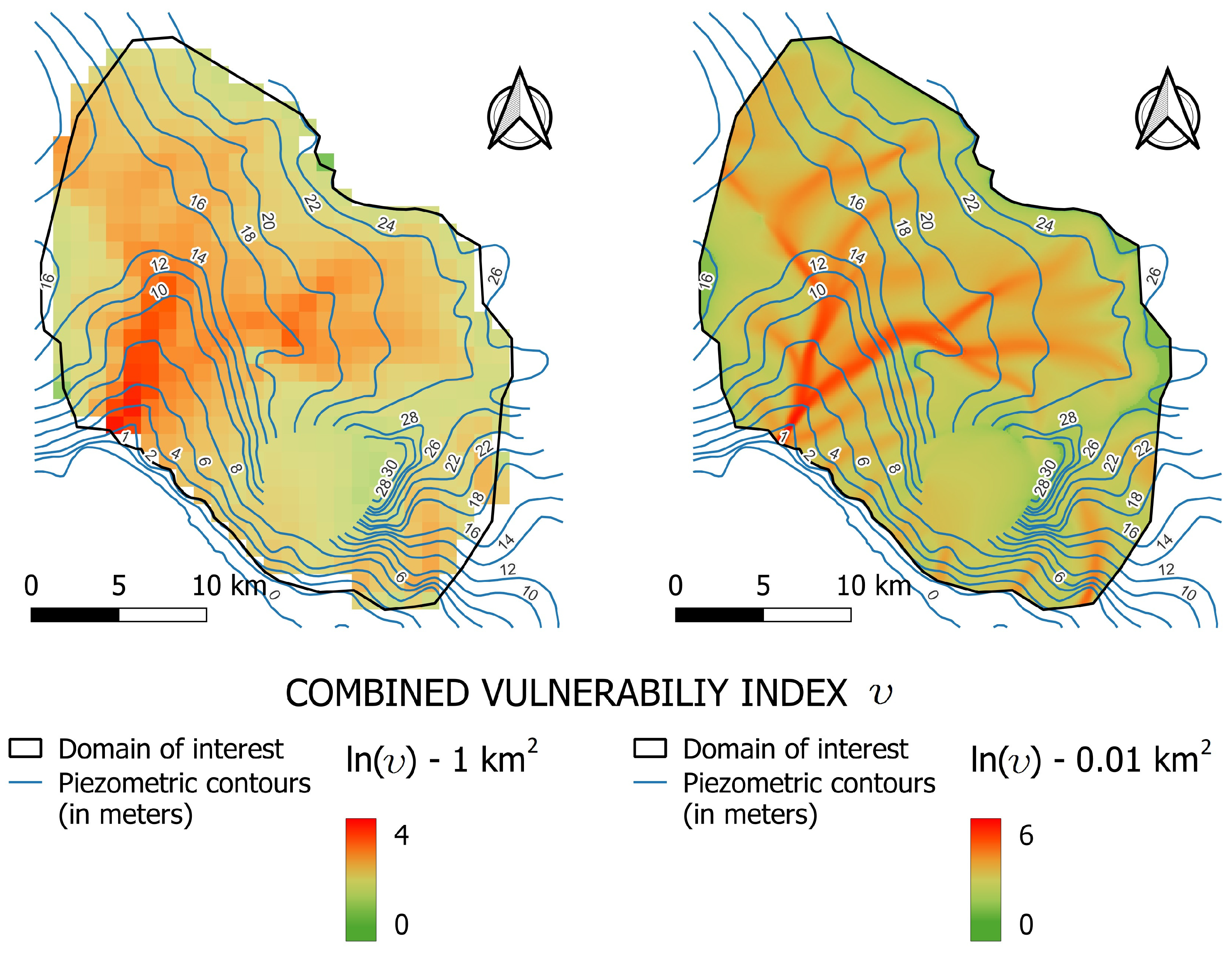
We note that the vulnerability $\upsilon$ depends on the size of the cells, which should be compatible with the discretization adopted for the calculation of V by the index method. A coarser grid (lower resolution) typically increases the average size of the groundwater subcatchments and decreases their number. Instead, the size of subcatchments decreases with finer grids (higher resolution); in the extreme, theoretical case of infinitesimal cells, the subcatchment coincides with the upstream segment of the streamline passing through i. Hence, the resolution has an impact on the channeling effects and the size groundwater subcatchments, with a greater flow concentration in smaller parts of the domain (“hot spots”) when adopting higher resolutions.

A finer grid may also raise or exacerbate possible inconsistencies of the piezometric head; because of the spatial interpolation or other methods from which the piezometric head is derived, the resulting piezometric field may not completely fulfill the flow equations (continuity and Darcy), such as to bring issues such as crossing of streamlines that are otherwise not permitted (except along sources or sinks). Therefore, the size of the cells cannot be too small, a requirement that is shared by the overlay and index methods.

Summarizing, the size of the cell results after a trade-off between the need of a detailed representation of vulnerability, the support scale of the index-based vulnerability V adopted, and the accuracy of the piezometric contours. Generally speaking, it seems reasonable to keep the same discretization adopted for the calculation of the index V also for the calculation of the combined vulnerability $\upsilon$.

In the following section we show how to implement the method in a simple and effective manner by using well-known geomorphology-based tools, within a GIS environment.

3. Implementation by Geomorphological Methods

The proposed method can be easily implemented by employing the nowadays standard and widely available tools developed in the area of geomorphological analysis, well known in the literature (see [18]). In the geomorphological width-function-based IUH approach the driving force of water is gravity, i.e., elevation. Employing a Digital Elevation Map (DEM), such approaches allow evaluating a series of important attributes related to river networks and subcatchments, e.g., river network extraction, basin delineation and others. The typical steps of a geomorphological analysis for processing DEM are: (i) pit filling, (ii) calculation of flow directions and (iii) flow accumulation. The latter provides, for each point within the catchment, the (surface) drainage area closed at that point.

Groundwater is ruled by piezometric head instead of elevation, but the problem of the determination of flow directions is analog to the one for surface water; instead of being normal to elevation, streamlines are normal to the piezometric head. Hence, the spatial analysis and related tools can be effectively employed by substituting piezometric head instead of elevation. Hence, the standard steps reproduced above can be adopted, with a few noteworthy differences, as follows.

First, the pit filling, that is required in surface water in order to avoid endorheic basins that are often induced by errors in the DEM, is not recommended for groundwater. In fact, local piezometric minima are often present in aquifers (e.g., wells or springs) and their artificial removal may leads to mistakes in the subcatchment delineation, and then in the identification of vulnerability prone areas.

Second, a unique determination of the flow directions for a given cell may not be appropriate in groundwater, for which the spatial aggregation of the piezometric head in cells (typically of large size) may easily lead to several possible flow directions; one example is a cell from which the piezometric head diverges downstream, such that the cell delivers water in more than one direction. Thus, techniques such as D8 [19] or similar may not be a good choice as they derive an unique flow direction pattern. Instead, the Multiple Flow Directions (MFD) method [20] allows for multiple flow directions of flow, which seems more in line with what happens with the groundwater flow aggregated over (typically large) spatial scales. While the MFD method may be more suited to the case analyzed here, the particular choice for the flow direction method does not significantly affect the results, which are mostly determined by the piezometric contours and the particular choice for the overlay and index method.

The use of the geomorphological methods, fed by the piezometric head instead of the DEM, allows the immediate calculation of the combined vulnerability (6), and same for its relative variant (7). In fact, Formula (6) corresponds exactly to the definition of weighted flow accumulation (6), in which the weights are provided by the grid of the vulnerability V, calculated by the overlay and index method. In turn, the number of upstream cells $N_i$ corresponds to the flow accumulation (without weight), allowing for the calculation of the specific combined vulnerability (7).

We emphasize that the suggested analysis requires that the study area is carefully defined as the vulnerabilities ${\upsilon }_i$ and ${\upsilon }_i^r$ embed information related to the whole drainage area upstream each cell. Therefore, it is fundamental to include the whole drainage catchment upstream each cell, and this is done by extending the domain size up to the flow divides.

The above steps are routinely implemented in most GIS platforms; in this work we have used the popular QGIS software [21]. In particular, the routines that have been employed are Catchment Area to calculate the subcatchment areas from the piezometric head, with the use of index-based vulnerability as weight and setting multiple flow direction as drainage direction. In the end, through the use of Raster Calculator, the combined vulnerability index $\upsilon$ is obtained by dividing the entire map with the cell area. We remind that the data required by the procedure are (i) the matrix values of the index-based vulnerability V for the domain, and (ii) the matrix values of the piezometric head. The detailed procedure and the QGIS routines adopted are summarized in the Appendix A.

Finally, we underline that the proposed geomorphological procedure can be matched with all the overlay and index methods in order to include the horizontal flow contribution in the vulnerability index, with obvious differences in the final values.

In the following, we provide an application example of the procedure.

4. Application Example: The Vulnerability Assessment of the Campania Plain

4.1. Study Area: Geological and Hydrogeological Features

The area under analysis (about 700 km${}^2$) covers the south-eastern sector of the Campanian Plain (Southern Italy), a structural depression that has formed during Pliocene, and extends from the Volturno River Plain to the Sarno River Basin (Figure 2). It is a very urbanized and industrialized area, characterized by the presence of an extensive agriculture.

The Mesozoic carbonate reliefs located to the north and east and of the plain delimits the graben system [22], and are made by sequences of Jurassic-Cretaceous dolostones and limestone. The carbonate sequence is stratigraphically covered by Mio-Pliocene deposits and flysches and are tectonically joined to them by faults. These deposits consist of conglomerates, sandstones, silts and clays, arenaceous turbidites, calcarenites, calcilutites, and marls. The structural depression of Campanian Plain has been filled by pyroclastic deposits related to activity of local volcanic complexes, as well alluvial and marine sediments since Pleistocene.

The sedimentary filling of the Campanian plain has a thickness up to thousands of meters. In the first few hundred meters of these deposits, there is a very heterogeneous aquifer due to the granulometric variations in the unconsolidated sediments, rock fissuring degree and complex deposits stratification. Despite the different hydrogeological characteristics, the groundwater circulation can be considered as single and unconfined on a large scale [23,24].

The piezometric surface, reproduced in Figure 2, represents the average groundwater level in the Campanian Plain and results from the synthesis of numerous hydrogeological studies conducted in the area [24,25,26,27]. The piezometric surface highlights a groundwater drainage axis from NE to SW; the main groundwater outflows from the plain is the sea. The hydraulic gradient varies from a few units per thousand to a few units per hundred, and the main contribute to the aquifer recharge is provided by direct infiltration and groundwater inflow from the nearby volcanic and carbonate aquifers [23,25].

In the area, Catani et al. [28] developed a new method for aquifer vulnerability assessment, namely, SICODE (Susceptibility Index-Contamination Degree), which combines the soil contamination degree index $CD$ with hydrogeological parameters in order to enhance previous well-known method SI (Susceptibility Index) of [29], which is in turn derived from DRASTIC [11]. The $CD$ index is a summation of contamination factors $CF$, given by the ratio between measured concentration $C_s$ in the topmost soil layer and a reference background value $C_{ref}$, of single element in each sampled soil [30]. The contamination factor $CF$ evaluates the enrichment in metals and allows to distinguish between natural concentrations of potentially toxic elements and the presence of anthropogenic contamination. The soil contamination degree index $CD$ is added to the SI method to provide the SICODE index; further details of the method are given in Catani et al. [28].

In the application example we employ the SICODE index as a measure of V; we remind again that our method is independent on the particular overland and index employed, and SICODE is used here for the sake of convenience as it is available for the study area.

4.2. Application and Discussion

The study area covers part of the hydrogeologic catchment depicted in Figure 2, as function of the SICODE availability (see Figure 1 of Catani et al. [28]). As explained in the previous Section, the correct evaluation of the combined vulnerability $\upsilon$ requires that the domain is extended upstream, up to the flow divide or close to it, in order to have a reliable assessment of the area drained by each cell.

The information available for the area, and in particular the piezometric head and the vulnerability V as calculated by SICODE, was elaborated along the procedure outlined in Section 2 and Section 3. Together with the original resolution of SICODE 1 km${}^2$ (1000 × 1000 m) (Figure 3), a finer resolution of 0.01 km${}^2$ (100 × 100 m, not shown) was also employed for the sake of discussion, in which the SICODE values were downscaled by a simple nearest neighbour scheme. For both resolutions, the piezometric head was interpolated from the contours available using the natural neighbours scheme [31]. We remark that the resolution of the piezometric head should control the size of the mesh, i.e., the discretization. The downscaling from the interpolation procedure may easily lose the physical meaning and generate spurious flowlines.

Figure 4 shows the combined vulnerability index $\upsilon$ for the Campania Plain, at the two different resolutions adopted. It is seen that the index is highly variable as it depends on the highly variable groundwater subcatchments drained by each location, such that it is best represented in logarithmic form (as $ln\upsilon$). The index $\upsilon$ is much more variable than the original SICODE index (compare Figure 3 and Figure 4) from which it derives; we remind that in our framework V represents only the contribution of the vadose zone to vulnerability. The results indicate that the groundwater component is crucial in collecting the potential sources of contamination, pointing at zones where the concentration of groundwater flow leads to a marked increase of the aquifer vulnerability. While the result is somewhat expected, the simple method adopted here permits to quickly identify such “hot-spots”, providing an effective and easy-to-apply tool for assessing vulnerability in the combined vadose zone–groundwater system.

The two panels of Figure 4 exhibit the same spatial pattern of $\upsilon$ with the higher values pertaining to the areas where the flow lines converge; nevertheless the combined vulnerability depends on the degree of discretization, as indicated by the comparison of the two panels of Figure 4. Besides the different magnitude of $\upsilon$, which was already anticipated in Section 2 (the values roughly scale with the total number of cells N, which in turn is proportional to the resolution), the higher resolution of 0.01 km${}^2$ leads to more concentrated groundwater fluxes around specific regions of the domain, with a pronounced channeling effects. This issue was also discussed at the end of Section 2, and generally speaking it is advisable to perform the suggested analysis with the same level of discretization adopted for the vulnerability index V, in order to avoid spurious results coming from downscaling practices or imprecise piezometry. Still, a higher resolution may provide additional information on the emergence of the potential hot spots for contamination; we reiterate that such downscaling should be done with great care, as function of the accuracy of the piezometric field adopted.

Matters change with the combined relative vulnerability ${\upsilon }^r$ (Figure 5) that displays values more in line with SICODE, with similar range of values and somewhat similar spatial variability, the similarities between V and ${\upsilon }^r$ should not be misunderstood since the two methodologies have significant differences: ${\upsilon }^r$ embeds information on the groundwater flow and the underlying transport mechanisms, while these are completely neglected in SICODE. As a matter of fact, ${\upsilon }^r$ represents the combined vulnerability $\upsilon$ averaged over the groundwater subcatchments, along Equation (7), since its aim is to somewhat incorporate dilution mechanisms. Hence, the derived vulnerability roughly represents an “smeared out” version of the index V, as function of the location and the groundwater subcatchment drained by it.

As a result, the combined relative vulnerability ${\upsilon }^r$ exhibits values and patterns similar to the underlying index V in the zones close to the flow divide, i.e., in the zones where the subcatchment areas are smaller. Instead, the values of $\upsilon$ progressively differentiate from V for increasing subcatchment areas, i.e., in the areas downstream, where the averaging procedure lead to a smoothing to the vulnerability V peaks.

5. Summary and Conclusions

The assessment of intrinsic groundwater vulnerability, after potential contamination at the surface, is a fundamental requisite for groundwater protection and management. The topic has been the subject of intensive research in the last few decades, and a few approaches have been proposed, among which the widely popular overlay and index methods. The latter are of a rather empirical nature but of simple application. In turn, process-based methods are more involved and require significant data and computational resources.

The present work aims at bridging the above gap by a simple extension of the overlay and index methods, that typically involve the soil surface and the vadose zone, to groundwater, keeping a low level of complexity and easiness of implementation. The proposed, “hybrid” method combines the overlay and index method with a simplified process-based approach for the groundwater component; for the latter we make use of concept based on geomorphological analysis, employing tools that are generally implemented in Geographic Information Systems (GIS). In particular, the widely popular QGIS software was employed here; simple guidelines for the method application are provided in the Appendix A.

The proposed method is based on a simple probabilistic analysis, where the starting point is the probability of contamination of a single point (cell) within the groundwater subcatchment drained by each point of the domain. The probability that such contamination reaches the groundwater through the vadose zone is empirically derived from the vulnerability index V, that can be any (e.g., DRASTIC, GOD, SINTACS, etc.). Then the probability that the contaminant reaches a generic location in the groundwater system is calculated by analyzing the groundwater streamlines; the latter are derived from the piezometric field, even approximate, which is required by the procedure.

The resulting quantity that measures the aquifer vulnerability is defined as the combined vulnerability index $\upsilon$; the latter takes care of both transport in the vadose zone and the aquifer. A derived quantity that embeds the concept of dilution is the combined relative vulnerability ${\upsilon }^r$. It may provide an additional piece of information in cases when the dilution of contaminant operated by the groundwater system is an important component, besides the mere occurrence of the contamination, which in turn is assessed by $\upsilon$.

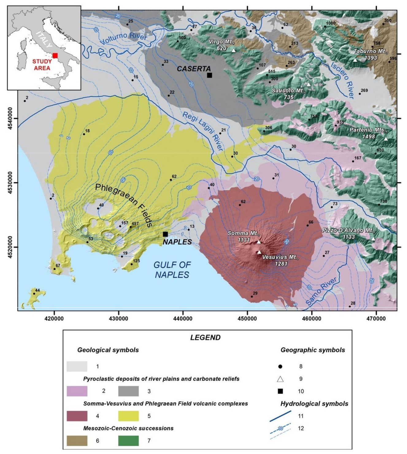
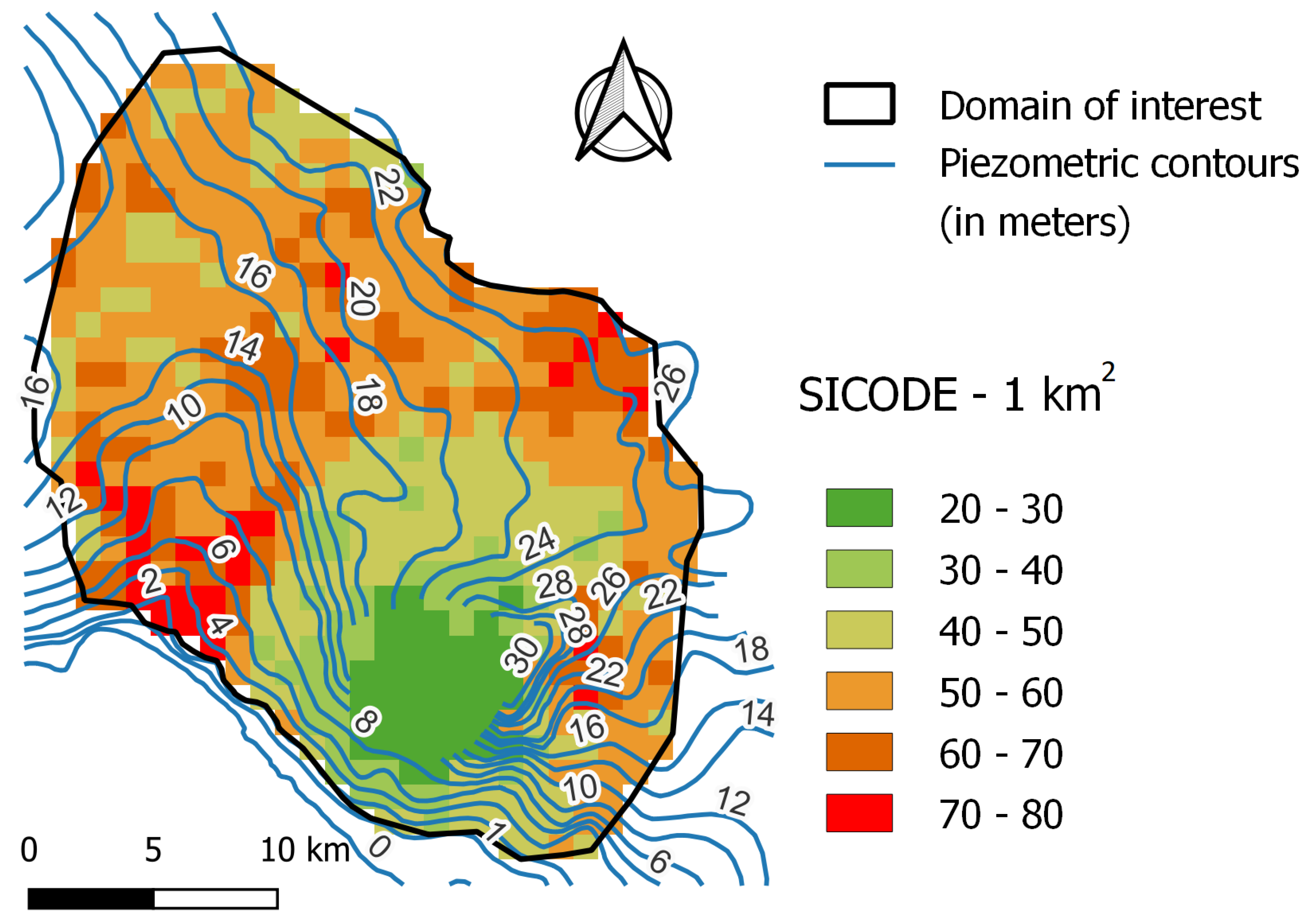
The method was applied to a groundwater catchment in the Campania region, Southern Italy, employing a previously developed index (SICODE, Catani et al. [28]) as the starting point for the $\upsilon$ evaluation. The application clearly shows that the proposed vulnerability index $\upsilon$ effectively embeds the information on groundwater flow, showing concentration of vulnerability in areas where convergence of flow is observed. Thus, groundwater flow leads to the formation of “hot spots” which are more prone to potential contamination, as function of the piezometric field in the area and the drainage groundwater catchment upstream.

The proposed method is very promising and we believe that it is quite effective in assessing aquifer vulnerability in a combined vadose zone – groundwater flow system, adopting a simplified analysis which merges the widely popular overlay and index methods and a simplified, process-based groundwater component. The method is very simple and its application can be carried out by popular geomorphological tools implemented in GIS software. We remind, however, the analysis embeds a few simplifications that are needed in order to reach a simple formulation of vulnerability, as well as a reasonable estimate of the piezometric levels are a necessary prerequisite for the analysis. Furthermore, the derived vulnerability is prone to uncertainty as it derives from the combination of overlay and index methods, that employ several different parameters, many of which being uncertain to some degree, and a piezometric field, which is also often affected by uncertainty. Hence, the method can be considered as a screening tool for a preliminary analysis of vulnerability in the aquifer systems and the identification of vulnerable areas deserving a more detailed and accurate analysis.