
Decision Support System for Sustainable Exploitation of the Eocene Aquifer in the West Bank, Palestine


1
IHE Delft Institute for Water Education, 2611 AX Delft, The Netherlands
2
Center for Environmental and Geographic Information Services (CEGIS), Dhaka 1212, Bangladesh
3
Department of Civil Engineering, College of Engineering, An-Najah National University, Nablus P.O. Box 7, Palestine
4
Hydro-Engineering Consultancy (HEC), Ramallah P.O. Box 4288, Palestine
*
Author to whom correspondence should be addressed.
Water 2023, 15(2), 365; https://doi.org/10.3390/w15020365
Submission received: 14 November 2022
/
Revised: 11 January 2023
/
Accepted: 13 January 2023
/
Published: 16 January 2023
(This article belongs to the Special Issue Groundwater Management in a Changing World: Challenges and Endeavors)
Abstract
:Groundwater is a crucial resource for water supply and irrigation in many parts of the world, especially in the Middle East. The Eocene aquifer, located in the northern part of the West Bank, Palestine, is threatened by unsustainable groundwater abstractions and on-ground pollution. Analysis and management of this aquifer are challenging because of limited data availability. This research contributes to the long-term sustainability of the aquifer by model-based design of future abstraction strategies considered within an uncertainty analysis framework. The methodology employed started with development of a single-layer steady-state MODFLOW groundwater model of the area, followed by uncertainty analysis of model parameters using Monte Carlo simulations. The same model was afterwards coupled with a Successive Linear Programming (SLP) optimization algorithm, implemented in the Groundwater Management tool (GWM) of the United States Geological Survey (USGS). The purpose of optimization was deriving five optimal abstraction strategies, each aiming to maximize groundwater abstraction, subject to different constraints regarding groundwater depletion. Given the uncertainty of model parameters, the sensitivity and reliability of these optimal strategies were then tested. Sensitivity was checked for two optimal strategies by performing re-optimization with different values of uncertain model parameters (one at a time). Reliability of the five strategies was tested by analyzing the extent of constraints’ violation for each strategy when varying the uncertain parameters using Monte Carlo simulations. Finally, the model was used for determining capture zones of wells for the five optimal abstraction strategies, land-use in these capture zones, and the associated estimates of on-ground nitrogen loading. The developed strategies were then deployed in a web-based decision support application (named Groundwater Decision Support System—GDSS), together with other relevant information. Users can analyze results of different optimal strategies in terms of groundwater level variations and total water balance results, and test consequences of uncertain parameters. Capture zones of wells for different abstraction strategies, together with land-use and on-ground nitrogen loading in these capture zones, are also presented. Results show that critical uncertain parameters are recharge, hydraulic conductivity, and conductance at key boundary condition locations. Optimal abstraction strategies results indicate that an increase in total abstractions could be between 5% and 20% from the current level (estimated at about 56 × 106 m3/year, which is about 74% of estimated annual recharge). The uncertain parameters, however, are impacting the sensitivity and the reliability of the optimal strategies to variable degrees. Recharge and hydraulic conductivity are the most critical uncertain parameters regarding sensitivity of the optimal strategies, while reliability is also impacted by the level of abstraction proposed in a given strategy (number, locations, and abstraction rates of new wells). The main novelty and contribution of this research is in combining modelling, uncertainty analysis, and optimization techniques in a comprehensive decision support system for the area of the Eocene aquifer, characterized with limited data availability.
1. Introduction
Groundwater is a crucial resource in most arid and semi-arid areas of the world. The region of the Middle East is a typical example, where countries depend heavily on groundwater resources. In the West Bank, Palestine, about 90% of the water supply is provided from groundwater [1], mainly from the so-called ‘Mountain aquifer system’ that covers most of its territory. The same aquifer system provides additional groundwater for irrigation in support of agriculture, which puts further stress on the available groundwater resources. An important aquifer in the Mountain aquifer system is the Eocene aquifer, located in the northern part of the West Bank, which provides resources for the water supply and irrigation to about 200,000 inhabitants. Overall water resources conditions in the area have many challenges [2,3,4], including: population growth (leading to increasing water demands), groundwater availability (including limitations due to constraints imposed by Israel), poor water supply infrastructure with significant water losses (high non-revenue water), and groundwater pollution (especially with nitrogen, due to untreated wastewater and poor agricultural practices). Over the last couple of decades, these challenges have led to a continuous increase of groundwater abstractions from this aquifer, resulting in a drop in groundwater levels, dried-up wells and springs, and groundwater quality problems, including nitrate pollution. Sustainable strategies for groundwater use from this aquifer are urgently needed. At the same time, the design, development, and implementation of such strategies are hampered by limited data availability, data quality issues, and a lack of groundwater monitoring systems that could provide continuous data over longer time periods.
The aim of this article is to use the case study of the Eocene aquifer, which has limited data availability, to demonstrate how methods of groundwater modelling, optimization, and uncertainty analysis can be combined to provide useful information for decision support in future aquifer management. As the main contribution of this work is in combination of these different methods, we briefly present a literature review for each, to the extent relevant for the present study.
In general, groundwater modelling has already been established as a standard method for aquifer analysis and management [5,6,7]. Most used are numerical models, among which, a de facto standard model is MODFLOW, developed by USGS [8,9]. Researchers have also attempted to develop better understanding of the Eocene aquifer area using groundwater modelling, even with limited data [10,11,12]. Given the uncertain data regarding groundwater resources in the area, coming from different sources, these modelling efforts have provided somewhat different results and conclusions. For example, different estimates for groundwater recharge from infiltrated precipitation have been used, varying in the range of 65 to 142 Mm3 per year (for the period 1991–2000) [10], with annual average recharge estimated at 72.27 Mm3 in [11], and only 23.25 Mm3 for the year 2020 estimated in [13]. Similarly, estimates of current groundwater abstractions have been highly uncertain, as well as parametrizations of the aquifer system (e.g., values of hydraulic conductivity, aquifer thickness, etc.) In these conditions, model-based analyses for determining future abstraction strategies need to be associated with more informative uncertainty analyses.
Uncertainty in groundwater models originates from different sources, such as conceptual model uncertainty (sometimes called ‘model structure’ uncertainty), uncertainty of model parameters, uncertainty in observational data, and as a consequence, predictive model uncertainty [14,15]. Different methods have been proposed for uncertainty assessment, depending on the type of uncertainty. Multi-model approaches have been proposed for conceptual model uncertainty [16], while for parameter uncertainty, the most commonly applied are probabilistic methods, often based on random sampling of parameters and simulations (using Monte Carlo techniques or similar variations) [17,18]. The objectives of uncertainty assessment also need to be considered, as they may influence the type of assessment. As presented in [19], among such objectives may be those of identifying uncertain factors that have the greatest influence on the model predictions and providing quantitative estimates of uncertainty to other users. We have not identified any prior research that considers uncertainty in groundwater modelling of the Eocene aquifer.
Regarding development of optimal groundwater strategies, research carried out over the last couple of decades has proposed a broad spectrum of approaches based on coupling groundwater simulation models with optimization algorithms [20]. Different methods have been used, that can be broadly classified in two categories: (1) response matrix approaches, in which simulation models are combined with linear, non-linear, and mixed-integer optimization algorithms [21,22], and (2) direct coupling of simulation models with global optimization algorithms (e.g., genetic algorithms), which has gained popularity in recent years [23,24,25,26,27,28]. For the case of the Eocene aquifer, only one study has been identified that used this approach to propose optimal abstraction strategies, considering sustainability concerns [29], in which a steady-state, single-layer MODFLOW groundwater model was coupled with the GWM tool of USGS [30]. Annual average well abstraction from the Eocene aquifer was estimated as 18.2 Mm3 (11.7 from Israeli wells and 6.5 from Palestinian wells) during the period from 1977 to 2003. This study considered the registered wells only, and abstractions from non-registered wells were not taken into consideration. The strategies were developed with the optimization objective of maximizing abstraction from the aquifer subject to the head constraints and groundwater withdrawal constraints. The head constraints were selected as 50% of the pre-development saturated thickness of the aquifer for the whole model domain. In addition, the second type of head constraints was set at the cells containing pumping wells as 15% of the saturated aquifer thickness to prevent dewatering. From the optimization model, it was found that an additional 23 Mm3 of groundwater can be abstracted annually from the aquifer if the pumping from the Israeli wells remains unchanged. However, such increased abstractions would lead to spring yield and lateral flow decreasing by 50% and 30%, respectively.
When considering model-based groundwater optimization for designing future management strategies, the uncertainty analyses mentioned in relation to groundwater modelling are also relevant. The identified uncertainties in the model propagate to the designed management strategies and their uncertainty needs to be assessed when they are considered for implementation. Uncertainties of the model can be directly considered in the optimization process [31,32,33], where the main challenge is reduction of computational demand (see, more recently, [34]), or uncertainty can be assessed posteriori after optimal strategies have been determined using a deterministic model [35], an approach which may require re-optimization trials. This research uses the latter approach, as will be demonstrated in the subsequent sections.
Regarding assessment of groundwater quality, analyses in the Eocene aquifer have been less available. There are no reported studies regarding groundwater quality modelling in this area. A recent analysis regarding on-terrain nitrogen loading [36] can serve as the first information base for assessing future groundwater abstraction strategies by relating areas threatened by significant pollution to the capture zones of the existing and proposed well fields (i.e., avoiding/excluding such areas from capture zones).
This research presents a model-based Groundwater Decision Support System (GDSS), in which modelling, optimization, and uncertainty analysis have been combined in an integrated framework, so that a set of groundwater abstraction strategies is proposed and presented in a web-based application. Such web applications have already been proposed in broader water resources management [37,38], including some for managing groundwater systems [39,40,41]. Their aim is primarily for supporting decision makers and stakeholders in comparing different management options and strategies, together with their consequences, as they are being considered for implementation.
Subsequent sections of this article present details regarding all GDSS research and development steps.
2. Materials and Methods
2.1. Methodological Framework
The steps in the methodological framework are presented in Figure 1.
An earlier developed MODFLOW groundwater model of the Eocene aquifer has served as initial tool for the development of GDSS (step 1). The model was developed using the GMS software of Aquaveotm [42]. This model uses estimates of total groundwater abstraction, including unregistered wells, using data on agricultural water consumption for the year 2015–2016, and distributing the associated abstraction well to the most likely (closest) irrigation areas. For this reason, the uncertainty analysis in step 2 of the methodology also included distribution of abstraction wells within well field areas as an uncertain ‘parameter’, next to the key parameters of aquifer recharge, hydraulic conductivity, and hydraulic conductance at key boundary locations. Monte Carlo simulations were used for this uncertainty analysis. In step 3, a coupled simulation/optimization model was developed using the GWM tool to design several future abstraction strategies. The optimization setup was with the objective of maximizing total abstraction, subject to some pre-defined sustainability constraints, of which the most important were those defined in terms of limits to groundwater head depletion. In step 4, these optimal strategies have then been tested for their sensitivity due to uncertain parameters (assessed in step 2). For this purpose, re-optimization was performed for two of the five abstraction strategies, with varying values of key uncertain parameters in certain range. Reliability analysis of step 5 was performed by defining reliability in terms of percentage of locations (model cells) where the specified constraints would not be violated, as uncertain parameters were varied within Monte Carlo sampling and simulations. (Note that this step does not include re-optimization as the one performed in step 4). For assessing the potential of groundwater nitrate pollution associated with the identified strategies (step 6), the simulation model was first used to determine the capture zones of the existing well fields (as defined in the strategies). These were then overlaid with land-use data and on-ground nitrogen loading data, to have the first impression about the pollution potential. All previous steps led to the final step 7–GDSS setup as a web-based application containing both groundwater quantity and quality information. Following the presentation of the Eocene aquifer study area in Section 2.2, details of all methodological steps are presented in subsequent sections.
2.2. Study Area
The Eocene aquifer is located in the north-eastern part of the West Bank, Palestine, as depicted in Figure 2. It covers the districts of Jenin, and parts of Nablus and Tubas. The total area of the aquifer is about 640 km2 and 429 km2 lies inside the West Bank. The elevation of the Eocene aquifer varies from 15 to 950 m above sea level (masl), also shown in Figure 2. The southern part of the aquifer is mostly hilly while the north-western part has a flat terrain. The topography in the central and north-eastern parts ranges from moderately flat to hilly. The aquifer serves as the main water supply source for the area. Several springs have been developed from the aquifer, especially in the hilly terrain. Water from springs and pumping wells is utilized for irrigation and water supply purposes.
The Eocene aquifer area has a Mediterranean climate with two seasons: a wet winter and dry summer. Rainy season spreads from October to May and the highest rainfall occurs during January. The annual average rainfall during the period of 1952 to 1999 (from eight rainfall stations located inside the Eocene aquifer area) is about 510 mm with variations from 400 to 630 mm. The south-western part of the aquifer receives higher rainfall, while the rest of the aquifer area has a very small variation of rainfall. The Eocene aquifer area has a minimum temperature of about 7 °C during the winter, and a maximum temperature of about 33 °C during the summer.
The geological formations in the area form two aquifers: deep and shallow. The deep aquifer (not the subject of this study) is formed in limestone, dolomite, and marl from Turonian and Cenomainian ages of the late Cretaceous [10]. The upper aquifer is formed in limestone, chalk, and chert from the Eocene, with some Quaternary alluvial zones. There is a transition zone of chalk in between the two aquifers. The Eocene aquifer that is the subject of this study is the upper, unconfined aquifer, which has thickness varying between 200 m and 680 m.
Key conditions that influence aquifer recharge from infiltrated precipitation are soil types and land use in the area. The main soil types are Terra Rossa, Mediterranean Brown Forest Soils, Alluvial Soils, Colluvial–Alluvial Soils and Brown Alluvial Soils covering 49%, 16%, 14%, 13%, and 8% of the study area, respectively [36]. The soils are quite fertile and significant agricultural activities have developed, especially in the lowland areas in the middle and the north of the area. Land use is mainly consisting of agriculture (crops and trees, 37%), shrub land (40%), urban areas (7%) and the forests (16%). The spatial distribution of these land use categories is given in Figure 3. (Note that a more detailed land use map has been used in the GDSS, as will be shown in Section 3).
As mentioned earlier, an important aspect with quite large uncertainty is the total abstraction of groundwater from the area. This research used available records from the Palestinian Water Authority (PWA) at the time, with 129 registered (licensed) wells over the Palestine part of the aquifer with a total capacity of 4.24 Mm3/year. Among them, 45 wells are used for agriculture (pumping: 2.84 Mm3/year), 5 wells for domestic water supply (0.97 Mm3/year), and 4 wells for both agriculture and domestic water supply (0.43 Mm3/year). A number of wells that have been used in the past have dried up and/or have been abandoned. The distribution of registered wells is presented in Figure 4. As mentioned earlier, it is estimated that the total abstraction from the aquifer is much larger, due to unregistered wells.
It should also be noted that the Eocene aquifer area used to have a number of springs prior to the development stage, with a total discharge of about 22.1 Mm3/year (estimated from historical data), but many of these springs have dried up and the annual discharge from springs has been significantly reduced.
2.3. Available Groundwater Flow Model and Additional Data
2.3.1. MODFLOW Model of the Eocene Aquifer
The MODFLOW model has been developed and calibrated by the Hydro-Engineering Consultancy (HEC) prior to this research. It is a steady-state model with a single unconfined layer (thickness, 200–680 m), covering an area of 540 km2 discretized with 349 rows and 234 columns, using local grid refinement at the locations of well fields. The model has 62,996 active cells with cell size varying from 10 to 100 m in the x-direction and 10 to 250 m in the y-direction.
The boundary conditions of the model were set up as mostly impermeable, with a general head boundary introduced at the northern side, and several drain boundaries at the eastern side to represent the spring zones. The location and distribution of unregistered wells were approximated based on the quantity and distribution of irrigated lands, and their pumping rates were estimated based on the agricultural water consumption per unit area, and irrigated areas from the year 2015–2016. This resulted in a total of 195 wells, including 9 wells from the Israeli part of the aquifer. The abstraction rate of the wells varies from 50 to 2000 m3/day. The distribution of wells and the boundary conditions are presented in Figure 5.
The model used spatially distributed recharge and hydraulic conductivity. Recharge was estimated using empirical formulas that calculate recharge rates as a percentage of precipitation rates (from multiple stations), following the methodology that uses variation of groundwater levels and its relation to inflows and outflows, described in [43]. Hydraulic conductivity was estimated based on available geological maps and cross sections of the area. The model was calibrated against data from 14 observation wells for the steady state condition. Aquifer hydraulic conductivity, aquifer recharge, and hydraulic conductance of the drain and general head boundary were considered as calibration parameters. The final aquifer recharge and hydraulic conductivity distributions are shown in Figure 6, together with the performance of model calibration.
As mentioned earlier, this model uses the GMS software of Aquaveotm. For uncertainty analysis, optimization, and particle tracking analyses carried out in the next steps of this study, it was converted into the native MODFLOW-2000 format. The python floPy library [44] was used to simulate and extract data from this model format.
2.3.2. Additional Data Used for GDSS
Next to the MODFLOW model described in the previous section, which was the main tool for this research, some additional data were used, particularly for the groundwater quality part of the GDSS. First, a more detailed land use map was used (compared to the one shown in Figure 2), with 17 different land use classes. Secondly, using the research results from the identification of nitrogen pollution sources in the Eocene aquifer reported in [36], a map of on-ground total nitrogen loading has been prepared. This map was then used in the analysis of the potential nitrogen pollution in the area, and, particularly in the capture zones of the existing well fields as defined in the optimal pumping strategies.
2.4. Uncertainty Assessment
2.4.1. Identification of Uncertain Parameters
Recharge to the Eocene aquifer from infiltrated precipitation and hydraulic conductivity are the most important parameters to be considered in uncertainty analysis, due to their influence on overall groundwater flow conditions. Next to these two, hydraulic conductance of the drain and general head boundary was also considered uncertain, as well as well distribution within identified well fields. The approach taken for assessing the bounds for uncertainty analysis for each of these four parameters is described as follows:
(a) Recharge
Using precipitation records for the period 2008–2018 for 13 stations, annual recharge values have been calculated using the same empirical formulas, described in [43]. From this analysis, it was concluded that annual recharge for most stations follows nearly normal distribution. The mean and standard deviation for all stations is given in Figure 7.
With these results, it was decided to use sampling from normal distribution in the subsequent uncertainty analysis of the recharge. For each station, the mean and standard deviations were used to fit such distribution. The sampling was carried out in the range of mean ± standard deviation, and the generated recharge was applied to the model cells located inside the influence zone of each station as indicated in Figure 6a.
(b) Hydraulic conductivity
As there were no additional data regarding hydraulic conductivity, the value obtained during model calibration was used as a reference value, and uniform sampling in the range −25% to +25% from that reference value was used for uncertainty analysis. Similarly to the recharge, the values were assigned to cells within each hydraulic conductivity zone.
(c) Hydraulic conductance (drains and general head boundary)
As for hydraulic conductivity, the values obtained during calibration were used as a reference, and sampling in the range −25% to +25% was used in the uncertainty analysis.
(d) Wells distribution within well fields
The wells located in the Palestinian part of the aquifer were grouped into 17 well fields. They included both registered and unregistered wells. The extent of each well field was delineated based on agricultural land surrounding the wells using on-screen digitization in Google Earthtm. Then, each well was randomly assigned to one modelling cell located inside the corresponding well field during uncertainty analysis. Figure 8 shows two examples of well field delineation (a and b), and possible locations of wells inside any of the well fields identified (c). The location of Israeli wells was considered fixed during this uncertainty assessment.
2.4.2. Experimental Setup for Uncertainty Analysis
Groundwater heads were primary uncertain model outputs to be assessed given the uncertainty of the identified parameters presented in previous section. For this purpose, Monte Carlo Simulations (MCS) were executed using a Python script that performed the following: generation of random variables for all uncertain parameters (based on the defined range and statistical distribution), updating the corresponding MODFLOW model files, simulating MODFLOW, extracting the results and performing necessary computations. The floPy library was utilized for MODFLOW model run and for extracting results. A flow chart for all the steps of the uncertainty analysis is presented in Figure 9. (Uncertainty was analyzed for each parameter separately, as well as combined uncertainty from all parameters). The model was simulated for the following predefined sample sizes (N): 25, 50, 100, 150, 200, 250, 300, 350, 400, 450, 500. The groundwater head at every modelling cell and the outflows from the aquifer were stored for every realization in order to estimate statistics.
Standard error (SE) of mean and standard deviation of groundwater head was estimated at selected locations for each predefined sample size to evaluate the convergence of MCSs. SE was estimated using the Central Limit Theorem for the mean and Bootstrap standard error for the standard deviation. In total, 23 locations were selected over the aquifer area for performance assessment of MCS, as shown in Figure 10.
2.5. Development of Abstraction Strategies Using Model-Based Optimization
2.5.1. Identification of Abstraction Strategies Based on Aquifer Saturated Thickness
For sustainable exploitation of the Eocene aquifer, a key condition is preserving the saturated thickness of the aquifer (avoiding groundwater depletion), while still attempting to maximize abstractions. Depletion of saturated thickness might lead to a decrease in aquifer storage, pumping rates of wells, increased cost of installing and operating pumping wells, compaction of the aquifer, and overall, decrease the aquifer sustainability. All identified strategies in this study have been defined in relation to Pre-development Saturated Thickness (PST), which represent saturated thickness without any abstraction. Representation of the strategies considered is depicted in Figure 11, which presents a conceptual cross-section through the aquifer, with the x-axis representing a conceptual horizontal dimension, and the y-axis representing saturated thickness in percentages, with PST = 100%.
As can be seen in Figure 10, five strategies have been defined, as follows:
Strategy 01: Allow groundwater level depletion up to 60% of PST for areas where the groundwater level is above 60% of PST. For the remaining areas, maintain the existing groundwater level.
Strategies 02, 03, and 04: The concept of strategies 2, 3, and 4 is the same as that of strategy 01, but that allowed depletions are up to 50, 40, and 30% of PST for areas where the groundwater level is above 50, 40, and 30% of PST for strategy 02, 03, and 04, respectively. Maintain the existing groundwater level for the remaining areas.
Strategy 05: This is a restoration (conservative) strategy. Restore the groundwater level up to the limit of 30% of PST for areas where the existing groundwater level is below 30% PST. For the remaining areas, maintain the existing groundwater level.
These strategies are, in fact, used for setting the head constraint in the optimization formulation described in the following section.
2.5.2. Optimization Formulation
The optimization problem to be solved has been formulated as follows:
Decision variables:
The pumping rates and locations of wells (existing and potentially new) are chosen as decision variables. A well for which the pumping rate will be varied during optimization is called a managed well. There are also non-managed wells (e.g., Israeli wells) for which pumping rates are fixed during the entire simulation period. In addition to the 186 existing wells, 172 potential wells were also considered as managed wells, as shown in Figure 12. The areas which have an aquifer thickness greater than the 50% of PST and have agricultural land use were considered for a potential well location. The agricultural areas were identified using the land use map and Google Earth satellite image.
Objective function:
The objective function of optimization was to maximize the weighted sum of pumping rates from the aquifer. Mathematically, it can be expressed as:
where is the sum of the weighted groundwater pumping rates, N is the number of managed wells, is the pumping rate from managed well i, and is the weight associated with pumping rate for managed well i. A weight of 1.0 is used for wells located in the existing well field, and a weight of 0.8 is used for potential well fields. As there is existing infrastructure for water abstraction and water use in the existing well fields, higher weight is given to those locations. The weight of 0.8 for potential well fields was a reasonable assumption, so that such well fields would be still considered by the optimization algorithm (and not avoided if the weight would be lower, e.g., 0.4–0.5), but not favored as much as the existing well fields.
Constraints:
Three different types of constraints were used in the optimization, as follows:
Hydraulic head constraints:
Head constraints were specified to limit the depletion of the groundwater head beyond specified limits. The head constraints can be expressed mathematically as:
where = is the specified lower limit on head at locations i, j, k. The head constraints were specified based on the developed pumping strategies described in Section 2.4.1 and applied at 205 control locations (Figure 11). The control locations were uniformly distributed over the model domain with a distance of around 1500 m in both directions.
Groundwater withdrawal constraints:
These are lower and upper bounds of pumping rates at individual wells (decision variables):
Lower bounds of the decision variables were set at zero, as this is mandatory for GWM while using linear and successive linear optimization [30]. The upper bound was specified at 125% of the current pumping rate for the existing wells, to allow more pumping to meet future demand. For all new potential wells, the upper bound was set at 800 m3/day.
Linear summation constraints:
Linear summation constraints for the decision variables were introduced to ensure a minimum quantity of water to meet the current demand for each existing well field. In addition, an upper limit of the total pumping quantity was also set to avoid over abstraction of water at any particular location. Such constraints have been defined as:
where and are the minimum and maximum water demand, respectively, for a well field, p is the total number of wells in a well field, and is the optimal pumping rate for flow rate decision variable p. For each existing well field, the lower and upper bound were set at 80 and 120% of the existing pumping quantity, respectively.
This optimization problem was solved using the GWM tool, resulting in five optimal abstraction strategies. Linear Programming (LP) and Successive Linear Programming (SLP) (non-linear) optimization were carried out using the response matrix approach [30]. As the Eocene aquifer is an unconfined aquifer, characterized with non-linear responses, better results were obtained using SLP, which will be reported later in Section 3.
2.6. Sensitivity and Reliability of the Optimal Abstraction Strategies
For strategies 02 and 03, sensitivity analysis of the optimal abstraction was performed due to uncertain aquifer recharge, hydraulic conductivity, and hydraulic conductance, to reveal the influence of these parameters on the optimal solutions. The sensitivity analysis, in fact, involved re-optimization. This analysis is intended to show how the optimal solutions for the defined strategies would change if uncertainty of the parameters is considered. Each parameter was changed with a certain percentage, one at a time, and the optimization was repeated using the formulation described in Section 2.5. The following steps were followed:
- Change the hydraulic conductivity, hydraulic conductance, and recharge by a certain percentage (−20%, −10%, 0%, +10%, and +20%), one parameter at a time.
- Perform optimization for five different pumping strategies.
- Compare the objective function values of the optimal solutions for different parameters and different pumping strategies.
The developed optimal strategies were also tested in terms of reliability, given the uncertainty of the identified parameters. Without any re-optimization, Monte Carlo simulations were performed on the original optimal model (for each of the five strategies) considering the uncertain aquifer recharge, hydraulic conductivity, and hydraulic conductance of drains and general head boundary. The fulfilment of hydraulic head constraints was assessed for every realization of Monte Carlo simulation and considered as a success or failure for that realization. Locations of pumping wells were excluded from this analysis. The range and statistical distribution of uncertain parameters were the same as those used during uncertainty analysis of the base model (Section 2.4.1). Based on the success and the total number of simulations, reliability was estimated at every modelling cell for the given optimal pumping strategy using the following equation [35]:
where R is the reliability (in percentage), F is the number of failures, and N is the total number of simulations.
2.7. Assessing Nitrogen Pollution Potential for the Optimal Abstraction Strategies
To obtain initial assessment of pollution potential for the developed optimal abstraction strategies, backward particle tracking was performed to determine the capture zones of the existing wells, as proposed in each of the five strategies. The MODPATH particle tracking tool [45] was used for this purpose, using the groundwater flow results from the MODFLOW model. Such capture zones were determined for two periods of assumed abstraction: 20 years and 100 years. These capture zones were then converted to shape files, so that they can be deployed on the GDSS and overlaid together with land use data and data regarding on-ground nitrogen loading. This approach enables more detailed analysis of pollution potential for the areas belonging to the capture zones, which could contribute to better design of existing wells’ protection zones and pollution control. The results of this analysis are presented in Section 3.4, where GDSS outputs are presented.
2.8. Groundwater Decision Support System (GDSS) Design and Implementation
GDSS was set up as a web application with the goal of enabling better access to the results of this research to different stakeholders. The design of its groundwater quantity component was oriented to analyzing results from the developed optimal abstraction strategies, primarily, groundwater head distributions (and differences compared to existing conditions), and overall water balance results. Additional functionalities were also included in the design, such as running the MODFLOW model with different wells distribution and with variations of aquifer recharge and hydraulic conductivity values. In the groundwater quality component, the capture zones of wells for the different strategies are presented together with their overlays with land use and on-ground nitrogen loading data.
Standard client and server programming technologies were used for GDSS implementation, as depicted in Figure 13.
Main web pages of the application are served by the Apache web server. The maps embedded within the web pages receive spatial data from GeoServer. Most of these spatial data are stored in a Postgres database, with few static layers stored as shape files. Main communication with the servers is via Jquery, and Pyhton scripts are used for execution of the MODFLOW model or update of the Postgres database (e.g., update wells data).
Key functionalities of GDSS can be summarized as follows:
- Select and load optimal strategies (pumping wells, together with associated information) and visualize results as spatial data (groundwater heads) and water balance.
- Modify selected strategy (add, edit, or delete wells; change recharge or hydraulic conductivity), run the MODFLOW model, and present the modified results.
- Visualize well capture zones of the optimal strategies together with land use or on-ground nitrogen loading data.
3. Results
3.1. Model Results for Exiting Conditions
Figure 14 presents the simulated groundwater head distribution and the water balance results. Saturated thickness of the aquifer, as percentage of PST (which varies between 10 and 650 m in absolute values), is given in Figure 15.
As shown in Figure 14, the groundwater head of the aquifer varies from 10 to 375 m above mean sea level. It is highest in the southern part of the aquifer, and lowest in the northern part. Thus, the general direction of the head gradient (and of groundwater flow) is from south to north. From the middle part of the aquifer to the north, the head gradient is relatively steeper compared to the southern part, corresponding to the change in hydraulic conductivity, as shown in Figure 6b. The water balance results indicate that out of the total inflow of 75.6 Mm3 per year, provided by recharge from infiltrated precipitation, 74% is pumped out via wells, 24% flows out via drains (representing springs), and the remaining 2% flows out as groundwater flow downstream via the northern general head boundary.
Figure 15 shows clearly that most of the current abstractions are located in the middle of the aquifer, especially in the mid-western zone, where the saturated thickness is already at only 20 to 30% of PST. Limitation of abstraction, or even groundwater restoration, would be needed for these zones. Opportunities for further groundwater resources development may be more in the south and especially, in the north of the Eocene aquifer.
3.2. Uncertainty Assessment Results
3.2.1. Convergence of Monte Carlo Simulations (MCSs) for Uncertainty Analysis
The convergence of MCSs was evaluated in terms of standard error (SE) of mean and standard deviation of simulated groundwater head at 23 locations indicated in Figure 10. Results for SE of the mean for the different predefined sample sizes are presented in Figure 16. Standard deviation SE results followed a similar pattern. SE rapidly diminishes till about 200 simulations and then becomes more or less stable. The errors of mean and standard deviation were 0.4–1.2 m and 0.5–0.75 m, respectively, after 500 simulations. Higher errors were registered for locations 10, 11, 12, and 16, located in a zone with a high range of uncertainty, as shown in the next section. The obtained results indicate that the sample size of 500 simulations is sufficient for further uncertainty analysis.
3.2.2. Results from Uncertainty Analysis of Identified Parameters
First, the uncertainty analysis was carried out for each uncertain parameter individually (aquifer recharge, hydraulic conductivity, well location, and hydraulic conductance). The obtained fluctuations of the groundwater head are shown in Figure 17a–d.
The highest uncertainty is obtained for aquifer recharge, especially in the mid-western part of the aquifer, where maximum fluctuation was found to be as high as 175 m. This area has a high density of wells and low hydraulic conductivity, so a small decrease in recharge results in a high depletion of groundwater. The uncertainty of groundwater level due to hydraulic conductivity is more or less uniformly distributed, with a range of 30–50 m in the south and of 10–30 m in the north. Regarding the spatial distribution of wells, the distribution of uncertainty follows the pattern of the distribution of well fields. It is higher in the mid-western and south-eastern parts (with high wells density), where maximum fluctuation was found to be 100 m. The hydraulic conductance has a very small influence on model uncertainty, mainly limited to zones adjacent to the model boundaries. Only the zone of the south-eastern drain boundary has a relatively higher uncertainty of 30–50 m.
Secondly, combined parameter uncertainty was assessed, and the results in terms of groundwater head fluctuations are presented in Figure 18. The fluctuation ranges from 0 to 200 m, with a spatial pattern of uncertainty similar to the one due to aquifer recharge—the parameter that brings the highest model uncertainty. In the north, the uncertainty is lower, with a fluctuation range of 0 to 75 m. In the mid-western part (locations 10, 11, 12, 16), it is highest. Another highly uncertain zone is the south-eastern part of the aquifer, influenced by the uncertainty induced by the well location and hydraulic conductance.
3.3. Optimal Abstraction Strategies Results
3.3.1. Wells Distribution and Water Balance Results for the Five Optimal Strategies
Table 1 shows summary water balance results for the five optimal strategies in terms of optimized total abstraction compared to the existing conditions (only Palestinian wells).
Figure 20, Figure 21, Figure 22, Figure 23 and Figure 24 show the wells distribution for the five strategies, and Figure 25 shows the groundwater level change compared to present conditions for all five strategies.
Figure 20, Figure 21, Figure 22, Figure 23 and Figure 24 indicate that three potential well field areas were identified from the distribution of optimal pumping locations. The first one is in the north-western region. It has the highest potential for groundwater abstraction under all strategies. The second is one located in the south-eastern region and the last one at the mid-eastern region of the aquifer. These areas have higher pre-developed aquifer thickness compared to their surrounding areas. From the existing wells, around 25% were resulting in a zero pumping rate after optimization, while the remaining 75% were set at their upper limit of the groundwater withdrawal constraint, with very few exceptions. Despite 25% of wells having zero pumping after optimization, the locations of optimal pumping wells were more or less evenly distributed over the existing well field areas.
Figure 20, Figure 21, Figure 22, Figure 23 and Figure 24 also show that, as expected, the optimal strategies propose that most new wells are located in the north and south, with the largest number of such wells being proposed for Strategy 04, which allows for the largest groundwater depletion, and has the highest total abstraction rate. Strategy 05 has only a small increase in total abstraction compared to existing conditions (1.4%), because it is a restoration strategy. This strategy proposes the re-distribution of pumping over larger areas, rather than concentration in the mid-western zone, as in current conditions.
Finally, Figure 25 presents the changes of groundwater levels for the five strategies compared to the present conditions (presented in Figure 14). The results show clearly the progressive drop of groundwater levels (and consequently, aquifer saturated thickness) for strategies 01–04, and the increase of groundwater levels for the restoration strategy 05.
3.3.2. Sensitivity and Reliability of the Five Identified Optimal Abstraction Strategies
The sensitivity of the optimal abstraction rate due to change in uncertain aquifer recharge, hydraulic conductivity, and hydraulic conductance was estimated and shown in Figure 26 for strategy 02 (results for strategy 03 are very similar). The optimal abstraction rate is most sensitive to recharge, followed by hydraulic conductivity and hydraulic conductance, which is the same sequence as in the uncertainty analysis. Total optimal abstraction rate increased about 7.5 to 7.8 Mm3/year for a 10% increase in recharge. For each 10% increase in hydraulic conductivity, the optimal pumping was reduced by 2.7 to 3.5 Mm3/year. The sensitivity of optimal abstraction due to hydraulic conductance is less than 0.5 Mm3/year for each 10% charge in hydraulic conductance of model boundaries.
A summary of the reliability of the five optimal strategies due to uncertain parameters is provided in Figure 27.
As expected, reliability is closely correlated with the abstraction from the aquifer. It decreases as the total abstraction increases. For strategy 01, the middle portion of the aquifer is less reliable (40–60%) due to the high abstraction from that region, where reliability for the rest of the area is above 50%. There is an uncertain zone introduced in the north-eastern part of the aquifer due to the new potential well field adjacent to it, and low aquifer thickness at that location. The less reliable areas expand for strategy 02, and even more for strategy 03, where the middle part of the aquifer becomes 20 to 40% reliable and the reliability of the mid-western part is as low as 20%. Strategy 04 is the worst in terms of reliability, with values below 10% in the north-western part due to high abstraction from the new well field from that area. In contrast, the reliability is increased in the mid-eastern region (compared to strategy 03) due to the decrease in pumping rate of nearby well fields. Strategy 05 performs best in terms of reliability as it is a restoration strategy. It has reliability above 60% for most of the areas, and even above 80% in some areas.
3.4. GDSS Visualization Results
The main interface of the groundwater quantity part is presented in Figure 28. The map interface is used for showing data on wells distribution (each well’s data are editable by clicking on the respective dot), groundwater levels, or differences in groundwater levels compared to present condition, when a certain optimal strategy is selected. The bottom part of the interface is used for selecting a particular strategy, modification of aquifer recharge and/or hydraulic conductivity (uniformly by ±25%), and reporting of the overall water balance result after a particular model run. The ‘Simulate’ button on the right executes the MODFLOW model run, after which the new results are made available. Note that the user can run the five pre-defined optimal strategies and view their results, but also can modify them by introducing different recharge, hydraulic conductivity, or pumping wells inputs, run the model, and see results of such a modified strategy.
Figure 29 shows the results after selecting a different strategy (Strategy 03) and viewing results in terms of differences of groundwater head compared to present conditions.
In the groundwater quality component, the first interface shows wells capture zones per well field and for selected strategies. Figure 30 shows results for current conditions and for strategy 03.
Next, the user interface shows the overlay of the different capture zones with land use data, as shown in Figure 31 (example of strategy 5). Clicking inside each land use unit within a particular capture zone presents further information below the map interface.
Similar information can be provided for capture zones and on-ground nitrogen loading, as shown in Figure 32 (example of strategy 03).
4. Discussion
This study has been performed to address important challenges in groundwater assessment and design of future exploitation strategies in cases with limited data availability, as with the Eocene aquifer area in the West Bank. However, while more data with better quality are needed, actions leading towards sustainable groundwater use should not be impeded by such issues. One approach to overcome this situation, addressed in this research, is to reveal the uncertainty in the designed and proposed solutions and strategies. Uncertainty quantification, sensitivity, and reliability analyses of the kind presented here may not necessarily lead to immediate selection of best strategies for implementation. However, they can serve as a starting point for discussion and analysis of possible realistic strategies, and they may also provide focus on needs for critical data that need to be prioritized for collection and analysis. This process can be further supported if the results of such research are presented in a decision support application such as GDSS.
Considering the presented results and the above provided context, our discussion addresses concerns specific to the situation in the Eocene aquifer.
Starting with the developed groundwater flow model, we can say that it provides reasonable representation of the groundwater conditions in the area, even though it was calibrated with limited data. The most significant novelty in this model, compared to previous ones developed for the same area, is in the usage of estimates of groundwater abstraction for irrigation, based on agricultural water use. Most of the unregistered wells in the area are in fact used for irrigation purposes, and past studies have underestimated such abstractions. In the model, such abstractions have been allocated to well fields located close to irrigation fields, in a random manner, but the subsequent uncertainty analysis showed that the actual wells’ distribution within well fields does not bring significant uncertainty in the model results, at least for this regional scale model.
The model contributes to the understanding of the current situation of the Eocene aquifer in terms of water balance, groundwater levels, and flow patterns, together with the assessment of model uncertainty, as follows:
- Average annual recharge of the aquifer was estimated at 75.6 Mm3 and it is the only inflow to the system. About 74% of this inflow is abstracted through pumping wells and the rest is outflow through the drains and general head boundary downstream.
- Groundwater head of the aquifer varies from 10 to 375 m above mean sea level. The general direction of the head gradient is from south to north. The saturated aquifer thickness is in the range 20–80% of pre-developed saturated thickness (PST).
- The mid-western part of the aquifer is already overused with the current aquifer thickness below 20–30% of PST. The southern and northern part are in better conditions with potential for further utilization.
- Simulated groundwater head was the primary model output for which uncertainty of parameters was tested. Out of the four parameters considered in the uncertainty analysis (recharge, hydraulic conductivity, hydraulic conductance at the boundaries and wells distribution within well fields), aquifer recharge brings the highest uncertainty and has the most impact on modelling results, followed by hydraulic conductivity. Groundwater head variations due to overall (combined) uncertainty were found to vary in the range of 40 to 95 m between the 5th percentile and 95th percentile, while in the inter-quartile range, they varied between 20 and 40 m throughout the aquifer.
Of course, the developed groundwater flow model has a number of additional uncertainties that need to be addressed. This study was restricted to analysis of uncertainty of model parameters, with a focus on parameters that are known to have the highest impact on modelling results. The results show better assessment of groundwater recharge, using better data, and more detailed soil water balance models may be needed in future studies. Second in importance is the aquifer hydraulic conductivity, for which further data should also be collected. Future studies need to extend the uncertainty analysis to include the conceptual model uncertainty, which has not been addressed in this study. The very fact that the current model has been developed as a single-layer model is a simplification, and further analysis of different conceptual models needs to be investigated [14,16,46].
For future abstraction strategies, the developed model was combined with a Successive Linear Optimization (SLP) algorithm in GWM to derive the following results:
- Five pumping strategies were developed based on the pre-developed saturated thickness (PST) of the aquifer. Allowable depletion up to 60, 50, 40, and 30% of PST was introduced for the places where the existing groundwater level is above that level for strategy 01, 02, 03, and 04, respectively. For the rest of the areas, the existing groundwater level was maintained. For strategy 05, restoration of the groundwater level was introduced, bringing it to the level of 30% of PST where it is below 30% PST.
- The objective function of optimization for all strategies was to maximize the weighted sum of well pumping rates, subject to hydraulic head constraints at 205 locations, withdrawal constraints for each managed well and linear summation constraints for each well field.
- Total optimal pumping rate from the aquifer was obtained as 52.6, 54.1, 56.7, 60.2, and 50.1 Mm3/year for strategy 01, 02, 03, 04, and 05, respectively, considering existing and potential well locations. Three new potential well field areas were identified, located in the north-west, the south-east, and at the middle-east region of the aquifer.
Out of the five proposed sustainable strategies, the restoration strategy 05 seems best for aquifer sustainability. It redistributes the abstraction over larger areas, instead of concentrating it in the mid-western region. However, that strategy provides only a small increase of the total water available, and the newly proposed well fields are further from locations where water is needed and where there is available infrastructure for water transmission and distribution. Therefore, this strategy needs to be considered in critical comparison with one of the four other strategies (notably 02 or 03), which allow for more groundwater level decline but also provide more water and at locations where it is more needed.
In all optimal strategies, there was also a consequence of the decrease of total outflow via the drains and the general boundary in the north, with a larger decrease of such outflows as the total optimal pumping was higher, as might be expected. In this research, experiments were also performed with the introduction of additional constraints that would limit these outflows to a minimum amount, and in these cases, the total optimal abstraction was somewhat smaller. Such analyses should be also considered in future, as additional knowledge regarding minimum constraint values that should be used in these locations will become available.
Sensitivity analysis of the optimal strategies with respect to uncertain model parameters brought the following results:
- Sensitivity analysis, performed by re-optimization of strategies 02 and 03 with varying parameter values, confirmed that the optimal abstraction is most sensitive to recharge, followed by hydraulic conductivity and hydraulic conductance.
- Example results from the sensitivity analysis of strategy 02 show that the total optimal abstraction increases by 7.5 to 7.8 Mm3/year for a 10% increase in recharge. For each 10% increase in hydraulic conductivity, the total optimal abstraction reduces by 2.7 to 3.5 Mm3/year. A change in hydraulic conductance at the model boundaries of 10% results in less than 0.5 Mm3/year variation of total optimal abstraction.
One peculiar result from this analysis is that the optimal solutions result in smaller total optimal abstraction as hydraulic conductivity increases. As the optimization is run with same constraints, for higher hydraulic conductivity, groundwater flow is faster towards the drains and the general head boundary and water can easily flow out from the system. This was actually confirmed with water balance results that indicated corresponding increases of outflows for conditions of larger hydraulic conductivity and smaller total optimal abstraction. When this happens, the head constraints in locations relatively close to the boundaries are hit, leading to an optimal result with lower total abstraction. Future analysis could consider re-formulation of optimization for different hydraulic conductivity values.
Summary results from the reliability analysis indicate that:
- The reliability of the pumping decreases with an increase in the abstraction rate.
- The reliability of strategy 01 was in the range of 40 to 60%. Strategy 04 was the worst in terms of reliability, where reliability dropped below 10% in the north-western part due to high abstraction from the new well field in that region.
- Strategy 05 performed best in terms of reliability as it was a restoration strategy. It had reliability above 60% for most of the areas, with some areas having reliability above 80%.
Reliability analysis indicated that next to the identified uncertain parameters the amounts and locations of abstraction are also important. Strategy 04 had low reliability in the north, where many new abstraction wells were proposed. However, it needs to be also noted that reliability in this study is defined solely in terms of the number of locations where the proposed head constraints are met, in a ‘yes/no’ (binary) approach, when parameter uncertainty is considered. Future studies could consider a more sophisticated definition of reliability, considering, for example, the level of constraint violation.
Results from the Eocene aquifer groundwater model, the design and development of optimal abstraction strategies, and uncertainty analysis were combined and brought together in the GDSS web application. It has functionalities of visualizing map-based results of groundwater head and water balance for the five developed abstraction strategies, as well as possibilities for executing simulations with different inputs for abstraction wells, recharge, and hydraulic conductivity. In its current form, it has the potential to be informative and a support tool for PWA. A dedicated workshop with PWA for demonstrating GDSS (which was conducted online due to COVID-19 epidemic restrictions) revealed that water resources experts in that organization are particularly interested in the possibilities of analyzing different alternatives of groundwater abstraction using the provided functionality of online simulation with the MODFLOW model. While this is understandable from a water-resources planning point of view, it needs to be realized that this functionality is feasible only if the model is with short running time (a steady state model in this case). More complex simulations (e.g., transient), with longer running time, are not suitable for online deployment. Selection of most suitable alternatives and strategies and their deployment in GDSS therefore remains important, especially for future use of such a system with other stakeholders. For GDSS to become a publicly available web application that could be shared and accessed by different stakeholders, it needs to be further developed into a stable application that can be hosted and maintained in the West Bank. Furthermore, to meet the real challenge of design and implementation of sustainable strategies by involving a broader group of stakeholders and users dependent on groundwater, the application needs many additional functionalities, such as: further improvement of the groundwater flow model and the associated optimization and uncertainty analysis, better comparison of identified strategies (including potentially use of Multi-Criteria Analysis), and, perhaps most importantly, presentation of results in a form suitable for diverse stakeholders (using appropriate scale, form of presentation, language, etc.)
Finally, further research work on aspects of groundwater quality is also needed. The initial data presented in GDSS only give indications about possible critical zones where pollution protection would be most urgent. Further development of groundwater quality models (also known as fate and transport models) is needed, but such efforts need to go in parallel with improvements in the groundwater flow modelling, as the flow conditions provide a basis for contaminant fate and transport modelling. Uncertainty analyses of such groundwater quality models, similar to those presented here, should also be considered, before their potential inclusion in optimization analyses and applications like GDSS. Furthermore, the model-based optimization introduced here had the objective function and constraints related only to water quantity. If water quality is considered, the optimization problem needs to be re-defined to include at least some water quality constraints (e.g., nitrate concentrations in the pumped water from the designed wells). This would require coupling of an optimization algorithm with the more complex and highly non-linear groundwater quality model. A different optimization algorithm may be needed for this purpose, as well as modelling methods that will reduce computational costs that would be much higher.
In a broader, more generic context, beyond the current analysis of the Eocene aquifer, this research touches upon some challenging questions regarding the role of uncertainty analysis of groundwater models (and environmental models in general) in decision support. The challenging questions are in fact related to the contribution of uncertainty analysis to sound decision making, especially when the models involved have significant uncertainty in their structure and/or parameters. The presented research in the Eocene aquifer confirms that uncertainty analysis of groundwater models and their use in optimization for designing management strategies does reveal insights into the proposed solutions, as well as into data needs for uncertainty reduction. Use of uncertainty analysis in actual decision-making is, however, still an active area of research. The current literature proposes many different methods for uncertainty assessment [47,48], but its role in decision-making needs to be further investigated [49], especially because it depends on the decision-making problem and context.
5. Conclusions
The research presented in this article presented an integrated approach for combining groundwater modelling, uncertainty analysis of model parameters and optimization for the purposes of designing optimal abstraction strategies in the Eocene aquifer, located in the West Bank, Palestine. This case study area is with limited data availability, and the demonstrated study revealed the insights brought by uncertainty analysis of model parameters regarding model outputs, particularly simulated groundwater heads. The most uncertain parameter was aquifer recharge, followed by hydraulic conductivity. The developed groundwater model was coupled with an optimization algorithm for designing a set of five optimal abstraction strategies, each maximizing total abstraction under different constraints regarding groundwater depletion. The results indicated that further increase of total abstraction between 5 and 20% is possible, depending on constraint conditions, and with different wells distribution per strategy. This optimization was carried out with the deterministic model, but the impact of uncertain model parameters on the obtained optimal solutions was then tested with sensitivity analysis (re-optimization with different parameter values) and reliability analysis (Monte Carlo simulations with uncertain model parameters). Sensitivity analysis confirmed that the aquifer recharge is the most uncertain parameter, with the largest impact on the optimal solutions. Reliability was also significantly impacted by locations and level of abstraction rate, with lower reliability in areas with significant abstraction. These results were then brought together in a web-based decision support application named Groundwater Decision Support System (GDSS), for future use by water authorities in the West Bank. GDSS also includes some limited groundwater quality results, such as capture zones of existing well fields in the five optimal abstraction strategies, together with their associated land use and on-ground nitrogen loading.
The main limitations of this study, associated with recommendations for further research, are as follows:
- There were no measured data on hydraulic conductivity, and this parameter has been assessed only by model calibration. Given its significance, revealed in the uncertainty analysis, further data on hydraulic conductivity (independent from the model) are needed.
- Aquifer recharge has been calculated as a percentage of precipitation rates (from multiple stations), following the methodology that uses variation of groundwater levels and its relation to inflows and outflows [43]. As this is the most uncertain parameter, different methods for its assessment need to be considered, including distributed soil water balance models or direct measurements.
- The optimal abstraction strategies were obtained using successive linear programming optimization of GWM. As this is a non-linear system, future studies may consider coupling the simulation model with global optimization algorithms.
- The optimal strategies were designed using a steady state groundwater simulation model. Future studies should consider coupling of the transient simulation model with optimization algorithms that will include temporal storage changes.
- The optimization results depend critically on the groundwater simulation model. Collection of further accurate data regarding well abstractions and boundary conditions for model improvement are needed.
- This study considered only uncertainty of the model parameters. Uncertainty of the conceptual model should be considered in future studies.
- GDSS has been developed as a prototype application only. Further extensions are recommended towards a more comprehensive decision support system, with better comparative analysis of proposed management strategies, potentially including Multi-Criteria Analysis.
Even with the limitations listed above, the current research provides a solid base for the analysis and design of sustainable management strategies in the Eocene aquifer that are urgently needed.
Author Contributions
Conceptualization, A.J., M.N.A. and T.A.; methodology, A.J., M.N.A., T.A. and M.A.-S.; software, T.A., M.A.-S. and M.N.A.; validation, T.A., M.A.-S. and A.J.; formal analysis, T.A.; investigation, T.A., M.N.A., M.A.-S. and A.J.; data curation, M.A.-S., M.N.A. and T.A.; writing—original draft preparation, T.A. and A.J.; writing—review and editing, A.J., M.N.A. and T.A.; visualization, T.A. and A.J.; supervision, A.J. and M.N.A. All authors have read and agreed to the published version of the manuscript.
Funding
This research received external funding from the Palestinian-Dutch Academic Cooperation Program on Water (PADUCO 2).
Institutional Review Board Statement
Not applicable.
Informed Consent Statement
Not applicable.
Data Availability Statement
Data from this research are not publicly available.
Acknowledgments
We thank PADUCO 2 for financial support of this research.
Conflicts of Interest
The authors declare no conflict of interest.
References
- Mahmoud, N.; Zayed, O.; Petrusevski, B. Groundwater Quality of Drinking Water Wells in the West Bank, Palestine. Water 2022, 14, 377. [Google Scholar] [CrossRef]
- PWA. Strategic Water Resources and Transmission Plan; Palestinian Water Authority: Ramallah, Palestine, 2014; Available online: http://www.pwa.ps/page.aspx?id=sTpd7oa2511676167asTpd7o (accessed on 1 November 2022).
- World Bank. Securing Water for Development in West Bank and Gaza; World Bank: Washington, DC, USA, 2018; Available online: https://openknowledge.worldbank.org/handle/10986/30252?show=full (accessed on 1 November 2022).
- UNEP. State of Environment and Outlook Report for the Occupied Palestinian Territory 2020; United Nations Environment Programme: Nairobi, Kenya, 2020; Available online: https://wedocs.unep.org/handle/20.500.11822/32268 (accessed on 1 November 2022).
- Rushton, K.R. Groundwater Hydrology: Conceptual and Computational Models; John Wiley and Sons Ltd.: Hoboken, NJ, USA, 2003. [Google Scholar]
- Zhou, Y.; Li, W. A review of regional groundwater flow modeling. Geosci. Front. 2011, 2, 205–214. [Google Scholar] [CrossRef] [Green Version]
- Baalousha, H.M.; Lowry, C.S. Applied Groundwater Modelling for Water Resource Management and Protection. Water 2022, 14, 1142. [Google Scholar] [CrossRef]
- McDonald, M.; Harbaugh, A.W. A Modular Three-Dimensional Finite Difference Ground-Water Flow Model. In Techniques of Water-Resources Investigations, Book 6; U.S. Geological Survey: Reston, VA, USA, 1988; p. 588. [Google Scholar]
- Harbaugh, A.W. U.S. Geological Survey Techniques and Methods 6-A16. In MODFLOW-2005, the U.S. Geological Survey Modular Ground-Water Model—the Ground-Water Flow Process; U.S. Geological Survey: Reston, VA, USA, 2005. [Google Scholar]
- SUSMAQ. Conceptual and Steady-State Models of the Eocene Aquifer in the North-Eastern Aquifer Basin; House of Water and Environment: Ramallah, Palestine, 2004. [Google Scholar]
- Tubeileh, H.; Shaheen, H.; Aliewi, A. Modeling the Eocene Aquifer in Northern West Bank. An-Najah Univ. J. Res. A 2006, 20, 41–62. [Google Scholar]
- Abdel-Ghafour, D.; Aliewi, A. Adopting numerical approach for groundwater management in Eocene Aquifer, West Bank-Palestine. In Groundwater Modeling and Management under Uncertainty; CRC Press: Boca Raton, FL, USA, 2012; p. 24. [Google Scholar]
- Deeb, A.A. Modelling of Groundwater Recharge in the Eocene Aquifer (Palestine) Using the USGS Soil Water Balance (SWB) Software. Master’s Thesis, Department of Water and Environmental Engineering, Faculty of Graduate Studies, Al-Najah National University, Nablus, Palestine, 2021. [Google Scholar]
- Wu, J.C.; Zeng, X.K. Review of the uncertainty analysis of groundwater numerical simulation. Chin. Sci. Bull. 2013, 58, 3044–3052. [Google Scholar] [CrossRef] [Green Version]
- Hill, M.C.; Tiedeman, C.R. Effective Groundwater Model Calibration: With Analysis of Data, Sensitivities, Predictions, and Uncertainty; John Wiley & Sons: Hoboken, NJ, USA, 2006. [Google Scholar]
- Rojas, R.; Kahunde, S.; Peeters, L.; Batelaan, O.; Feyen, L.; Dassargues, A. Application of a multimodel approach to account for conceptual model and scenario uncertainties in groundwater modelling. J. Hydrol. 2010, 394, 416–435. [Google Scholar] [CrossRef] [Green Version]
- Ballio, F.; Guadagnini, A. Convergence assessment of numerical Monte Carlo simulations in groundwater hydrology. Water Resour. Res. 2004, 40, W04603. [Google Scholar] [CrossRef]
- Hassan, A.E.; Bekhit, H.M.; Chapman, J.B. Using Markov Chain Monte Carlo to quantify parameter uncertainty and its effect on predictions of a groundwater flow model. Environ. Model. Softw. 2009, 24, 749–763. [Google Scholar] [CrossRef]
- Guillaume, J.H.A.; Hunt, R.J.; Comunian, A.; Blakers, R.S.; Fu, B. Methods for exploring uncertainty in groundwater management predictions. In Integrated Groundwater Management: Concepts, Approaches and Challenges; Jakeman, A.J., Barreteau, O., Hunt, R.J., Rinaudo, J.-D., Ross, A., Eds.; Springer International Publishing: Cham, Switzerland, 2016; pp. 711–737. [Google Scholar] [CrossRef] [Green Version]
- Yeh, W.W.G. Review: Optimization methods for groundwater modeling and management. Hydrogeol. J. 2015, 23, 1051–1065. [Google Scholar] [CrossRef]
- Jonoski, A.; Zhou, Y.; Nonner, J.; Meijer, S. Model-aided design and optimization of artificial recharge-pumping systems. Hydrol. Sci. J. 1997, 42, 937–953. [Google Scholar] [CrossRef]
- Ahlfeld, D.P.; Mulligan, A.E. Optimal Management of Flow in Groundwater Systems; Academic Press: San Diego, CA, USA, 2001. [Google Scholar]
- Maskey, S.; Jonoski, A.; Solomatine, D.P. Groundwater remediation strategy using global optimization algorithms. J. Water Resour. Plan. Manag. 2002, 128, 431–440. [Google Scholar] [CrossRef] [Green Version]
- Sedki, A.; Ouazar, D. Simulation-Optimization Modeling for Sustainable Groundwater Development: A Moroccan Coastal Aquifer Case Study. Water Resour. Manag. 2011, 25, 2855–2875. [Google Scholar] [CrossRef]
- Ebrahim, G.Y.; Jonoski, A.; Maktoumi, A.A.; Ahmed, M.; Mynett, A. Simulation-Optimization Approach for Evaluating the Feasibility of Managed Aquifer Recharge in the Samail Lower Catchment, Oman. J. Water Resour. Plan. Manag. 2016, 142, 05015007. [Google Scholar] [CrossRef]
- Kamali, A.; Niksokhan, M.H. Multi-objective optimization for sustainable groundwater management by developing of coupled quantity-quality simulation-optimization model. J. Hydroinform. 2017, 19, 973–992. [Google Scholar] [CrossRef]
- Ashu, A.B.; Lee, S.-I. Simulation-Optimization Model for Conjunctive Management of Surface Water and Groundwater for Agricultural Use. Water 2021, 13, 3444. [Google Scholar] [CrossRef]
- Paul, S.; Waldron, B.; Jazaei, F.; Larsen, D.; Schoefernacker, S. Groundwater well optimization to minimize contaminant movement from a surficial shallow aquifer to a lower water supply aquifer using stochastic simulation-optimization modeling techniques: Strategy formulation. MethodsX 2022, 9, 101765. [Google Scholar] [CrossRef]
- Kharmah, R.N. Optimal Management of Groundwater Pumping the Case of the Eocene Aquifer, Palestine. Master’s Thesis, Department of Water and Environmental Engineering, Faculty of Graduate Studies, Al-Najah National University, Nablus, Palestine, 2007. [Google Scholar]
- Ahlfeld, D.P.; Barlow, P.M.; Mulligan, A.E. GWM—A Ground-Water Management Process for the U.S. Geological Survey Modular Ground-Water Model (MODFLOW-2000); Open-File Report 2005-1072; U.S. Geological Survey: Washington, DC, USA, 2005; p. 124. [Google Scholar]
- Andricevic, R.; Kitanidis, P.K. Optimization of the pumping schedule in aquifer remediation under uncertainty. Water Resour. Res. 1990, 26, 875–885. [Google Scholar] [CrossRef]
- Ndambuki, J.M.; Otieno, F.A.; Stroet, C.B.; Veling, E.J. Groundwater management under uncertainty: A multi-objective approach. WATER SA-PRETORIA- 2000, 26, 35–42. [Google Scholar]
- Wagner, J.M.; Shamir, U.; Nemati, H.R. Groundwater quality management under uncertainty: Stochastic programming approaches and the value of information. Water Resour. Res. 1992, 28, 1233–1246. [Google Scholar] [CrossRef]
- Kifanyi, G.E.; Ndambuki, J.M.; Odai, S.N.; Gyamfi, C. Quantitative management of groundwater resources in regional aquifers under uncertainty: A retrospective optimization approach. Groundw. Sustain. Dev. 2019, 8, 530–540. [Google Scholar] [CrossRef]
- Peralta, R.C.; Kalwij, I.M. Groundwater Optimization Handbook, Flow, Contaminant Transport, and Conjunctive Management; Routledge: England, UK, 2012; ISBN 978-1-4398-3806-8. [Google Scholar]
- Almasri, M.N.; Judeh, T.G.; Shadeed, S.M. Identification of the Nitrogen Sources in the Eocene Aquifer Area (Palestine). Water 2020, 12, 1121. [Google Scholar] [CrossRef]
- Almoradie, A.; Cortes, V.J.; Jonoski, A. Web-based stakeholder collaboration in flood risk management. J. Flood Risk Manag. 2015, 8, 19–38. [Google Scholar] [CrossRef]
- Kumar, S.; Godrej, A.N.; Grizzard, T.J. A web-based environmental decision support system for legacy models. J. Hydroinform. 2015, 17, 874–890. [Google Scholar] [CrossRef] [Green Version]
- Khelifi, O.; Lodolo, A.; Vranes, S.; Centi, G.; Miertus, S. A web-based decision support tool for groundwater remediation technologies selection. J. Hydroinform. 2006, 8, 91–100. [Google Scholar] [CrossRef]
- Glass, J.; Junghanns, R.; Schlick, R.; Stefan, C. The INOWAS platform: A web-based numerical groundwater modelling approach for groundwater management applications. Environ. Model. Softw. 2022, 155, 105452. [Google Scholar] [CrossRef]
- Aliyari, H.; Kholghi, M.; Zahedi, S.; Momeni, M. Providing decision support system in groundwater resources management for the purpose of sustainable development. J. Water Supply Res. Technol.-Aqua 2018, 67, 423–437. [Google Scholar] [CrossRef]
- Aquaveo. Groundwater Modelling System (GMS). 2022. Available online: https://www.aquaveo.com/software/gms-groundwater-modeling-system-introduction (accessed on 9 December 2022).
- Abusaada, M.; Sauter, M. Recharge Estimation in Karst Aquifers by Applying Water Level Fluctuation Approach. Int. J. Earth Sci. Geophys. 2017, 3, 10–35840. [Google Scholar]
- Bakker, M.; Post, V.; Langevin, C.D.; Hughes, J.D.; White, J.T.; Starn, J.J.; Fienen, M.N. Scripting MODFLOW Model Development Using Python and FloPy. Groundwater 2016, 54, 733–739. [Google Scholar] [CrossRef]
- Pollock, D.W. User Guide for MODPATH Version 7—A Particle-Tracking Model for MODFLOW; Open-File Report; U.S. Geological Survey: Reston, VA, USA, 2016; p. 35. [Google Scholar] [CrossRef] [Green Version]
- Rojas, R.; Feyen, L.; Dassargues, A. Conceptual model uncertainty in groundwater modeling: Combining generalized likelihood uncertainty estimation and Bayesian model averaging. Water Resour. Res. 2008, 44, W12418. [Google Scholar] [CrossRef] [Green Version]
- Refsgaard, J.C.; van der Sluijs, J.P.; Højberg, A.L.; Vanrolleghem, P.A. Uncertainty in the environmental modelling process—A framework and guidance. Environ. Model. Softw. 2007, 22, 1543–1556. [Google Scholar] [CrossRef] [Green Version]
- Pianosi, F.; Beven, K.; Freer, J.; Hall, J.W.; Rougier, J.; Stephenson, D.B.; Wagener, T. Sensitivity analysis of environmental models: A systematic review with practical workflow. Environ. Model. Softw. 2016, 79, 214–232. [Google Scholar] [CrossRef]
- Uusitalo, L.; Lehikoinen, A.; Helle, I.; Myrberg, K. An overview of methods to evaluate uncertainty of deterministic models in decision support. Environ. Model. Softw. 2015, 63, 24–31. [Google Scholar] [CrossRef]
Figure 1.
Overall framework with individual methodological steps.

Figure 2.
Location of the Eocene aquifer and its elevation.

Figure 3.
Land use map for the Eocene aquifer area.

Figure 4.
Registered wells in the Eocene aquifer area.

Figure 5.
Boundaries and distribution and rates of wells, as used in the model.

Figure 6.
Modelled aquifer recharge (a), hydraulic conductivity (b), and calibration results (c).

Figure 7.
Mean and standard deviation of annual aquifer recharge for 13 stations in the period 2008–2018.
Figure 7.
Mean and standard deviation of annual aquifer recharge for 13 stations in the period 2008–2018.

Figure 8.
Delineation of the probable well field areas: (a) Kuifer well field; (b) Farah well field; (c) all well fields with possible well locations.
Figure 8.
Delineation of the probable well field areas: (a) Kuifer well field; (b) Farah well field; (c) all well fields with possible well locations.

Figure 9.
Flow chart for uncertainty analysis using predefined sample size N.

Figure 10.
Locations used for Monte Carlo Simulations convergence assessment.

Figure 11.
Schematic representation of abstraction strategies.

Figure 12.
Schematic representation of abstraction strategies.

Figure 13.
Client–server communication for the GDSS implementation.

Figure 14.
Simulated groundwater head distribution and water balance of Eocene aquifer for the existing conditions.
Figure 14.
Simulated groundwater head distribution and water balance of Eocene aquifer for the existing conditions.

Figure 15.
Simulated saturated thickness as percentage of PST for the Eocene aquifer.

Figure 16.
Standard error of mean of groundwater head at 23 locations for different sample sizes.

Figure 17.
Groundwater fluctuations due to uncertainty in: (a) recharge; (b) hydraulic conductivity, (c) spatial distribution of wells; and (d) hydraulic conductance of drain and general head boundary.
Figure 17.
Groundwater fluctuations due to uncertainty in: (a) recharge; (b) hydraulic conductivity, (c) spatial distribution of wells; and (d) hydraulic conductance of drain and general head boundary.

Figure 18.
Groundwater fluctuations due to combined parameter uncertainty.

Figure 19.
Mean, 5th percentile, and 95th percentile of groundwater head at 23 selected locations.

Figure 20.
Wells distribution and water balance results for Strategy 01.

Figure 21.
Wells distribution and water balance results for Strategy 02.

Figure 22.
Wells distribution and water balance results for Strategy 03.

Figure 23.
Wells distribution and water balance results for Strategy 04.

Figure 24.
Wells distribution and water balance results for Strategy 05.

Figure 25.
Change in groundwater levels compared to present condition for strategies 01–05.

Figure 26.
Sensitivity of optimal pumping due to uncertain parameters for strategy 02.

Figure 27.
Reliability of optimal strategies due to uncertain parameters.

Figure 28.
Main user interface of GDSS for the groundwater quantity component—results of a model run for the present condition. (Note: place names in background Open Street map are denoted in Arabic language, same for Figure 29, Figure 30, Figure 31 and Figure 32).

Figure 29.
Groundwater head change for Strategy 03 compared to present conditions.

Figure 30.
Wells capture zones for current conditions and for strategy 03.

Figure 31.
Land use within wells capture zones for strategy 05.

Figure 32.
On-ground nitrogen loading within wells capture zones for strategy 03.


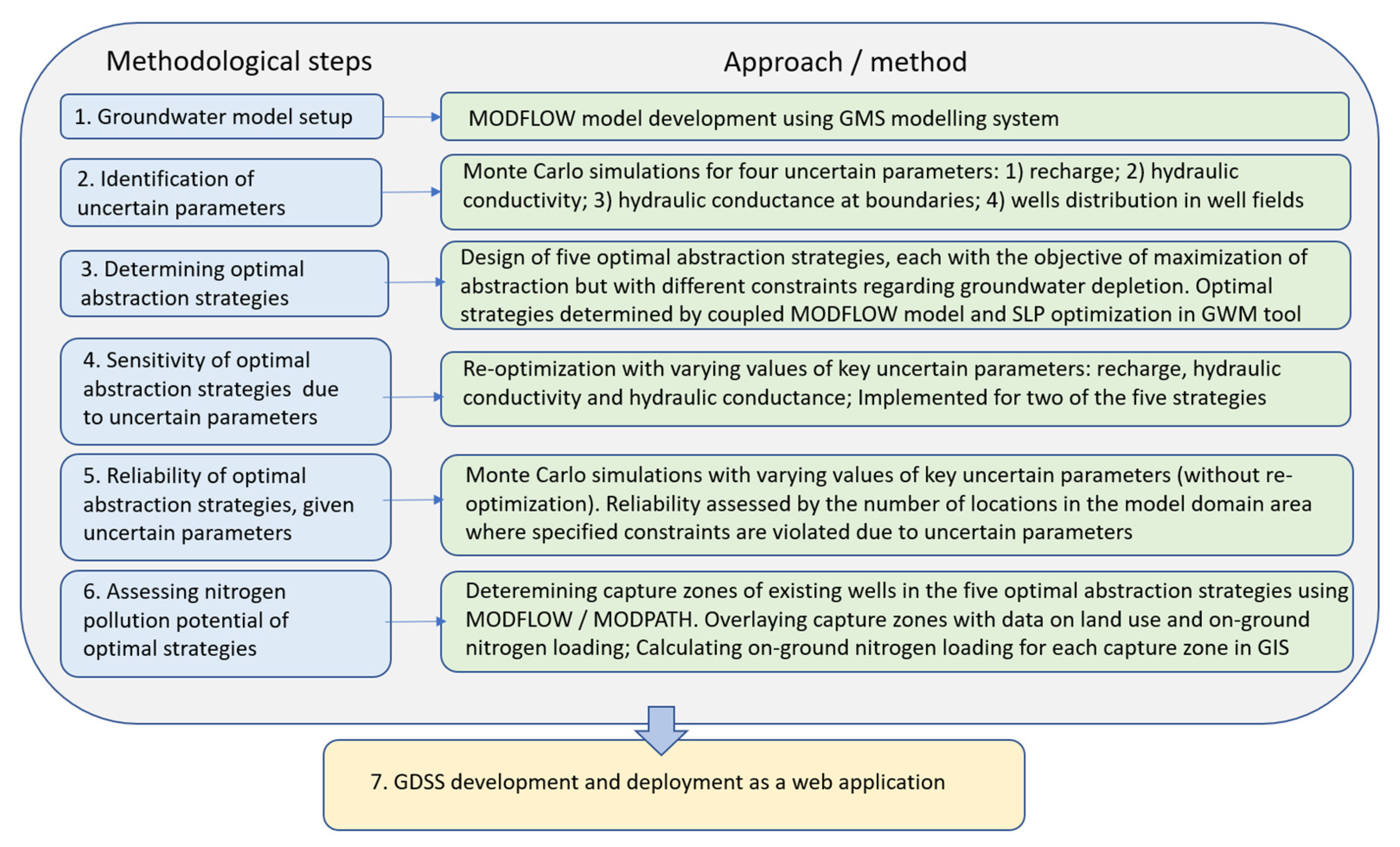
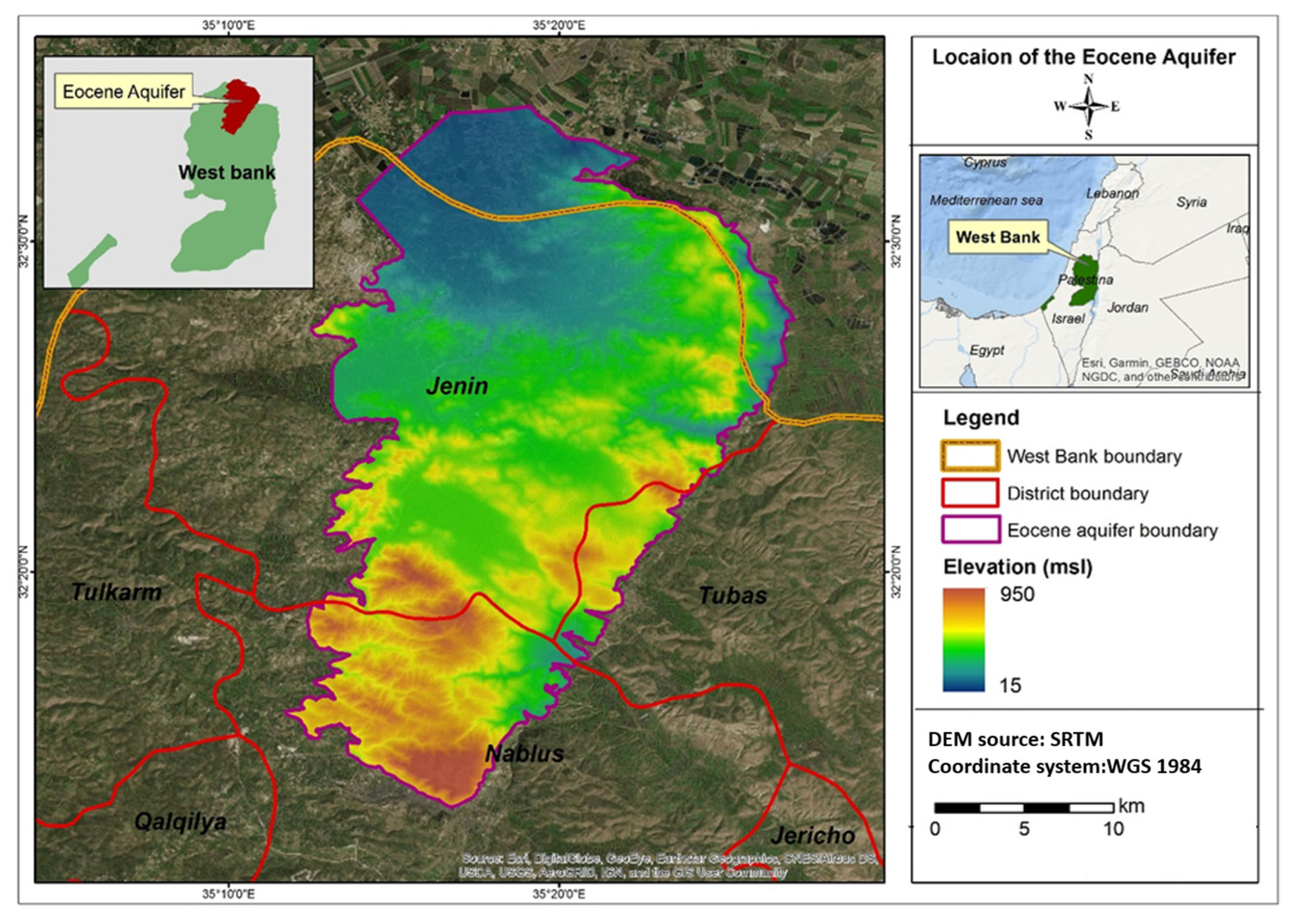
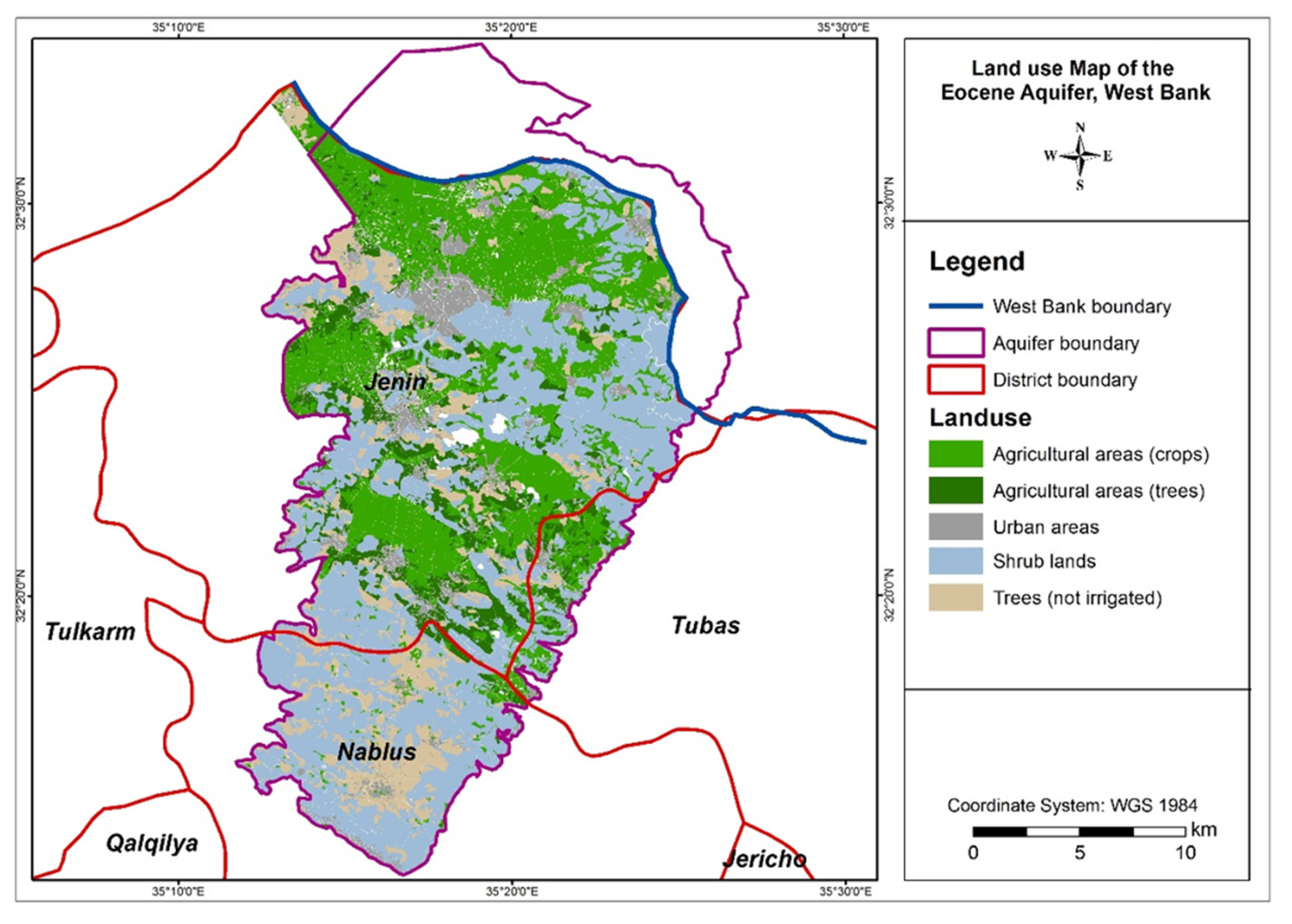
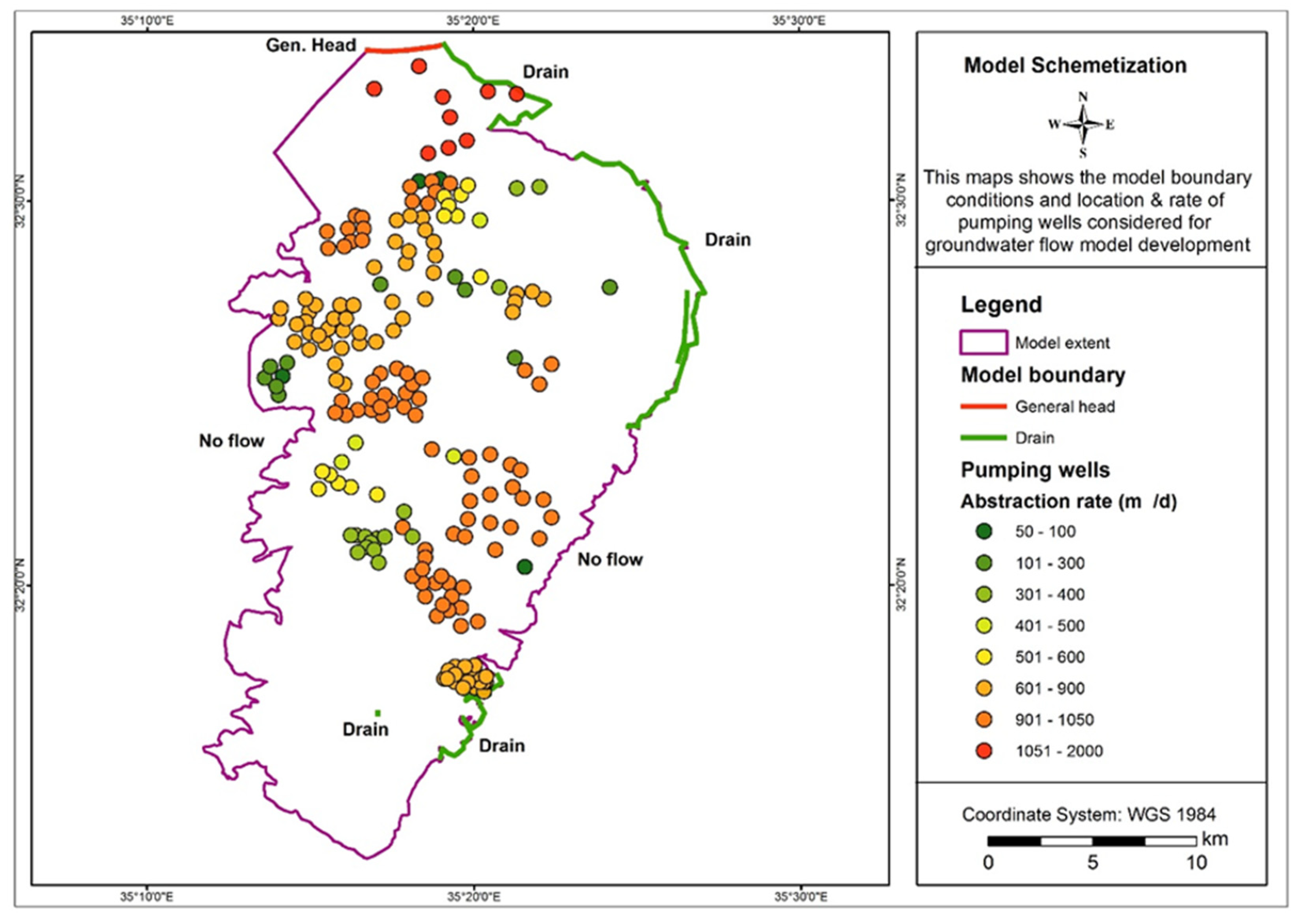
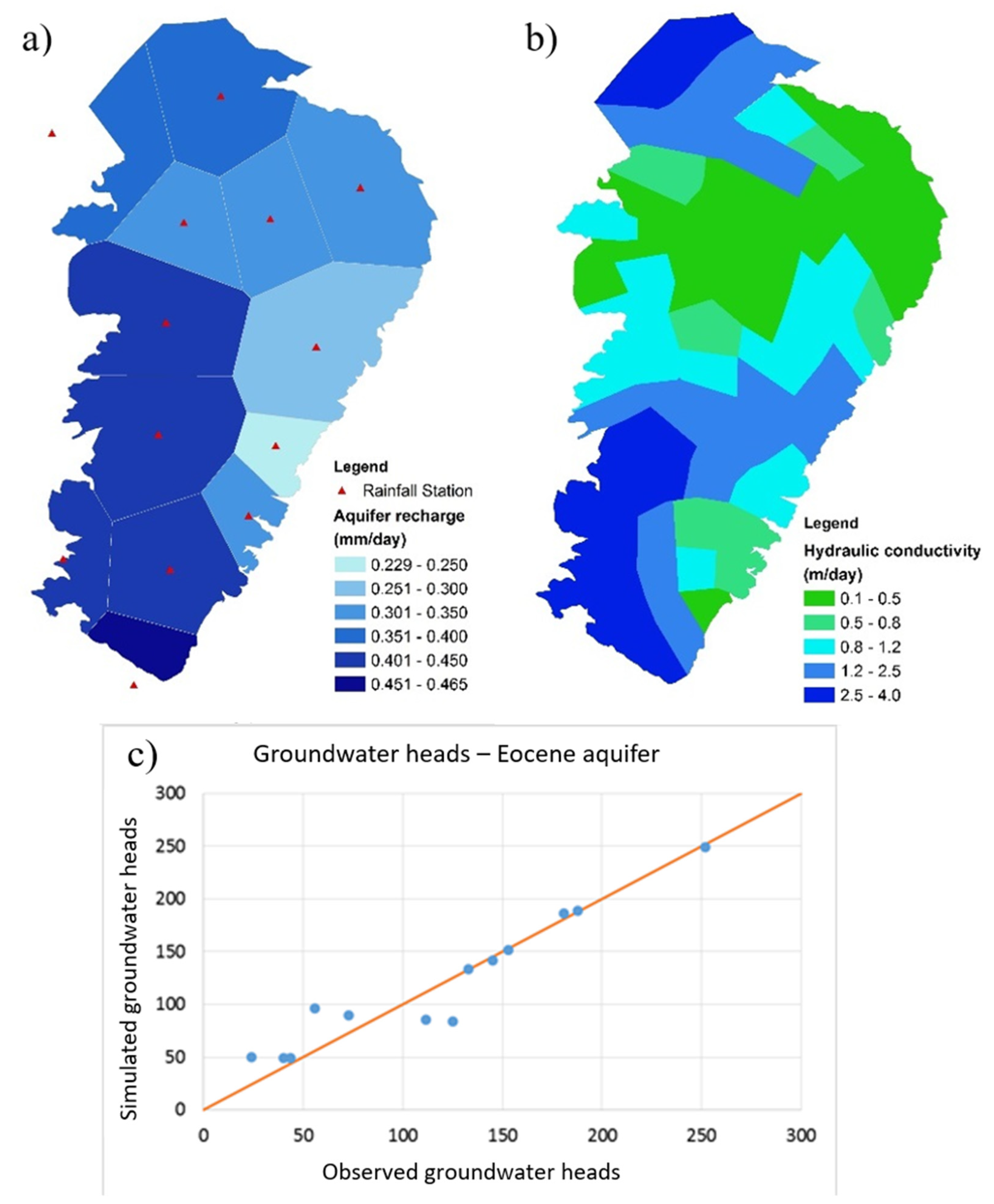
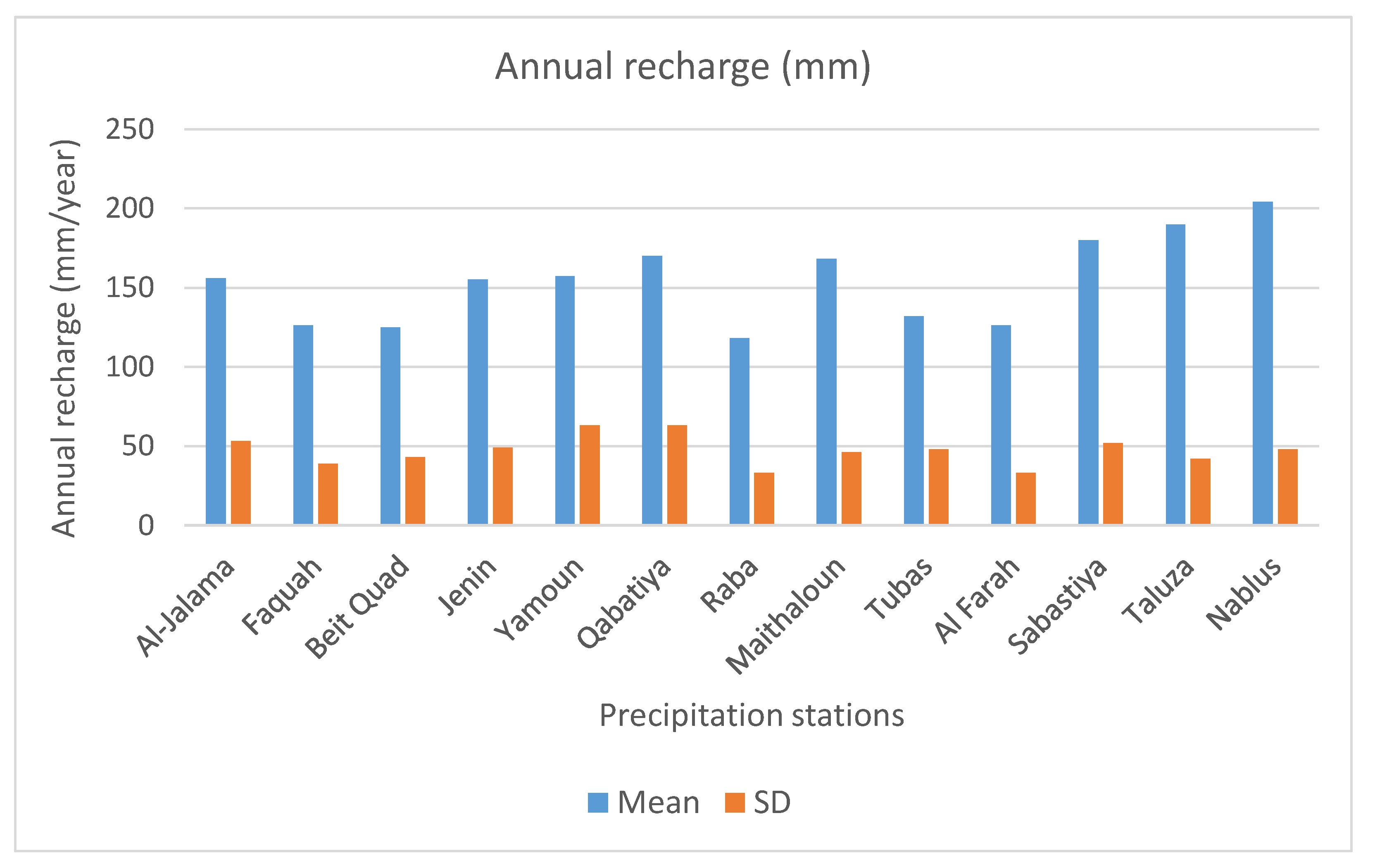
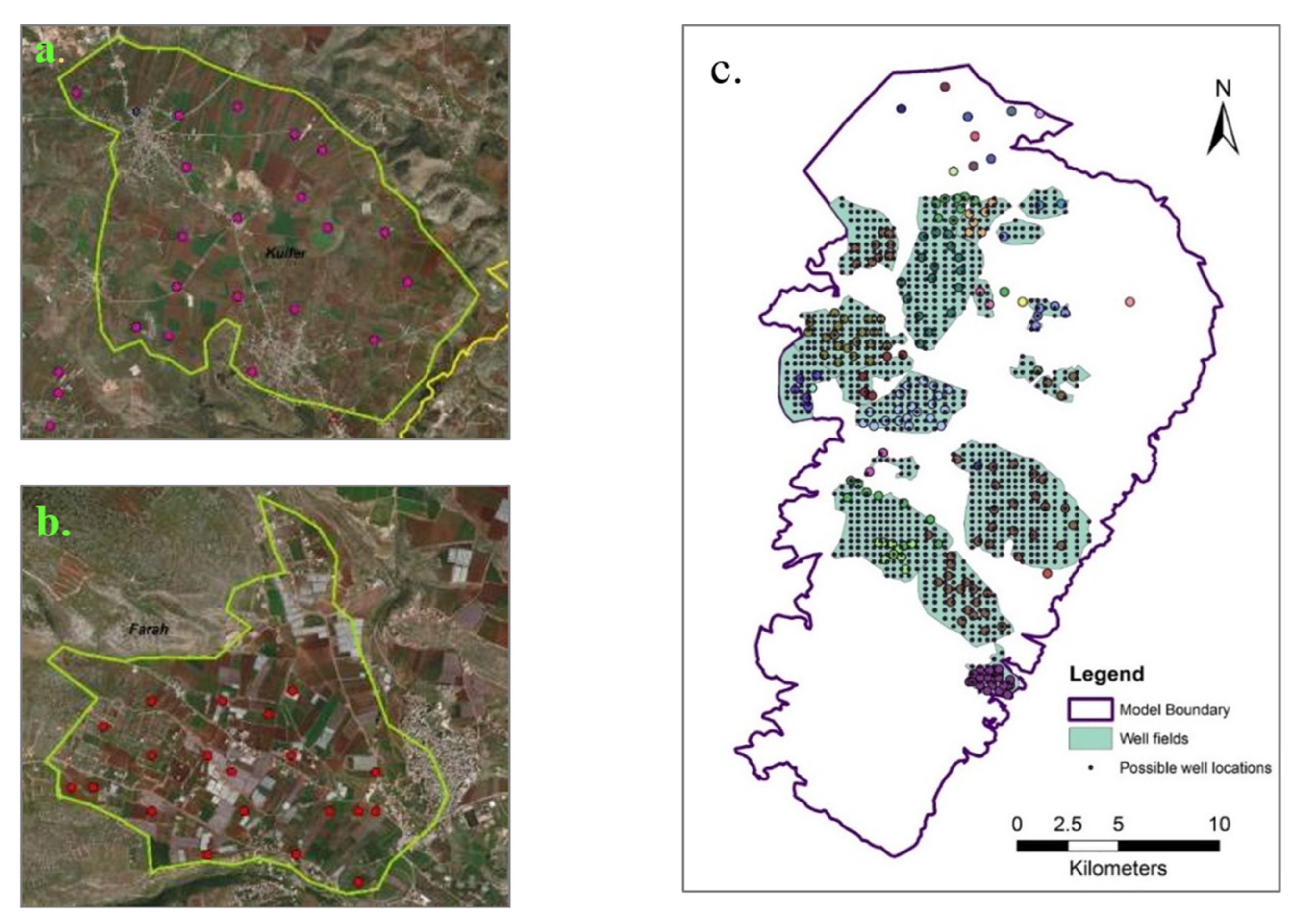
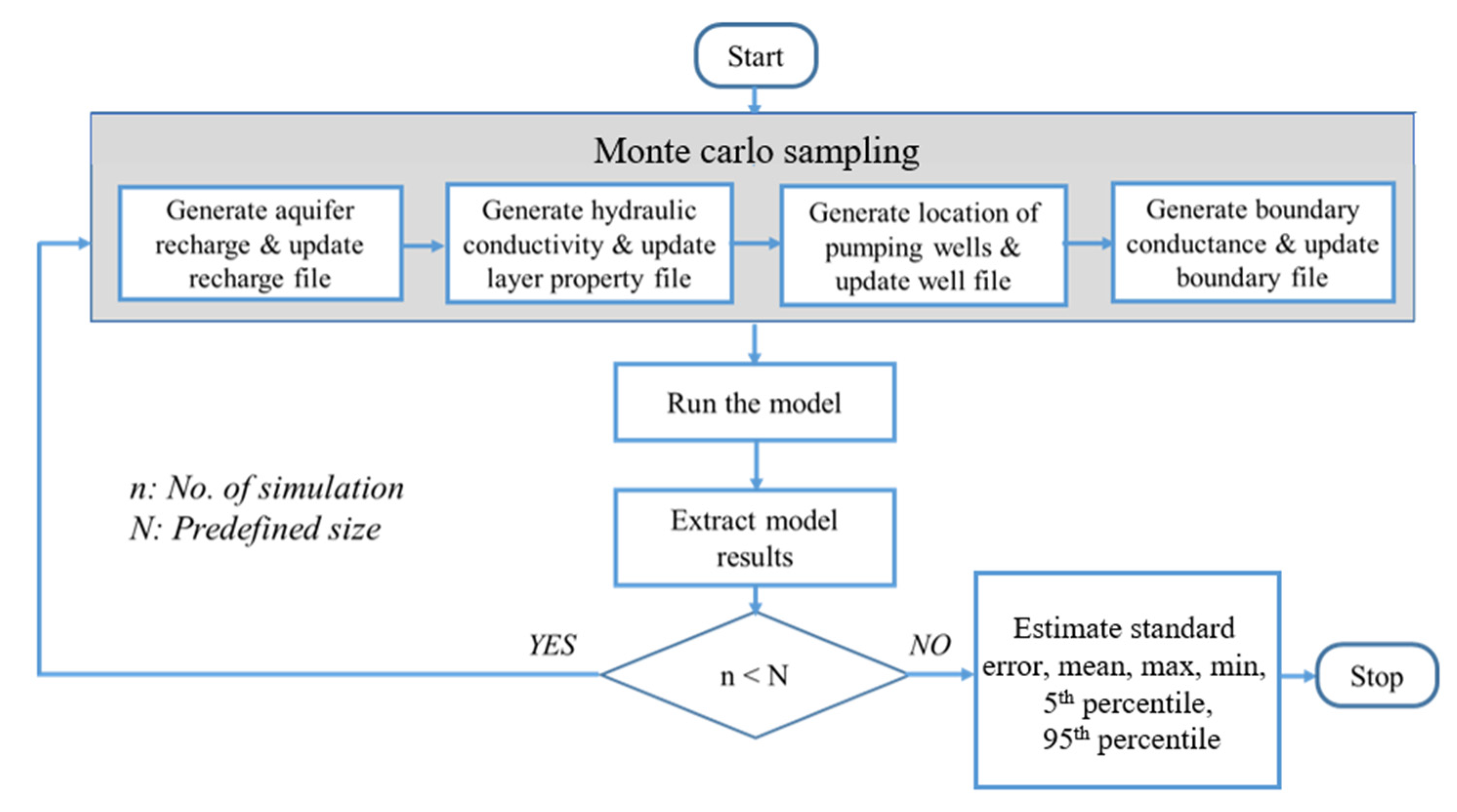
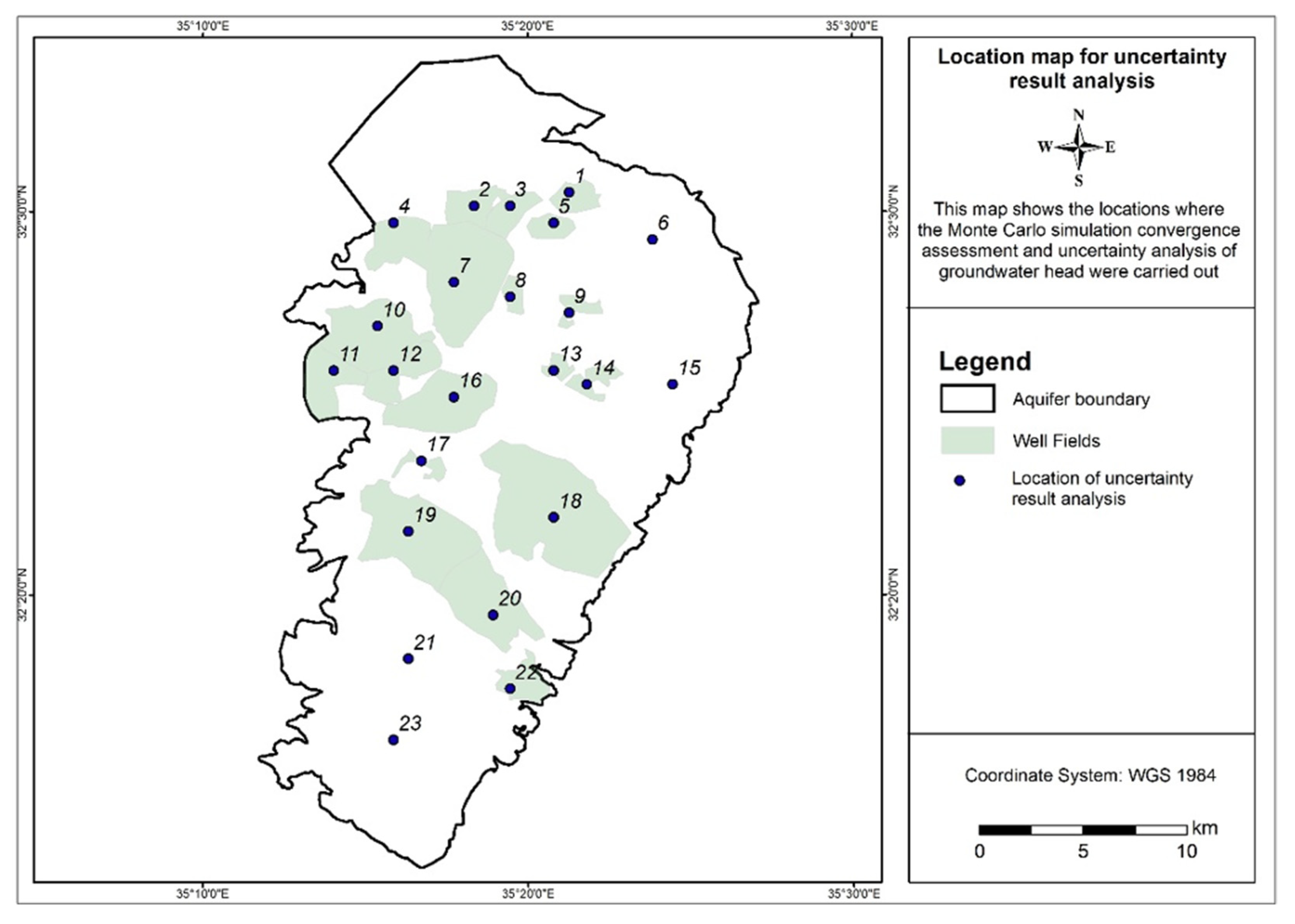
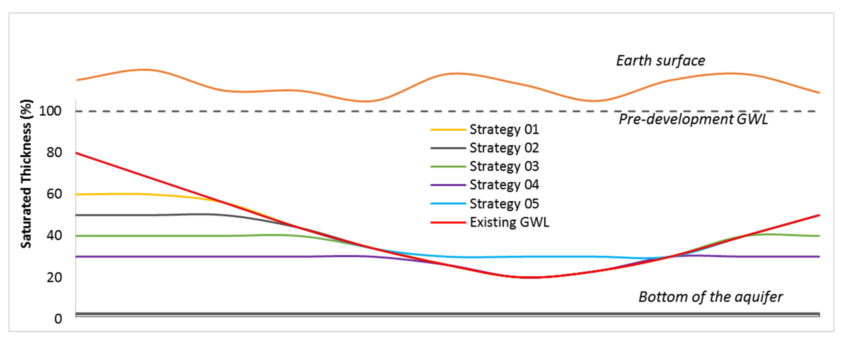
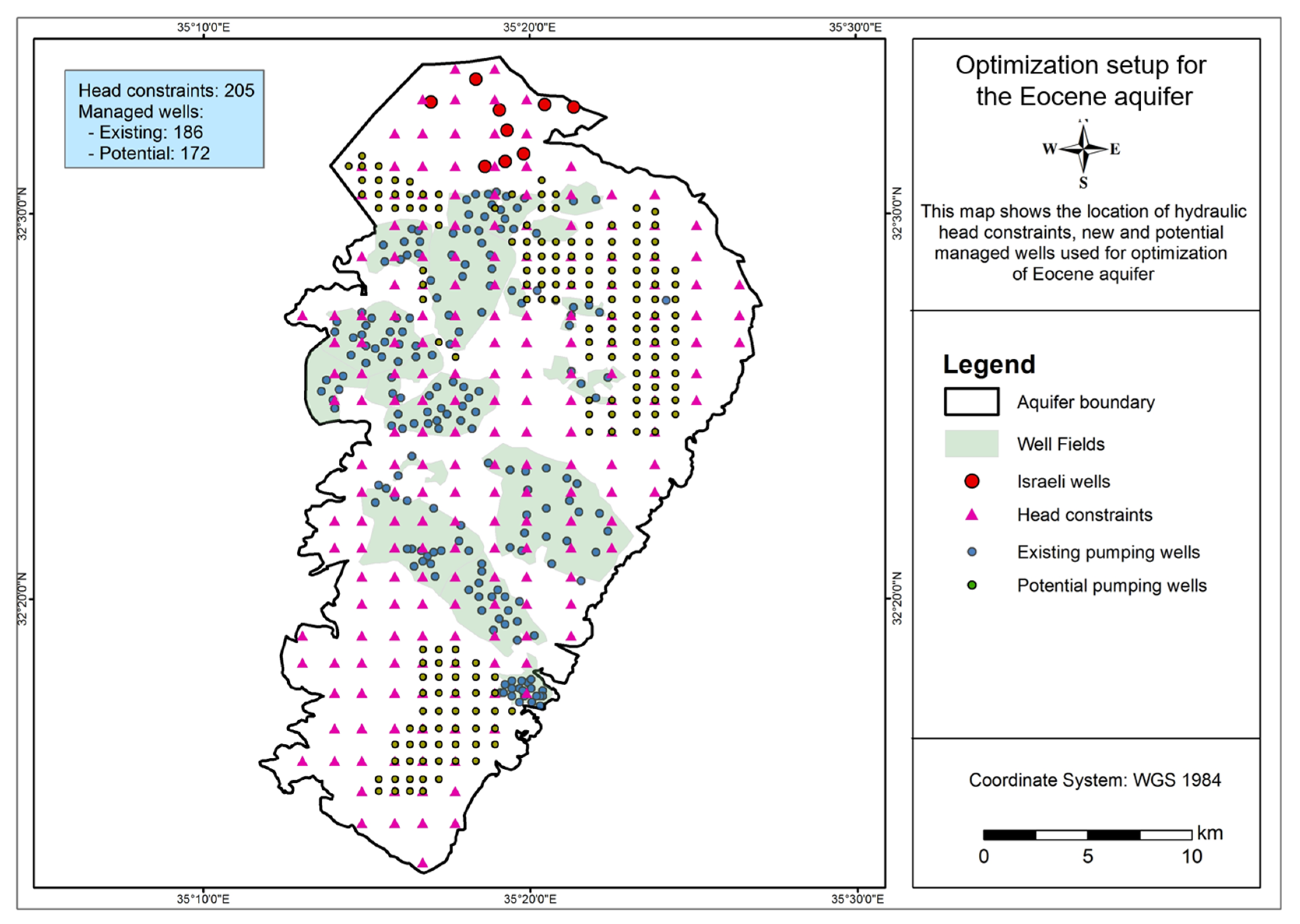
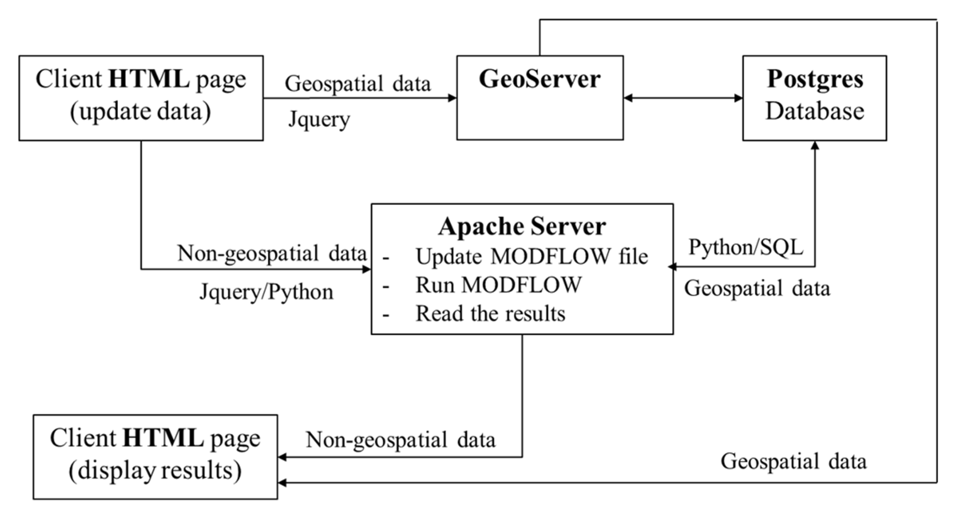
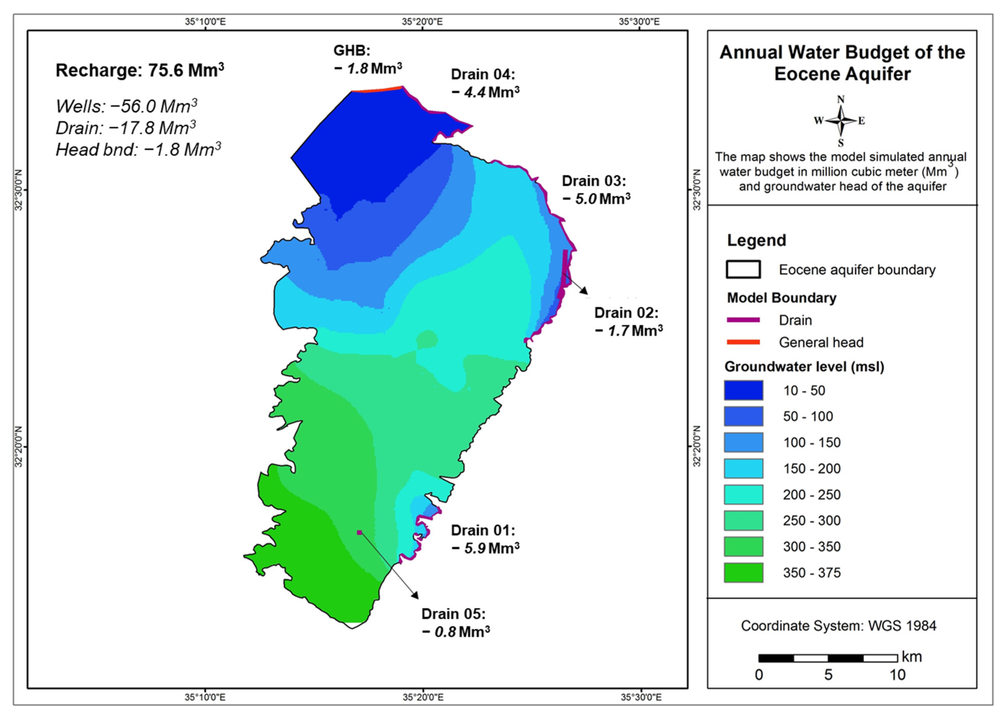
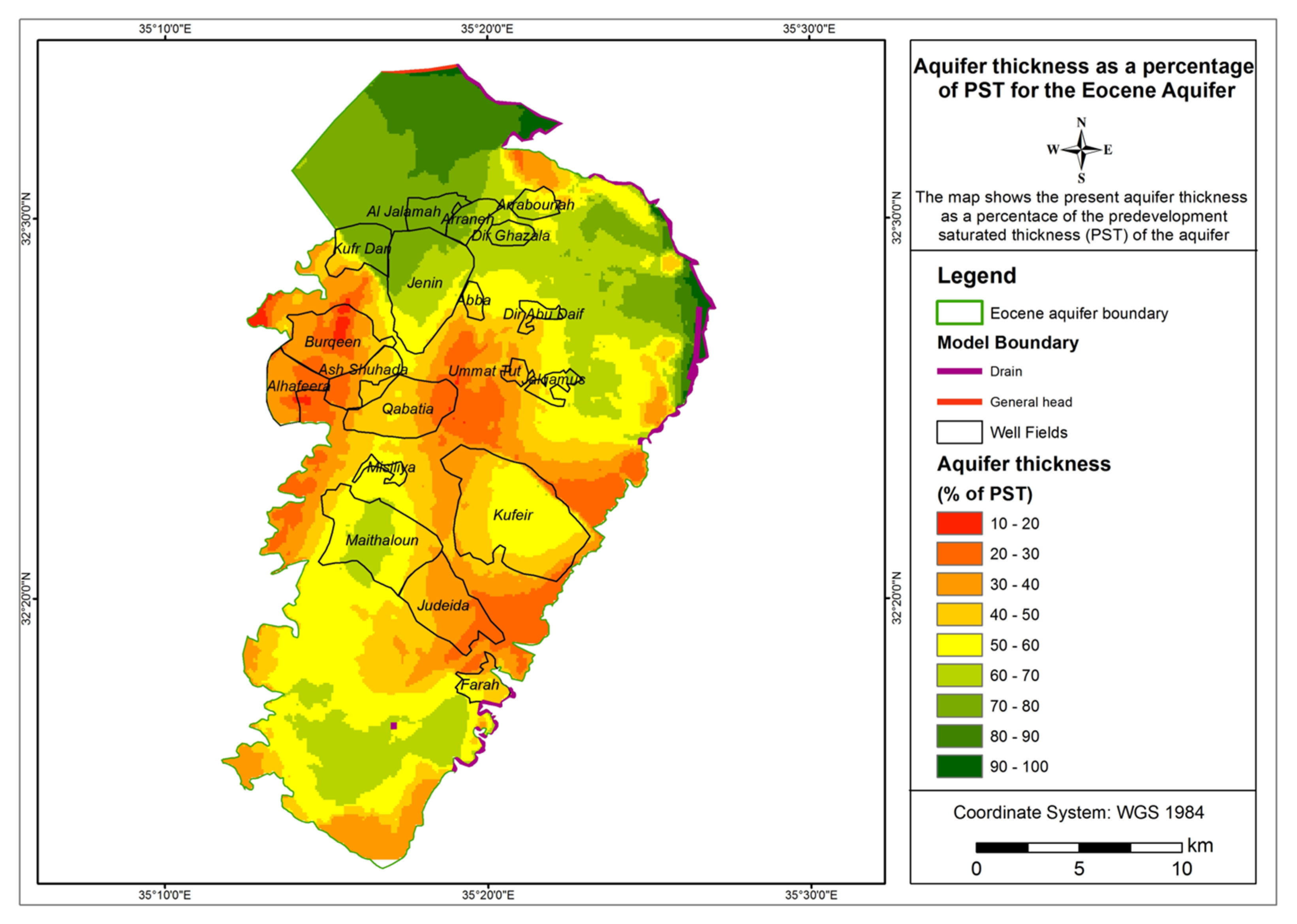
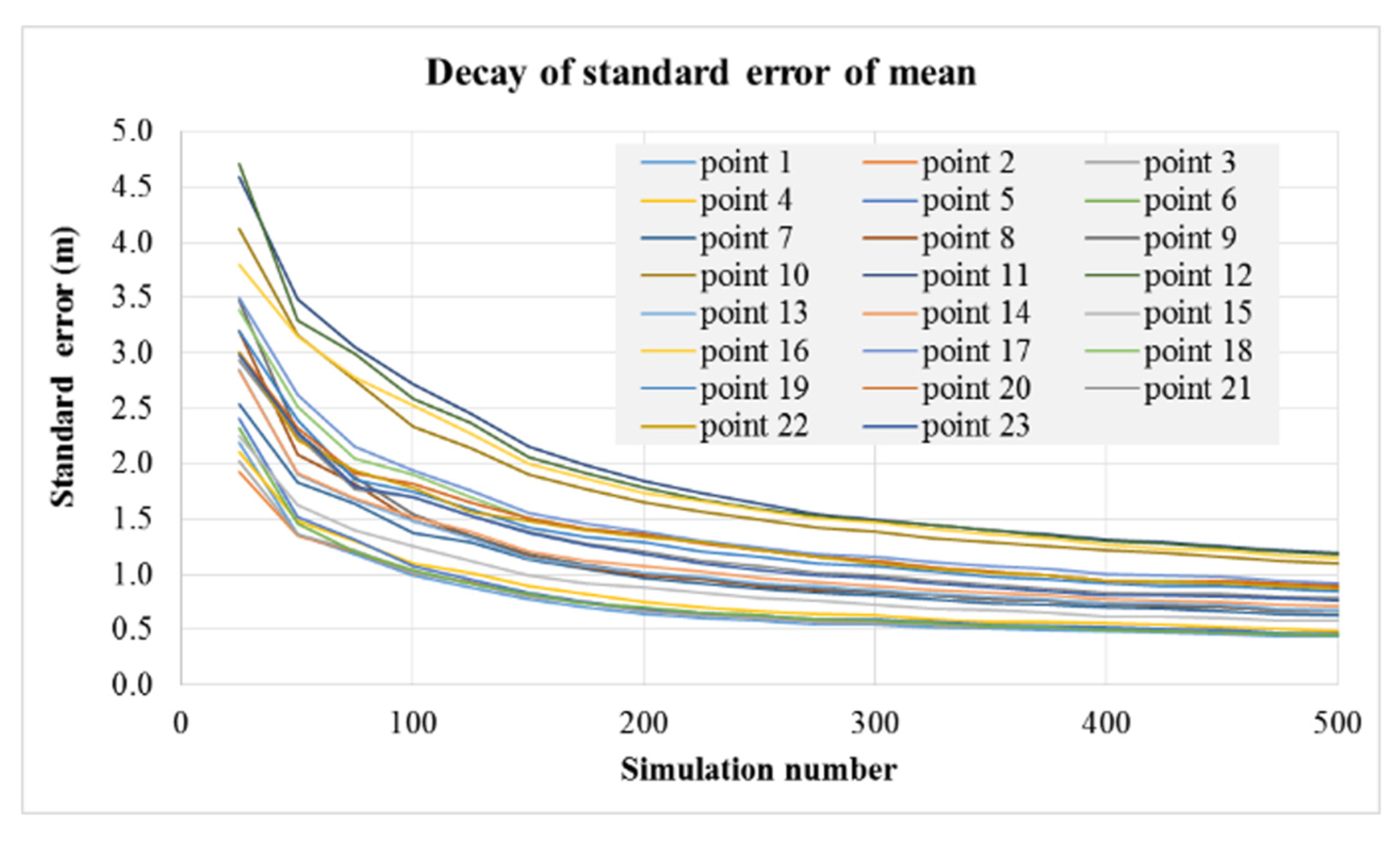
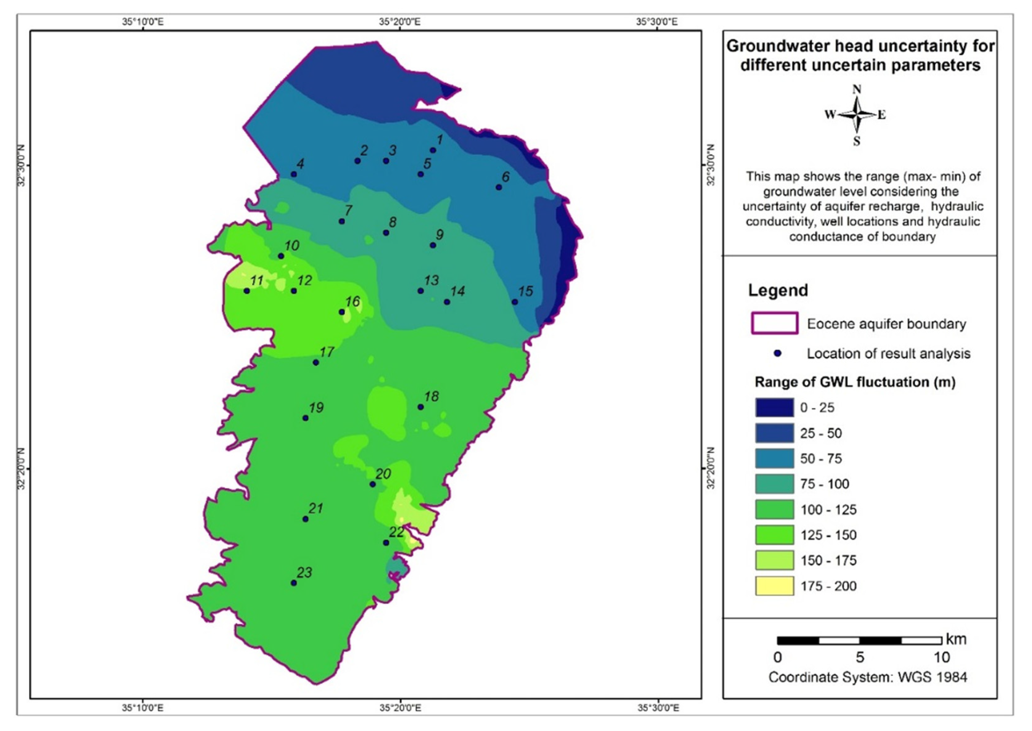
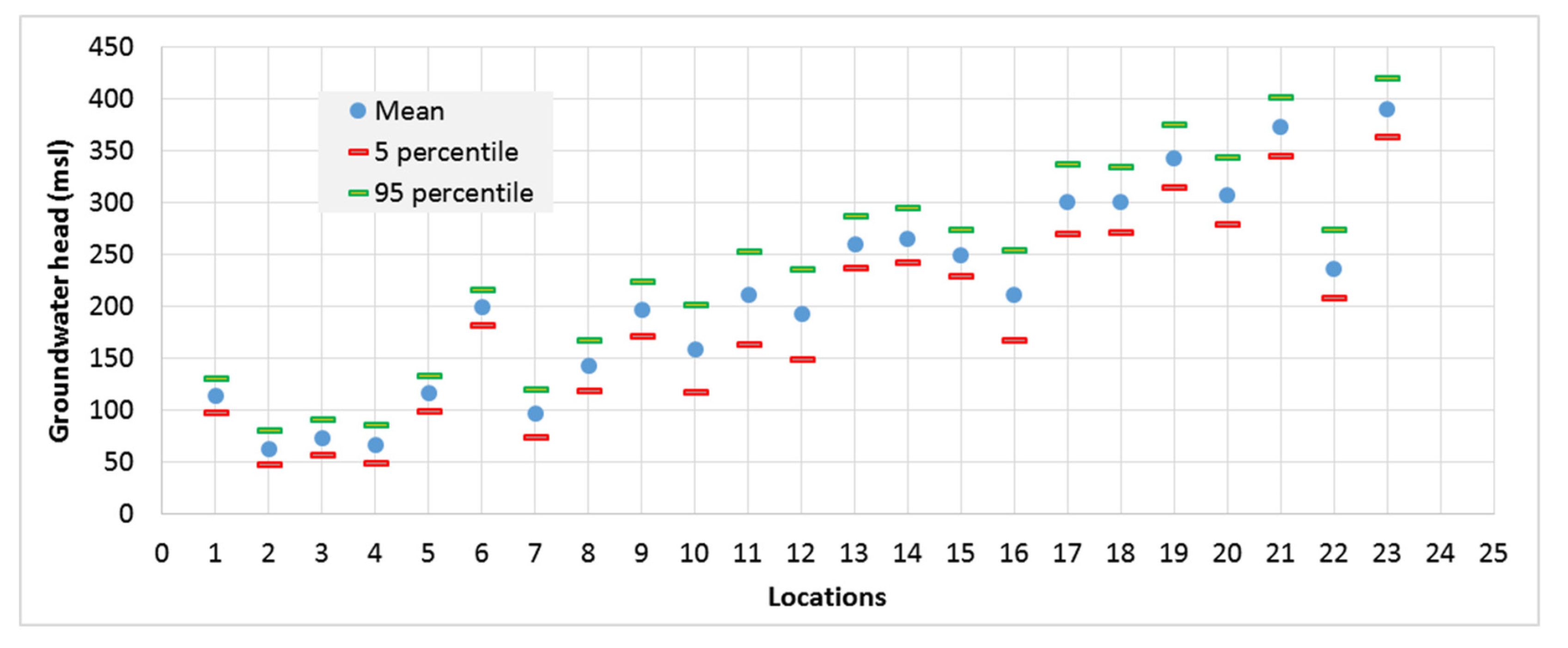
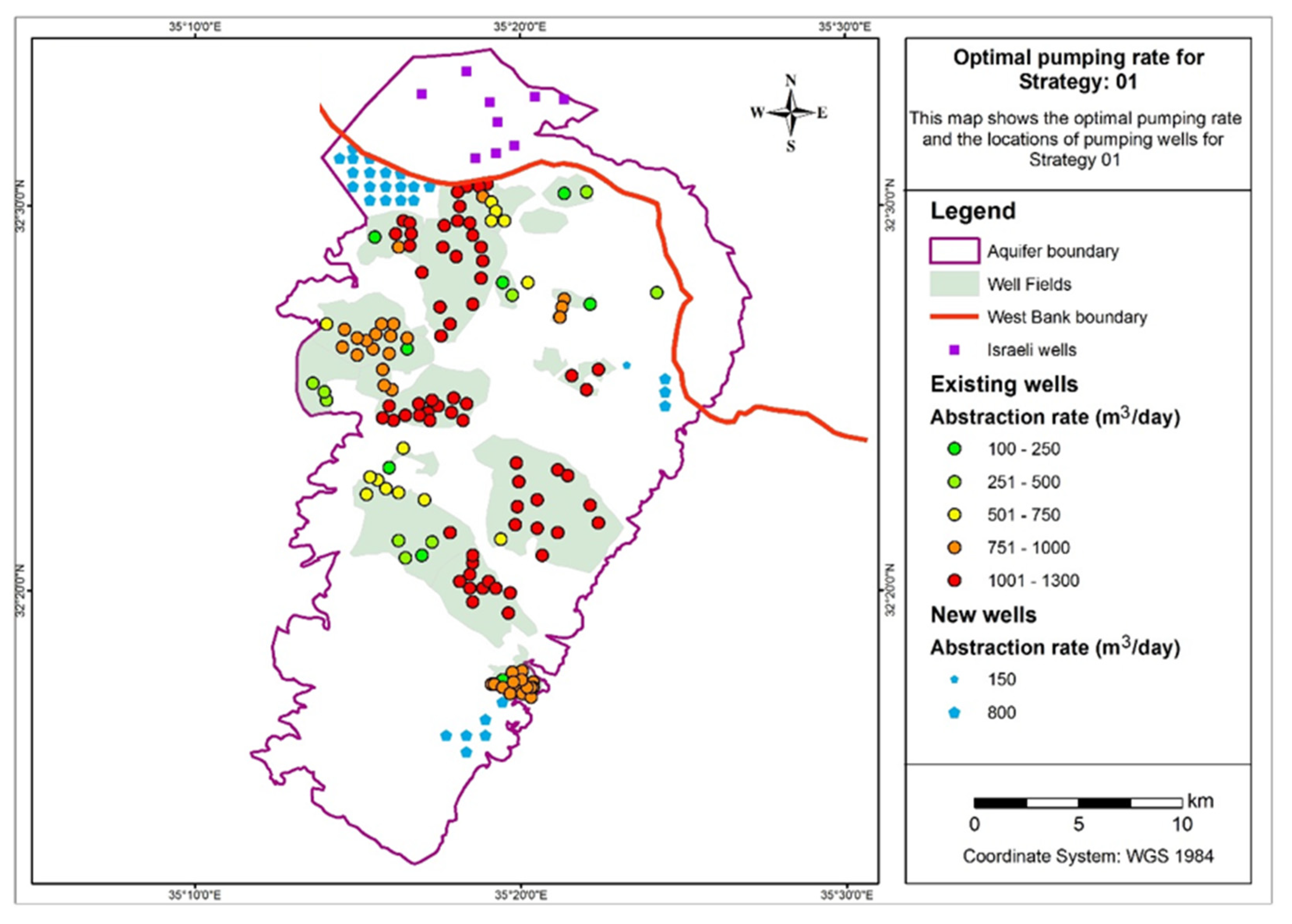
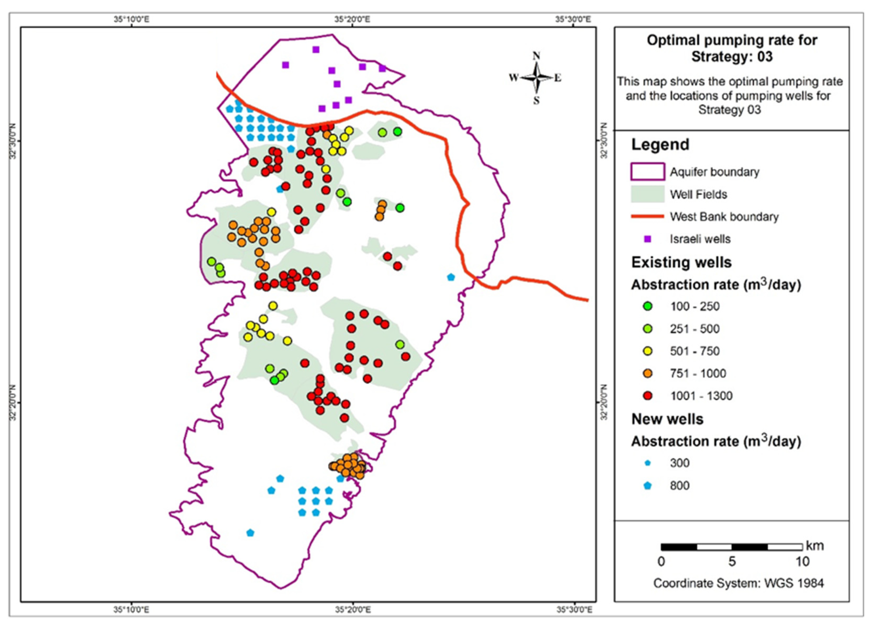
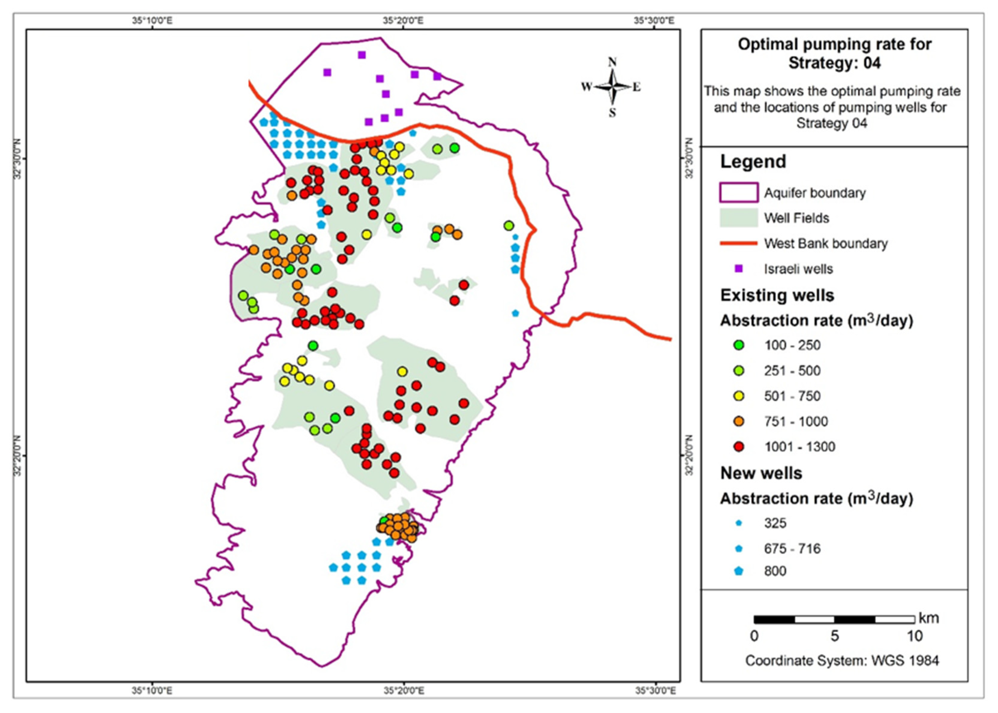
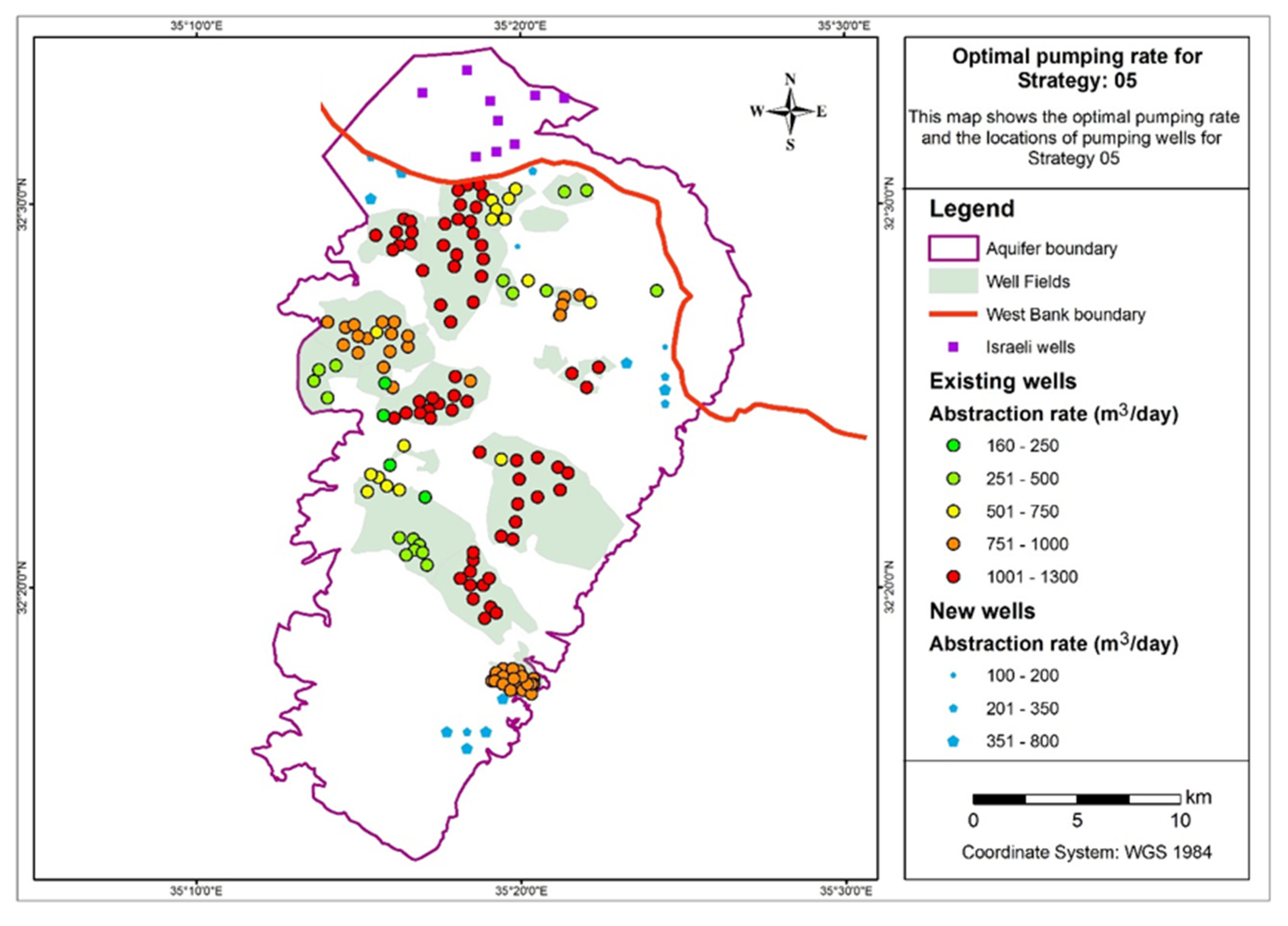
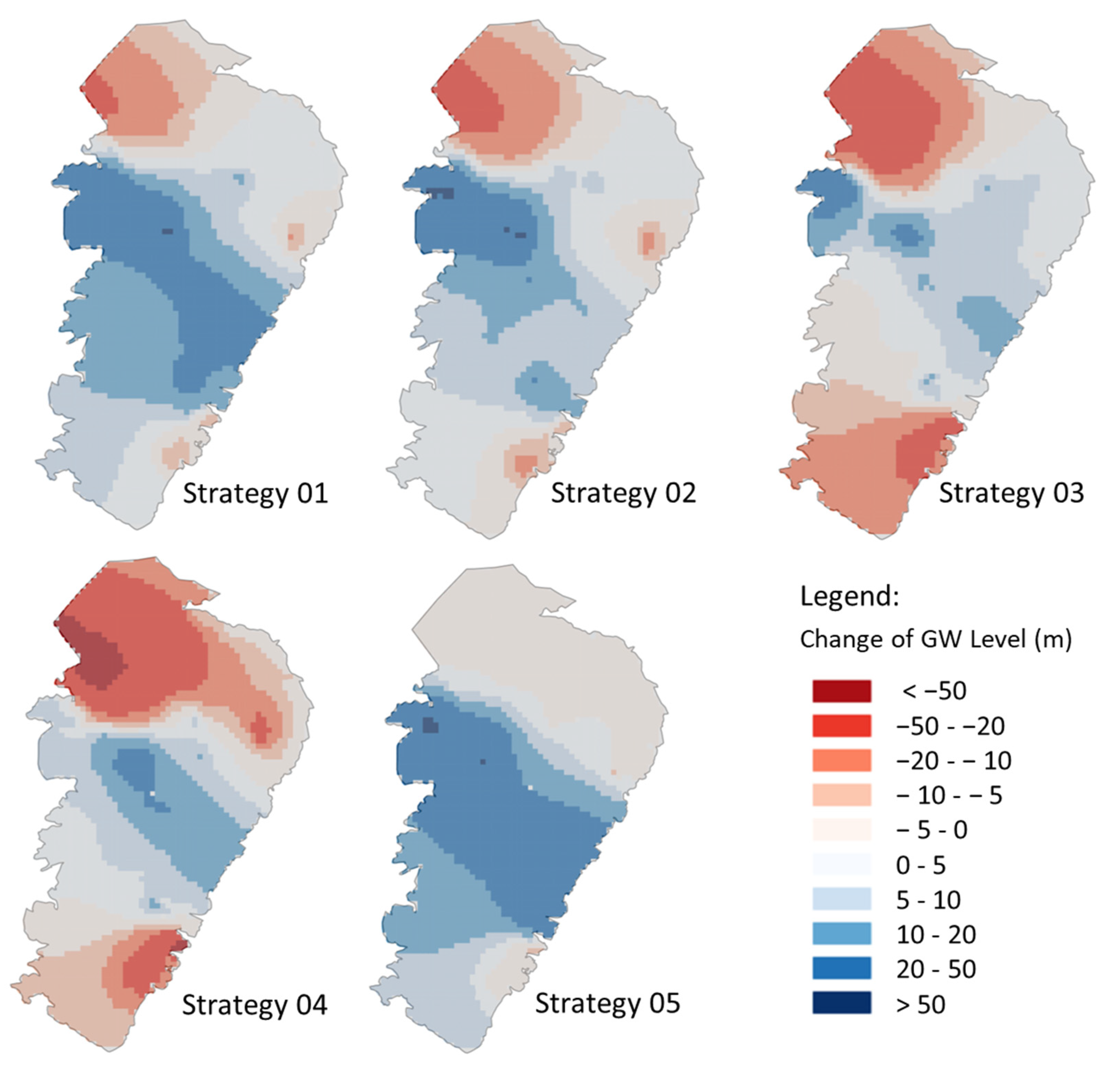
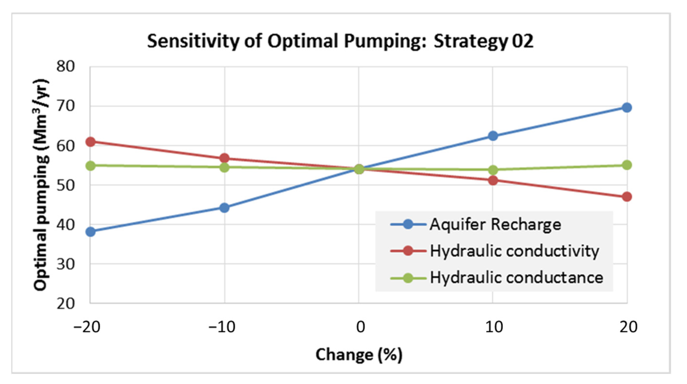
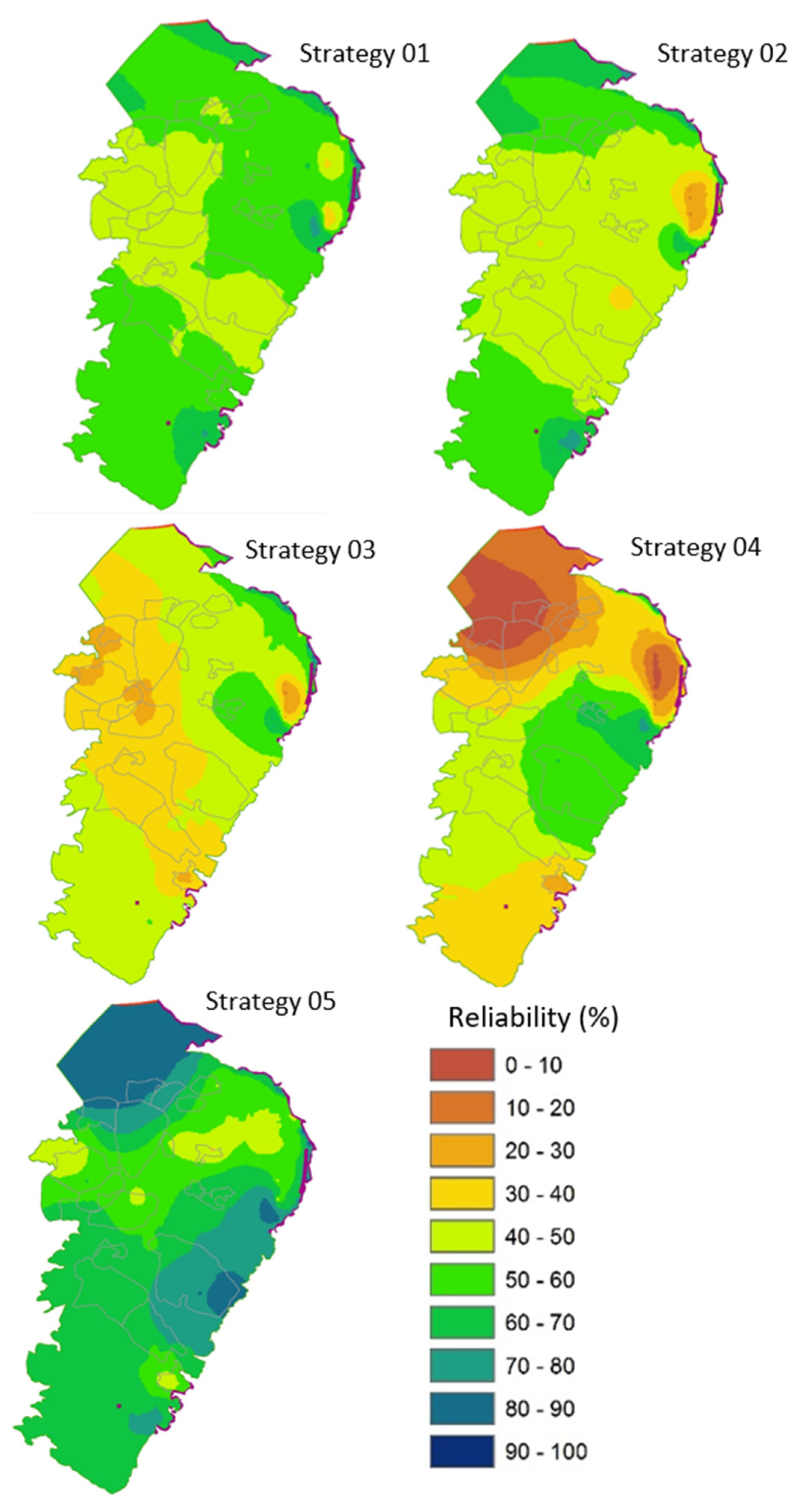
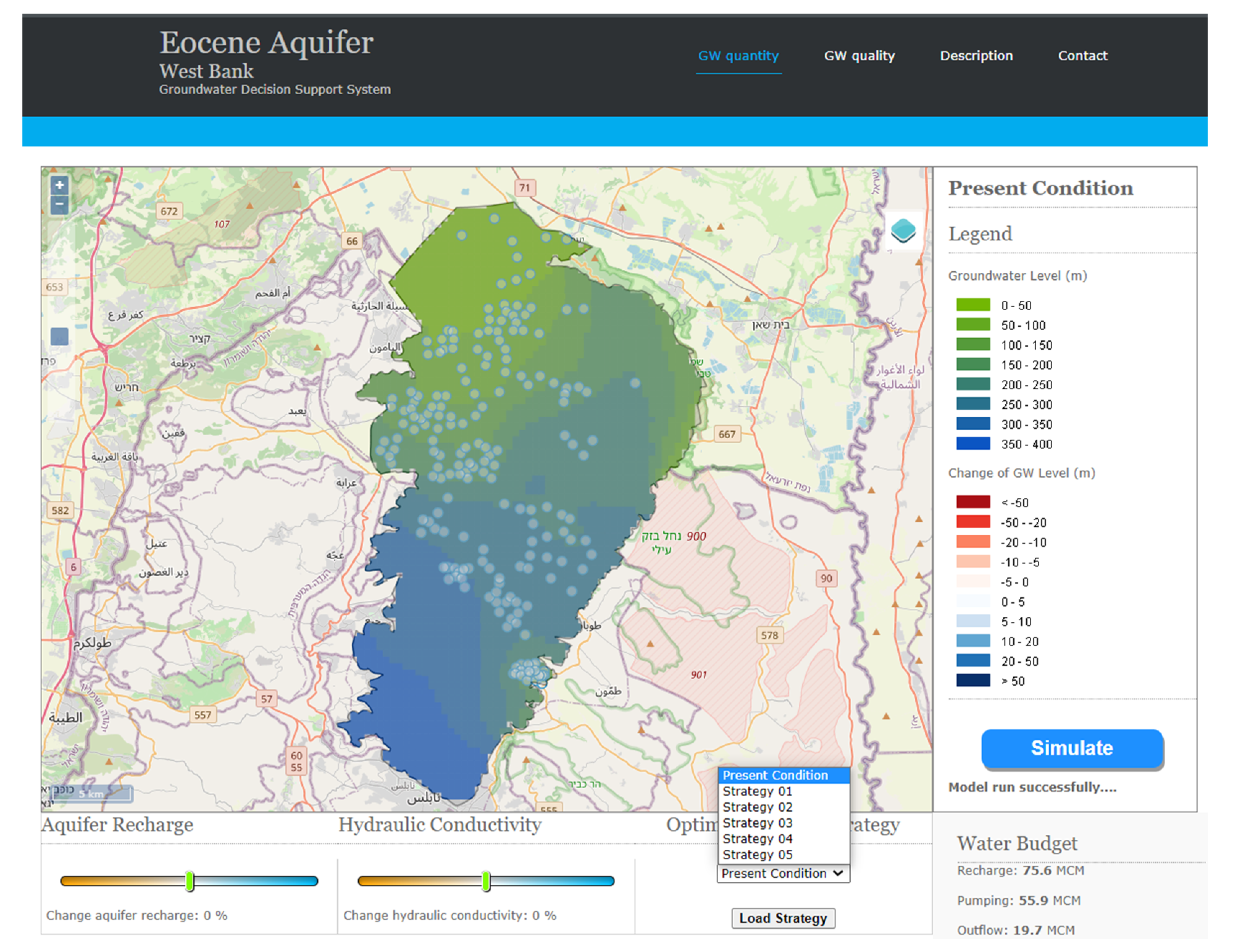
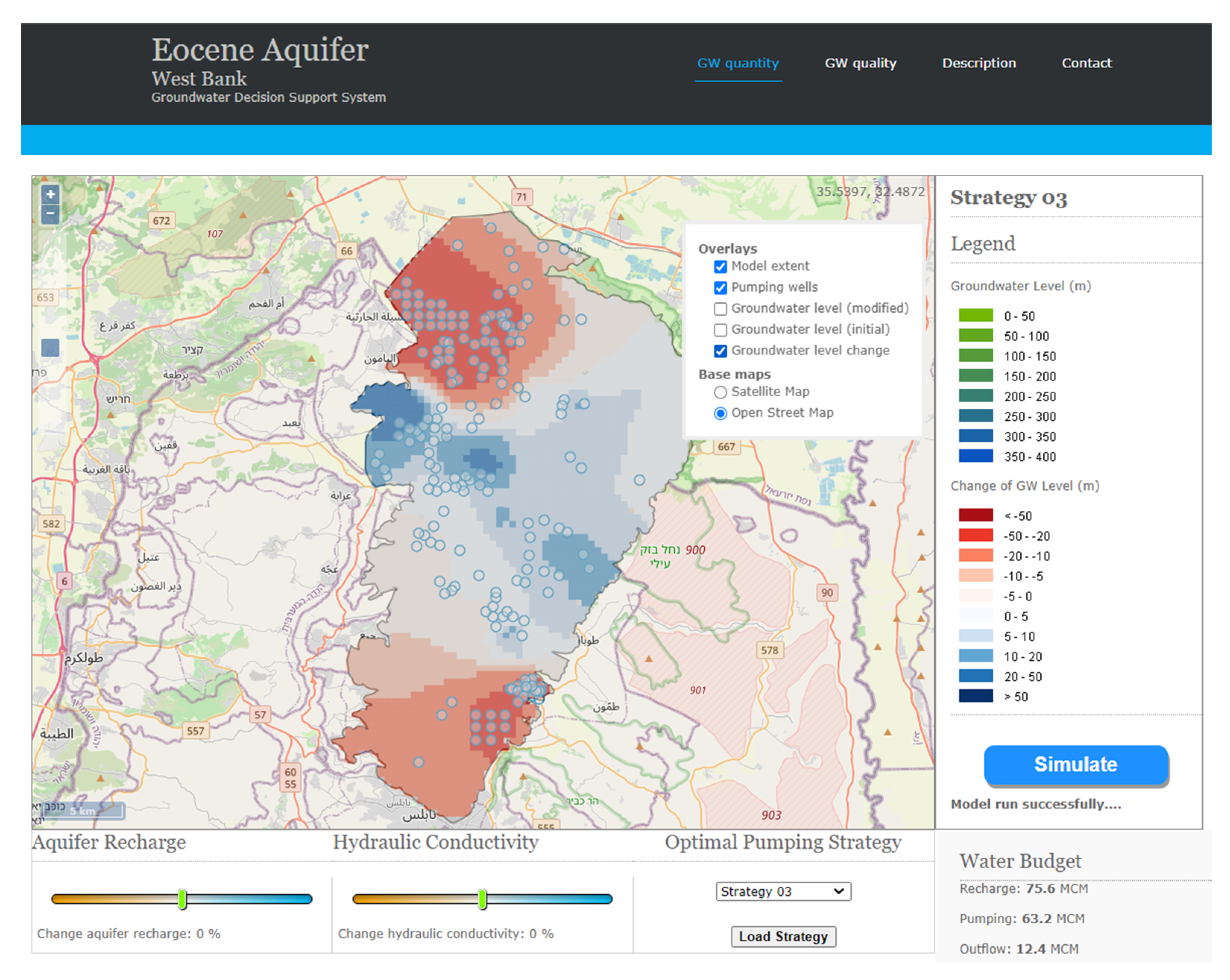
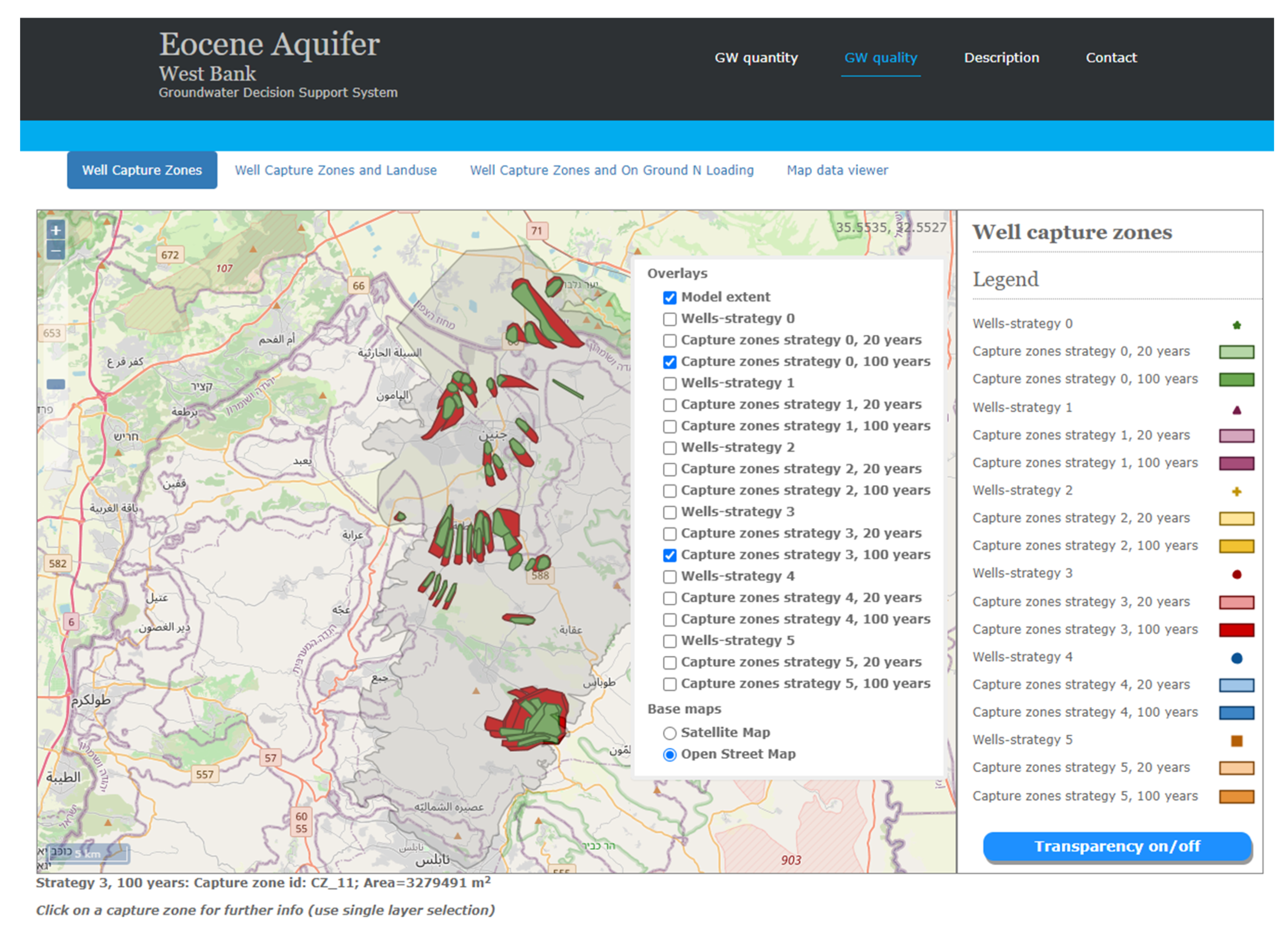
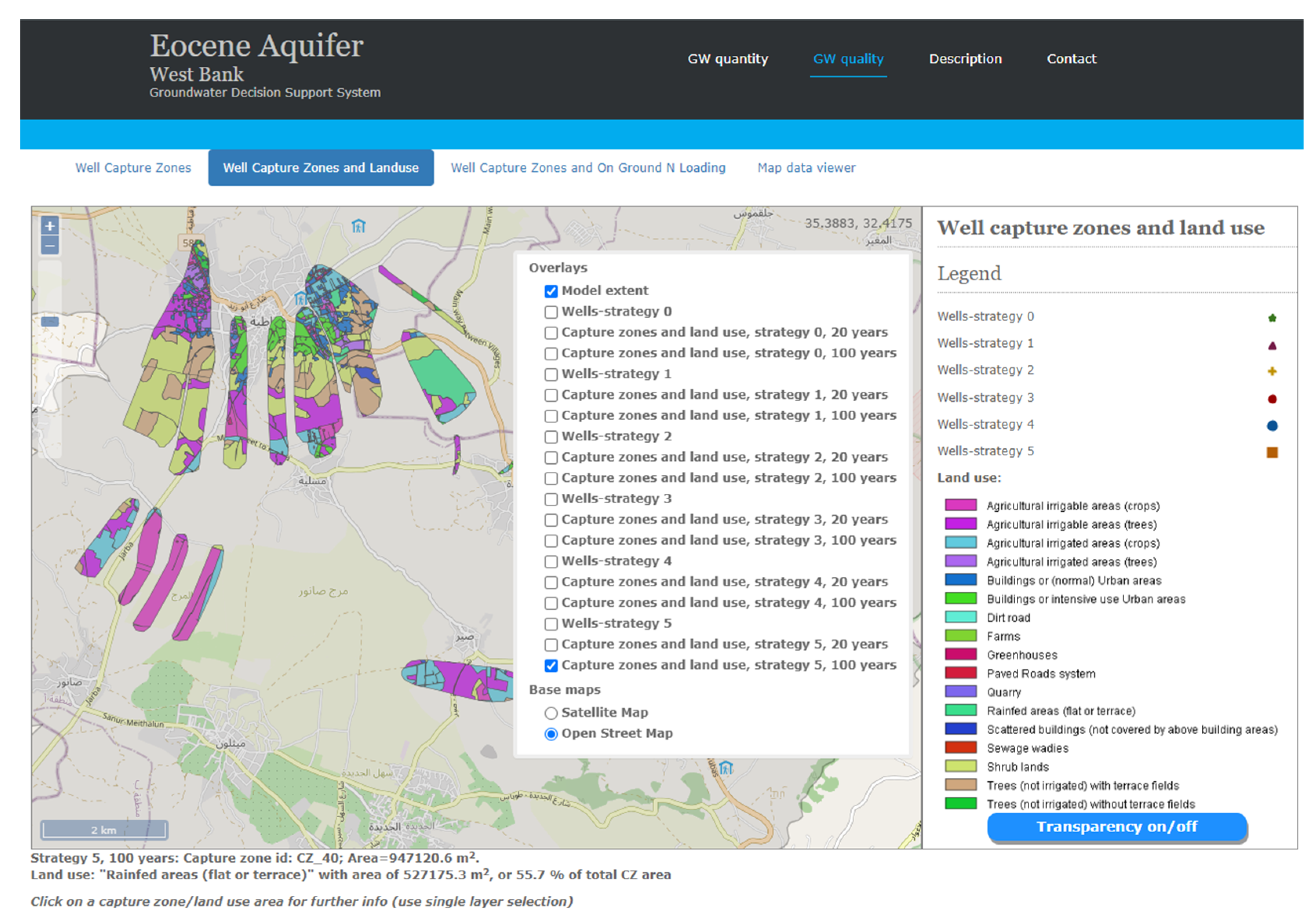
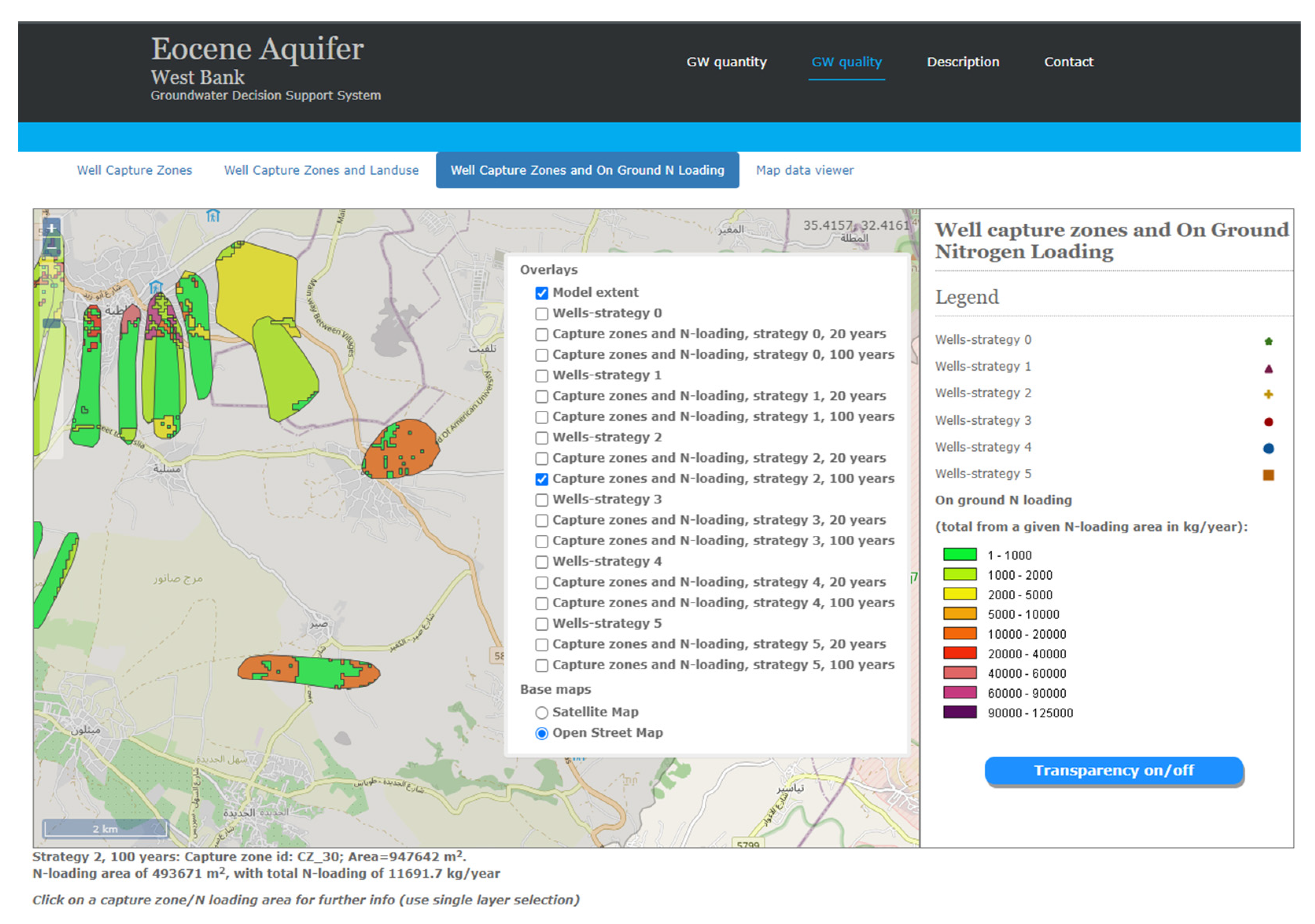
Table 1.
Total optimal abstraction for the five identified strategies.
| Strategy: | Existing | 01 | 02 | 03 | 04 | 05 |
|---|---|---|---|---|---|---|
| Total abstraction (Mm3/year) | 49.4 | 52.6 | 54.1 | 56.7 | 60.2 | 50.1 |
| Percentage increase (%) | - | 6.7 | 9.5 | 14.8 | 21.9 | 1.4 |
Disclaimer/Publisher’s Note: The statements, opinions and data contained in all publications are solely those of the individual author(s) and contributor(s) and not of MDPI and/or the editor(s). MDPI and/or the editor(s) disclaim responsibility for any injury to people or property resulting from any ideas, methods, instructions or products referred to in the content. |
© 2023 by the authors. Licensee MDPI, Basel, Switzerland. This article is an open access article distributed under the terms and conditions of the Creative Commons Attribution (CC BY) license (https://creativecommons.org/licenses/by/4.0/).
Share and Cite
MDPI and ACS Style
Jonoski, A.; Ahmed, T.; Almasri, M.N.; Abu-Saadah, M. Decision Support System for Sustainable Exploitation of the Eocene Aquifer in the West Bank, Palestine. Water 2023, 15, 365. https://doi.org/10.3390/w15020365
AMA Style
Jonoski A, Ahmed T, Almasri MN, Abu-Saadah M. Decision Support System for Sustainable Exploitation of the Eocene Aquifer in the West Bank, Palestine. Water. 2023; 15(2):365. https://doi.org/10.3390/w15020365
Chicago/Turabian StyleJonoski, Andreja, Tanvir Ahmed, Mohammad N. Almasri, and Muath Abu-Saadah. 2023. "Decision Support System for Sustainable Exploitation of the Eocene Aquifer in the West Bank, Palestine" Water 15, no. 2: 365. https://doi.org/10.3390/w15020365
Note that from the first issue of 2016, this journal uses article numbers instead of page numbers. See further details here.