
Optimum Coastal Slopes Exposed to Waves: Experimental and Numerical Study


1
Department of Energy Conversion Engineering, Faculty of Mechanical and Materials Engineering, Graduate University of Advanced Technology, Kerman 7631885356, Iran
2
Department of Water Engineering, Faculty of Civil and Surveying Engineering, Graduate University of Advanced Technology, Kerman 7631885356, Iran
*
Author to whom correspondence should be addressed.
Water 2023, 15(2), 366; https://doi.org/10.3390/w15020366
Submission received: 2 December 2022
/
Revised: 22 December 2022
/
Accepted: 9 January 2023
/
Published: 16 January 2023
(This article belongs to the Special Issue Erosion and Sediment Transport Processes in Coastal Waters)
Abstract
:In this research, experimental and numerical studies of water waves in a wave tank are analyzed and how to find the optimum beach slope for numerical simulation is also investigated. First, with the aid of a wave tank (flap type), waves with different wave amplitudes are created in the laboratory, and data of generated waves are measured by different wave probes. Then, numerical simulations of the wave tank and waves with different wave amplitudes are performed in Ansys Fluent industrial software. The VOF method is used to model two-phase flow. The results of experimental and numerical simulations are compared and examined. Moreover, the effects of the beach slope on the simulation are analyzed and compared with the experimental results to obtain the best slope. The results show that the numerical simulation, by using the appropriate beach slope, can properly model the experimental results with a low CPU time. Additionally, the 1:5 beach slope is considered the best slope that can dampen the energy of the waves and prevent their reflection.
1. Introduction
As the world’s population grows, energy demand is also rising. Fossil fuels and renewable energy are used to supply this energy. Fossil fuels are the main source for supplying these requirements, the use of which causes increases in CO2 and the temperature of the Earth. The European Union has pledged to reduce greenhouse gas emissions by 20% compared to 1990 by 2020 while improving energy efficiency by 20% and increasing the share of renewable energy by 20%. In October 2014, EU Energy agreed to reduce greenhouse gas emissions by at least 40% below 1990 levels by 2030 [1]. Renewable energies are divided into several different categories, one of which is the energy of sea waves. The energy of sea waves is also divided into several different categories, one of which is a point absorber. The point absorber transfers the energy of sea waves to linear generators, linear converters, mechanical rotors, or hydraulic pumps using a float that is much smaller than the wavelength [2].
To obtain this ocean wave energy and convert it into electricity, precise studies on sea waves and the interactions of these waves with wave energy converters (WECs) are required. A large number of studies have been performed to study various facets of quite a few methods that have been proposed for wave generation and the development of a numerical wave tank in the last few years. Lal and Elangovan [3] simulated a three-dimensional numerical wave tank using CFX Ansys software. They employed a flap-type wavemaker to produce waves to investigate the physical behaviors of the flap-type wavemaker by changing the governing parameters such as the dependency of the water fill depth, period of oscillations, and amplitude of oscillations of flaps.
Anbarsooz et al. [4] developed 2-D numerical wave tanks of flap and piston types. They found good agreement between the results of the flap- and piston-type wavemakers and experimental and theoretical ones. Later, Alamian et al. [5] simulated a two-dimensional numerical wave tank using the boundary element method. They applied a piston to generate nonlinear waves, and they additionally solved the equation of the free surface boundary condition by using the Euler–Lagrangian method. Ultimately, their findings indicated a well-matched coincidence between the results of the simulated numerical wave tank and the result of the analytical method.
Collins et al. [6] presented a series of novel metrics to evaluate the quality of the wave produced in the field. From their investigation, the results of quality metrics demonstrated that the physical aspects of the basin itself played a substantial role in controlling the accuracy and homogeneity of the wave. For example, they have shown how the homogeneity of wave height and period can be quantified. These methods can be extended and applied to all types of basins to allow potential basin users to determine whether a basin is suitable for their needs.
In the case of a multilevel breakwater for wave energy conversion, Han et al. [7] studied the numerical wave tank, based on the VOF model in Fluent software, in order to evaluate the overtopping wave energy converter (OWEC)’s performance. They employed two reservoirs with sloping walls at different levels as a multilevel breakwater, and consequently, the effects of the sloping angles of the two reservoirs and the gap height between the reservoirs were numerically investigated. They found that the smaller opening width, the larger height ratio, and the sloping angle of 30 degrees have positive effects on the performance of the system.
Wu and Hsiao [8] recruited two numerical methods (i.e., first-order wave solution by using the Dirichlet boundary condition and the ninth-order wave solution with the internal mass source) for wave generation. From their findings, the ninth-order wave solution with the internal mass source was more accurate. Later, Dao et al. [9] employed a 3-D numerical wave tank by using Open Foam software. They used the piston and flap wavemaker to generate waves and to dampen them. Ultimately, they concluded that the numerical wave tank model had high performance in terms of accuracy to validate experimental results. Houtani et al. [10] successfully simulated waves using a newly developed method called high-order spectral method wave generation (HOSM-WG). Additionally, Li et al. [11] compared the performance of three wave modeling methods (i.e., the internal wave generator method, the relaxation zone method, and the explicit spectral wave Navier–Stokes equations (SWENSE) method) as two-phase CFD solvers. The simulation results have been compared with the available experimental data obtained from model testing in the Ecole Centrale de Nantes Ocean engineering reservoir. The comparison showed the efficiency and accuracy of these wave modeling methods.
Hu et al. [12] employed the finite difference method of the numerical wave tank to solve two-dimensional Navier–Stokes equations in order to simulate the free surface flows. The simulation results were verified against the theory of high-order rational solutions of the Schrödinger cubic equation. Lv et al. [13] used an improved wavemaker velocity boundary condition (IWVBC) with the help of a reverse flow at the wave generator boundary. Using theoretical analysis, the phenomenon of mass conservation of waves was investigated randomly, and additionally, regular and different modes of mass transfer were found. IWVBC and the traditional wavemaker velocity boundary condition (TWVBC) were compared with reference data using computational fluid dynamics.
In the field of wave interaction with floating or fixed structures, several numerical simulations have been developed over the last decade. Westphalen et al. [14] used a numerical wave tank to simulate wave interaction on offshore structures (e.g., horizontal and vertical cylinders). They found that numerical results could accurately simulate the horizontal and vertical forces applied to the cylinders. Kim et al. [15] successfully validated experimental studies using Fluent commercial software in order to understand the mechanism of wave interactions with a fixed offshore substructure. The mesh independence test was performed on the number of meshes, which provided optimal conditions for numerical wave generations. Moreover, they found that wave damping affected the length of the damping domain.
Hu et al. [16] could create new boundary conditions for the wave using Open FOAM in order to simulate the wave interaction with a fixed/floating cylinder. In their research, a fixed horizontal and vertical cylinder and a floating cylinder were exposed to the waves. Additionally, In Bruinsma et al.’s [17] investigation, extensive validation of a fully nonlinear numerical wave tank was performed to accurately simulate the dynamic motion response of a rigid complex fluid structure and its interaction with floating bodies, based on recent experimental results of the OC5 floating offshore wind turbine subjected to waves. Tian et al. [18] simulated 3-D numerical wave tanks to investigate wave propagation and hydrodynamic forces based on the Navier–Stokes equations using Fluent software. From their research, the interactions of the wave with a vertical cylinder for different wave heights and wave periods were accurately validated. Moreover, Martínez-Ferrer et al. [19] successfully simulated a 2-D numerical wave tank with piston and flap types while considering the interaction waves with floating cylinder and cube structures. As a further investigation, Anbarsooz et al. [20] prosperously investigated the effects of the front wall inclination angle on the hydrodynamic performance of the oscillating water column by using a fully nonlinear two-dimensional numerical wave tank in Fluent software.
Kim and Kim [21] used a three-dimensional and fully nonlinear numerical wave tank (NWT) to analyze the interaction between nonlinear waves and stationary or floating bodies with uniform flow. NWT is based on the potential flow theory and boundary element method and simulates nonlinear wave–current–body interactions using mixed Eulerian and Lagrangian (MEL) methods. Vertical cylinders fixed at the bottom and cut in waves and currents were simulated, and the forces of wave launch, wave frequency, dual frequency, and mean drift were calculated and compared with published results using the second-order perturbation approach.
Over the last decade, a wide range of efforts has been made to investigate the effect of slope beaches on wave production in a wave tank [22,23,24,25,26,27]. Finnegan and Goggins [22] developed a numerical wave tank using Ansys CFX software while applying a flap-type wavemaker. To investigate the reflection of the wave after approaching the coast, different coastal slopes were considered, and additionally, the 1:5 slope was selected as the best slope.
Zabihi et al. [23] simulated a numerical wave tank with the same dimensions and properties using Fluent software and Flow-3D software. The obtained results of free surface elevation and the horizontal component of wave particle velocity from both software were successfully compared with the theoretical results. Additionally, the results showed that Flow3D software captured better free surface elevation for some wave cases. Furthermore, they studied four slopes of the coast to determine the minimum slope needed for wave energy dissipation and concluded that the best coastal slope in their simulation has 1 m height and 35 m width. In Fathi-Moghadam et al.’s [24] investigation, the dynamic behavior of the damping of the wave collision to the beach with disparate properties (i.e., slopes and densities) has been experimentally carried out in the wave tank. Ultimately, they concluded that a 9-degree slope and 100% density provided the highest absorption of the wave energy. In addition, Machado et al. [28] studied a numerical wave tank using ANSYS CFX software. In their research, the performance of two pistons and the inlet velocity method were compared. The results showed that the piston wavemaker had a higher accuracy in wave generation. They also studied the beach slopes and concluded that the best beach slope is the 1:5 slope, and additionally, theoretical results were successfully validated with the numerical wave tank. Furthermore, Prasad et al. [29] investigated a 3-D numerical wave tank with different coast slopes using ANSYS CFX software. Through their research, a piston wavemaker was applied to generate waves. By comparing the performance of various coastal slopes, the 1:3 slope was considered the most efficient slope. Jiang et al. [25] carried out experimental observations to investigate a tsunami-like wave (TLW) and then verified their observations, especially for a row of piles and an individual pile on a slope exposed to solitary waves, using a 3-D numerical wave tank on the basis of CFD tool OpenFOAM software. In addition, they found that breaking wave forces were related to the slope of the beach, offshore wave properties, and geometry of piles. Casella et al. [26] verified experimental observations of run-up occurrence by the VOF numerical technique. They utilized the results of numerical and experimental investigations to propose a semianalytical relationship to deeply understand wave run-up while considering wave nonlinearity, beach slope, and wave energy. Recently, Lee et al. [27] investigated TLW generation on the basis of the performance of solitary waves (SWs) in order to overcome the drawbacks of available SWs. They found that there was a satisfying correlation between newly considered friction variables and ones related to conditions of TLWs, kinds of breaking waves, and dimensionless run-up.
Experimental analysis is time-consuming and costly. Therefore, simulation and computational fluid dynamics are used for appropriate analysis of laboratory research. To reach this purpose, numerical wave tanks (NWTs) are simulated for analyzing the waves and their interaction with fixed and floating devices, which help the construction of wave energy converters.
The beaches are used by researchers to develop numerical wave tanks in order to mainly dampen all the waves that hit beaches [9,22,23]. The fact that a laboratory beach cannot completely damp all the waves hitting it like the beach of a numerical wave tank affects the energy and motion of the laboratory wave. Additionally, the waves in a numerical wave tank and a laboratory wave tank are not the same in terms of height and energy. This causes significant differences between experimental and numerical results if the effects of waves on a floating or fixed structure are considered. This study focuses on the performance of a numerical beach slope that functions similarly to an experimental beach slope.
In this investigation, an experimental study of water waves in a wave tank is carried out using an experimental wave tank by which different waves are generated. After that, a numerical wave tank is developed to simulate the generated waves using Ansys Fluent Student version. Additionally, to verify the accuracy of wave generation in the numerical wave tank, the results of other similar researchers are utilized to validate the numerical model. Numerical results are compared with experimental ones to examine the effects of wave height and frequency on the results. Moreover, to study the reflection of the wave in the wave tank, the numerical simulation of quite a few beach slopes is studied and the best beach slope to dampen the energy of the waves is selected according to the comparison with the experimental results.
2. Experimental Wave Tank
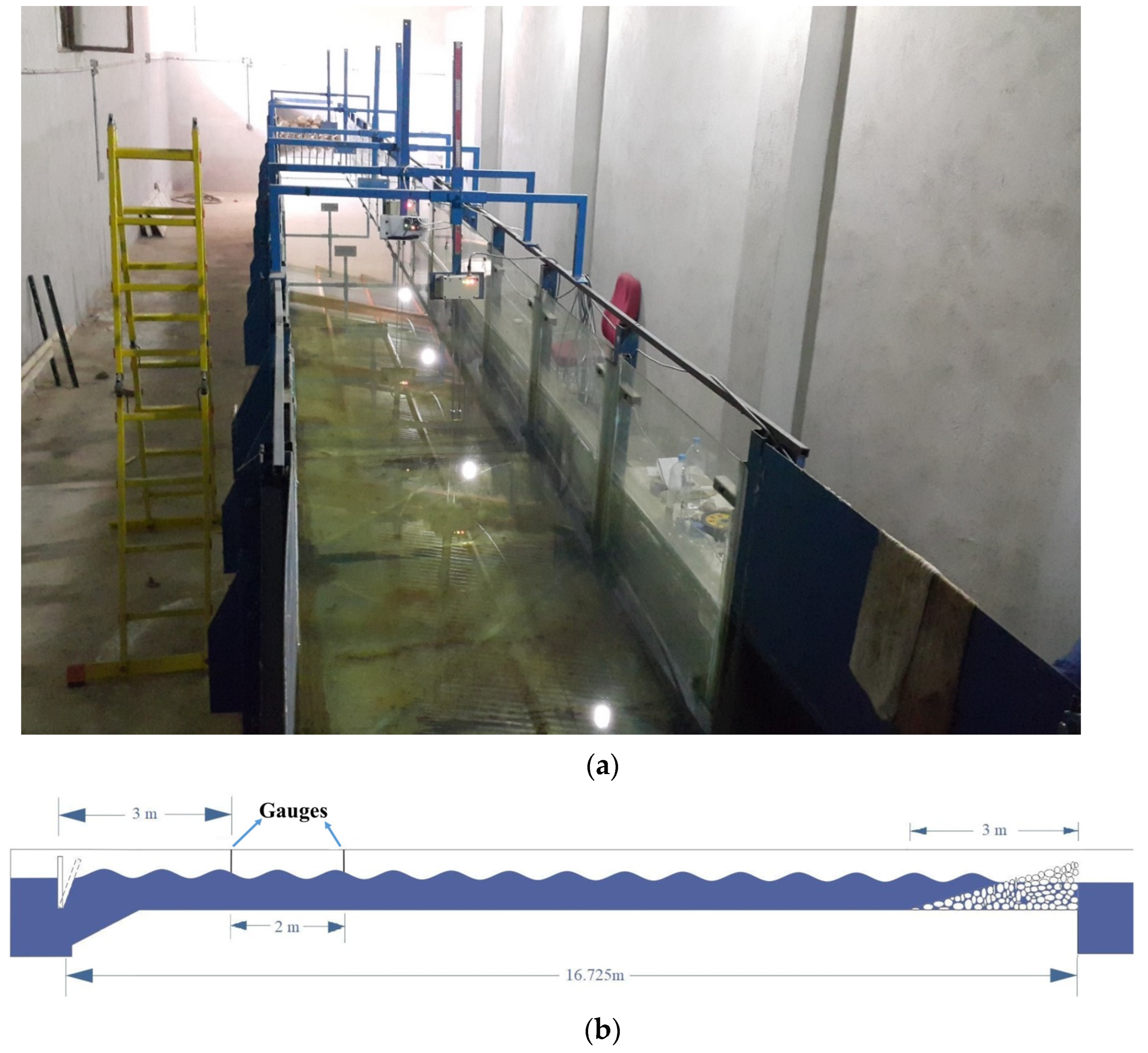
The experimental study of this research was carried out using a 16 m length flap-type wavemaker located at the laboratory at the Graduate University of Advanced Technology, Kerman. This wavemaker has a rectangular cross-section with 1.07 m height and 1.045 m width. Figure 1 shows an overview of the wavemaker tank in the laboratory.
2.1. Wave Generation
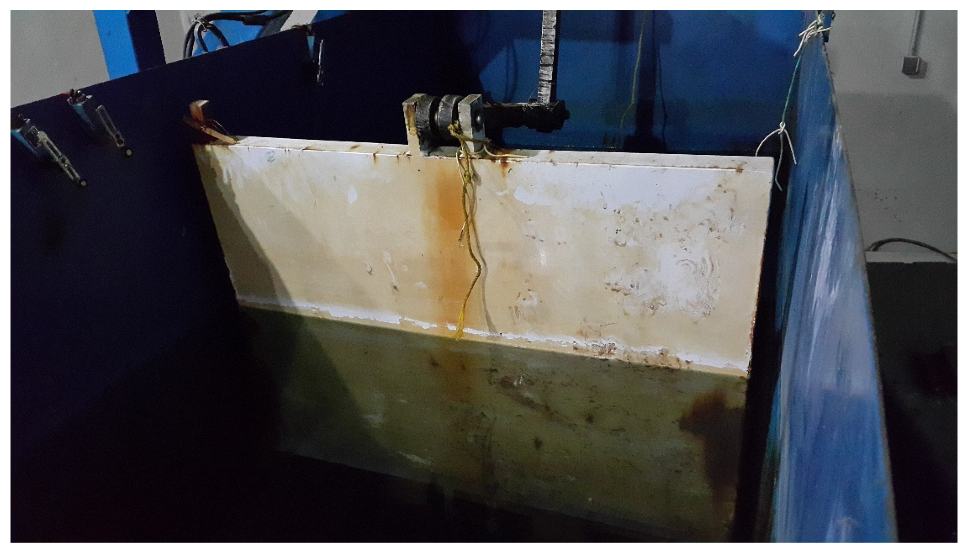
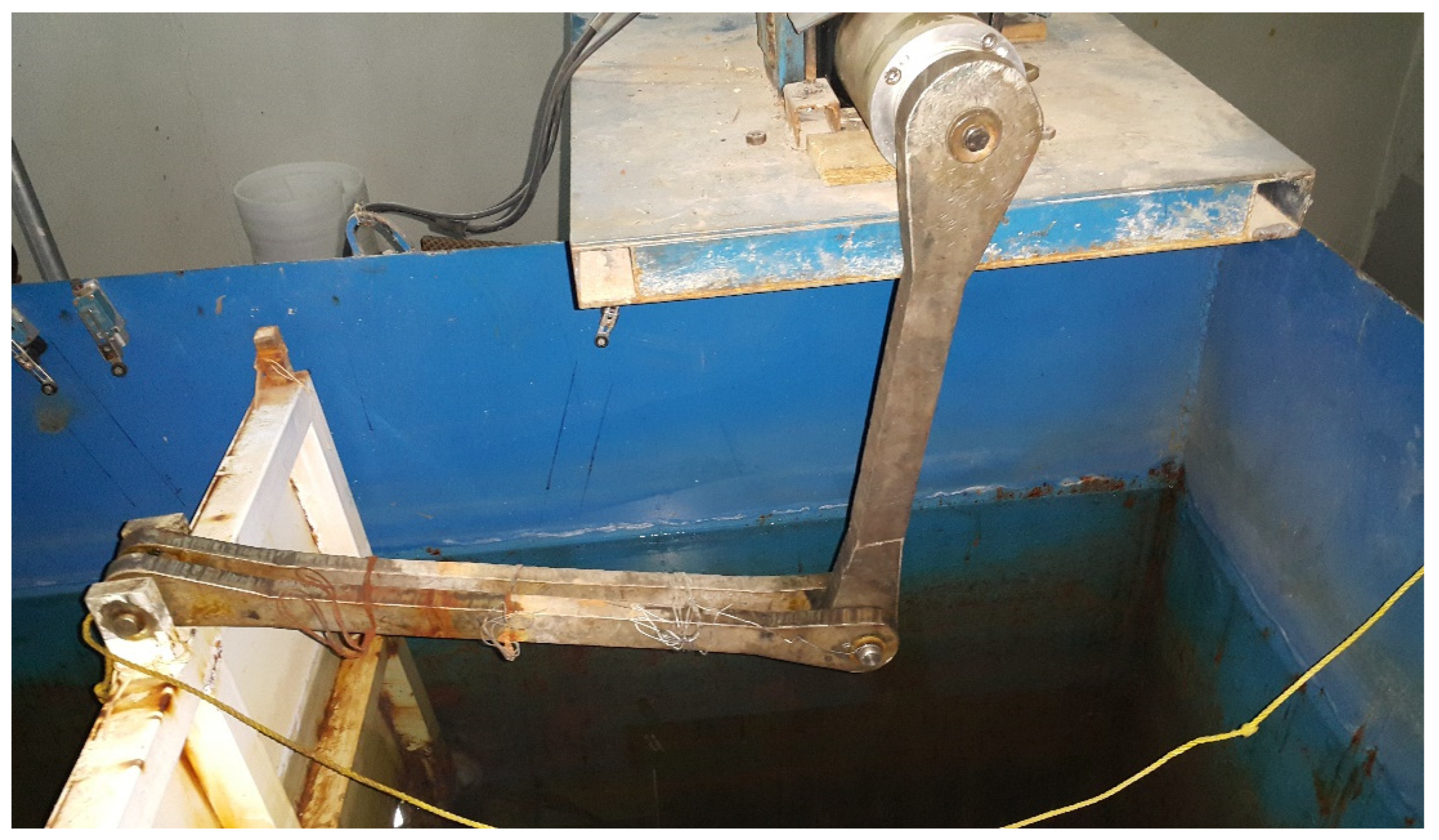
The generation of waves in the experimental wavemaker is carried out by a flap with 95 cm height, 96.5 cm width, and 5 cm thickness, which is hinged to the channel (Figure 2). As shown in Figure 3, the flap of the wavemaker is connected to a smart electric motor using two arms 65 cm and 50 cm long.
Generation of the waves is performed using the device software. The software produces a pulse using the data received from the operator, such as water depth, wave frequency, wave height, and wavelength. This pulse determines the amount of flap motion in a given time based on the frequency of the wave.
2.2. Wave Energy Dissipation
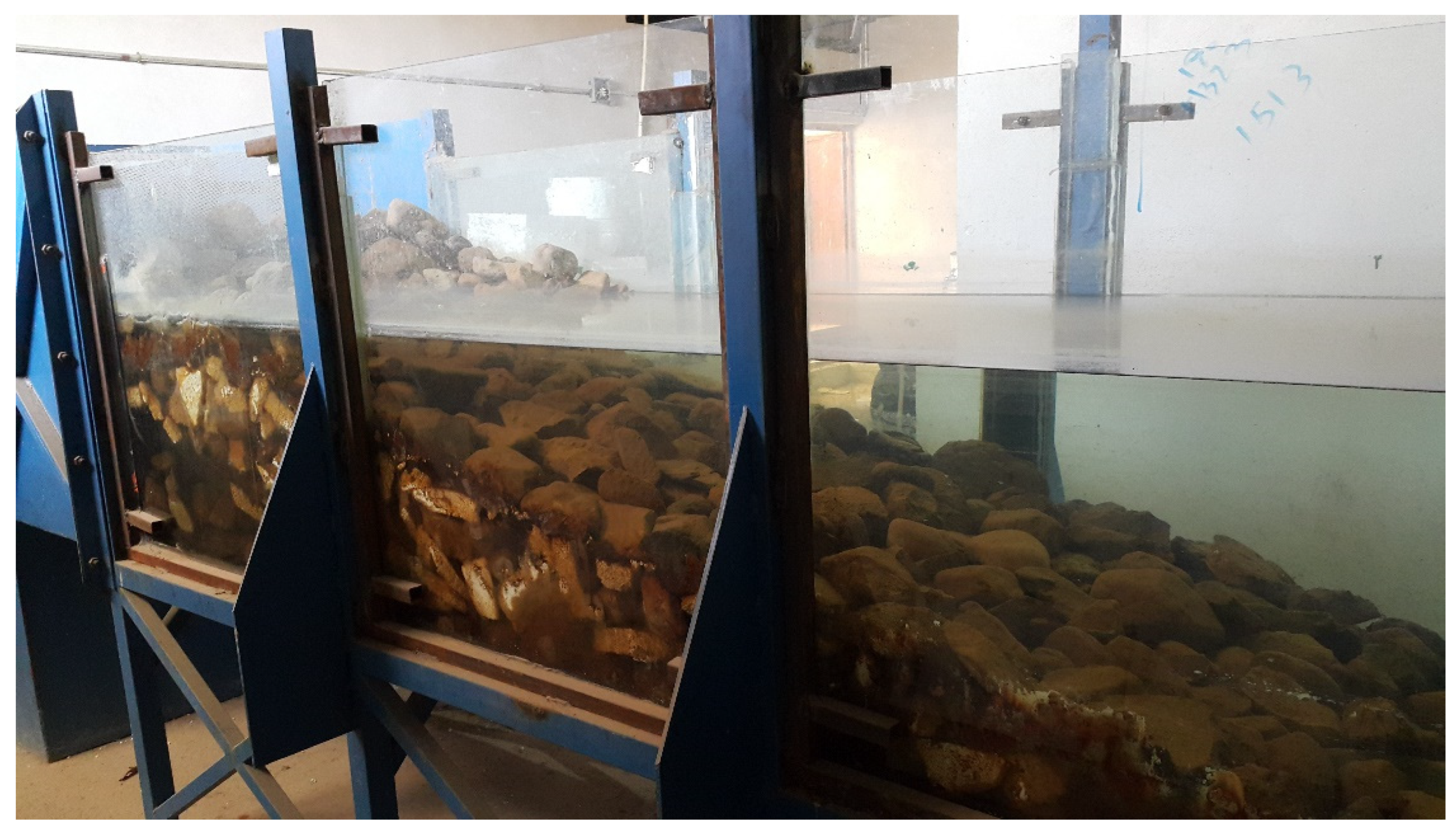
Because the wave tank is a rectangular cube with a closed end, a beach or wave absorb system is needed to dissipate or absorb the wave energy. For this purpose, an inclined stone beach was made at the end of the experimental wave tank (Figure 4). It should be mentioned that the free surface of the water becomes smooth after the collision with the beach in all experiments, which indicates the complete wave energy dissipation through the beach.
2.3. Wave Gauges
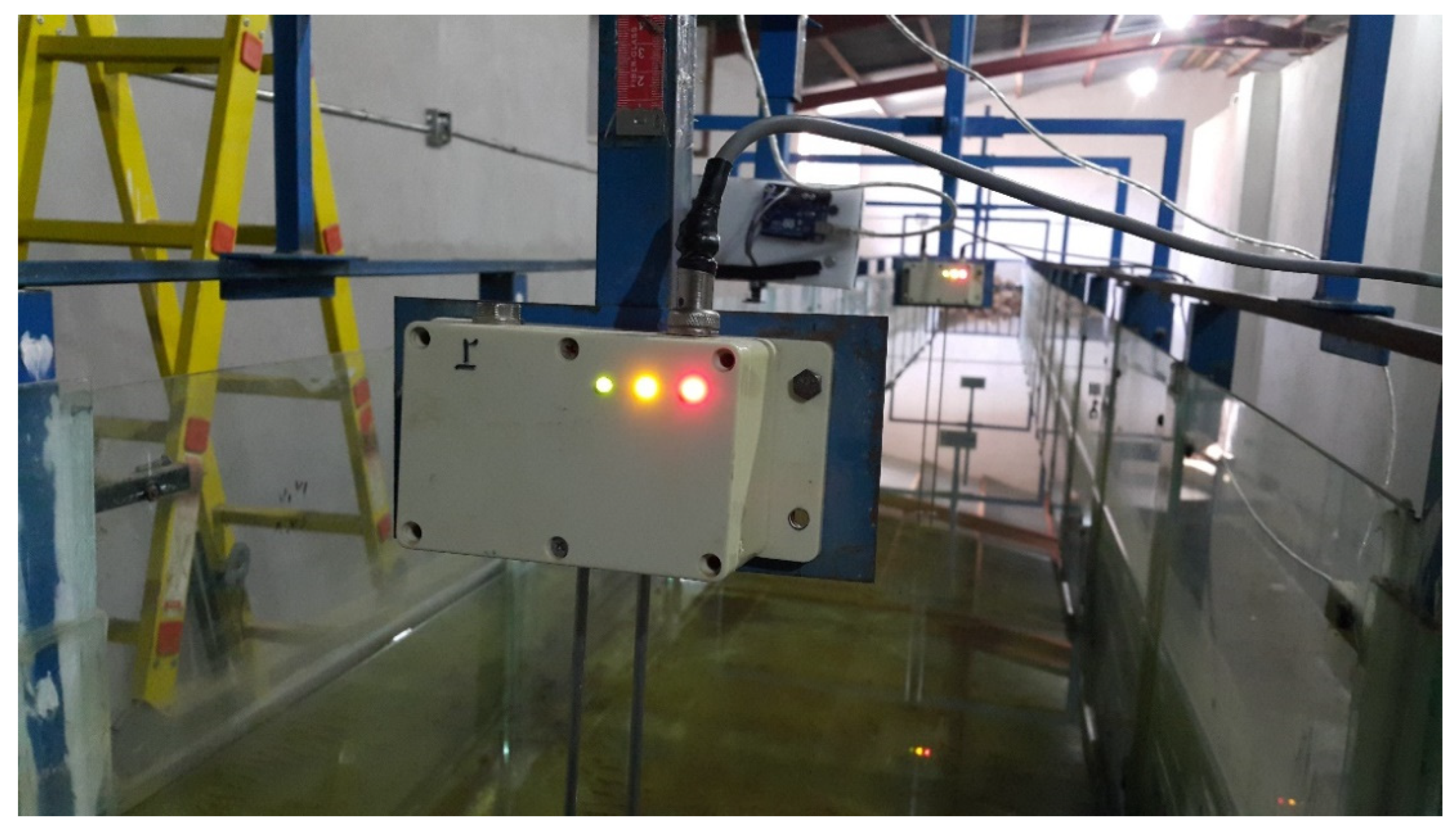
In the wavemaker tank, the resistance wave probe is used to measure wave height. As has been shown in Figure 5, the wave probe consists of two bars 50 cm in length and 0.5 mm in diameter. Sensors are located where the amount of water height is required and measure the surface water oscillation with a precision of millimeters. These instruments were connected in series with a 4-string cable, and the first probe was connected to the data logger of the wave tank.
3. Simulation Method
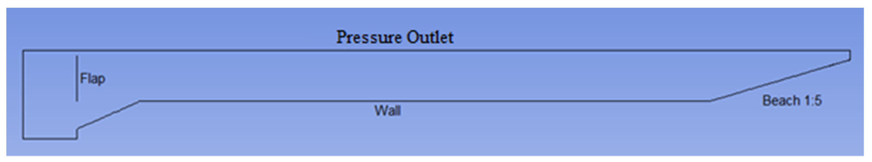
The numerical wave tank is simulated similarly to the available experimental wave tank in the laboratory. Real dimensions of the experimental wavemaker tank are used for numerical modeling in Fluent software. A schematic of the 2-D model of the wave tank is shown in Figure 6.
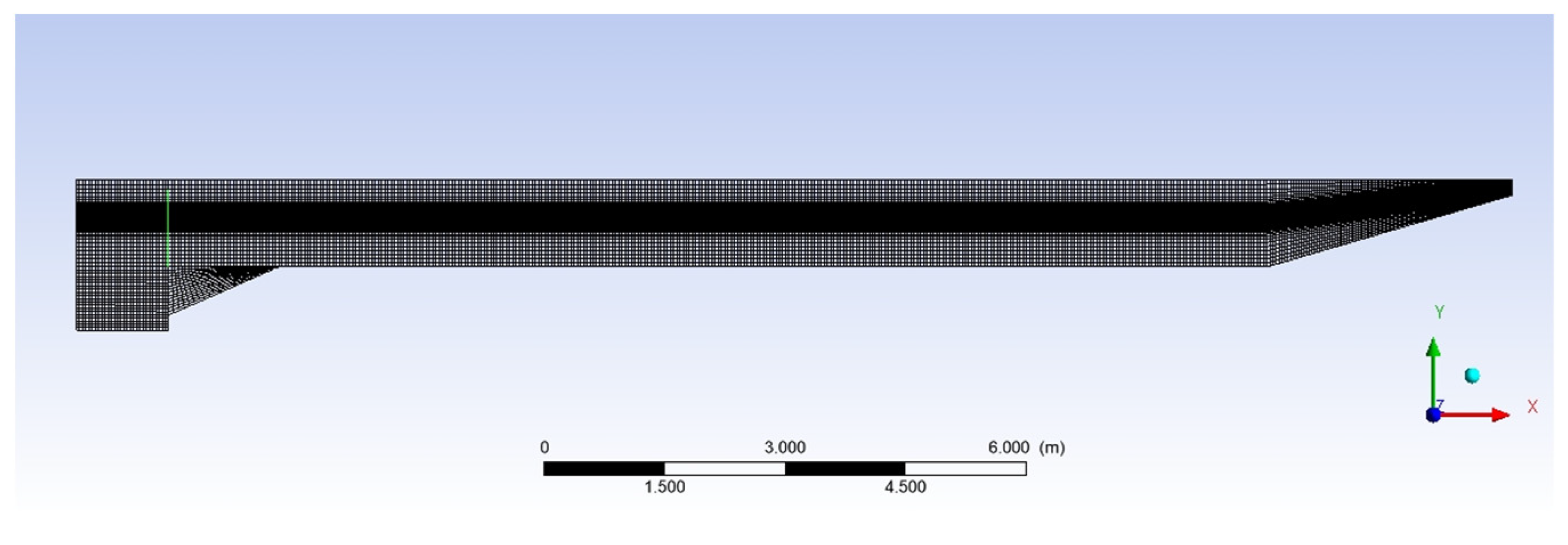
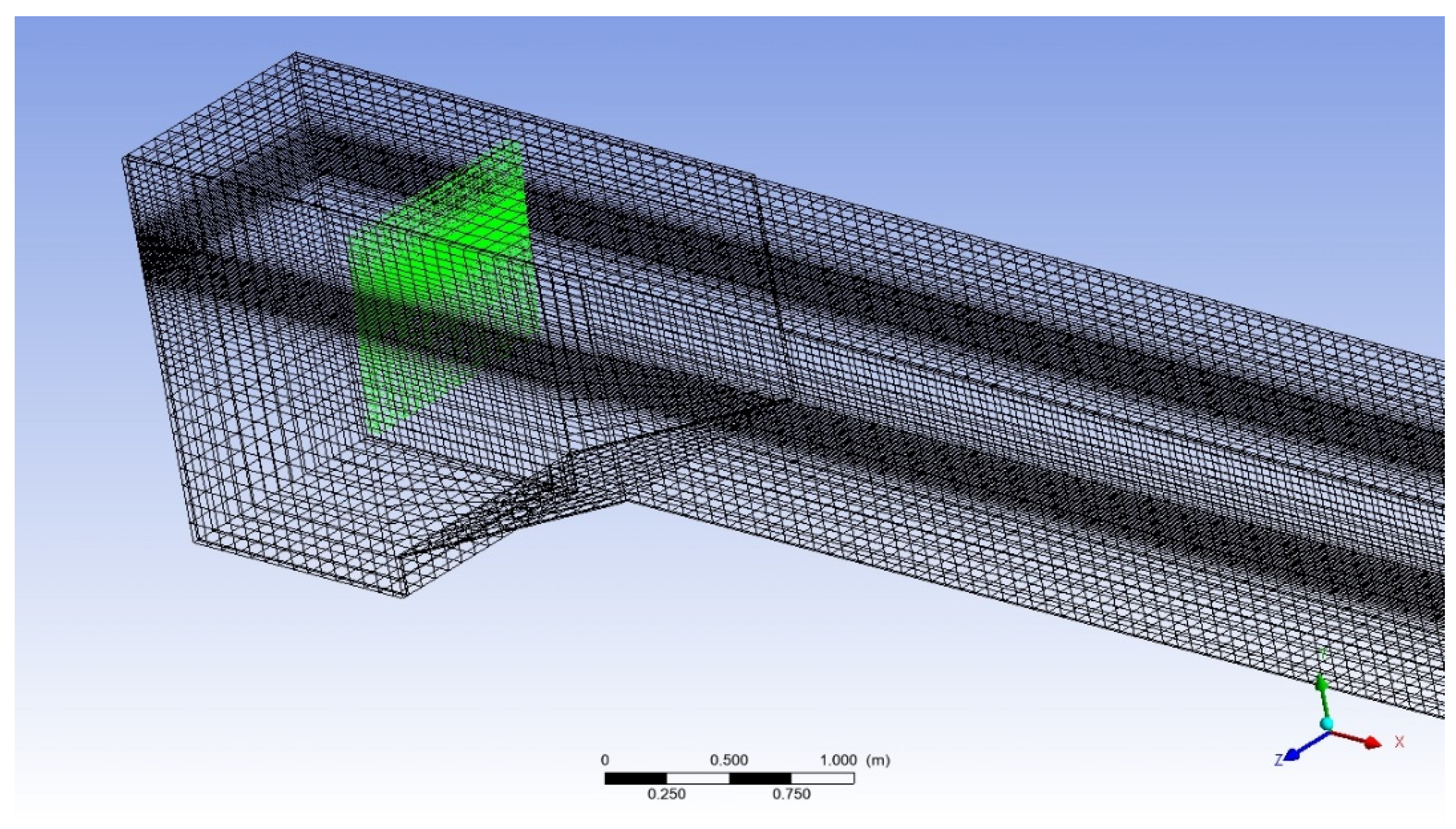
To accurately obtain the wave height, a fine mesh is used at the border of two fluid phases, i.e., water and air, in both two-dimensional and three-dimensional numerical-wave tanks. Samples of 2-D and 3-D mesh employed in the numerical simulation are shown in Figure 7 and Figure 8, respectively.
3.1. Governing Equations
The governing equations of this problem are the conservation of the mass and Navier–Stokes equations:
where is the velocity vector, t is the time, P is the pressure, is the stress tensor, is the gravitational acceleration vector, and is the volume force vector.
To determine the free surface elevation, the volume of fluid (VOF) method is used according to the following equation:
where F is liquid volume fraction. The amount of this parameter does not directly enter into the momentum equation, but it affects the viscosity and density of the fluids:
where the subscripts g and l represent gas and liquid phases, respectively.
3.2. Numerical Method
To simulate waves in the wave tank, all governing equations should be solved with the transient mode of Fluent software. The flow is laminar, and the multiphase model is activated using the VOF method. The boundary condition of the top boundary of the tank is selected for the flow of air; other boundaries are the wall with a 1:3 inclined beach (Figure 6).
Dynamic Mesh
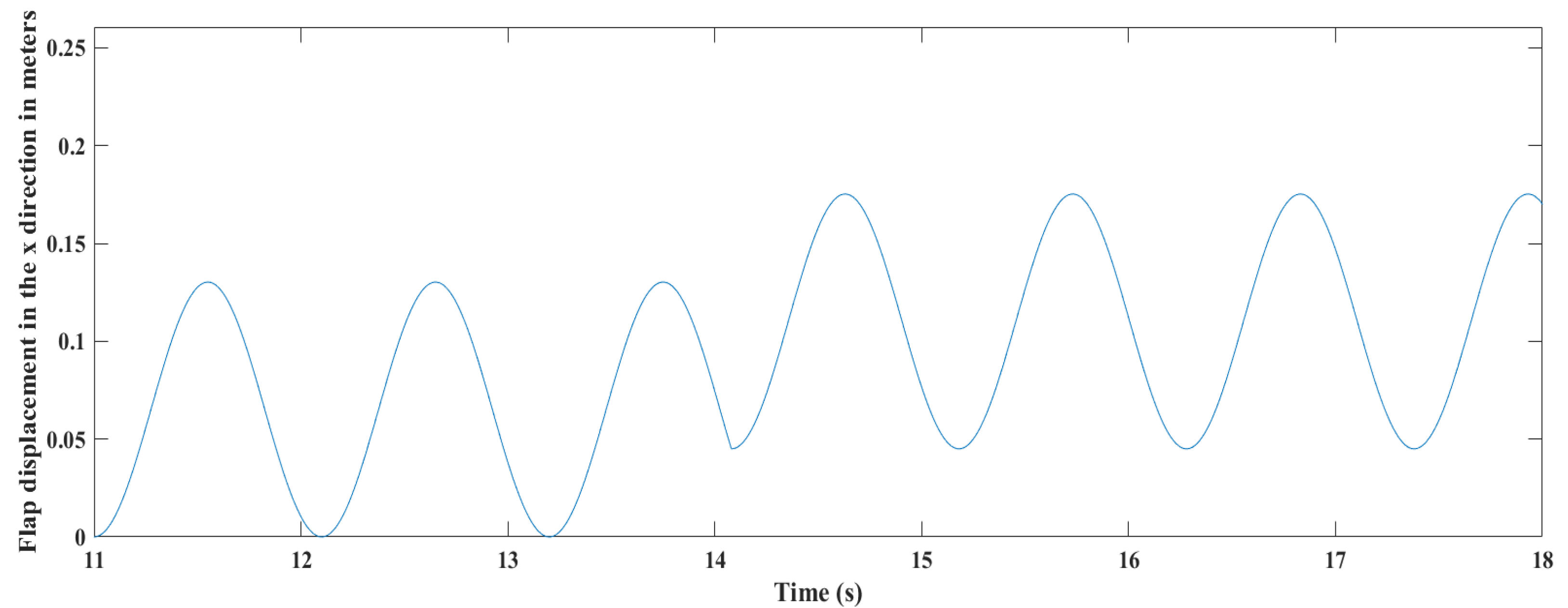
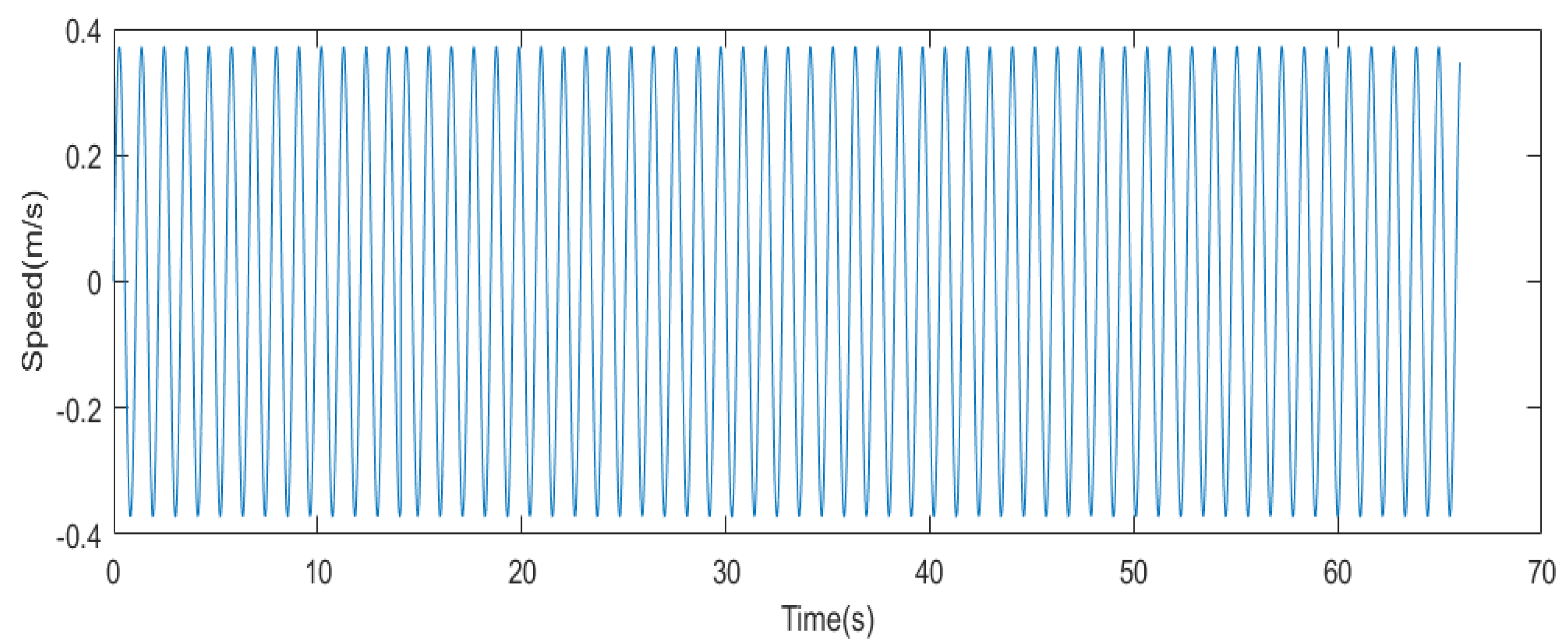
To fully simulate the flap movement of the laboratory wave tank, it is necessary to measure the displacement of the flap in each experiment. To measure the displacement of the flap, a meter was used along the x direction (length of the tank), and the amount of displacement was read with each rowing. After obtaining displacement, rowing motion was simulated using MATLAB software. To transfer flap motion to Fluent software, flap speed needs to be entered. It was derived from the flap motion equation in MATLAB software to obtain the flap speed, and then the flap speed obtained from MATLAB software was entered into Fluent. Figure 9 shows the flap movement in the x direction for each experiment, and Figure 10 shows the speed corresponding to it.
There is a problem in the engine of the laboratory tank such that, in all tests after 12 cycles and in the 13th cycle, the complete device does not return to its initial state and starts the next cycle at a certain interval in each test. This is shown in Figure 9 from about 14 s onwards. A dynamic mesh in Fluent software is used to model the movement of the flap, and the flap’s motion equation is applied using a user-defined function (UDF). As seen in Algorithm 1, examples of codes (Algorithm 1) written for flap in Fluent software were given.
| Algorithm 1 Computer programming codes provided for flap in Fluent software. |
| #include “udf.h” DEFINE_CG_MOTION (Case1, dt, vel, omega, time, dtime) { if (time < 14.0801) omega [2] = −0.3722 ∗ cos(5.7120 ∗ time−2 ∗ atan(1.0)); else if (time < 66) omega [2] = −0.3722 ∗ cos(5.7120 ∗ (time + 0.2199)−2 ∗ atan(1.0)); else omega [2] = 0; |
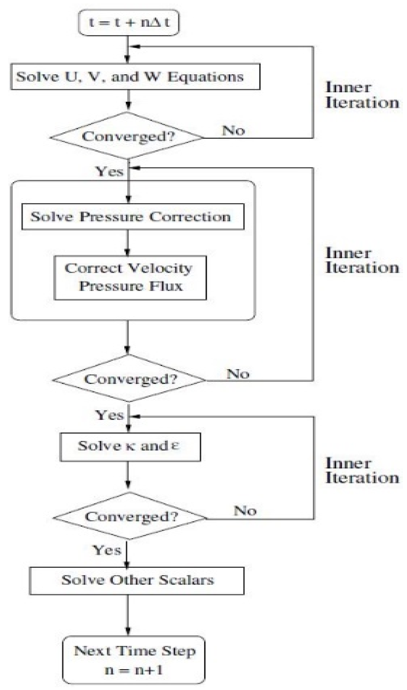
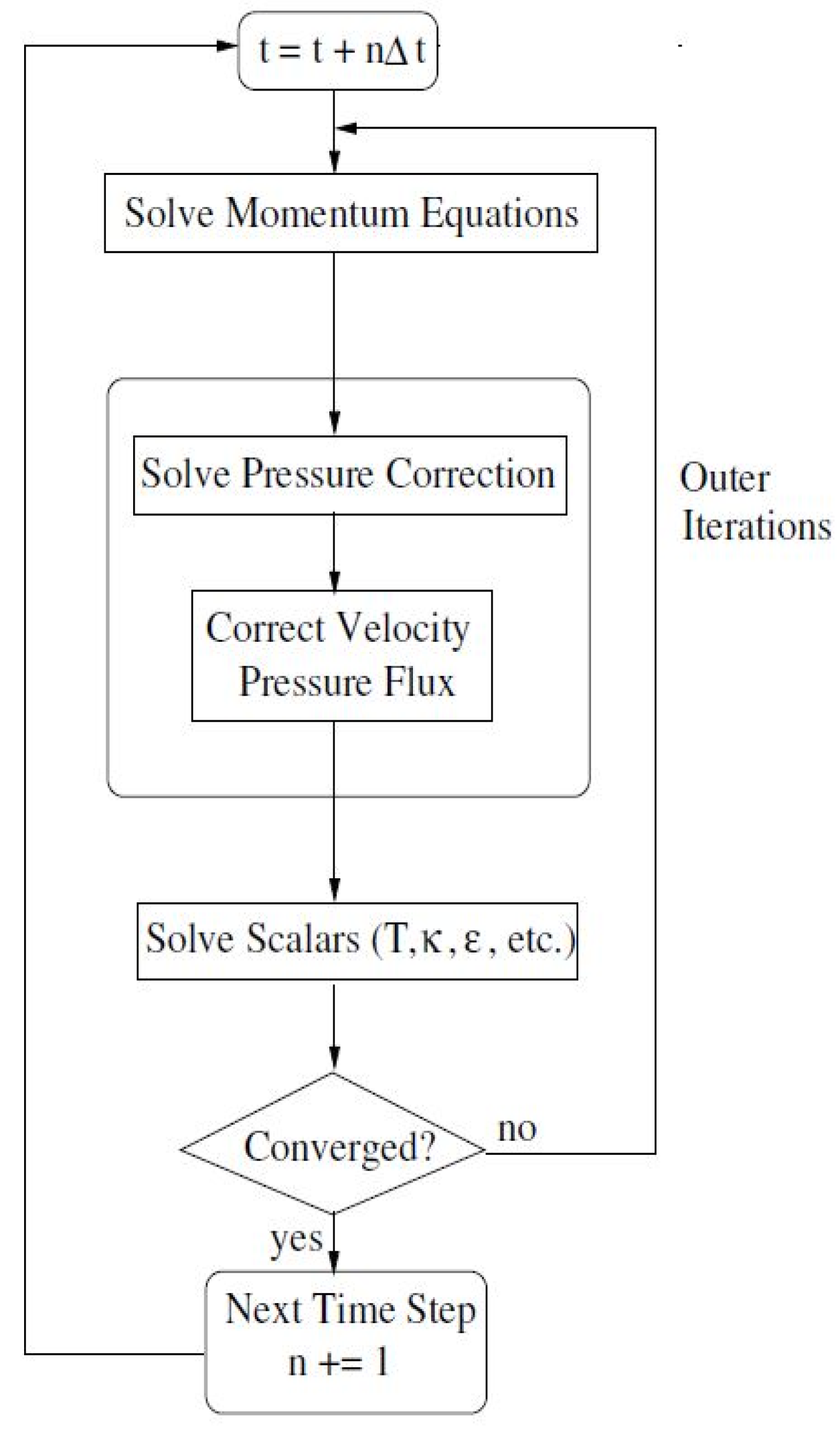
In unstable problems, there is a solution method called noniterative time advancement, which is used in this research. In this method, the solution time is much faster than that of the usual methods. The reason for this is that the outer iteration loop is faster. In Figure 11 and Figure 12, the solution method of this method is compared with a normal solver. The accuracy of this method is less than the default Fluent method, although it can be ignored due to its higher speed.
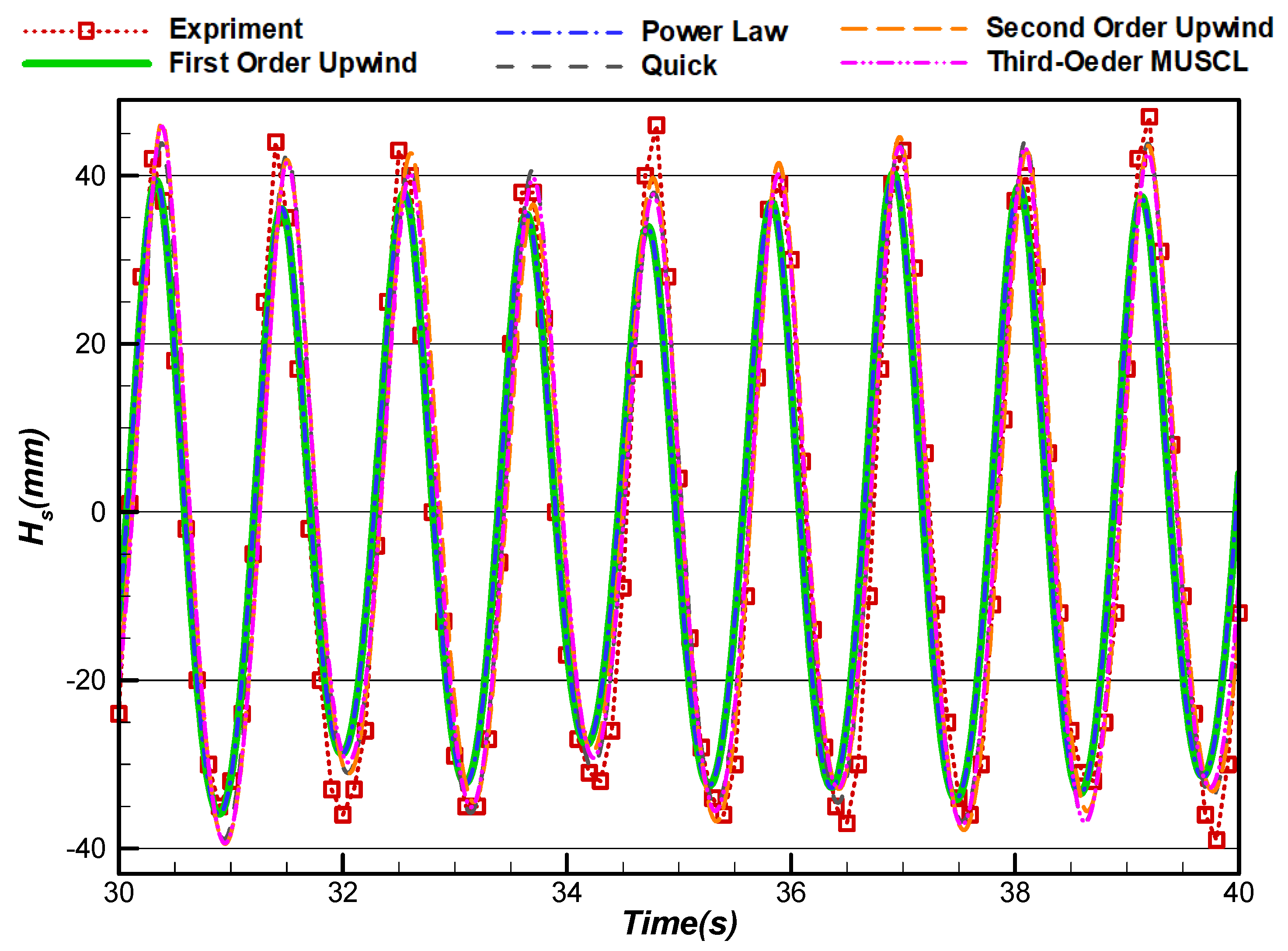
By using this method, the computational time becomes much faster than usual. Additionally, only two schemes exist in a transient mode in Fluent for the pressure–velocity coupling, named PISO and FSM algorithms, among which the PISO algorithm was selected in this work. For the spatial discretization of the momentum equation, different Fluent methods were used to model a sample wave, and the results were compared to find the best discretization scheme for the current work (Figure 13). As shown in Figure 9, since the results of the second-order upwind scheme were identical to higher schemes such as Quick and MUSCL schemes and this method was more stable and faster than the higher schemes, the second-order upwind scheme was used for the spatial discretization of the momentum equation.
4. Simulation Results and Discussions
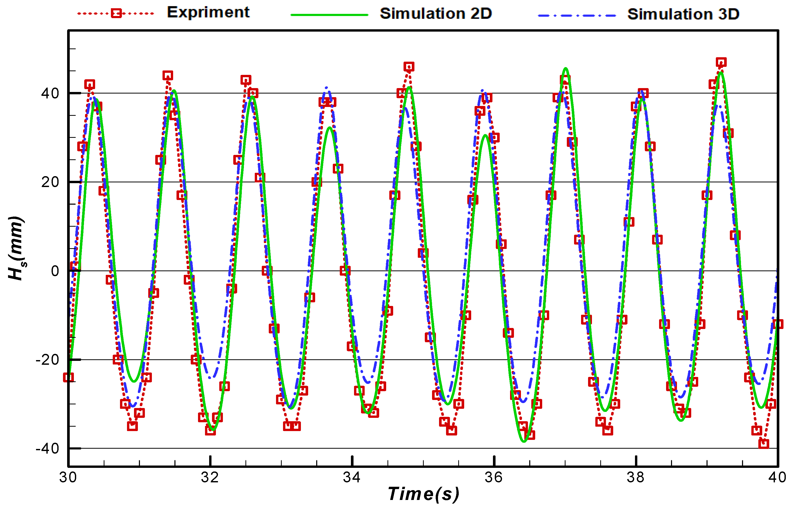
In many simulated problems, two-dimensional and three-dimensional results are similar to each other, and two-dimensional results are used to reduce computational costs. In this study, a three-dimensional wave tank was first analyzed, and then a two-dimensional wave tank was simulated. Two-dimensional, three-dimensional, and experimental results were compared for a sample case (Figure 14). The computational time of the 3-D problem was about 22 days using one CPU of an Intel Core 2 Quad operation machine (model name: i5-4400, number of CPUs: 4, CPU frequency: 3.1 GHz, and memory size: 16 GB), but for the 2-D one, it reached 9 h using the same computer. As can be seen from Figure 14, the comparison of the two-dimensional and three-dimensional results with the experimental ones shows that both numerical results are close to the experimental ones and that neither of them is superior to the other one. Therefore, to reduce the computational costs in this research, two-dimensional wave tank simulation was used for obtaining the results hereafter. It should be mentioned that the reason for the difference between 2-D and 3-D numerical simulations is that, in 3-D simulation, the entire wave tank is simulated with all actual details of the experimental wavemaker, and the effects of quantities and parameters in the z-direction such as the difference between the width of the flat paddle by the width of the tank impact the results.
4.1. Mesh Independence
To check the mesh independency in this research, the profile of the wave height was obtained to reach a mesh-independent solution. For this purpose, as previously shown in Figure 7 and Figure 8, a fine mesh is used for the area between the two phases (air and water).
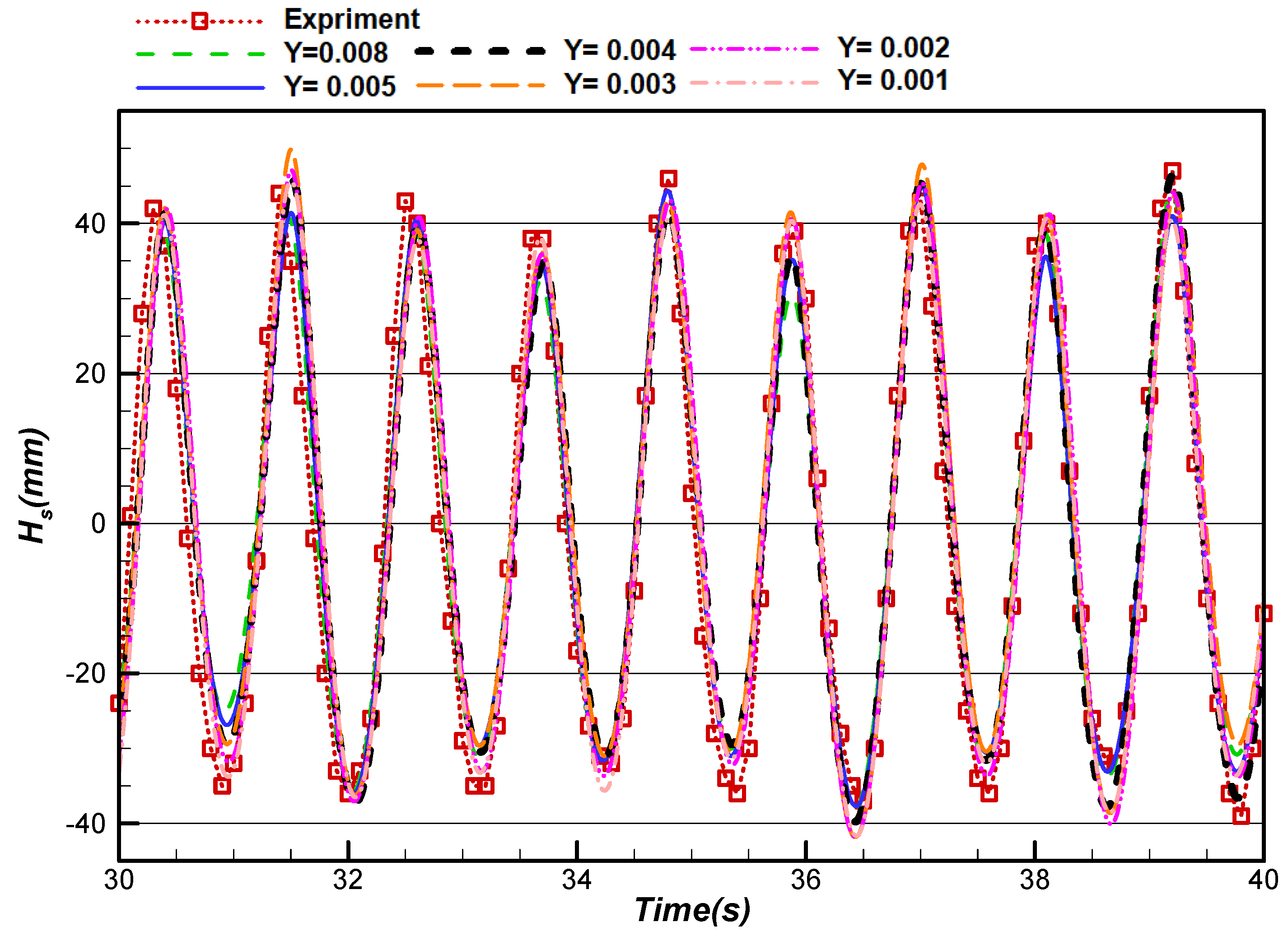
To maintain the quality of the mesh and to keep the maximum aspect ratio of the grids below 20, by reducing the mesh height of the cells at the common boundary of two fluids, the length of the cells should also reduce. Different mesh sizes are used to check the mesh independence of the numerical simulation as shown in Figure 15. In Figure 15, Y is the height of the cells in meters at the common boundary of two phases, and experimental results are also shown to validate the numerical results.
As seen in Figure 15, the results of a cell height below 5 mm are similar to . Therefore, reducing the cell size to below 5 mm does not change the results but increases the computational cost by increasing the number of meshes. The cell number of different meshes produced for different cell heights is shown in Table 1, and the number of meshes of 37,686 for is chosen for the simulation carried out in this study.
4.2. Model Validation
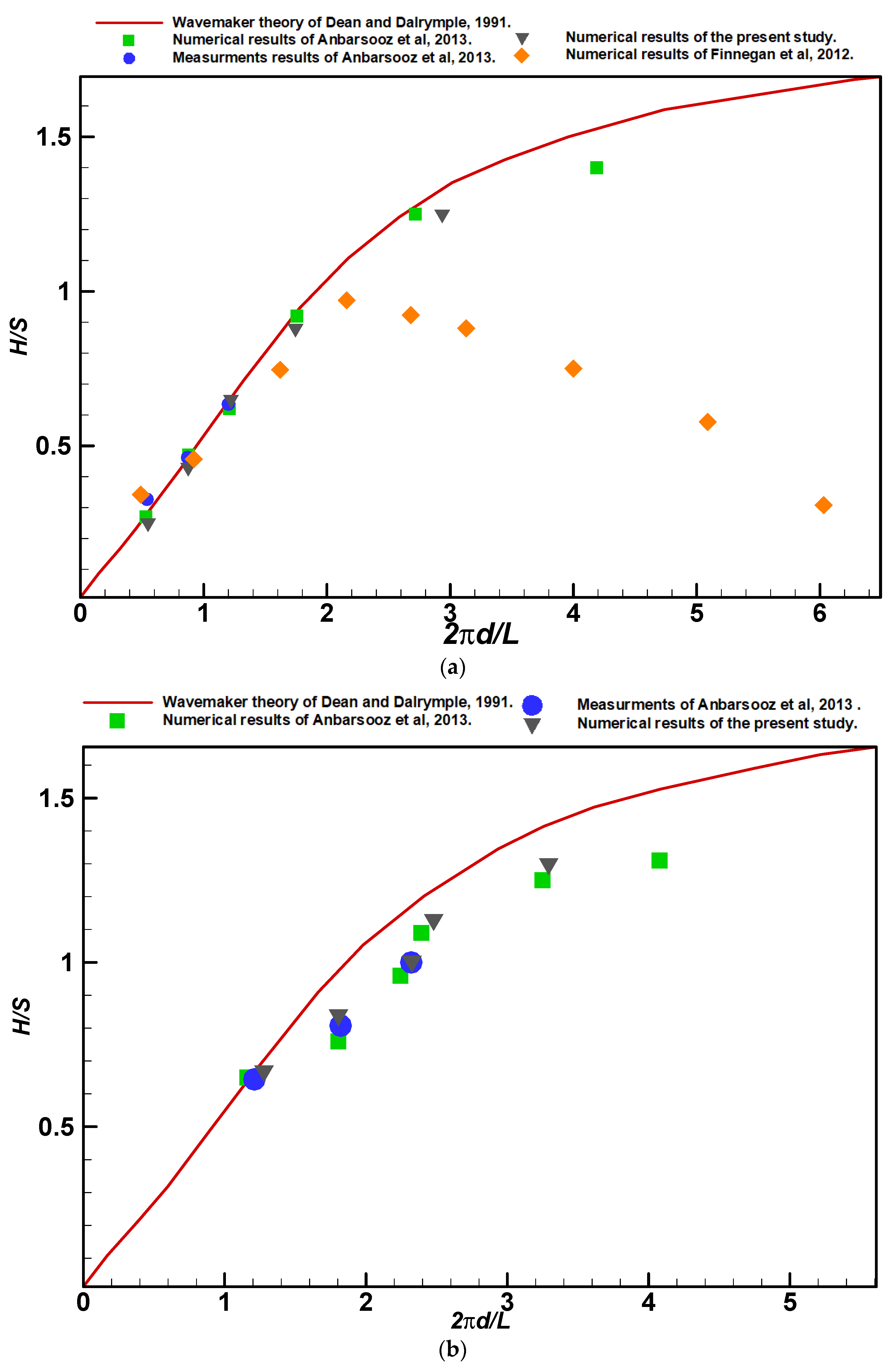
In this work, to validate the numerical wave tank at different frequencies, wave heights, and water depths, the experimental, numerical, and theoretical results of other researchers are used. Different waves generated in the present numerical wave tank are compared with the analytical results of Dean and Dalrymple [30] as well as the numerical and empirical results of Anbarsooz et al. [4] and the numerical results of Finnegan and Goggins [22].
To generate the desired waves, the motion and velocity of the flap should be simulated like the other studies using the following formulas [4]:
where S is the flap’s location along the horizon, is the range of flap angles, d is the depth of water, T is the time period, and θ is the angular velocity of the flap.
The waves generated are divided into two categories: (i) small wave steepness with an H/L ratio (H: wave height and L: wavelength) between 0.02 and 0.03 and (ii) high wave steepness in which the H/L ratio varies from 0.044 to 0.048. Table 2 shows the results of the generated waves for the validation process.
In Figure 16, the comparison of the results obtained from the waves generated in this study with the analytical, numerical, and experimental results of other researchers is observed. By comparing the results obtained from the numerical wave tank developed in this research and other studies, the accuracy of the results can be found.
4.3. Wave Generation Results
Five different waves with the specifications shown in Table 2 are generated in the experimental wave tank, and the height of the waves is measured by using the wave probe at distances of 3 and 5 m from the flap. In Table 3, Hs represents the wave height in millimeters, which is given to the device software, and H is the depth of water from the beginning of the flap. These cases are chosen to investigate the effect of different wave heights (Hs) and frequencies of the waves on the experimental and numerical simulation results.
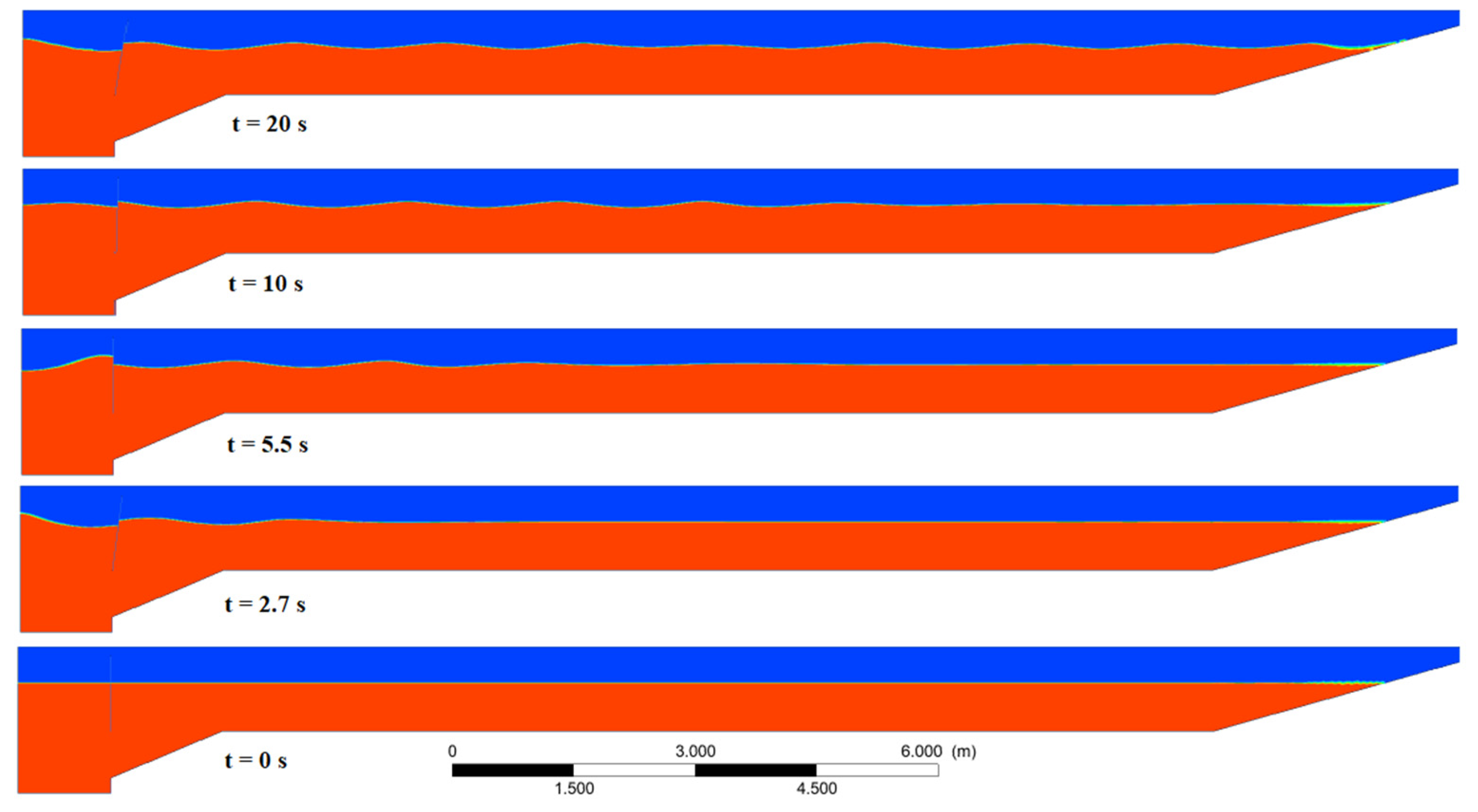
The waveform and the movement of the flap paddle in the numerical wave simulator are shown in Figure 17 at different times. As can be seen, with the passing of time, the waves are gradually created and moved from the tank to the beach slope.
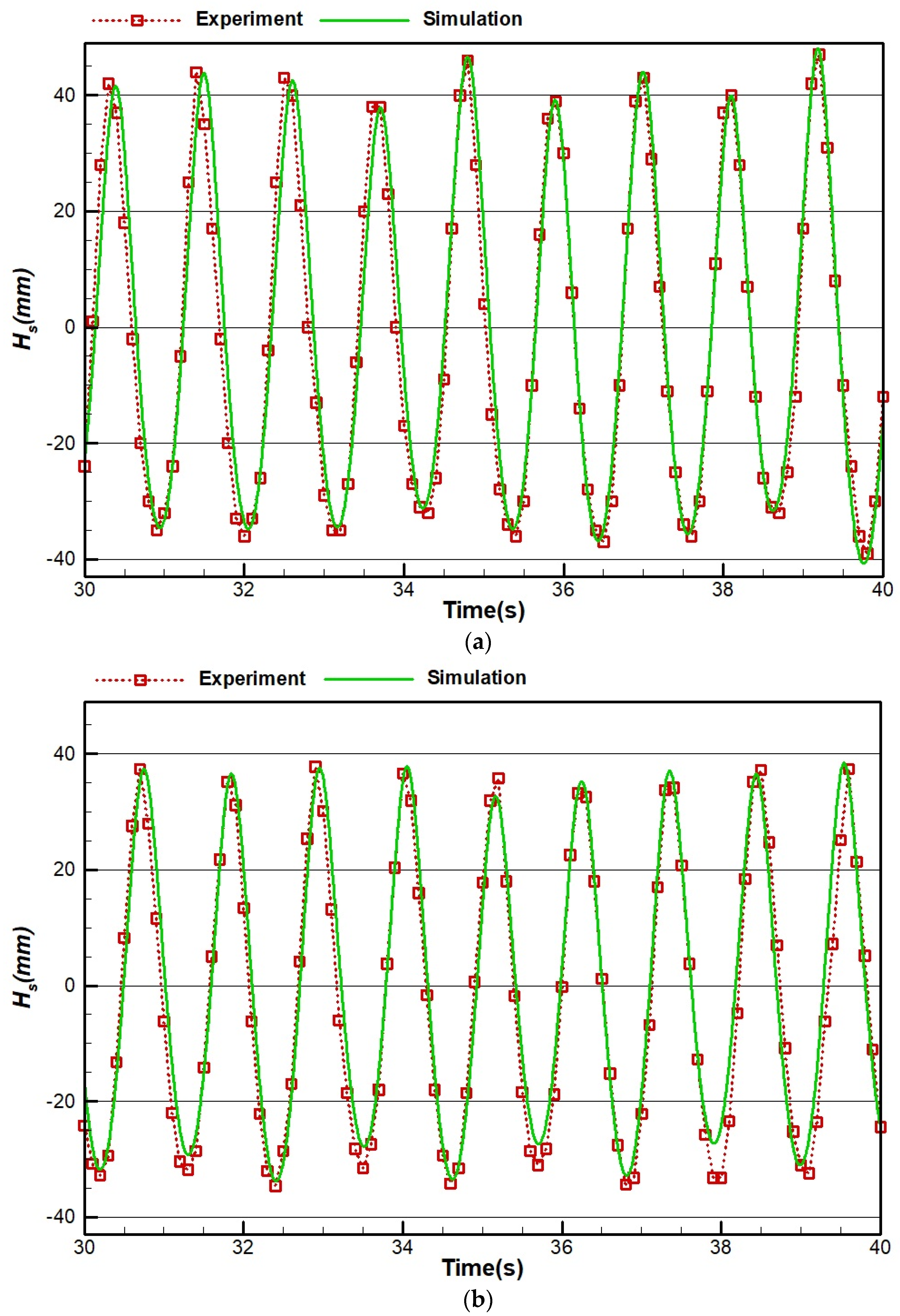
The results of experimental and numerical simulation for the waves are summarized, shown, and compared in Table 2. For each case, the height of the wave is plotted in a period of 30 to 40 s for the distances of 3 and 5 m of the flap.
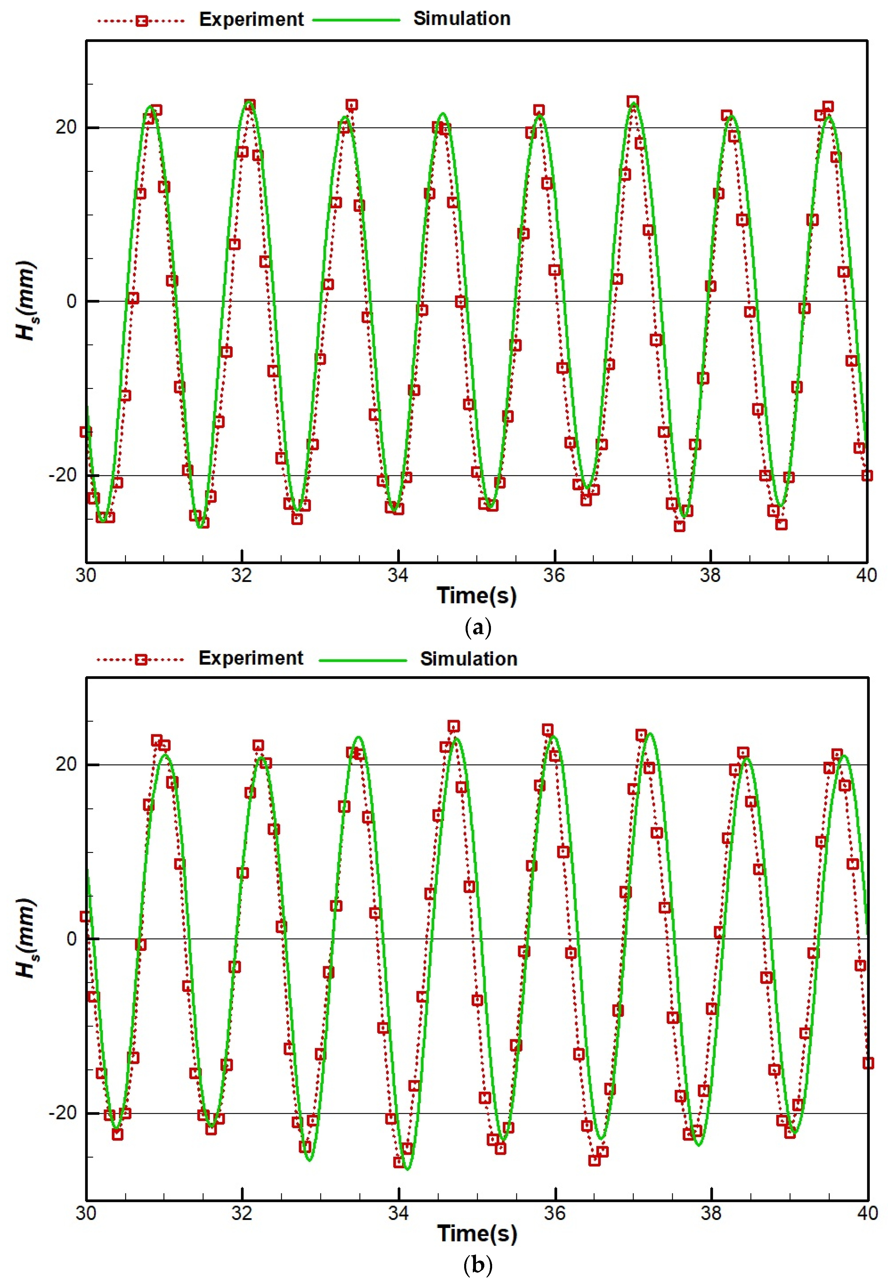
Figure 18 shows the results of case 1 for both experimental and numerical simulation. As demonstrated in Figure 18a,b, the numerical wave tank could properly simulate the experimentally generated wave. However, the accuracy has been reduced for the results at the distance of 5 m from the flap, and sometimes, the numerical results overshoot or undershoot the experimental results.
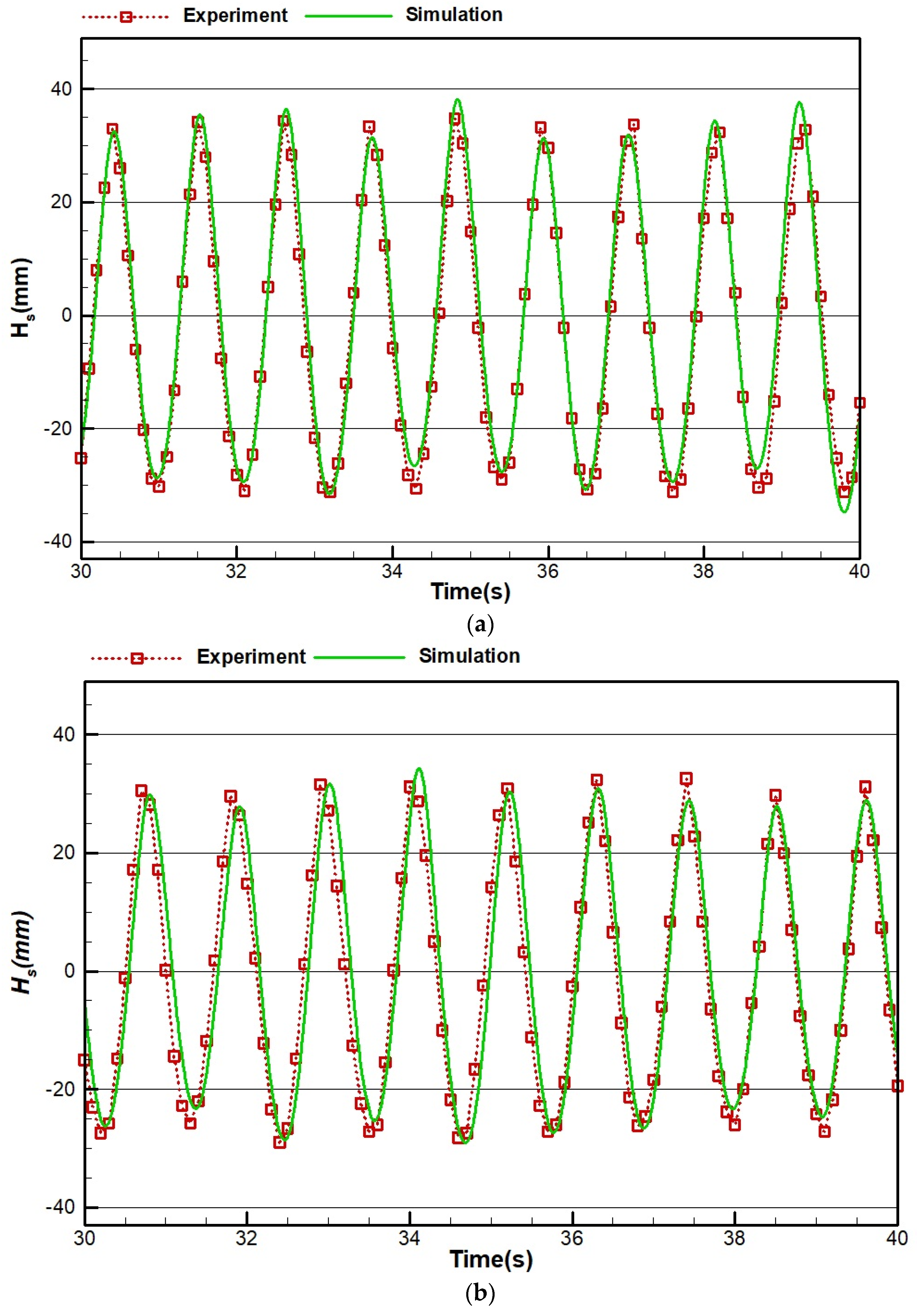
Figure 19 shows the results of the wave simulation of case 2 at distances of 3 and 5 m from the flap. According to Table 2, the wave specifications of this case are like case 1 except that Hs is reduced from 50 mm to 30 mm. Similar to case 1, it is seen that the numerical wave tank could simulate the wave of case 2, although the precision of the numerical simulation has been slightly reduced in this case rather than in case 1.
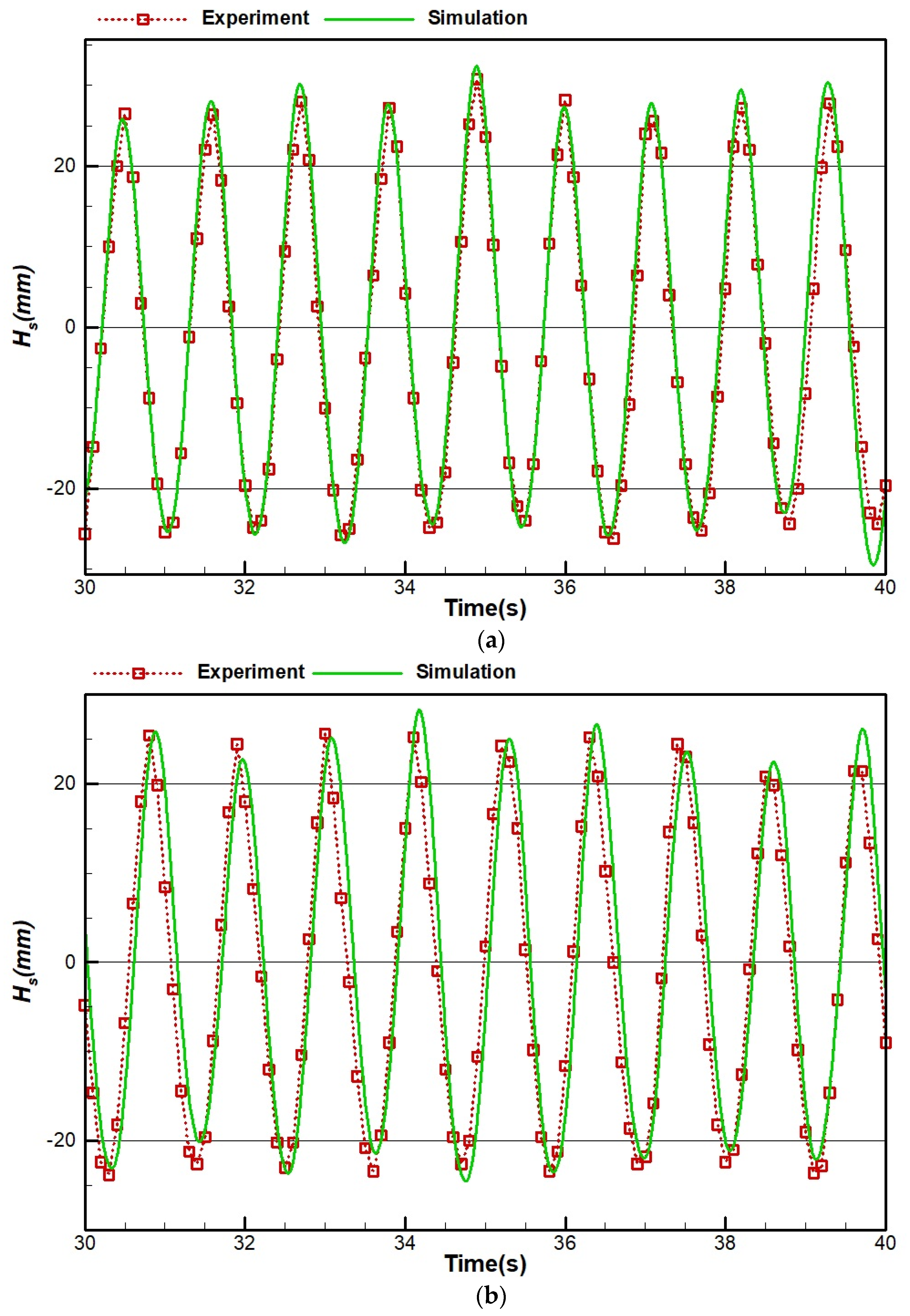
The results of the wave generated from case 3 are shown in Figure 20. As expressed in Table 2, the Hs of the wave, in this case, is reduced more than in the previous cases to 20 mm. Figure 20 illustrates that the discrepancy between the numerically simulated results and the experimental ones has increased compared with cases 1 and 2. From Figure 19 and Figure 20, it can be concluded that the accuracy of the simulation wave is reduced by decreasing the height of the wave.
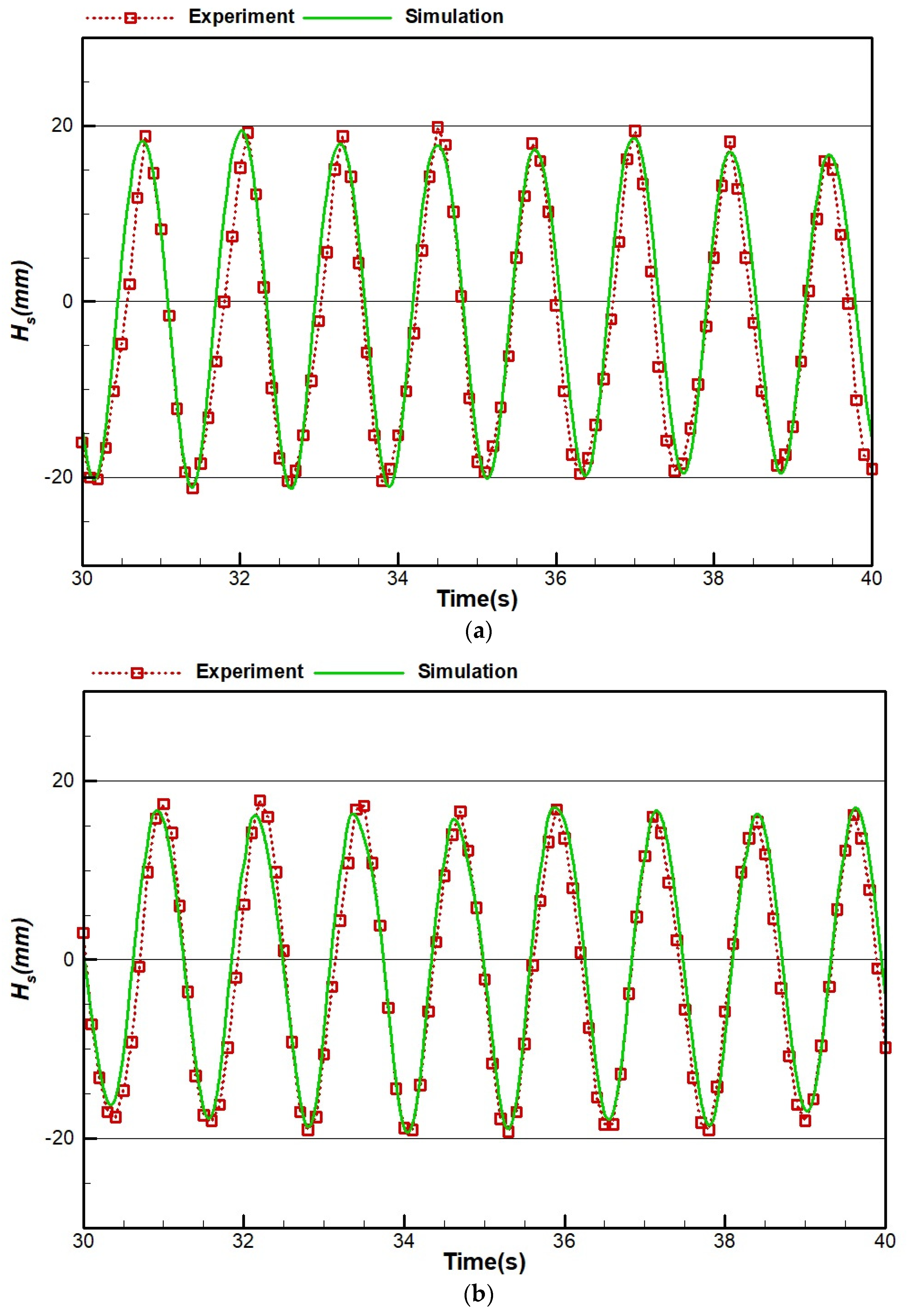
Figure 21 illustrates the numerical and experimental results of the wave of case 4. The specifications of this wave are like case 2 but with increased frequency. Growth in the frequency means an increase in the speed of the wavemaker’s motor and the movement of the flap. Comparison of the results in Figure 19 and Figure 21 shows that by increasing the frequency of the wave, the numerical results are in good agreement with the experimental ones, and the difference between them greatly increased at a distance of 5 m.
Figure 18 shows the results of the wave of the last case (case 5). According to Table 2, this wave is like case 4 but with lower Hs or it is like case 3 but with higher frequency. A comparison of Figure 22 with previous results shows that there is a high discrepancy between the numerical and experimental results of this case, and especially at a distance of 5 m, this difference becomes very large. The reason as can be seen in the next part is the coast slope of 1:3. When the wave is not completely dampened, the reflected waves fall into the numerical wave tank and cause a disturbance in the waves. This disturbance is lower at a distance of 3 m from the flap because the reflected waves need more time to reach the distance of 3 m from the flap, while it is large at a distance of 5 m from the flap (Figure 22).
4.4. Study of the Beach Slope
In the experimental wave tank, to dissipate the energy of the wave and to prevent reversing the wave, a 1:3 triangular coastal beach composed of stones is used (Figure 4). These stones operate like a porous medium and dampen all the collisions to the beach. The simulated beach, as shown in Figure 6, is a simple wall with a 1:3 slope. This beach cannot completely dissipate the energy of the waves that hit it, and the reflected waves cause a numerical error in the simulation. To find a solution to this problem, other beach slopes, such as 1:4, 1:5, and 1:6, have also been simulated and compared to each other and the experimental results.
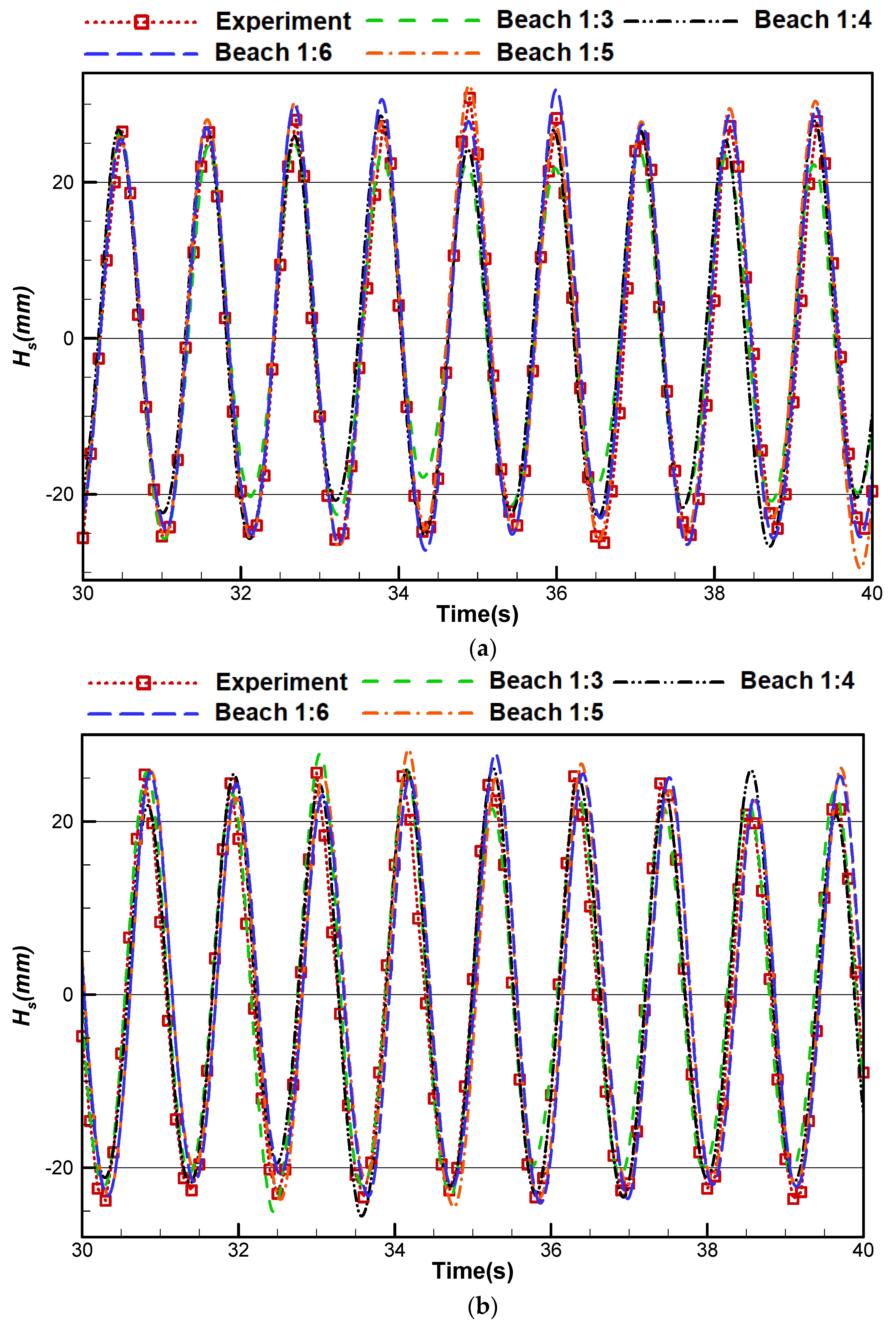
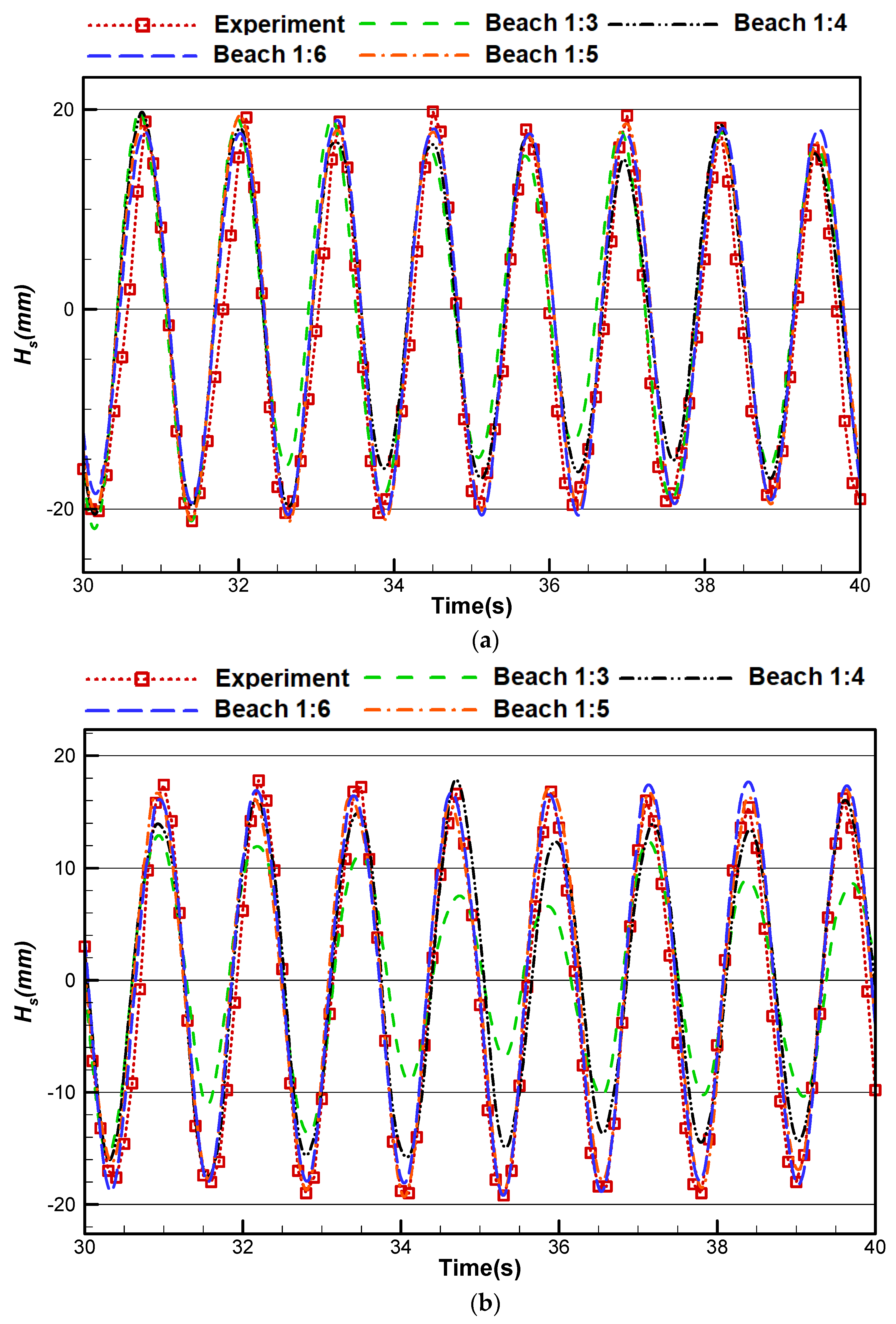
To perceive the effects of different beach slopes on the waves, Figure 19 and Figure 20 depict the results of the wave height of two wave cases, 3 and 5 (according to Table 2), for various beach slopes at distances of 3 and 5 m from the flap.
As shown in Figure 23 and Figure 24, slopes 1:5 and 1:6 have been able to dampen the waves well and prevent wave reflection, which causes an increase in the accuracy of the simulation with respect to the generated experimental waves.
In order to better understand the comparison of the different coastal slopes, the following equation is used [31]:
where is the wave reflection coefficient and and are the height of the largest and smallest produced wave at a point that is affected by the wave reflection, respectively. The results of different coastal slopes are shown in Figure 25.
According to Figure 25, it can be concluded that the 1:4 and 1:3 slopes cannot dampen the wave after a collision with the coast, and the reflected waves disturb the waves. For 1:5 and 1:6 slopes, the wave reflection coefficient is lower than that of other slopes, which indicates the damping of different waves in these slopes. By comparing the results of 1:5 and 1:6 slopes, it can be concluded that each of these slopes gives better results in some kinds of waves; for example, the 1:5 slope could damp the wave reflection for the 1, 3, and 4 wave cases, and the 1:6 slope had better results for the wave cases of 2 and 5. In general, the optimum slope in the present numerical wave tank was chosen to be the 1:5 slope due to the better damping of wave reflection and also due to the decrease in the geometry and mesh, resulting in a reduction in computational costs.
5. Conclusions
In this paper, the experimental analysis and numerical simulation of wave generations in a flap wavemaker tank were investigated and compared. The experimental results were obtained using the wavemaker, and additionally, the numerical simulation was performed by using Fluent software. To do this, first, different waves were generated in the laboratory wave tank, and the wave height was collected using wave probes at different distances from the flap. Then, these waves were numerically simulated. The effects of the height and frequency of the waves were examined by comparing the numerical simulation with the experimental results. Additionally, to find a proper slope of the beach at the end of the wave tank in the numerical simulation, different beach slopes were simulated, and their results were compared with the experimental ones.
From the results of this research, it was concluded that, to reduce the computational cost of the calculations, it was possible to use a two-dimensional numerical wave tank instead of the 3-D model. According to the results, it was seen that the numerically simulated wave tank in this research can properly simulate the experimentally generated waves, while the computational time of the present simulation is lower than the methods in the literature. The accuracy of the simulation slightly decreases by decreasing wave height and increasing frequency. From the survey of different beach slopes, it was derived that a 1:3 slope in the numerical simulation had the ability to dampen the energy of some waves (such as cases 1 and 2), but the best beach slope to absorb the energy of various kinds of waves was the 1:5 slope.
Author Contributions
Conceptualization, R.Z., K.L. and M.N.; Methodology, R.Z. and K.L.; Software, R.Z. and K.L.; Validation, R.Z.; Formal Analysis, R.Z. and M.N.; Investigation, R.Z. and M.N.; Writing—Original Draft Preparation, R.Z. and M.N.; Writing—Review and Editing, R.Z. and M.N.; Visualization, R.Z. and M.N.; Supervision, R.Z. and M.N. All authors have read and agreed to the published version of the manuscript.
Funding
This research received no external funding.
Institutional Review Board Statement
Not applicable.
Informed Consent Statement
Not applicable.
Data Availability Statement
Not applicable.
Acknowledgments
Authors greatly appreciate the Graduate University of Advanced Technology (Kerman, Iran) for providing experimental facilities.
Conflicts of Interest
The authors declare no conflict of interest.
References
- Amanatidis, G. European Policies on Climate and Energy towards 2020, 2030 and 2050. Policy Department for Economic, Scientific and Quality of Life Policies. European Parliament. 2019. PE 631.047. Available online: https://policycommons.net/artifacts/1335288/european-policies-on-climate-and-energy-towards-2020-2030-and-2050/1941726/ (accessed on 29 December 2022).
- Pecher, A.; Kofoed, J.P. Handbook of Ocean Wave Energy, 1st ed.; Springer: Berlin/Heidelberg, Germany, 2017. [Google Scholar]
- Lal, A.; Elangovan, M. CFD Simulation and Validation of Flap Type Wave-Maker. Int. J. Math. Comput. Sci. 2008, 2, 708–714. [Google Scholar]
- Anbarsooz, M.; Passandideh-Fard, M.; Moghiman, M. Fully nonlinear viscous wave generation in numerical wave tanks. Ocean Eng. 2013, 59, 73–85. [Google Scholar] [CrossRef]
- Han, Z.; Liu, Z.; Shi, H. Numerical study on overtopping performance of a multi-level breakwater for wave energy conversion. Ocean Eng. 2008, 150, 94–101. [Google Scholar] [CrossRef]
- Collins, K.M.; Stripling, S.; Simmonds, D.J.; Greaves, D.M. Quantitative metrics for evaluation of wave fields in basins. Ocean Eng. 2018, 169, 300–314. [Google Scholar] [CrossRef] [Green Version]
- Alamian, R.; Shafaghat, R.; Ketabdari, M.J. Wave simulation in a numerical wave tank using BEM. Am. Inst. Phys. Conf. Proc. 1648, 2015, 770008. [Google Scholar]
- Wu, Y.T.; Hsiao, S.C. Generation of stable and accurate solitary waves in a viscous numerical wave tank. Ocean Eng. 2018, 167, 102–113. [Google Scholar] [CrossRef]
- Dao, M.H.; Chew, L.W.; Zhang, Y. Modeling physical wave tank with flap paddle and porous beach in OpenFOAM. Ocean Eng. 2018, 154, 204–215. [Google Scholar] [CrossRef]
- Houtani, H.; Waseda, T.; Fujimoto, W.; Kiyomatsu, K.; Tanizawa, K. Generation of a spatially periodic directional wave field in a rectangular wave basin based on higher-order spectral simulation. Ocean Eng. 2018, 169, 428–441. [Google Scholar] [CrossRef]
- Li, Z.; Deng, G.; Queutey, P.; Bouscasse, B.; Ducrozet, G.; Gentaz, L.; Ferrant, P. Comparison of wave modeling methods in CFD solvers for ocean engineering applications. Ocean Eng. 2019, 188, 106237. [Google Scholar] [CrossRef]
- Hu, Z.; Zhang, X.; Li, Y.; Li, X.; Qin, H. Numerical simulations of super rogue waves in a numerical wave tank. Ocean Eng. 2021, 229, 108929. [Google Scholar] [CrossRef]
- Lv, C.; Zhao, X.; Li, M.; Xie, Y. An improved wavemaker velocity boundary condition for generating realistic waves in the numerical wave tank. Ocean Eng. 2022, 261, 112188. [Google Scholar] [CrossRef]
- Westphalen, J.; Greaves, D.M.; Williams, C.J.K.; Hunt-Raby, A.C.; Zang, J. Focused waves and wave-structure interaction in a numerical wave tank. Ocean Eng. 2012, 45, 9–21. [Google Scholar] [CrossRef]
- Hu, Z.Z.; Greaves, D.; Raby, A. Numerical wave tank study of extreme waves and wave-structure interaction using OpenFoam®. Ocean Eng. 2016, 126, 329–342. [Google Scholar] [CrossRef] [Green Version]
- Kim, S.Y.; Kim, K.M.; Park, J.C.; Jeon, G.M.; Chun, H.H. Numerical simulation of wave and current interaction with a fixed offshore substructure. Int. J. Nav. Archit. Ocean Eng. 2016, 8, 188–197. [Google Scholar] [CrossRef] [Green Version]
- Bruinsma, N.; Paulsen, B.T.; Jacobsen, N.G. Validation and application of a fully nonlinear numerical wave tank for simulating floating offshore wind turbines. Ocean Eng. 2018, 147, 647–658. [Google Scholar] [CrossRef]
- Tian, X.; Wang, Q.; Liu, G.; Deng, W.; Gao, Z. Numerical and experimental studies on a three-dimensional numerical wave tank. IEEE Access 2018, 6, 6585–6593. [Google Scholar] [CrossRef]
- Martínez-Ferrer, P.J.; Qian, L.; Ma, Z.; Causon, D.M.; Mingham, C.G. Improved numerical wave generation for modeling ocean and coastal engineering problems. Ocean Eng. 2018, 152, 257–272. [Google Scholar] [CrossRef] [Green Version]
- Anbarsooz, M.; Rashki, H.; Ghasemi, A. Numerical investigation of front-wall inclination effects on the hydrodynamic performance of a fixed oscillation water column wave energy converter. Proc. Inst. Mech. Eng. Part A J. Power Energy 2018, 233, 262–271. [Google Scholar] [CrossRef]
- Kim, S.J.; Kim, M. The nonlinear wave and current effects on fixed and floating bodies by a three-dimensional fully-nonlinear numerical wave tank. Ocean Eng. 2022, 245, 110458. [Google Scholar] [CrossRef]
- Finnegan, W.; Goggins, J. Numerical simulation of linear water waves and wave-structure interaction. Ocean Eng. 2012, 43, 23–31. [Google Scholar] [CrossRef] [Green Version]
- Zabihi, M.; Mazaheri, S.; Mazyak, A.R. Wave Generation in a Numerical Wave Tank. Int. J. Ocean Coast. Eng. 2015, 5, 33–43. [Google Scholar]
- Fathi-Moghadam, M.; Davoudi, L.; Motamedi-Nezhad, A. Modeling of solitary breaking wave force absorption by coastal trees. Ocean Eng. 2018, 169, 87–98. [Google Scholar] [CrossRef]
- Jiang, C.; Liu, X.; Yao, Y.; Deng, B. Numerical investigation of solitary wave interaction with a row of vertical slotted piles on a sloping beach. Int. J. Nav. Archit. Ocean Eng. 2019, 11, 530–541. [Google Scholar] [CrossRef]
- Casella, F.; Aristodemo, F.; Filianoti, P. A comprehensive analysis of solitary wave run-up at sloping beaches using an extended experimental dataset. Appl Ocean Res. 2022, 126, 103283. [Google Scholar] [CrossRef]
- Lee, W.D.; Yeom, G.S.; Kim, J.; Lee, S.; Kim, T. Runup characteristics of a tsunami-like wave on a slope beach. Ocean Eng. 2022, 259, 111897. [Google Scholar] [CrossRef]
- Machado, F.M.M.; Lopes, A.M.G.; Ferreira, A.D. Numerical simulation of regular waves: Optimization of a numerical wave tank. Ocean Eng. 2018, 170, 89–99. [Google Scholar] [CrossRef]
- Prasad, D.D.; Ahmed, M.R.; Lee, Y.-H. Studies on the performance of Savonius rotors in a numerical wave tank. Ocean Eng. 2018, 158, 29–37. [Google Scholar] [CrossRef]
- Dean, R.G.; Dalrymple, R.A. Water Wave Mechanics for Engineers and Scientists; Advances Series on Ocean Engineering: Volume 2; World Scientific Publishing Company: Singapore, 1991. [Google Scholar]
- Ursell, F.; Dean, R.G.; Yu, Y.S. Forced small-amplitude water waves: A comparison of theory and experiment. J. Fluid Mech. 1960, 7, 33–52. [Google Scholar] [CrossRef]
Figure 1.
An overview of the experimental wavemaker tank: (a) a real picture and (b) schematic illustration.
Figure 1.
An overview of the experimental wavemaker tank: (a) a real picture and (b) schematic illustration.

Figure 2.
A view of the flap of the experimental wave tank.

Figure 3.
Two arms of the flap connected to the smart engine.

Figure 4.
The stone beach at the end of the tank.

Figure 5.
The wave probe instrument.

Figure 6.
Geometry and boundary condition of the numerical wave tank.

Figure 7.
A sample mesh of the two-dimensional numerical wave tank.

Figure 8.
A sample mesh of the three-dimensional numerical wave tank.

Figure 9.
Flap displacement in the x direction in meters.

Figure 10.
Fluctuation of flap speed.

Figure 11.
Noniterative time advancement method chart.

Figure 12.
Iterative time advancement method chart.

Figure 13.
Independence checks of the discretization scheme.

Figure 14.
Comparison of two-dimensional, three-dimensional, and experimental results.

Figure 15.
Validation and mesh independence of the simulation.

Figure 16.
Comparison of the present results with other studies for (a) small wave steepness and (b) high wave steepness [4,22,30].

Figure 17.
Wave generation by the flap.

Figure 18.
Wave height of case 1 at distances of (a) 3 m and (b) 5 m from the flap.

Figure 19.
Wave height of case 2 at a distance of (a) 3 m and (b) 5 m from the flap.

Figure 20.
Wave height of case 3 at distances of (a) 3 m and (b) 5 m from the flap.

Figure 21.
Wave height of case 4 at distances of (a) 3 m and (b) 5 m from the flap.

Figure 22.
Wave height of case 5 at distances of (a) 3 m and (b) 5 m from the flap.

Figure 23.
Wave height of case 3 for different beach slopes at a distance of (a) 3 m and (b) 5 m from the flap.
Figure 23.
Wave height of case 3 for different beach slopes at a distance of (a) 3 m and (b) 5 m from the flap.

Figure 24.
Wave height of case 5 for different beach slopes at a distance of (a) 3 m and (b) 5 m from the flap.
Figure 24.
Wave height of case 5 for different beach slopes at a distance of (a) 3 m and (b) 5 m from the flap.

Figure 25.
Results of the wave reflection coefficient for different beach slopes in different cases.
Figure 25.
Results of the wave reflection coefficient for different beach slopes in different cases.


Table 1.
The number of meshes produced for different cell heights.
| Cell height (m) | 0.008 | 0.005 | 0.004 | 0.003 | 0.002 | 0.001 |
| Mesh number produced | 25,213 | 37,686 | 54,355 | 64,659 | 86,555 | 210,883 |
Table 2.
Validation results.
| Case Number | Period (s) | Stroke (cm) | Still Water Depth (m) | H/S | 2πd/L |
|---|---|---|---|---|---|
| Small wave steepness | |||||
| 1 | 2.1 | 8.45 | 0.3 | 0.25 | 0.5481 |
| 2 | 1.4 | 8.45 | 0.3 | 0.43 | 0.8746 |
| 3 | 1.05 | 3.15 | 0.45 | 0.88 | 1.7449 |
| 4 | 1.5 | 2.4 | 0.8 | 1.25 | 2.9351 |
| 5 | 1.4 | 8.57 | 0.5 | 0.65 | 1.2212 |
| High wave steepness | |||||
| 6 | 0.84 | 8.47 | 0.4 | 1.003 | 2.3242 |
| 7 | 1.05 | 8.45 | 0.3 | 0.67 | 1.2783 |
| 8 | 0.84 | 8.45 | 0.3 | 0.84 | 1.8051 |
| 9 | 1.05 | 6.3 | 0.9 | 1.3 | 3.2925 |
| 10 | 1.05 | 4.69 | 0.67 | 1.13 | 2.4789 |
Table 3.
Properties of generated waves.
| Case | 1 | 2 | 3 | 4 | 5 |
|---|---|---|---|---|---|
| Hs (mm) | 90 | 60 | 40 | 60 | 40 |
| H (m) | 0.62 | 0.62 | 0.62 | 0.62 | 0.62 |
| Frequency (Hz) | 1.1 | 1.1 | 1.1 | 1.2 | 1.2 |
| Wave period (s) | 0.9 | 0.9 | 0.9 | 0.83 | 0.83 |
Disclaimer/Publisher’s Note: The statements, opinions and data contained in all publications are solely those of the individual author(s) and contributor(s) and not of MDPI and/or the editor(s). MDPI and/or the editor(s) disclaim responsibility for any injury to people or property resulting from any ideas, methods, instructions or products referred to in the content. |
© 2023 by the authors. Licensee MDPI, Basel, Switzerland. This article is an open access article distributed under the terms and conditions of the Creative Commons Attribution (CC BY) license (https://creativecommons.org/licenses/by/4.0/).
Share and Cite
MDPI and ACS Style
Zandi, R.; Lari, K.; Najafzadeh, M. Optimum Coastal Slopes Exposed to Waves: Experimental and Numerical Study. Water 2023, 15, 366. https://doi.org/10.3390/w15020366
AMA Style
Zandi R, Lari K, Najafzadeh M. Optimum Coastal Slopes Exposed to Waves: Experimental and Numerical Study. Water. 2023; 15(2):366. https://doi.org/10.3390/w15020366
Chicago/Turabian StyleZandi, Reza, Khosro Lari, and Mohammad Najafzadeh. 2023. "Optimum Coastal Slopes Exposed to Waves: Experimental and Numerical Study" Water 15, no. 2: 366. https://doi.org/10.3390/w15020366
Note that from the first issue of 2016, this journal uses article numbers instead of page numbers. See further details here.