Effect of Using a Passive Rotor on the Accuracy of Flow Measurements in Sewer Pipes Using a Slug Tracer-Dilution Method

Abstract

Flow measurements in pipelines using slug tracer have proved highly accurate for turbulent flow. This study experimentally investigates the effectiveness of using a passive rotor on the accuracy of discharge measurements in sewer pipes based on a saline slug tracer technique. For this purpose, a saline injector stack was developed to help inject saline at selected injection points. A passive axial flow rotor was also proposed and encased in the injector stack to enhance the mixing of injected tracer with the transmitted downstream flow and to decrease the required minimum mixing length. It was found that adding the passive rotor significantly increased the accuracy of the flow measurements. Two tracer flow formulas were developed: one based on the dimensional analysis approach and the other based on a semi-empirical formula obtained from the mass conservation approach. The resultant formulas compared favourably with flow metering, especially when utilizing the passive fan unit.

1. Introduction

Water quality monitoring is a major issue in maintaining access to safe water for many countries. In 2015, UN Member States adopted the 2030 Agenda for Sustainable Development Goals; the SDGs including the ‘water goal’ [1] SDG 6 that acknowledged the significance of all aspects of water in human life. In 2018, the UN published a report that reviewed progress with SDG 6 at global and regional levels [2]. Overall, the report concluded that progress was being made, but too slowly, and that the world was not equipped to succeed in achieving SDG 6 by 2030 unless important changes in direction and speed were considered. The report was written mainly to address those working in sustainable development focused on finance and resource allocation. However, many notes were included that are valuable to those engaged in research focused on managing water resources effectively, especially in developing countries with limited or scarce water resources. This paper attempts to support decision-making for water quality management that is cost-effective without affecting accuracy. Measuring water flow parameters is a prerequisite for monitoring the water quality in any water system, which is crucial for managing the currently limited water resources. Many sensors need to be deployed to effectively monitor water quality, which remains prohibitively expensive. Two approaches are commonly practiced to reduce the monitoring program costs. The first approach is to adopt low-cost but reliable water-quality sensors [3] with low-cost customized mobile applications. The second approach is to use sensors capable of measuring multiple parameters simultaneously to reduce the instrument’s capital cost [4].

In the case of minimal resources, a minimum list of parameters required to be measured should include: water discharge, electrical conductivity, DO, total suspended solid, temperature, PH, and total P and N (if necessary) [4].

This study follows the second approach, where the salinity or the hydraulic conductivity probe is used to measure both salinity as well as the water flow rate using the slug tracer technique, and the accuracy of the flow measurement is expected to be improved with the help of a passive rotor that enhances mixing.

The passive rotor refers to a rotor that normally revolves due to water motion (without any external operating power sources). Passive rotors differ from water turbines, in that passive rotors contain only the rotor blades system whereas water turbines have both energy capture and conversion mechanisms. Consequently, passive rotors are not exposed to external loads (from generators). Therefore, they rotate at a velocity (called the “the runaway velocity”) that is mainly determined by the rotating torque created by the moving fluid on the blades and by the resistance generated by the liquid on the rotating blades. In the last decade, passive rotors have been used in different water and environmental engineering applications, as summarized in [5]. For example, applications include: improving mixing at the outlet of pipe outfall, increasing the water drainage rate from the effluent tanks in water treatment facilities by installation at the water tank pipe outlet [6], dissipating the generated energy downstream of a sluice gate, and adjusting the upstream water afflux by controlling the rotation of the passive rotor without changes in gate opening [7].

Measurement of water flow using tracer can be divided into two categories [8]: (1) the tracer-velocity method or the convection-based method; and (2) the tracer-dilution method or the diffusion-based method. In the tracer-velocity method, the average velocity of the flow is identified by measuring the time required to evict the maximum concentration from the upstream measuring section (that is located downstream of the injection point) to the further downstream measuring point (section). This method is suitable for prismatic channels and sewers with pre-known cross-sections, and it does not require large quantities of tracers. However, it does require two downstream measuring points that result in relatively higher capital costs for the monitoring probes and associated systems. The dilution method, on the contrary, requires one single measuring point to be located at a distance greater than or equal to the expected mixing length of the tracer to ensure uniform and complete mixing of the tracer with the water body in the full section.

In 1958, Spencer and Tudhope [9] presented one of the first literature reviews of the dilution technique. They reported that the technique had been known since at least 1863. Since 1964 and until recently, chemical salt was commonly used as a tracer in the dilution method [10,11,12,13,14,15,16].

The tracer technique is recommended over the common current meters in the following conditions [16].

The existence of high velocities with turbulence enhances mixing for the trace method; however, it also generates unfavourable conditions for current meters that reduce accuracy, for example, transported rocks and debris may damage the instruments placed in the flow. Consequently, the discharge measurement using tracer is preferred in cases where the velocities or the cross-sectional areas are indeterminate or in the case of unsteady flow, and highly aerated with the possible existence of whitewater.

Moore [17] discussed the principles of stream flow gauging by salt dilution and described techniques of constant-rate injection and slug injection using salt in the solution. There are two different methods of dilution gauging: the tracer can be injected into in the stream at a constant rate, or as a pulse or “slug” [18,19]. In both cases, the tracer is injected at the same point along the stream, and the measurements of the tracer concentration in the stream water is located at a downstream point, where the uniform mixing of the tracer with the stream water is assured.

The discharge measurement using continuous dilution methods consists of adding a concentrated tracer solution (salt or dye) of known strength to the stream. Chemical analysis determines its dilution after it has flowed for a distance long enough to achieve a complete mix with the stream and a uniform final concentration [19].

In principle and based on the continuous dilution method, water flow could be estimated as follows [20]:

$$Q=q\frac{\left(C_t-C_2\right)}{\left(C_2-C_o\right)}$$

(1)

where Q is the stream discharge (m³/s), q is tracer injection rate (m³/s), C_t is the tracer concentration at injection (ppm or mg/L), C₂ is the final concentration of tracer at downstream section (ppm or mg/L), and C_o is the background tracer concentration at the upstream section (ppm or mg/L).

It should be noted that Equation (1) assumes a continuous injection of a conservative tracer of concentration C_t in a water body (stream or pipe) with an initial background concentration of C_o. The concentration C₂ is the maximum steady concentration that is measured at the downstream section while measuring the breakthrough curve.

The particular tracer selected should be conservative and easily measured in both laboratory and field. Salt (NaCl) and rhodamine dye are the most commonly used tracers. Rhodamine dye is analyzed in the field by fluorescence. It should be noted that, regardless of the tracer used, it is essential that permission from the proper authorities be acquired before adding such materials to public waters.

It should be mentioned that saline, as a tracer, is safe and non-toxic for public health, in addition to being soluble in water. Moreover, saline is characterized by its high stability and detection capability, as its conductivity differs from that of water under any concentrations where the clear water has electrical conductivity probes’ requirements [21].

The recommended mixing length is about 20 times the average channel width [22], while Day [13] recommends a more conservative mixing length of 25 times the channel width. In most cases, this can be assumed to be a “safe” mixing length. However, it has been proved that the optimum mixing length is less than ten times the channel width [23].

Sun et al. [24] studied the conditions of uniformity mixing in pipelines both experimentally and numerically. The resulting empirical equation by the dimensional analysis revealed that the mixing length ratio (L/d) varies proportionally with the pipe size and the Reynolds no., and inversely with the mixing ratio (q/Q) and the flow rate.

Scordo and Moore [25] studied the transient storage methods in a steep headwater stream. Fabian and Endreny [26] used the tracer method to study the seasonal variation in cascade-driven hyporheic exchange in northern Honduras. The tracer method was also used by MacDonald et al. [27] to compare the surface and subsurface controls on summer temperature in a headwater stream. Zhang et al. [28] investigated the effect of wastewater flow on tracer unsteadiness caused by nonuniform tracer release. The study concluded that the slug method be considered for the tracer analysis.

From the previous survey, it is notable that few studies focused on using a rotor to assure the uniform distribution of the injected dye. Therefore, the research in hand focuses on the pulse tracer technique, and it aims to assess the use of a passive fan (during the tracer injection) to enhance the accuracy of the pulse technique in measuring the discharge in gravity pipes. In this regard, several laboratory experiments were conducted and are described in Section 2.

The rest of the paper is organized as follows. The research methodology is presented in Section 2, where the problem statements, the experimental study, and the assumptions are described. In Section 3, the obtained results and findings are discussed. Section 4 concludes the findings of the present paper and discusses challenges and recommendations for future work.

2. Material and Method

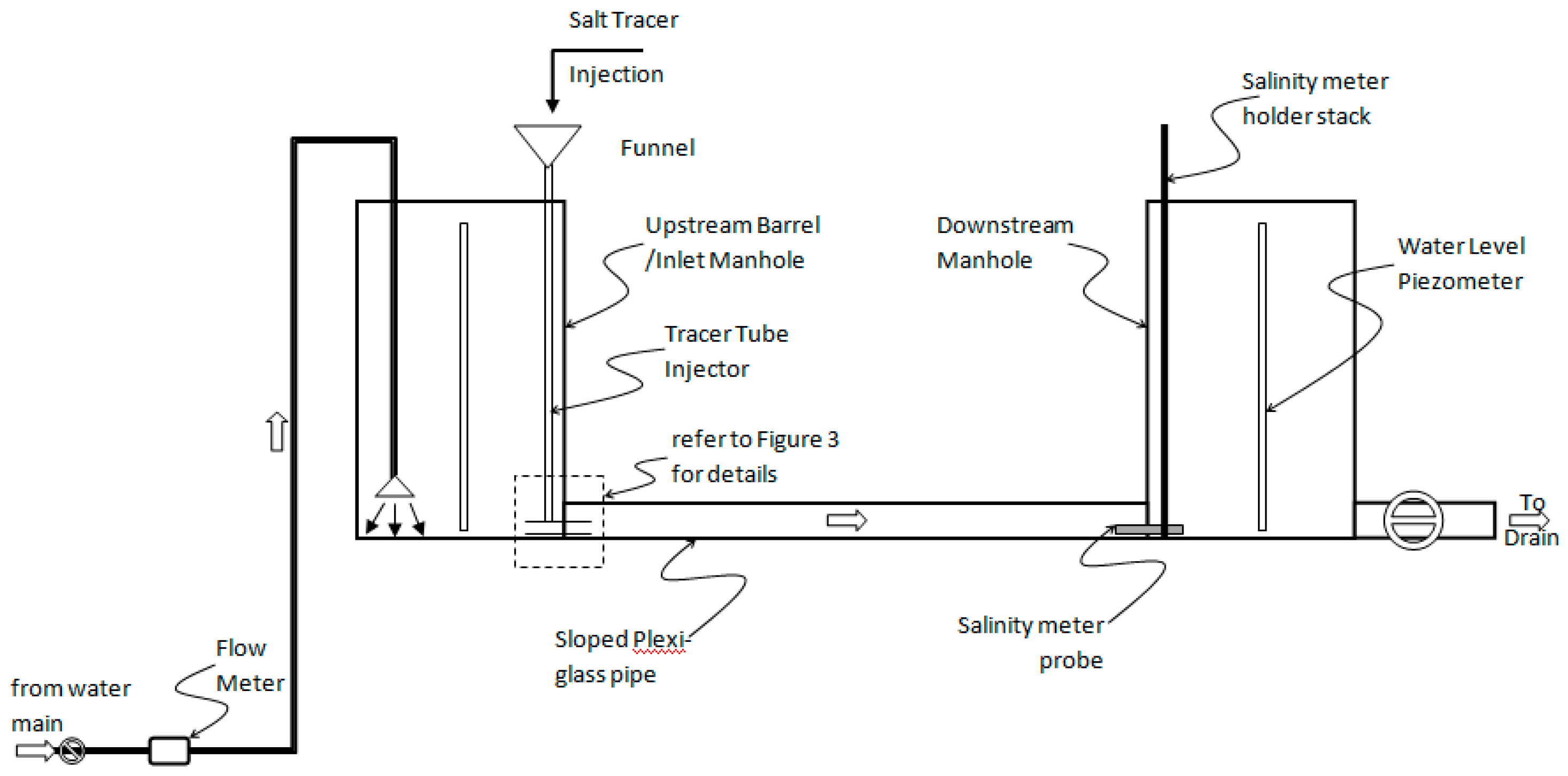
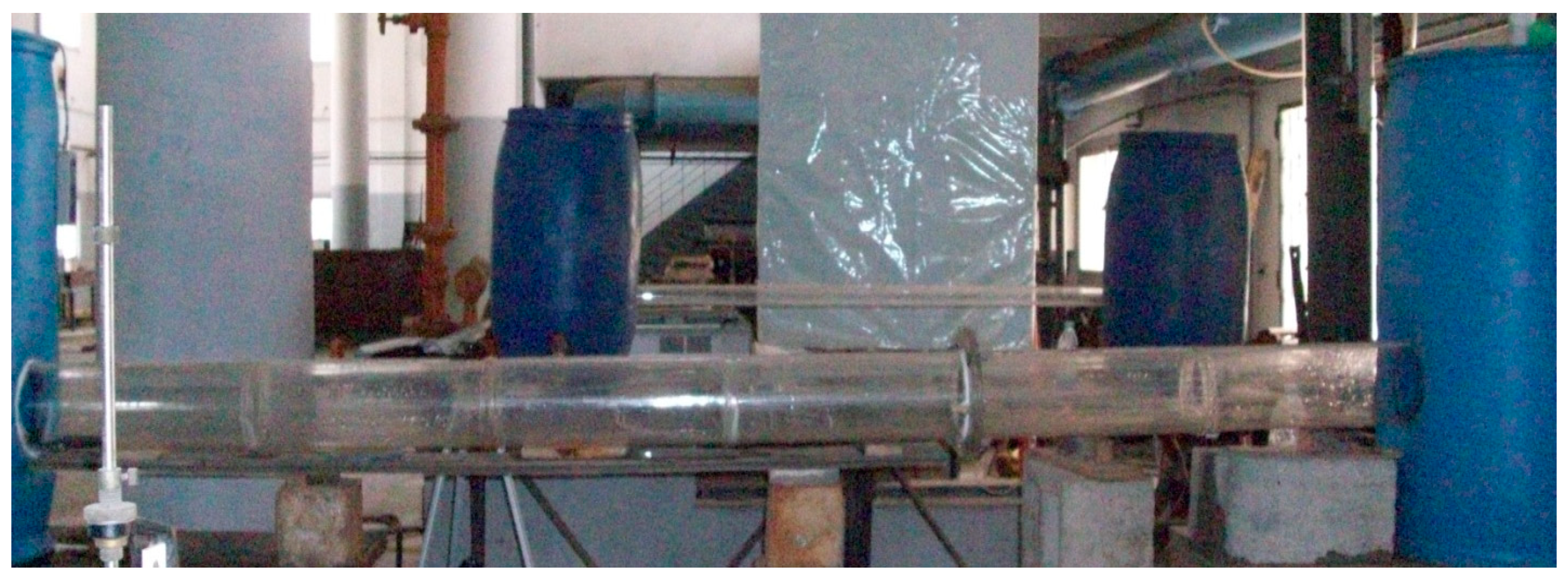
2.1. Experimental Setup

The experimental setup was constructed in the Irrigation and Hydraulics Laboratory of Cairo University. Two experimental sets of runs were created using Plexiglas tubes. Figure 1 shows the typical schematic presentation of the experiment setup. The first experimental set is created for a 60 mm diameter plexiglass pipe of 1.5 m length and is laid at a 3% slope, whereas the second set of runs is created for a 150 mm Plexiglas pipe of 3 m length and is laid at a 1.5% slope. Two 200-litre PVC barrels were used as upstream and downstream manholes (Figure 1 and Figure 2). Sodium chloride (NaCl) was used as a tracer because it is inexpensive, easily available, and does not endanger human health. Salt solutions with tracer concentrations ranging from 1580 ppm and 16,800 ppm were prepared and injected using a salinity injector stick (Figure 1).

Water was supplied from the municipal potable mains and controlled by a valve. The outlet flow (from the downstream barrel) was directly drained to final disposal without circulation to avoid the accumulated build up of the (background) concentration of the tracer. The discharge through the pipe was measured using a calibrated flow meter located upstream. The axial fluid velocity was expected to be repressed from the centerline, but it was slightly increased adjacent to the pipe wall [29].

2.2. Tools and Equipment

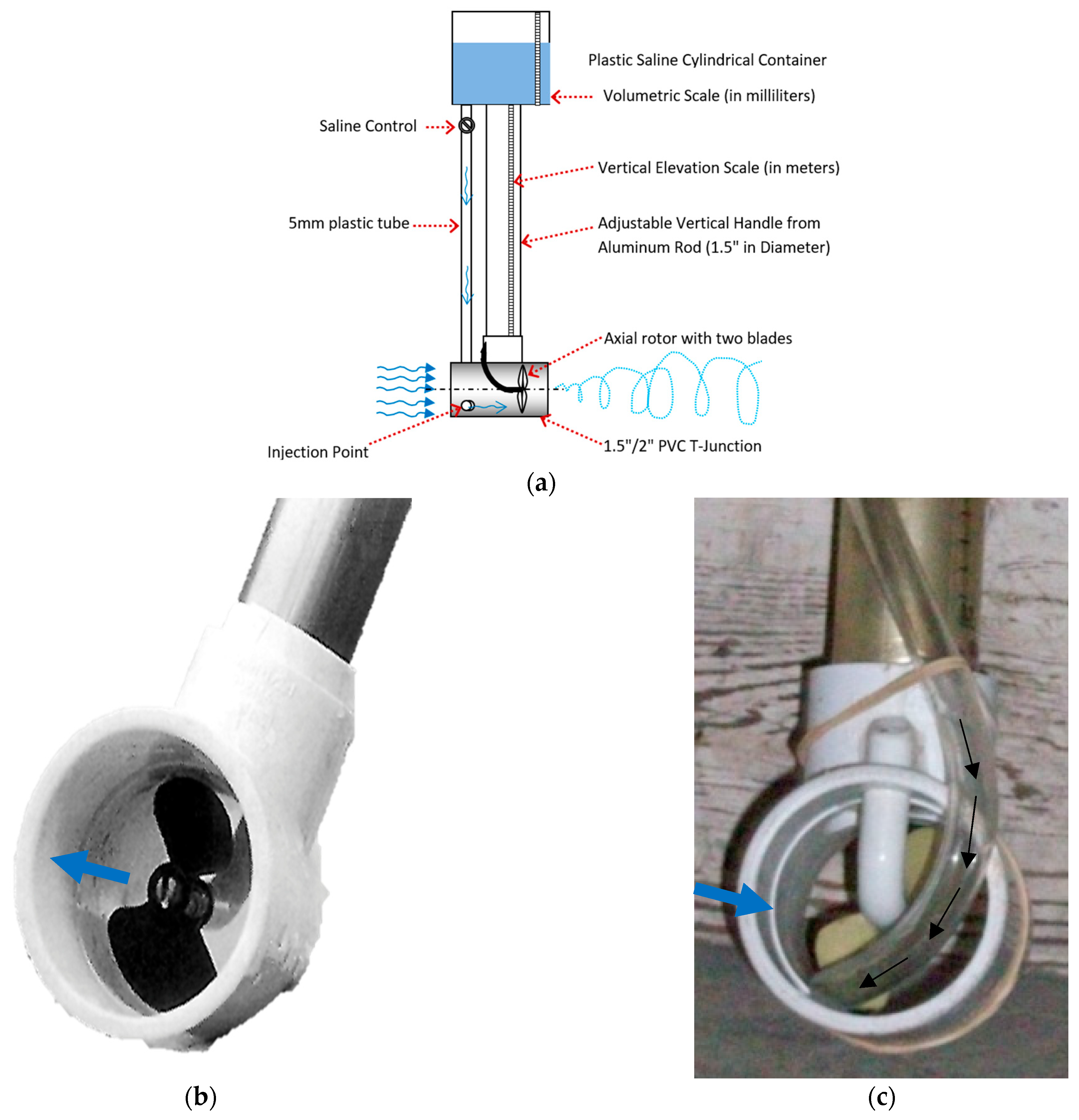
2.2.1. Salinity Injector Stick

The saline injector stick was assembled to help in injecting the saline tracer at the required injection point. The stack consisted of a plastic cone or saline container that was attached to a vertical 5 mm PVC tube that laterally discharged into the upstream face of a 2-inch horizontal PVC tee junction. During measurements, the tee junction was usually aligned in stream with the main flow (Figure 3a).

2.2.2. Passive Fan

The main objective of this study was to investigate the effect of using a passive fan on flow measurement accuracy by way of the saline pulse technique. In order to ensure fast mixing of the salt tracer with the incoming water flow, a passive fan could be added and encased inside the tee junction of the saline injector stick (Figure 3a–c). The fan had an axial flow rotor that consisted of two blades, and the fan unit was encased inside the saline injector tee junction just downstream of the drainage point of the vertical 5 mm saline injector tube (Figure 3). The fan is described as a passive fan because it does not require power to rotate its blades. The blades often rotate freely when exposed to the flowing water stream. It was expected that the rotation of the blades could enhance mixing and thus reduce the required minimum mixing length.

2.2.3. Salinity Meter

A portable microprocessor-based instrument for measuring the TDS (AD 410) salinity meter was used to measure the temporal variation of salinity concentration. The probe had an accuracy of ±1% with a sampling frequency rate of one reading every 0.15 s. The meter was used to measure the initial concentration of the tracer (before injection) and to measure the temporal variation of the downstream tracer concentration at the downstream side of the pipe.

2.3. Assumptions and Simplifications

This experimental study considered the following main assumptions:

• Water flow in the sewer pipe is steady and free from debris and sludges;
• Tracers are conserved, stable, and do not react with other substances in the environment;
• The injection rate of tracer (q) was constant and very small compared to water sewer flow, this means that q/Q << 1.

2.4. Experimental Runs

Two sets of runs with a total number of 85 lab experiment runs were carried out to compare the measured discharge (using flow meter) with the indirect discharge measurement (using the tracer pulse method) (

Table 1. General characteristics of the conducted experiments in the lab.

Set of Run #	Runs Group #	Sewer Pipe Size (mm)	Concentration of Injected Tracer (ppm)							Location of				Injection Stack
			2030	4280	5630	6800	7200	9730	16,800	Saline Injection		Concentration Measurement
										Inside the u/s Manhole	Inside the Pipe Inlet	Inside the d/s Manhole	Inside the Pipe Outlet	Adding a Passive Rotor
1	1	60	√	√	√	√				√		√
	2		√	√	√	√					√	√
	3		√	√	√	√					√	√		√
	4		√	√	√	√				√			√
	5		√	√	√	√					√		√
	6		√	√	√	√					√		√	√
2	7	150	√				√	√	√		√		√	√
	8		√				√	√	√		√		√
	9		√				√	√	√	√		√

). While keeping the pipe slope unchanged, the discharge was varied from 0.13 L/s to 2.2 L/s for the small pipe size case (60 mm) and from 1.4 L/s to 9.1 L/s for the larger pipe size case (150 mm) to examine the different water flow conditions in the pipe. It should be mentioned that the partially full and totally full pipe cases were both examined in the current study and all the experimental measurements were conducted after reaching steady state flow conditions. The location of the injection point and the location of the salinity measurement were both changed to study their effect on the accuracy of flow measurement. Moreover, the effect of utilizing a passive in-stream fan was also examined (refer to Table 1). The selected pipe diameters were selected to generate flow turbulence according to the designed discharge. The concentration of tracer less than 2030 ppm showed an insignificant influence in the case of high discharges, however concentrations higher than 16,800 ppm generated a uniform flow for small flow rates.

2.5. Governing Equations

Water flow discharge Q (L per s) could be indirectly calculated from the tracer test using the mass conservation Equation (2) [23].

$$Q=\frac{M}{A}$$

(2)

where M is the injected mass of salt (in mm) and A is the area under the concentration graph (in mm-s/L).

Figure 4 shows a typical example of the concentration graph representing the temporal variation of downstream salinity measurements.

The quantity A can be calculated as:

$$A={\displaystyle \int }\left(C_2-C_o\right)·dt={\displaystyle \sum }\left(C_2-C_o\right)∆t$$

(3)

where C_o is the background concentration of water in sewer before tracer injection, C₂ is the cross-sectional average concentration of water (at downstream) after tracer injection at time t, and ∆t is the time interval between successive data points.

In the Section to follow, the results of the experimental runs are discussed, and the findings are highlighted.

3. Results and Analysis

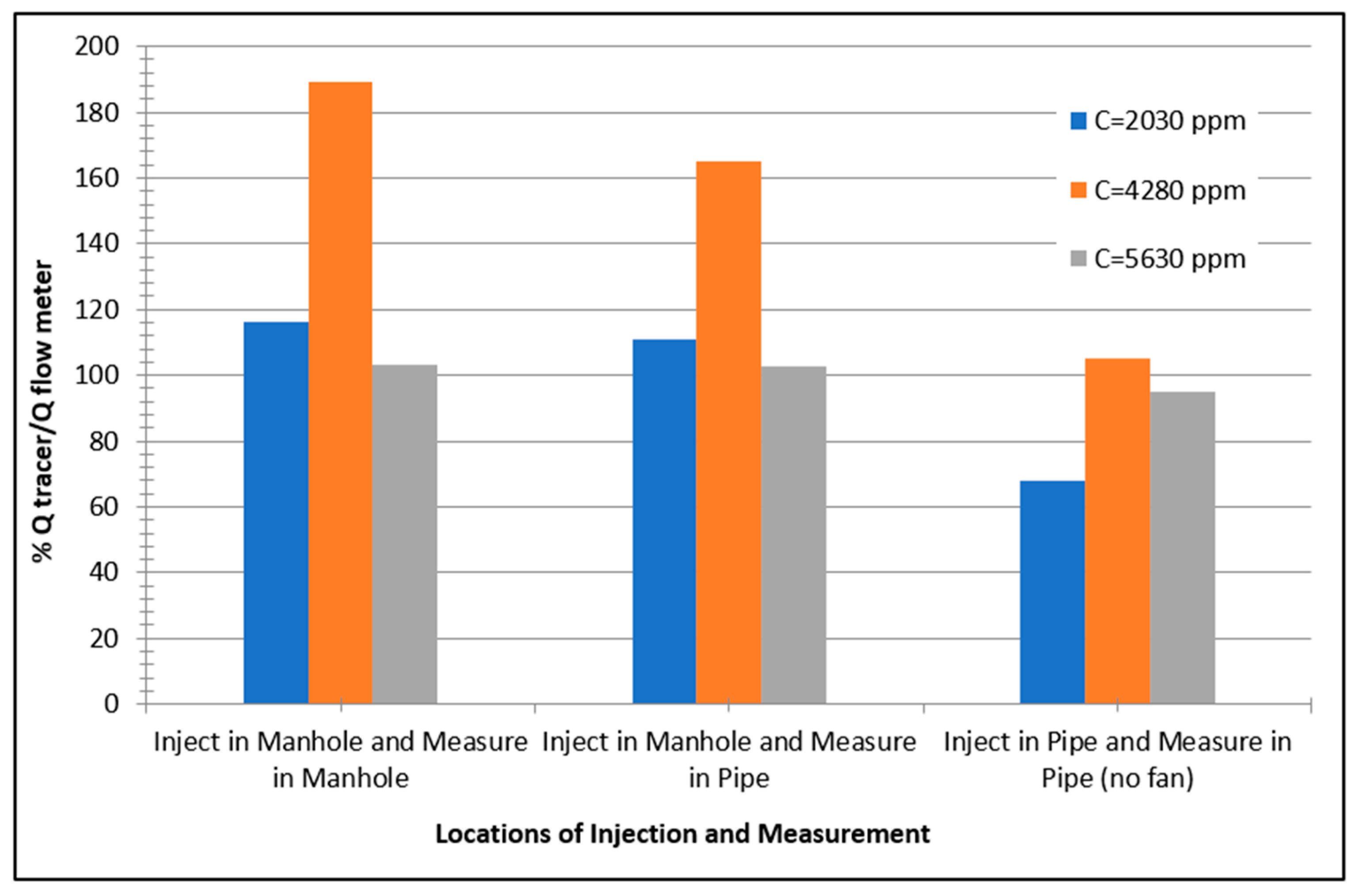
3.1. Effect of Locations of Injection and Measurement Points

It is important to investigate the effect of the locations of injection and measurement points on the flow accuracy. Figure 5 compares the estimated flow results based on the pulse salinity approach (as percentages of the flow meter measurements) for the following three cases:

–

Case 1: The saline injection point is inside the upstream manhole and the measuring concentration point is conducted inside the downstream manhole;

–

Case 2: The saline injection point is inside the upstream manhole and the measuring concentration point is conducted at the downstream end of the pipe;

–

Case 3: The saline injection point is at the upstream end of the pipe and the measuring concentration point is at the downstream end of the pipe.

Based on the experimental results shown in Figure 5, it is noted that the setup arrangement described in Case 3 generally produced more favorable results than the setups of Cases 1 and 2. It is important to mention that injection of saline inside the upstream manhole (as per the setups in Cases 1 and 2) generally resulted in less accurate flow measurements.

The low accuracy in flow measurements obtained in Cases 1 and 2 might be due to the fact that the injection of saline in the upstream manhole resulted in a significant dilution of saline concentration in the upstream manhole before saline entered the sewer pipe. It should also be mentioned that not all water in manholes contributes to the downstream flux due to the possibility of the formation of dead flow zones. Accordingly, the salinity probe located downstream (in Cases 1 and 2) are subjected to a time series of smaller ordinates of salinity concentrations compared to the conditions in Case 3. Needless to say, as concentrations get smaller, errors in measuring them get bigger.

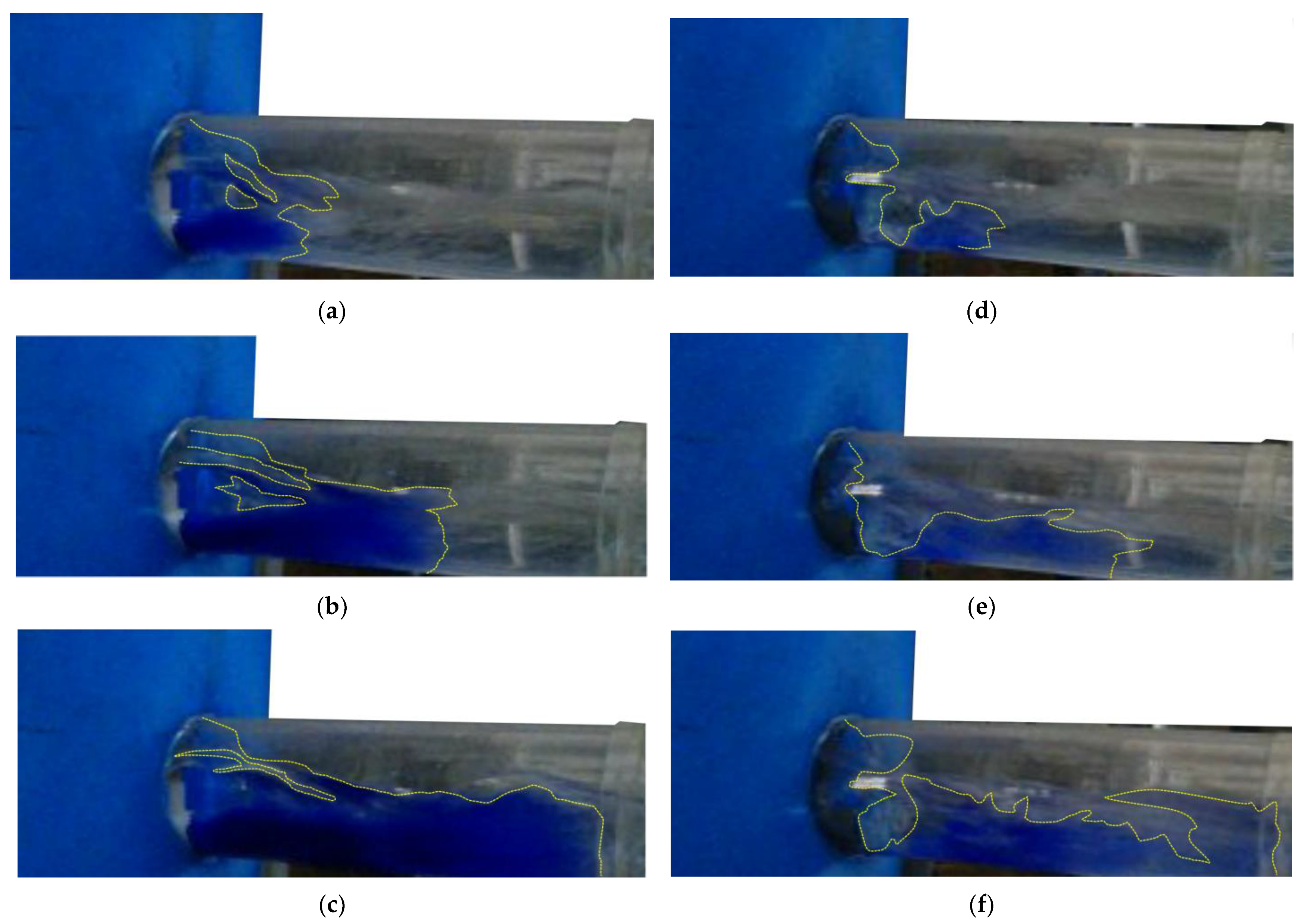
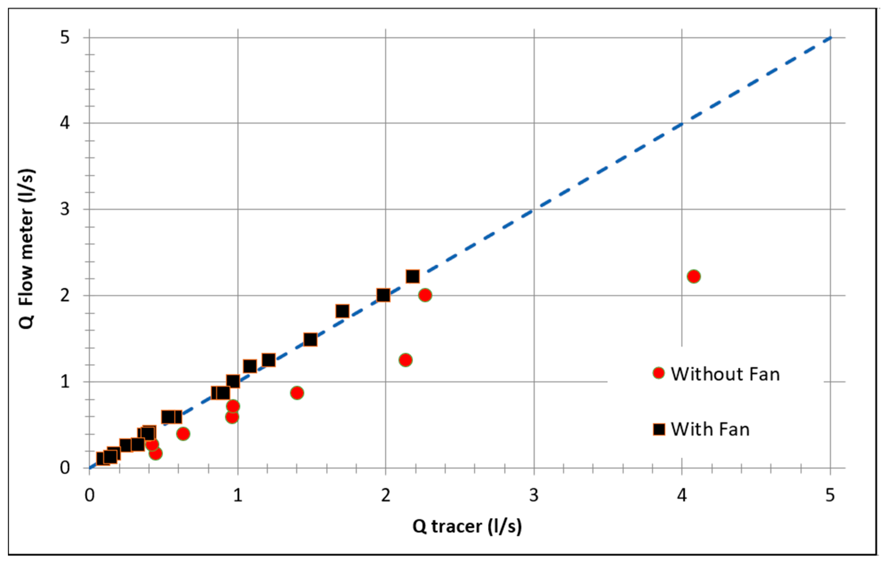
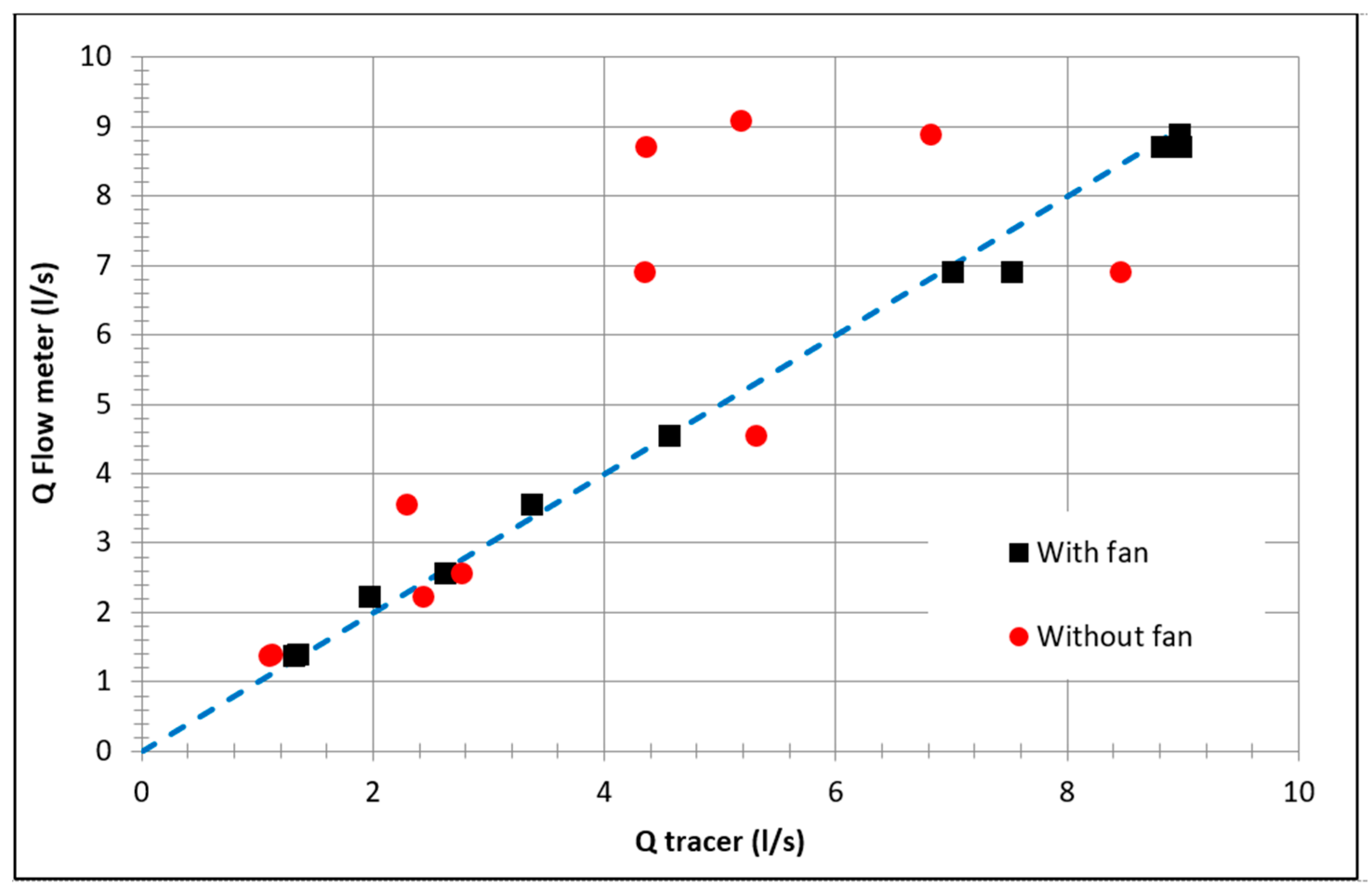
3.2. Effect of Using Passive Fan Module

According to Item 4.1, it is recommended that the saline pulse be injected at the upstream end of the pipe. This can be achieved by using the salinity injector stick (described in Item 2 and Figure 1 and Figure 2). It is also suggested that the concentration of salinity in excess be measured at the downstream end of the pipe rather than inside the downstream manhole. This can be achieved by inserting the salinity probe about 5 cm upstream of the downstream pipe end (as shown in Figure 1).

A visual investigation was conducted to visualize the effect of using the passive fan to enhance mixing. To this end, a blue dye (in the form of NH₃ + SO₄) was injected to visualize the mixing downstream of the saline injector stick. Figure 6 compares the mixing of the solution downstream of the injector sticks in the case of using the fan vs. not using the fan. It is interesting to note that using the passive fan helped in obtaining more uniform mixing across the sewer pipe depth.

Figure 7 and Figure 8 show the comparison of the flow in the case of using the tracer technique and the flow meter technique for pipe sizes 60 mm and 150 mm, respectively. The diagonal line runs from the bottom left to the top right of the plot. It has a slope of unity that represents the “line of equality,” where all points that lie on it means the estimated flow from the indirect tracer method was the same as the measured flow from the flow meter method. Figure 7 and Figure 8 generally show that utilizing a passive rotor (fan) during the injection of the tracer significantly enhances the predictions of the tracer technique. Such an enhancement could be justified as the passive rotor helps in enhancing mixing by creating a spiral motion that extends to a relatively long distance. This spiral motion is expected to better mix the tracer with the incoming water flux. Moreover, the rotor is expected also to increase the water turbulence, which also enhances mixing. A recent CFD study on the passive rotor [5] has concluded that the spiral motion generated by the passive rotor could extend to a relatively long distance (about ten times the diameter of the injection stack outlet). The passive rotor also helps in significantly increasing the turbulence intensity in a distance of about four times the diameter of the pipe stack outlet in the near field zone downstream.

It is interesting to note that the tracer technique seemed to generally overestimate the flow rate for the small pipe case (60 mm) and underestimate it for the bigger pipe case (150 mm), especially in cases where the passive rotor fan was not sured. Such an observation could be explained as follows: the tracer with the lower concentration of salt (case of Figure 7) mixes more easily with the water in the pipe than the tracer with the higher concentration of salt (case of Figure 8).

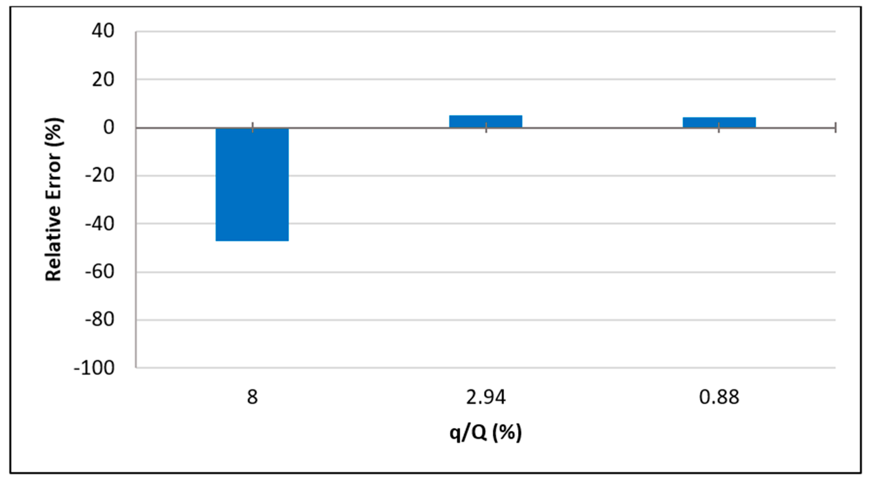
3.3. Effect of Injection Rate

It is important to identify the most recommended injection rate of tracer (q) to be adopted in the flow measurement process. To study the injection-rate effect of the tracer on the accuracy of the indirect estimation of the water flow, the normalized relative error (R_err) was applied. The normalized relative error is a dimensionless variable that could be defined mathematically as R_err = (Q_tracer − Q_flow meter)/Q_flow meter). It is clear to say that the smaller the relative error, the higher the accuracy will be, and that a positive value of R_err implies an overestimation by the tracer technique compared to the flow meter value, whereas vice versa would mean an underestimation of the same.

Figure 9 shows the variation of R_err as a function of the tracer flux to sewer flow ratio (q/Q). According to the Figure, as the ratio q/Q decreases, the relative error decreases and accuracy increases. The significant decrease of accuracy in the case of using a high value of the ratio q/Q might be justified as follows: for a given Q, as the ratio q/Q increases, the injection rate of tracer increases, which means the injected tracer achieves a high velocity that allows it to travel the distance from the injection point to the measurement point in a shorter time and with possibility of limited vertical mixing.

It is noted that the recommended value of q/Q is quite close to 1% and should not exceed 3%. Increasing the injected tracer rate ratio above 3% requires a longer mixing length to achieve a good mixing of the tracer with the water flow.

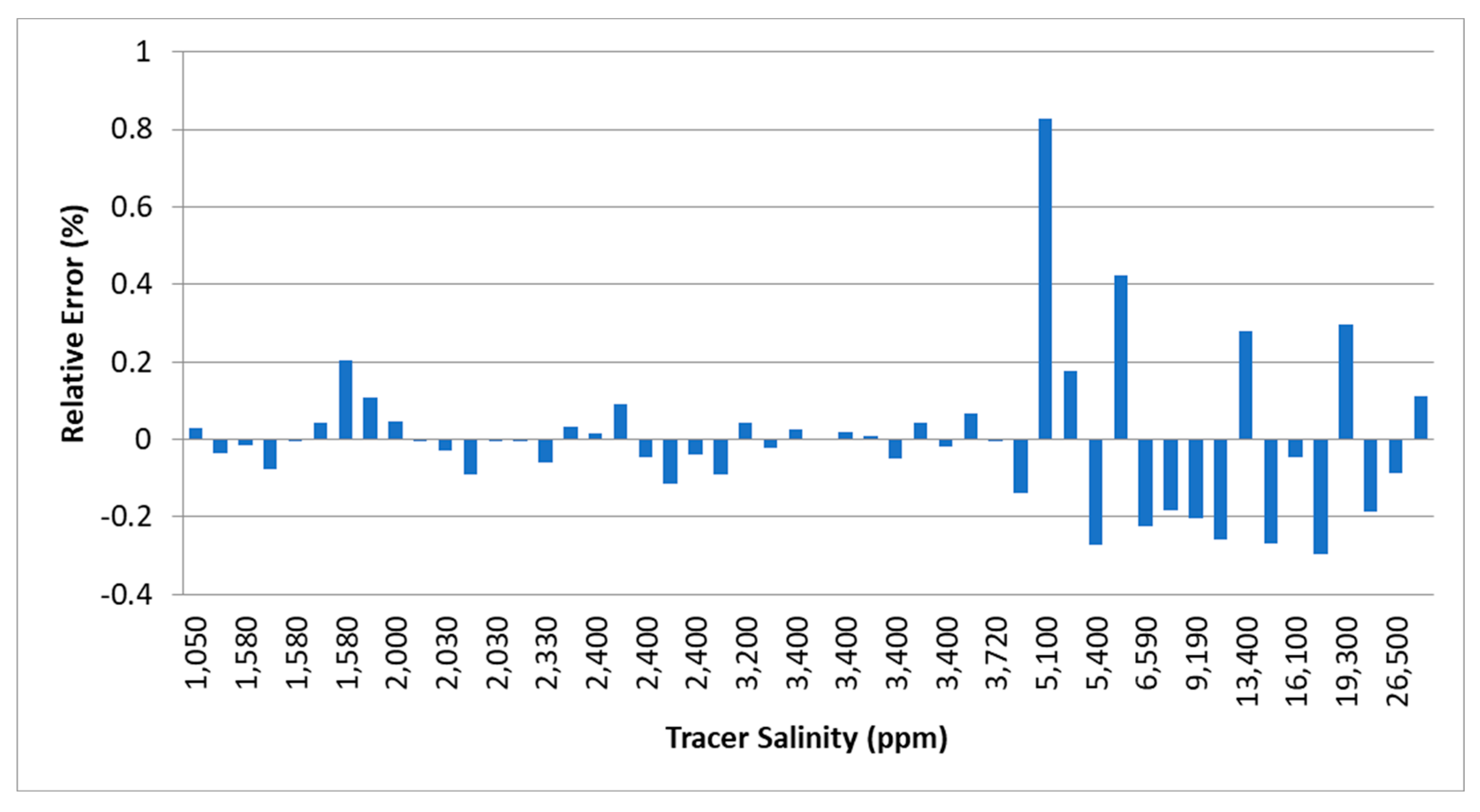
3.4. Effect of Tracer Concentration

Based on common practice, the concentration of the tracer should be high enough to be easily detected and measured, but low enough to not have a significant impact on the properties of the water being measured. Figure 10 shows the effect of the concentration of the injected tracer on relative error for both the 60 mm and 150 mm pipe cases. The Figure shows that relative error significantly increases above a concentration of 4000 ppm. The common practice for using a tracer dilution method for discharge measurements in river is to use a concentration of 3000 ppm [30], which does not contradict the presented result. Based on the study in hand, it is recommended to use an initial tracer concentration that ranges from 1000 ppm to about 3500 ppm to achieve high precision. The noted significant reduction in accuracy in the case of using concentrations of tracers greater than 4000 ppm could be due to the need for longer mixing lengths to completely mix denser solutions.

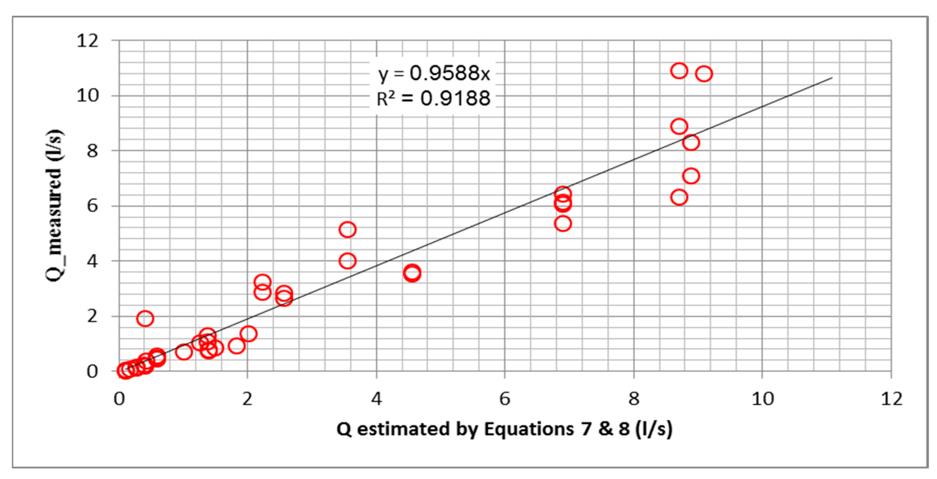
3.5. Tracer-Based Flow Formula

The tracer-based flow formula are regression formulas that are derived to indirectly estimate the gravity sewer pipe flow from the pulse of tracer measurements. For practicality and ease, the targeted formula should not require the full-time series of the pulse of tracer concentration measurements; rather, they should use the peak concentration value (C_2max) and the pulse duration time (T).

Two formulas were derived. The first is based on a dimensional analysis concept whereas the second is based on a semi-empirical perception. The two approaches are discussed in the following Sections.

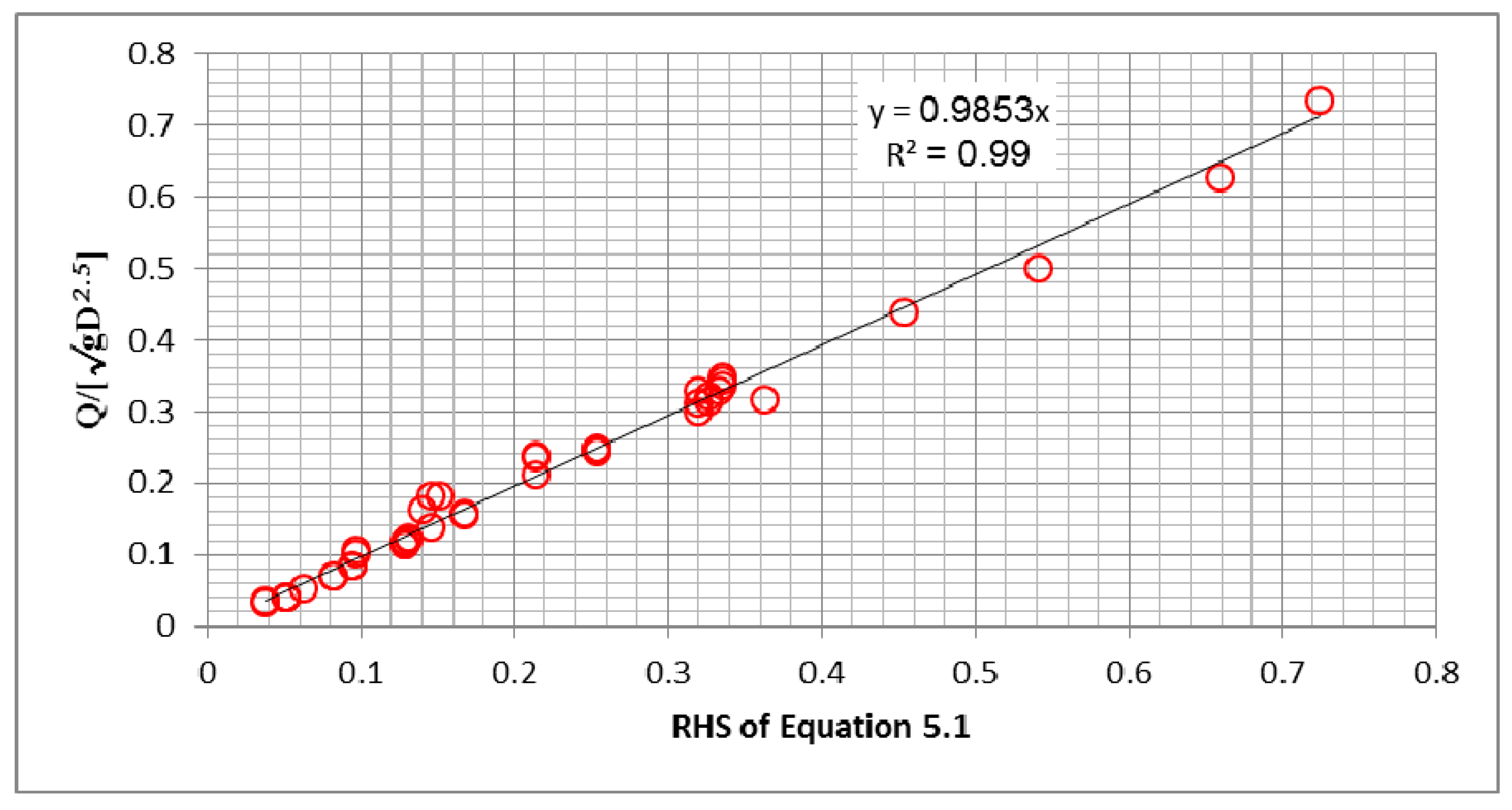
3.5.1. Regression Flow Formulas based on Dimensional Analysis

In this Section, the dimensional analysis concept is presented to develop a regression tracer flow formula that ties the estimated flow with the other key parameters.

By following a dimensional analysis approach, it could be claimed that the sewer dimensionless flow is a function of the following 5 main π-terms:

$$\frac{Q}{\sqrt{g}{D}^{2.5}}=\mathrm{f}(\frac{C_{2max}-C_o}{C_t}, \frac{\sqrt{g}T}{\sqrt{D}}, \frac{L}{D}, \frac{y}{D}, R_n)$$

(4)

where Q is the estimated water flow in sewer pipe based on the pulse of tracer method (m³/s); g is the acceleration of gravity in (m/s²); T is the base time duration of salinity pulse (in sec) (refer to Figure 4); D is the pipe diameter in (m); C_2max, C_o, and C_t are the maximum downstream, background, and injected saline concentrations, respectively, in (ppm or mg/L); R_n is the flow Reynolds no.; and y is the water flow depth at the pipe outlet.

It is worth mentioning that the second term on the right-hand side of Equation (4) represents Froude No., which is based on a velocity scale equals (gT). It is also interesting to note that the appearance of the pipe length in the L/D term could act as a scale for the mixing length of the injected tracer.

After using a least square regression analysis, the relationship demonstrated in Equation (4) can be cast in one of the following formula:

$$\frac{Q}{\sqrt{g}{D}^{2.5}}=\mathrm{a}·R_n^b·{\left(\frac{C_{2max}-C_o}{C_t}\right)}^c·{\left(\frac{L}{D}\right)}^d·{\left(\frac{y}{D}\right)}^e·{\left(\frac{\sqrt{g}T}{\sqrt{D}}\right)}^f$$

(5)

Two regression formulas (based on Equation (5), refer to

Table 2. Coefficients of flow regression formulae based on dimensional analysis.

	Coefficients						R2
	A	b	c	D	e	f
Regression formula #1	0.000139	1.082695	−0.119478	−3.541295	0.500887	0.019549	0.99
Regression formula #2	0.893182	0	−0.452712	0	1.403768	−0.366871	0.86

) were derived based on the pulse of tracer technique. The corresponding coefficients for each formula are given in Table 2. The corresponding coefficient of determination (R² values) is also listed in the last column of the same table. The application of the first regression formula is presented in Figure 11, which shows the agreement of the formula with the measurements.

It should be noted that the first regression formula is nonlinear in the sense that it is a function of Reynolds No (R_n), which in its turn is a function of the flow. In order to break this nonlinearity, it is recommended to initially use the second regression formula (which is not a function of R_n) to obtain an initial guess of the flow, then to use the first regression formula in the second step to obtain a better guess for the flow.

3.5.2. Semi-Empirical Approach

In this Section, the semi-empirical approach is presented to obtain a tracer-based flow formula. The semi-empirical analysis is conducted in two stages:

The first stage is the analytical stage, where the tracer mass-conservation equation is used to determine the downstream flow rate based on the following assumptions:

(1)

The ratio of the injected tracer flux (q) to the water stream flow rate (Q) is quite small, to the extent that q/Q is negligible (i.e., q/Q << 1);

(2)

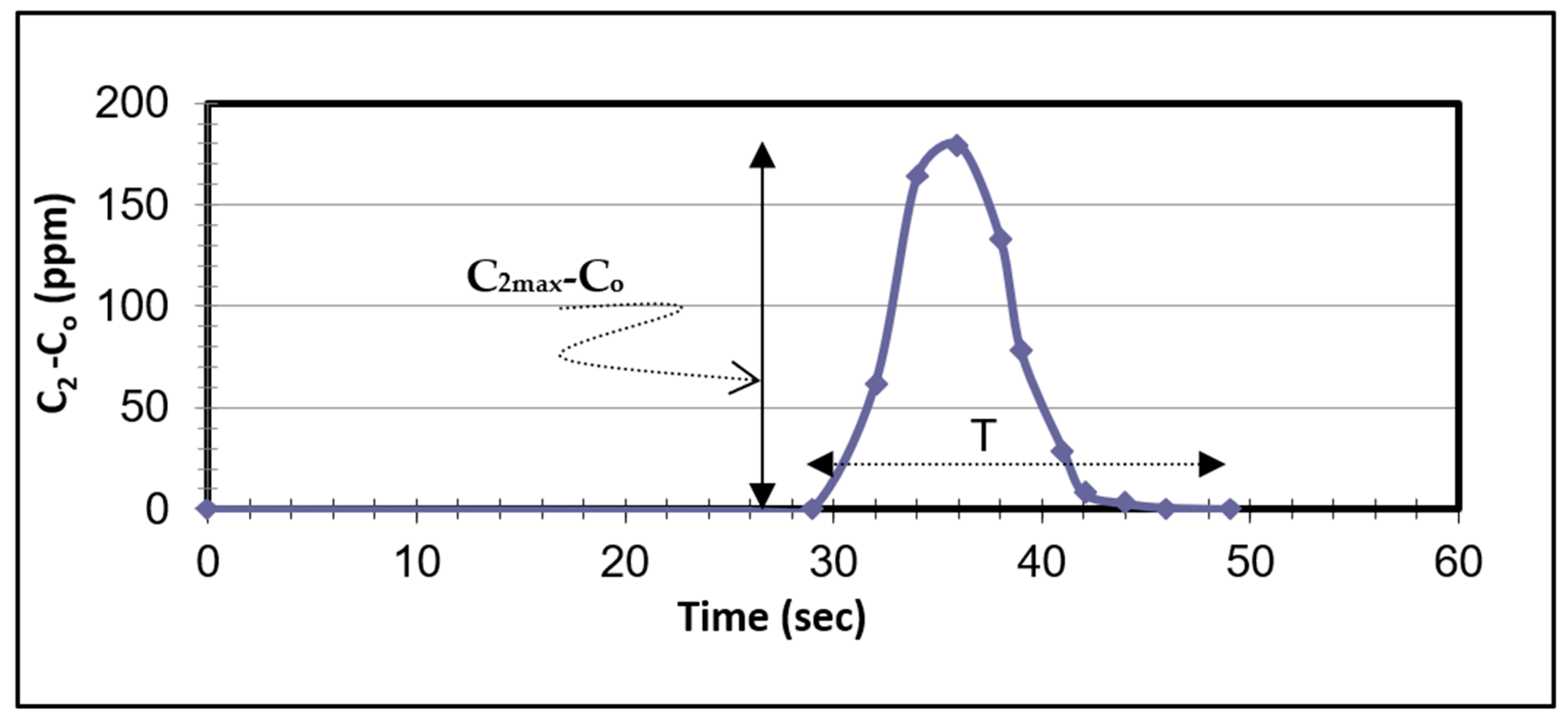
The salinity profile (in excess of the initial background concentration) is idealized and assumed to be triangular. Although this assumption is crude, it is used for the sake of simplicity and the correction factor will be next introduced for this regard;

(3)

The area under the actual measured salinity profile is equal to the area under the idealized triangular salinity profile multiplied by a correction factor F.

Based on the above-mentioned assumptions, the mass-based flow formula reads:

$$Q=q\frac{\frac{t_o}{T}}{(\frac{1}{2})(\frac{C_{2max}-C_{\mathrm{o}}}{C_t})}$$

(6)

where Q is the stream discharge (m³/s), q is tracer injection rate (m³/s), C_t is the concentration of the injected tracer (ppm or mg/L), C_2max is the final peak concentration of tracer pulse at downstream section (ppm or mg/L), C_o is the background tracer concentration at the upstream section (ppm or mg/L), t_o is the time of tracer injection (s), and T is the base time duration of salinity pulse (s).

As a second step, a coefficient (F) is added to Equation (6) to release the triangular-in shape pulse assumption and thus Equation (7) is obtained:

$$Q=q\frac{\frac{t_o}{T}}{(\frac{F}{2})(\frac{C_{2max}-C_{\mathrm{o}}}{C_t})}$$

(7)

The correction factor F could be simply defined as a dimensionless number that represents the ratio between the area under the actual measured salinity profile (by the salinity probe) and the corresponding area under the idealized triangular profile assumption that has the same T and ($C_{2max}$ − $C_o$) values. In addition, the coefficient F is also affected by the degree of mixing at the location of the measurement of the salinity probe.

The values of F are calculated in such a way that the flow rate calculated by the semi-empirical relation exactly matches the flow rate from the flow meter measurements.

The second stage in the semi-empirical approach is the empirical stage, where the dimensional analysis technique is first used to suggest for the main π–στηε εμπıρ should be included and considered in the correction factor (F) formula. By the end of this step, a power-low formula (with unknown coefficients and powers) for the F formula is formulated as a function of the selected π-terms.

In the second step of stage 2, the F values obtained for the group of experimental runs no. 3, 6, and 7 (where the passive rotor is utilized, refer to Table 1) were used to determine the unknown coefficients in the F-formula. A least square error approach was used to minimize the summation of squared differences between the F values from the proposed F-formula (by dimensional analysis) and the corresponding values of F that were obtained from stage one. In this regard, the Excel solver was used to search for the unknown coefficients of the power-low F-formula and the target function was selected to be the summation of squared difference of the F formula and the corresponding values of F from stage 1. In order to locate the optimal minimum solution, the non-linear gradient solver was used and the non-negativity constraint was not adopted to allow for positive as well as negative power values. Equation (8) presents the outcome of the minimization process by Excel solver.

$$F=0.001512·{\left(\frac{L}{D}\right)}^{3.394865}·{\left(\frac{y}{D}\right)}^{-0.855746}·{\left(\frac{\sqrt{g}T}{\sqrt{D}}\right)}^{-1.065692}$$

(8)

Figure 12 presents the comparison of the estimated sewer flow by the semi-empirical equation (Equations (7) and (8)) with the measured flow by the flow meter. The semi-empirical equation reasonably produced the actual measured values.

The following Section summarizes the study’s main findings. Additionally, it describes the limitations of the study and suggests a number of additional research directions for future work.

4. Conclusions, Challenges, and Future Work

An experimental lab investigation was conducted to study the suitability of the tracer slug dilution method in measuring water flow rate in full and partially full sewer pipes and to examine the effect of using (during tracer injection) a passive fan to enhance the accuracy of indirect flow measurement. Based on the conducted study, the following was concluded:

–

The injected tracer rate ratio (q/Q) should be selected such that it does not exceed 3%. The recommended value is around 1%;

–

The recommended concentration of the injected tracer ranges from 1500 to 4500 ppm;

–

Two locations for tracer injection were examined. It has been noted that the most highly recommended injection point is at the upstream end of the pipe and the most highly recommended point for concentration measurement is inside the manhole close to the downstream end of the pipe and not at the manhole’s center;

–

A saline injector stack was developed to help inject saline at the selected injection point;

–

A passive axial flow fan was also proposed and could be encased in the injector stack to enhance mixing and to decrease the required minimum mixing length. It is noted that using the passive fan significantly enhanced the pulse of tracer method’s accuracy.

Two tracer-based flow formulas were derived. The first was based on a pure dimensional analysis approach, and the second was a semi-empirical formula based on the mass conservation approach.

It is noted that the developed formulas are compared favorably with the flow meter method and can be used for both partially full and full pipe flow cases.

Overall, this experiment successfully showed that using a passive rotor increases the accuracy of discharge measurements in sewer pipes based on a saline slug tracer technique. However, continued monitoring is required to test this technique under different flow conditions.

It should be also mentioned that using the passive rotors to enhance mixing during the tracer injection might be challenging in practice. One of the common expected challenges is the sediment and sludge that might be transported with the effluent water, which could break or even remove the rotor from its place. One way to overcome such a challenge is to install a protective cover or shield over the rotor to prevent debris from coming into direct contact with the rotor. The effect of using this protective cover need to be assessed and studied in the future.

The results of the study in hand were derived from two pipe sizes (60 mm and 150 mm). Nevertheless, the dynamic similarity concept (more specifically the Froude similarity law for gravity systems) could be used to scale up the findings to bigger pipe sizes. However, it is important to be cautious when extrapolating experimental results beyond the range of pipe sizes that were studied. It is always a good idea to validate such predictions using additional experiments or numerical simulations, if possible. It should be mentioned that as pipe sizes gets bigger and water depth inside the sewer gets deeper, the required minimum mixing length increases. In these cases, a bigger size of passive rotor is recommended to be used to effectively reduce the mixing length. The suitable size of the rotor for bigger pipe sizes could be an interesting point to be studied in the future.

Potential areas of future research include: (a) extending the study to include bigger sewer pipe sizes; (b) studying the effect of using different passive rotor sizes on mixing efficiency; and (c) extending the analysis to cases of river flow or open channels. Another future research topic could be to conduct a CFD study spanning from injection of the tracer to the measuring probe. The objective of such a study could be to analyze numerically the effects of the water-tracer-rotor (fluids-structure) interactions and to develop a better understanding of the tracer dilution method with a passive rotor.

References

1. Sadoff, C.W.; Borgomeo, E.; Uhlenbrook, S. Rethinking water for SDG 6. Nat. Sustain. 2020, 3, 346–347. [Google Scholar] [CrossRef]
2. Ortigara, A.R.C.; Kay, M.; Uhlenbrook, S. A review of the SDG 6 synthesis report 2018 from an education, training, and research perspective. Water 2018, 10, 1353. [Google Scholar] [CrossRef] [Green Version]
3. Rao, A.S.; Marshall, S.; Gubbi, J.; Palaniswami, M.; Sinnott, R.; Pettigrovet, V. Design of low-cost autonomous water quality monitoring system. In Proceedings of the 2013 International Conference on Advances in Computing, Communications and Informatics (ICACCI), Mysore, India, 22–25 August 2013; pp. 14–19. [Google Scholar]
4. Sun, J.Y.; Jepson, W.P. Slug flow characteristics and their effect on corrosion rates in horizontal oil and gas pipelines. In Proceedings of the SPE Annual Technical Conference and Exhibition, Washington, DC, USA, 4 October 1992. [Google Scholar]
5. Farouk, M.; Kriaa, K.; Elgamal, M. CFD simulation of a submersible passive rotor at a pipe outlet UNDER time-varying water Jet Flux. Water 2022, 14, 2822. [Google Scholar] [CrossRef]
6. Elgamal, M.; Kriaa, K.; Farouk, M. Drainage of a water tank with pipe outlet loaded by a passive rotor. Water 2021, 13, 1872. [Google Scholar] [CrossRef]
7. Elgamal, M.; Abdel-Mageed, N.; Helmi, A.; Ghanem, A. Hydraulic performance of sluice gate with unloaded upstream rotor. Water SA 2017, 43, 563–572. [Google Scholar] [CrossRef] [Green Version]
8. Turkyilmazoglu, M. Eyring–Powell fluid flow through a circular pipe and heat transfer: Full solutions. Int. J. Numer. Methods Heat Fluid Flow. 2020, 30, 4765–4774. [Google Scholar]
9. Spencer, E.A.; Tudhope, J.S. A Literature Survey of the Salt-Dilution Method of Flow Measurement; National Engineering Laboratory-NEL: Glasgow, UK, 1954. [Google Scholar]
10. Church, M.; Kellerhals, R. Stream Gauging Techniques for Remote Areas Using Portable Equipment; Department of Energy, Mines and Resources: Ottawa, ON, Canada, 1970; pp. 55–68. [Google Scholar]
11. Church, M. Electrochemical and Fluorometric Tracer Techniques for Streamflow Measurements; Technical Bulletin 12; British Geomorphological Research Group: London, UK, 1975. [Google Scholar]
12. Day, T.J. On the precision of salt dilution gauging. J. Hydrol. 1976, 31, 293–306. [Google Scholar] [CrossRef]
13. Day, T.J. Field procedures and evaluation of a slug dilution gauging method in mountain streams. J. Hydrol. 1977, 16, 113–133. [Google Scholar]
14. Hongve, D. A revised procedure for discharge measurement by means of the salt dilution method. Hydrol. Process. 1987, 1, 267–270. [Google Scholar] [CrossRef]
15. Johnstone, D.E. Some recent developments of constant-rate salt dilution gauging in rivers. J. Hydrol. 1988, 27, 128–153. [Google Scholar]
16. Kite, G. Computerized stream flow measurement using slug injection. Hydrol. Process. 1993, 7, 227–233. [Google Scholar] [CrossRef]
17. Moore, R.D. Introduction to salt dilution gauging for stream flow measurement: Part 1. Streamline Watershed Manag. Bull. 2004, 7, 20–23. [Google Scholar]
18. Moore, R.D. Introduction to salt dilution gauging for stream flow measurement Part II: Constant-rate injection. Streamline Watershed Manag. Bull. 2004, 8, 11–15. [Google Scholar]
19. Moore, R.D. Introduction to salt dilution gauging for streamflow measurement Part III: Slug injection using salt in solution. Streamline Watershed Manag. Bull. 2005, 8, 1–6. [Google Scholar]
20. Lee, S.; KMuthukumar, U.; Chandapillai, J.; Saseendran, S. Flow measurement in hydroelectric stations using tracer dilution method-case studies. In Proceedings of the IGHEM-2010, Roorkee, India, 21–23 October 2010; AHEC, IIT: Roorkee, India, 2010. [Google Scholar]
21. Mastrocicco, M.; Prommer, H.; Pasti, L.; Palpacelli, S.; Colombani, N. Evaluation of saline tracer performance during electrical conductivity groundwater monitoring. J. Contam. Hydrol. 2011, 123, 157–166. [Google Scholar] [CrossRef] [PubMed]
22. Hudson, R.; Fraser, J. Alternative methods of flow rating in small coastal streams. In Hydrology; Extension Note EN-014; Ministry of Forests: Nanaimo, BC, Canada, 2002; 11p. [Google Scholar]
23. Hudson, R.; Fraser, J. Introduction to salt dilution gauging for streamflow measurement part IV: The mass balance (or dry injection) method. Streamline Watershed Manag. Bull. 2005, 9, 6–12. [Google Scholar]
24. Sun, B.; Lu, Y.; Liu, Q.; Fang, H.; Zhang, C.; Zhang, J. Experimental and numerical analyses on mixing uniformity of water and saline in pipe flow. Water 2020, 12, 2281. [Google Scholar] [CrossRef]
25. Scordo, E.B.; Moore, R.D. Transient storage processes in a steep headwater stream. J. Hydrol. Process. 2009, 23, 2671–2685. [Google Scholar] [CrossRef]
26. Fabian, M.W.; Endreny Theodore, A. Seasonal variation in cascade-driven hyporheic exchange, northern Honduras. J. Hydrol. Process. 2011, 25, 1630–1646. [Google Scholar] [CrossRef]
27. MacDonald, R.J.; Boon, S.; Byrne, J.M.; Silins, U. A comparison of surface and subsurface controls on summer temperature in a headwater stream. J. Hydrol. Process. 2014, 28, 2338–2347. [Google Scholar] [CrossRef]
28. Zhang, J.; Kiesha, C.; Pierre, S.; Tejada-Martinez, A.E. Impacts of flow and tracer release unsteadiness on tracer analysis of Water and wastewater treatment facilities. J. Hydraul. Eng. 2019, 145, 04019004. [Google Scholar] [CrossRef]
29. Thatoe Nwe Win, T.; Bogaard, T.; van de Giesen, N. A low-cost water quality monitoring system for the Ayeyarwady River in Myanmar using a participatory approach. Water 2019, 11, 1984. [Google Scholar] [CrossRef]
30. Kilpatrick, F.A.; Cobb, E.D. Measurement of Discharge Using Tracer; US Geological Survey; Department of the Interior: Washington, DC, USA, 1985.
Figure 1. Schematic presentation of the experimental setup.
Water 15 00369 g001
Figure 2. Snapshots of the two Plexiglas tubes.
Water 15 00369 g002
Figure 3. Saline tracer injector: (a) elements of salinity injector stick equipped with a downstream passive rotor. (b) Looking from downstream to upstream through passive rotor. (c) looking from upstream to downstream (tracer injection plastic tube appears).
Water 15 00369 g003
Figure 4. Typical example of measured temporal variation of salinity with time.
Water 15 00369 g004
Figure 5. Comparison of results based on utilizing different injection and measurement points.
Water 15 00369 g005
Figure 6. Comparison of the mixing of blue dye downstream of the injector stick, before and after utilizing the passive rotor (Pipe Size 150 mm, Q = 9.0 L/s). (a) after 6 frames (0.2 s) (with Fan); (b) after 10 frames (0.33 s) (with Fan); (c) after 15 frames (0.5 s) (with Fan); (d) after 6 frames (0.2 s) (without Fan); (e) after 10 frames (0.33 s) (without Fan); (f) after 15 frames (0.5 s) (without Fan).
Water 15 00369 g006
Figure 7. Effect of utilizing passive fan (pipe size 60 mm; tracer saline concentration = 1580 < C < 2030 ppm).
Water 15 00369 g007
Figure 8. Effect of utilizing passive fan (pipe size 150 mm; tracer saline concentration < 3500 ppm).
Water 15 00369 g008
Figure 9. The effect of salinity injection rate on the relative error of flow measurement.
Water 15 00369 g009
Figure 10. Effect of tracer concentration on flow accuracy.
Water 15 00369 g010
Figure 11. Flow Formula based on Dimension Analysis.
Water 15 00369 g011
Figure 12. Semi-empirical formula for estimating flow in sewer pipes.
Water 15 00369 g012