

Quantification of Evapotranspiration by Calculations and Measurements Using a Lysimeter

Institute of Hydrology, Slovak Academy of Sciences, Dúbravská cesta 9, 841 04 Bratislava, Slovakia
*
Author to whom correspondence should be addressed.
Water 2023, 15(2), 373; https://doi.org/10.3390/w15020373
Submission received: 14 December 2022
/
Revised: 4 January 2023
/
Accepted: 12 January 2023
/
Published: 16 January 2023
(This article belongs to the Special Issue Advances in Sustainable Agriculture Progress under Climate Change)
Abstract
:Evapotranspiration is one of the key elements of water balance in nature. It significantly influences the water supply in the unsaturated zone of a soil profile. The unsaturated zone is a water source for the biosphere. The aim of this study is to measure, calculate and analyze the course of actual evapotranspiration, precipitation and dew totals as well as the totals of water flows at the lower boundary of unsaturated zone and the change in water content in specified soil volume. The measurements are used for verifying the results of numerical simulation. The methods used in the study were chosen based on the hypothesis that dynamics of water supply changes in the unsaturated zone is the result of the interactions between atmosphere, soil and plant cover. The elements of water balance were quantified by the methods of water balance, lysimeter measurements and numerical simulation on the model HYDRUS-1D, version 4. The abovementioned parameters were quantified for the East Slovakian Lowland, with an hourly time step during the years 2017, 2018 and 2020. The measurements have shown that evapotranspiration exceeded precipitation during all monitored periods, specifically by 22% in 2017, by 14% in 2019, and by 10% in 2020. The deficit was compensated for by capillary inflow from the groundwater level and the water supply in the unsaturated zone. A verification by measurement has shown that numerical simulation is imprecise in relation to the quantification of water flows at the lower boundary of the unsaturated zone. This inaccuracy is manifested in the higher value of the actual evapotranspiration, which is on average exceeded by 11%. The performance of the mathematical model is assessed as satisfactory for the analysis of the soil water regime.
1. Introduction
The evaporation of water in nature is a thermodynamic process in which water changes from the liquid or solid phase to the gas phase. It is an energy-demanding process that is a decisive regulator of the energy flow in the hydrological cycle [1,2,3]. The evaporation of water is of fundamental importance for the biomass production process [4,5].
The process of evaporation from plants and soil is called evapotranspiration. The maximum amount of water that can evaporate under given meteorological conditions is called potential evapotranspiration (ETp) [6]. For practical reasons, the reference evapotranspiration ET0 is also calculated [7,8,9,10]. The calculation of ET0 is based on the Penman-Monteith equation [11,12,13,14,15,16,17] for a reference surface covered with a hypothetical grass reference crop with an assumed crop height of 0.12 m. Real evaporation from soil and plants is called actual evapotranspiration (ETa). If there is enough water in the soil profile, then ETa = ETp. The inequality ETa < ETp indicates a lack of water in the root zone of the soil profile and the beginning of the drying of the soil profile [18].
Evapotranspiration is one of the key elements of water balance in nature [19,20,21,22]. It significantly affects the water supply in the unsaturated zone of the soil profile [23,24,25]. The unsaturated zone is a water source for the biosphere. It supplies plant cover with water during growing seasons. The water in this source does not have the properties of free water. In order to use it, plants need to have a strong root system and they need to develop a suction pressure which is big enough to disrupt the bond between the water and the soil. Information on evaporation and intensity of evapotranspiration during the growing season is crucial for agricultural production, landscape water management, and the design of adaptation measures [26,27,28,29,30].
To determine the actual evapotranspiration is a demanding process. At present, many methods for its quantification have been studied [31,32,33]. They are based on both measuring and modelling methods. This study is based on the hypothesis that dynamics of water supply changes in the unsaturated zone is the result of the interactions between the atmosphere, the soil, and plant cover. It is a systemic approach to the investigated issue which requires an effective methodology. The method of lysimeter measurements, numerical calculations on the mathematical model HYDRUS-1D and the water balance method were used. These are advanced scientific methods used for the quantification of interaction processes between the atmosphere, soil and plant cover.
The aim of this study is to measure, calculate and analyze the course of actual evapotranspiration, precipitation and dew totals as well as the totals of water flows at the lower boundary of the unsaturated zone and the change in water content in specified soil volume. The measurements are used for verifying the results of a numerical simulation and subsequently to assess the applicability of the model for the quantification of ETa and the elements of the water regime in the conditions of the East Slovakian Lowland.
2. Materials and Methods
2.1. Research Site Characteristics and Study Period
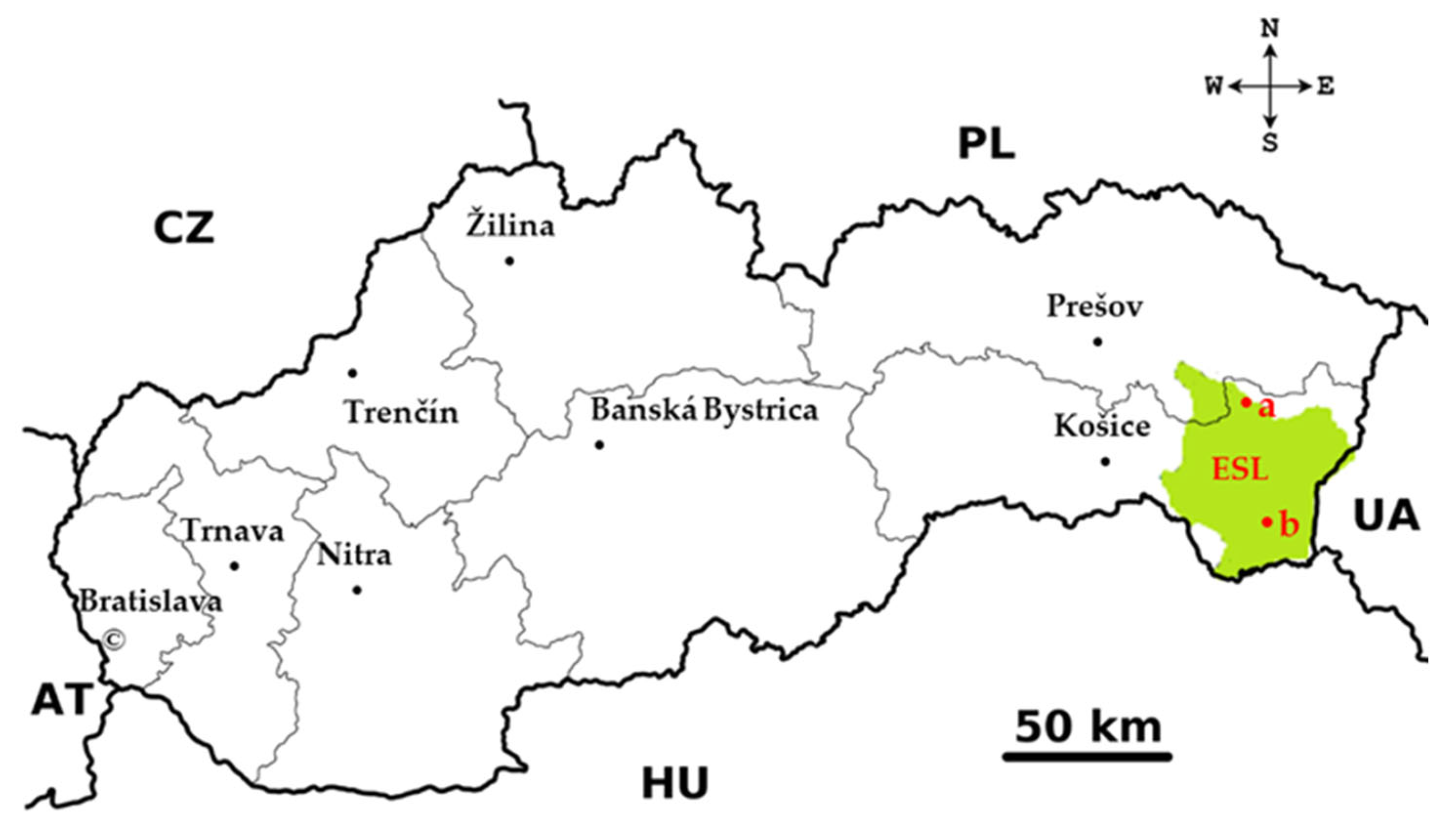
The lysimeter station is located on the East Slovakian Lowland (ESL) in Petrovce nad Laborcom (48°47.540′ N and 21°53.175′ E), at an altitude of 117 m above sea level (Figure 1).
From a geomorphological point of view, the ESL spreads over 2638 km2. The lowland is a part of the Neogene basin, which was created by the uneven tectonic subsidence of the Earth’s crust within the Carpathian arc in the Neogene and Quaternary periods. The subsidence induced the prevalence of accumulation processes and thus the formation of a flat lowland surface comprising river sediments, loess and sands. The altitude varies between 94 and 180 m, the majority of the surface having 100 m to 120 m of altitude. Typical features of the East Slovakian Lowland are depression areas covered with heavy, clay loam soils.
Climate-wise, the ESL is situated in the transitional zone between the oceanic and continental climate. The climate, and thus all meteorological elements, is greatly variable, which is reflected in the rapid change of air masses in every season and general cyclonic activity. A characteristic feature of the area is mainly the degree of continentality. The amplitude of air temperature on ESL, i.e., the difference between the temperature in the warmest and coldest month of the year, reaches 24.0–24.4 °C. As per the Climate Atlas of Slovakia [34], the area is warm and moderately humid with a mild winter. The average number of summer days (Tmax ≥ 25 °C) is 70, and the average annual air temperature is 10 °C. In terms of temperature, ESL is a homogenous area. Major deviations are visible only in the localities close to and influenced by hillsides and mountains surrounding the lowland. The average duration of sunshine is 1916 h. This is 43% of the astronomically possible sunshine, which is 4474 h. The upper boundary of evapotranspiration is characterized by potential evapotranspiration. The annual sum of this parameter is between 619 mm and 687 mm, the maximum being 115 mm to 125 mm in July and the minimum approaching zero in January. The relative air humidity on ESL varies throughout the year as well as throughout the day. During the year, maximum values are reached in December (87% to 88%) and minimum values are reached in April (67% to 71%). The average annual relative air moisture is 77% [34]. For the formation of precipitation, circulation factors play an important role. On ESL, rainfall occurs mainly when the area is hit by humid and warm air currents from the south. Air masses bearing precipitation which come from the west, north and east are depleted of the precipitation that falls on the slopes of the Carpathian mountain range. This is reflected in the spatial distribution of rainfall. The area with the minimum annual sum of precipitation (below 600 mm) is located in the central and southwest parts of the lowland. Towards the west and northeast, the volume of precipitation increases, with annual sums being 800 mm to 900 mm.
This study evaluates three periods: from 27 May 2017 to 21 October 2017 (148 days), from 8 February 2019 to 30 November 2019 (296 days), and from 22 April 2020 to 23 November 2020 (216 days).
2.2. Description of the Lysimetric Station
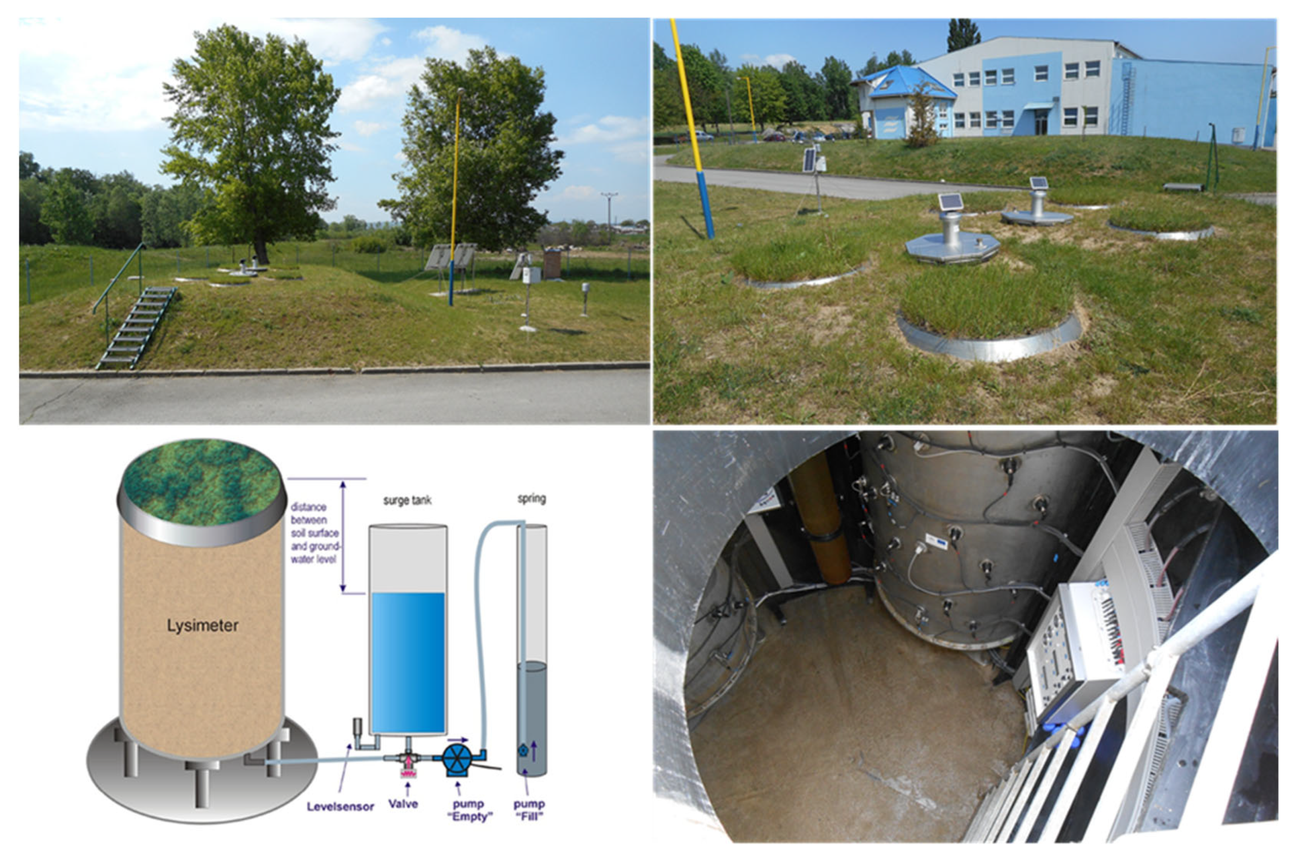
The lysimeter station in the location of Petrovce nad Laborcom (Figure 2) is part of the scientific infrastructure of the Institute of Hydrology of the Slovak Academy of Sciences, Bratislava. The station entered into operation in 2015.
The station consists of five lysimeters stored in two separate plastic containers. Each lysimeter consists of a steel cylinder with a surface area of 1 m2 and a height of 2.5 m [35]. The cylinders contain undisturbed soil monoliths from various locations in the ESL. The samples were chosen to best represent the soil environment on the ESL [36]. The lysimeters are equipped with an adjustable ground water level (GWL) system connected to a nearby well that serves as a water source. All monoliths are placed on three-point scales with a sensitivity of 0.01 kg, which corresponds to a water column of 0.01 mm.
Part of the lysimeter station is a meteorological station providing data on meteorological elements such as air temperature (°C), relative air humidity (%), wind speed (m/s), wind direction (0–360°), global radiation (W/m2), and precipitation (mm).
Data from lysimeter measurements are stored in data loggers. Once a day, data is sent via a wireless connection to the central server. The data is available in an hourly time step. The entire station is powered by batteries charged by solar panels.
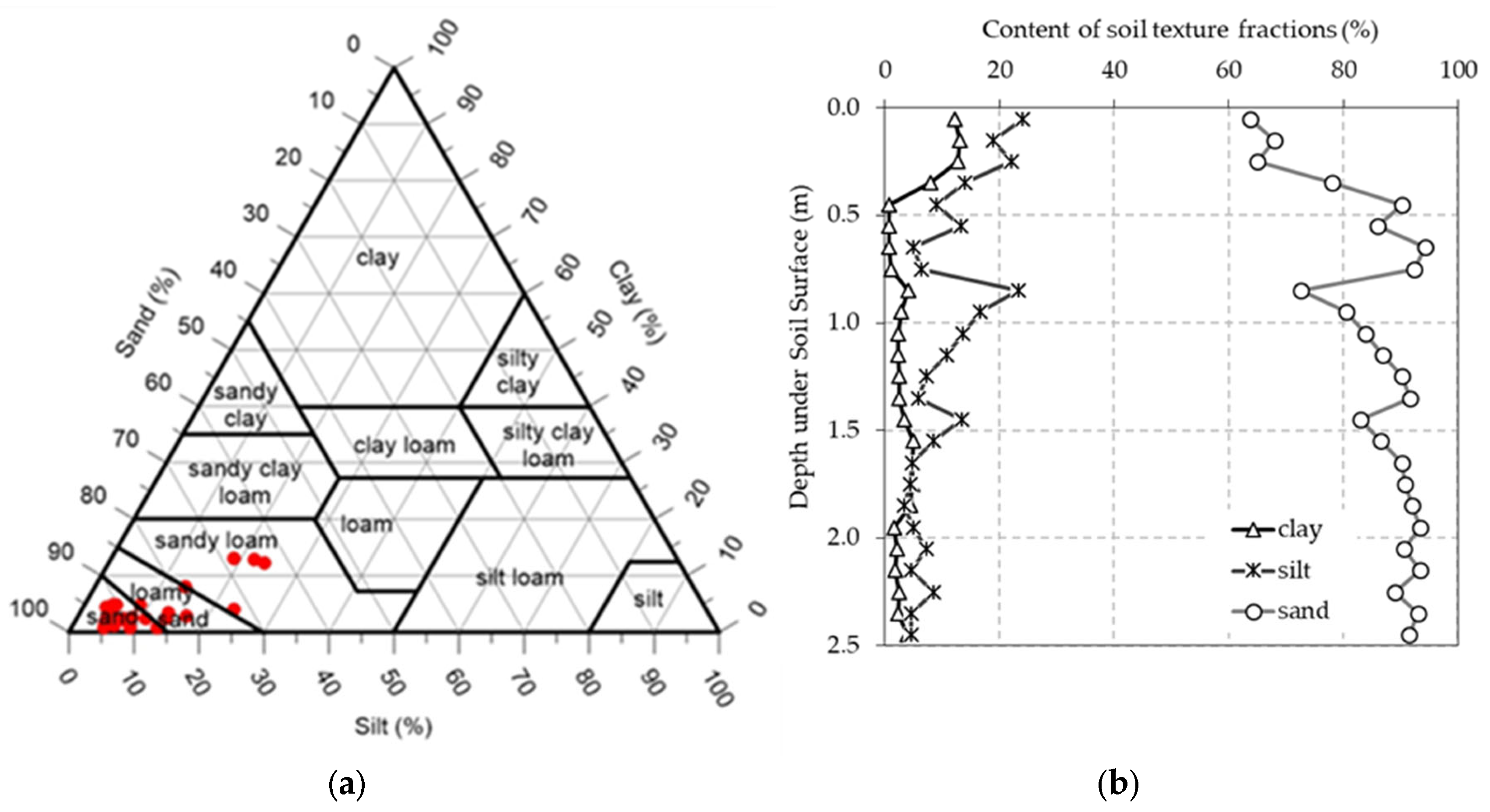
The investigated monolith contains soil taken from a location in the southeast of the ESL (48°28.237′ N and 21°58.326′ E). The soil profile is loamy-sandy to sandy, changing to sandy loam in the upper part (Figure 3). The plant cover on the surface of the soil monoliths consists of grass maintained at the height of 0.12 m.
2.3. Processing of the Lysimetric Data
The lysimeter is a valuable tool for quantifying the components of the soil water regime and their balance in the soil-plant-atmosphere-groundwater system [37,38,39,40,41,42]. Water balance is used to quantify the individual components of water regime in the soil [43]. It expresses the change of water content in the examined volume of soil by the difference between inflow and outflow balance components. The change in the amount of water W in the studied soil volume V depends on the inflow or outflow of water across the upper and lower boundaries of the studied soil zone [44,45,46]. The upper boundary is the area where the soil profile interacts with the plant cover and the atmosphere [47,48,49,50,51]. Here, water infiltrates from precipitation (P) and evaporates into the atmosphere through actual evapotranspiration (ETa). The lower boundary is the place where the soil profile interacts with groundwater [52]. The inflow of water into the soil zone is realized by the capillary rise (CR) from the groundwater and the outflow of water by gravity flow towards the groundwater (SW—seepage water) [53,54]. In the lysimeter, the change in the amount of water ΔW in a given volume of soil V during the time interval Δt is reflected in the change in the soil monolith weight ΔM [45].
Water balance can be formally expressed in the form of the water balance equation. The water balance equation in soil most often refers to the volume (V = SA × z), where SA is the horizontal section of the soil and z is the height of the unsaturated soil layer. In this study, the horizontal cross-section of the monolith is SA = 1.0 m2 = const. and z = 1.0 m = const. Only vertical water movement is assumed and the GWL is kept constant 1 m below the soil surface in the monolith. All members of the balance equation are related to the time interval ∆t and are expressed in units of length (mm). For the studied lysimeter soil monolith, the balance equation for the time interval (∆t = ti − ti − 1) can then be expressed in the form:
where ti and ti−1 are the times at the end and at the beginning of the studied time interval, respectively, ΔW is the change in the amount of water in the given volume of soil V during the time interval Δt, ΔM is the change in the weight of the lysimeter (increase or decrease) during the time interval Δt, P is precipitation, ETa is a total of actual evapotranspiration from the soil monolith, SW (seepage water) is the outflow of water from the studied volume V into the GWL, CR (capillary rise) is the inflow from GWL into the studied soil volume V, and D (dew) is the amount of condensed water on the surface of the soil monolith [55].
Each change in weight ΔM by 1 kg represents, with respect to the surface area of the lysimeter (1 m2), a change in the water content ΔW by 1 mm. If the values of other members of the balance Equation (1) are known, it is possible to express the actual evapotranspiration (ETa) in the form:
where ΔBF = (CR − SW) (bottom fluxes) is the water flow at the bottom boundary of the studied soil volume V. The flows at the bottom boundary of the lysimeter have a positive value if water flows into the lysimeter, thus compensating for capillary losses. Conversely, negative BF values represent the discharge from the lysimeter, i.e., gravity flow to GWL. Therefore:
IF CR > SW → ΔBF > 0
IF CR < SW → ΔBF < 0
IF CR = 0 ∧ SW = 0 → ΔBF = 0
IF (ΔM − ΔBF) < 0 → ETa = (ΔM − ΔBF) ∧ (P + D) = 0
IF (ΔM − ΔBF) > 0 → ETa = 0 ∧ (P + D) = (ΔM − ΔBF)
2.4. Description of the Used Model
The HYDRUS-1D model (version 4) was used for the mathematical simulation. HYDRUS-1D is a one-dimensional model for the simulation of water flow, heat and solute transport in variably saturated soils [56]. It is based on the solution of the Richards equation for variably saturated flow and on the advection-dispersion type of equations for the transfer of heat and soluble substances. The flow equation takes into account the uptake of water by plant roots.
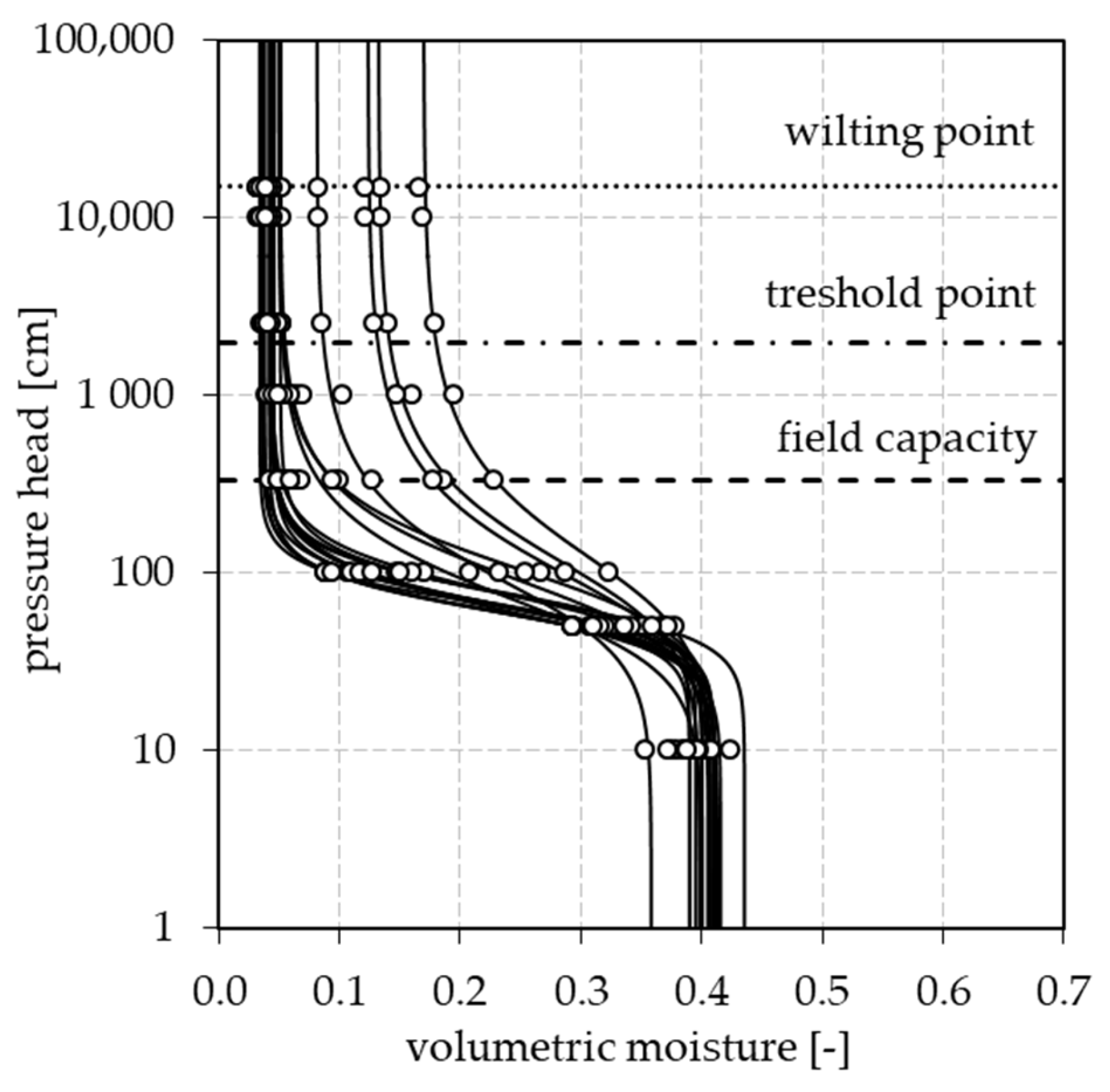
The model setting before and during the simulation corresponded to the real conditions in the lysimeter. The simulated soil profile with a thickness of 2.5 m was divided into 20 material layers. The single-pore hydraulic model without hysteresis according to van Genuchten [57], and Mualem [58], was selected. For each layer, the basic hydrophysical characteristics of soils were measured in the laboratory and the parameters of the analytical expression of moisture retention curves were defined according to van Genuchten (Figure 4 and Table 1).
In the next step, initial and boundary conditions were set. The initial humidity θ (Table 1) in the individual material layers of the soil before starting the simulation corresponded to the actual humidity in the lysimeter. The simulations were launched 1 week (168 h) ahead of the studied periods.
The time-dependent upper boundary condition was defined by hourly values of meteorological elements from the meteorological station (solar radiation, air temperature, air humidity and wind speed) and from the lysimeter (precipitation). The time-dependent lower boundary condition was defined by a constant level of GWL 1.0 m below the ground. The phenological characteristics were set constant to the height of the grass cover of 0.12 m, albedo 0.23, LAI (Leaf Area Index) 2.88 and root depth of 0.3 m.
The totals of calculated actual evapotranspiration ETa were obtained by summing the amount of water released by transpiration (from the actual root water uptake) and evaporation (from the soil surface). The Feddes reduction model [59], with parameters for grassland, was chosen for water uptake by plant roots.
2.5. Results Analysis
The correspondence between model-calculated values of evapotranspiration, water storage and flows at the bottom boundary and lysimeter-measured values was evaluated by a simple regression analysis and a series of statistical indicators:
where xm are measured values, xm_mean are average measured values, and xc are the calculated values of the investigated parameters. The root mean square error (RMSE) and relative error indices such as the Nash-Sutcliffe-Index (NS) [60], or the index of agreement (IA) [61], were used to evaluate the performance of the model. The NS index can vary in the interval (−∞, 1>. NS values between 0 and 1 can be considered as an acceptable match between measurement and calculation. If NS < 0 then the average measured value is a better predictor than the calculated value, and it is considered an unacceptable match. IA values can be between 0 and 1. A perfect match is considered when the values of indices NS and IA are close to 1 [62,63].
3. Results and Discussion
3.1. Analysis of Hourly Values of Water Balance Members
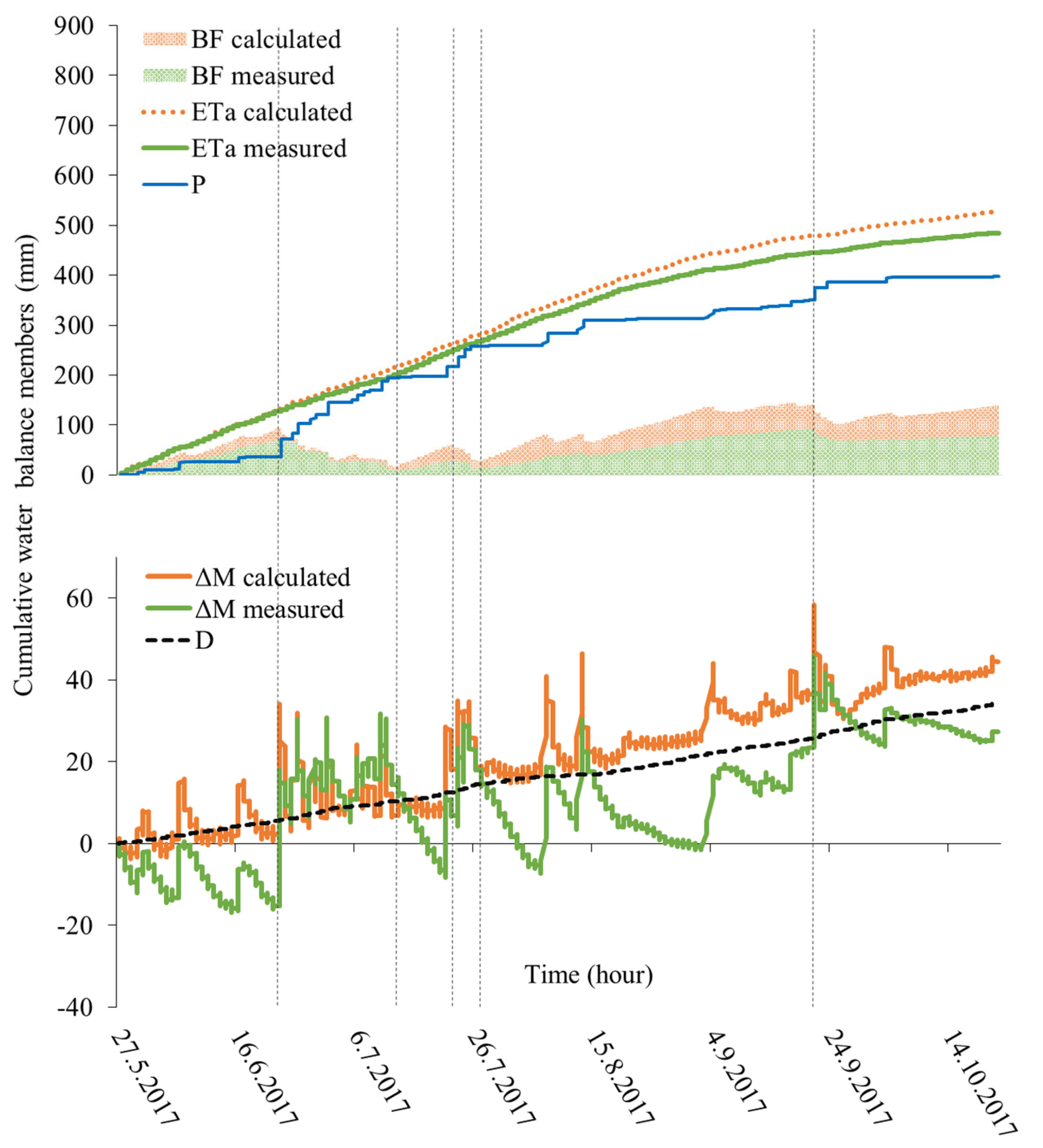
Figure 5, Figure 6 and Figure 7 show cumulative values of hourly data of individual members of the balance equation measured by a lysimeter and calculated using the HYDRUS-1D model.
Figure 5 shows the cumulative values of balance members for the period from 27 May 2017 to 21 October 2017 (148 days). From the beginning of the period until 23 June, the precipitation total was insufficient (59 mm) for the evaporation requirements. The sum of measured ETa was 130 mm and the resulting difference was eliminated by inflow (71 mm) through BF (positive BF values). The sum of calculated ETa in this period was 135 mm and BF = 92 mm. In the next period, until 13 July 2017, the opposite situation occurred. Due to the above-average rainfall (196 mm), there was enough water to maintain constant GWL, and the excess water was pumped out (−62 mm) to the measured value of BF = 9 mm. The sum of measured ETa was 200 mm and the calculated ETa was 216 mm, with a calculated BF value of 18 mm (−74 mm). The situation occurred again on 23 July 2017, when there was an inflow of water (21 mm) through BF to a value of 30 mm. In this way, the resulting deficit (−19 mm) between P (237 mm) and ETa (256 mm) was eliminated. In the case of calculated values, the deficit was higher (−32 mm) due to higher ETa (269 mm) and was eliminated by inflow (37 mm) to a value of BF = 55 mm. At the end of July, after heavy rains, water flowed from the lysimeter again (−17 mm) to BF = 13 mm. The difference between P (258 mm) and ETa (264 mm) was −6 mm, and in the case of calculated ETa (278 mm) it was −20 mm. The water outflow calculated by the model was −27 mm. The months of August and September were again below average in terms of precipitation and therefore did not provide enough water for the soil profile. The deficit between P (349 mm) and ETa (444 mm) was −95 mm and −130 mm considering the calculated ETa (479 mm). Again, water inflow (80 mm) occurred through BF = 93 mm, thus maintaining the set GWL. In the case of calculated values, the inflow was 112 mm, and BF = 140 mm. From 20 September until the end of the evaluated period, the water outflow from the lysimeter was −13 mm (BF = 79 mm) due to lower ETa totals (484 mm) in the autumn months despite below-average precipitation (398 mm).
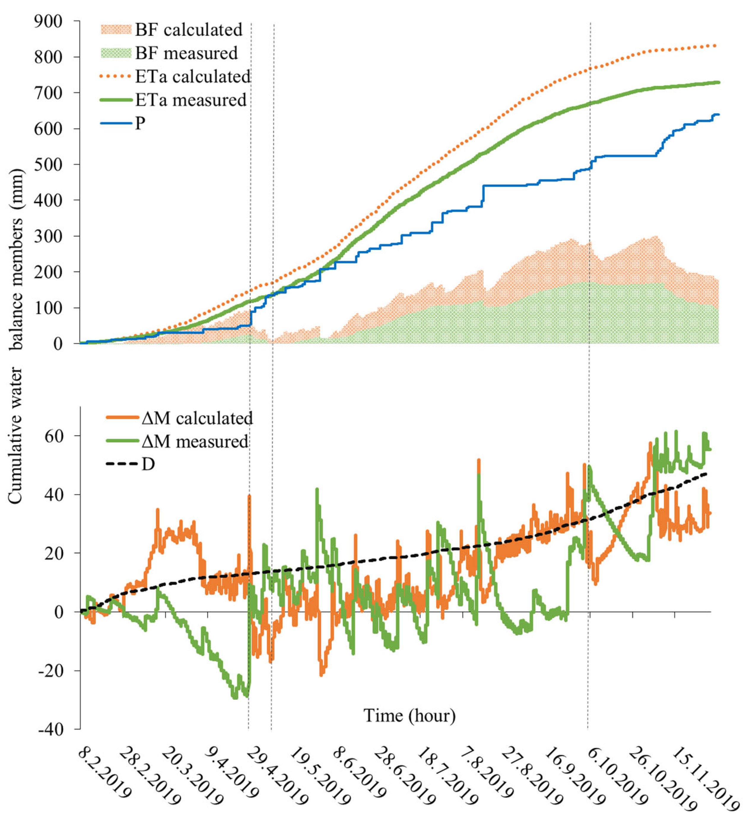
Figure 6 shows the cumulative values of the measured and calculated members of the balance equation for the period from 8 February 2019 to 30 November 2019 (296 days).
Similarly, the below-average rainfall (84 mm) from the beginning of the period until 28 April 2019 was not sufficient to keep the set GWL, and therefore it was supplied by the BF (26 mm). The sum of the measured ETa (117 mm) was lower than the calculated ETa (150 mm). The resulting difference between P and the calculated ETa (−33 mm) was eliminated by the calculated BF inflow to the level of 91 mm. The end of April to the beginning of May is characterized by the outflow of water from the profile (−27 mm) to the value BF = −1.6 mm. This was caused by lower values of ETa (134 mm), sufficiently compensated by precipitation (134 mm). The calculated ETa was higher (169 mm) and the difference between P and ETa was −35 mm. The calculated outflow was −83 mm at BF = 7.8 mm. From 7 May 2019 until 3 October 2019, the mean precipitation (508 mm) was again not sufficient to supplement the water deficit from ETa (671 mm), which was eliminated by the inflow from BF =173 mm. The total ETa in the case of calculated values was 768 mm and the difference between P and ETa was eliminated by inflow (271 mm) to the value BF = 279 mm. The exceptions were a few short periods with high above-average precipitation, during which the BF values were negative. The end of the period was characterized by the decrease in measured ETa (729 mm) and calculated ETa (832 mm), and also the water outflow decrease (−13 mm) to BF = 98 mm after smaller autumn precipitations (639 mm). The calculated outflow of −100 mm settled at the value BF = 180 mm.
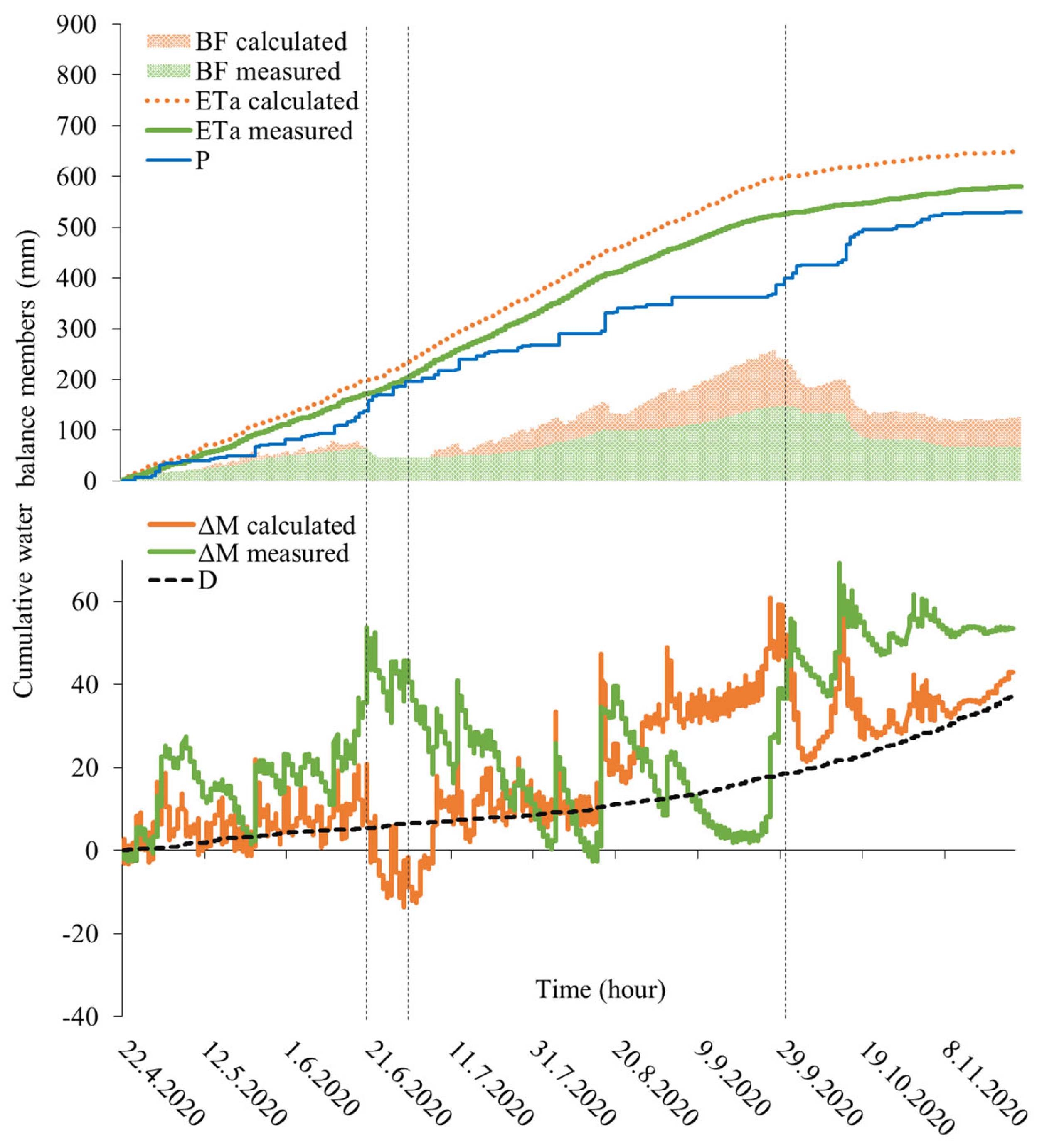
The last evaluated period in Figure 7 lasted from 22 April 2020 to 23 November 2020 (216 days).
The beginning of the period until 19 June 2020 was again average in terms of precipitation (137 mm), which was not sufficient to cover the water consumption for ETa (172 mm). This deficit was compensated by the inflow of water through the BF (65 mm). From the second half of June to the end of June, due to above-average precipitation (186 mm), water outflow (−18 mm) occurred at BF = 46 mm. The cumulative value of the measured ETa was 200 mm and the calculated ETa was 230 mm. The calculated outflow was −40 mm at BF = 26 mm. The next period until the end of September was accompanied by mostly positive BF values and thus the inflow of water into the lysimeter (102 mm) at BF = 148 mm. The difference between P (399 mm) and measured ETa (527 mm) or calculated ETa (599 mm) was compensated in the case of calculated ETa by inflow (212 mm) at BF = 239 mm. In this period, there were several short periods of heavy rainfall and short-term outflow. On the cumulative lines, it can be seen as short-term BF dips. September was dry with very low precipitation, therefore the cumulative BF line is significantly steeper. The end of the period was traditional, with few exceptions, accompanied by water outflow from the lysimeter (−80 mm) at BF = 68 mm and a decrease in measured ETa (581 mm) and calculated ETa (650 mm). The cumulative value of precipitation at the end of the period was 530 mm and the calculated outflow was −113 mm at BF = 126 mm.
Based on the cumulative evapotranspiration lines in Figure 5, Figure 6 and Figure 7, it is clear that in the investigated years, the values were balanced from the beginning of the analyzed periods until the end of summer. The highest totals of evapotranspiration were in the summer months and the lowest was in the spring and autumn months. Water regulation through BF, which compensated for losses by evaporation or excesses from precipitation, ensured that the changes in the weight of the lysimeter M were only small. Each weight change ΔM means a change in the soil water supply. By comparing the measured and calculated values, it can be concluded that the model closely follows the ETa development trends. Figure 5, Figure 6 and Figure 7 show that the model is the least reliable for calculating flows at the bottom boundary of the unsaturated zone (ΔBF) of the soil monolith. The ΔBF calculation error causes a deviation in ETa quantification by cca 11%.
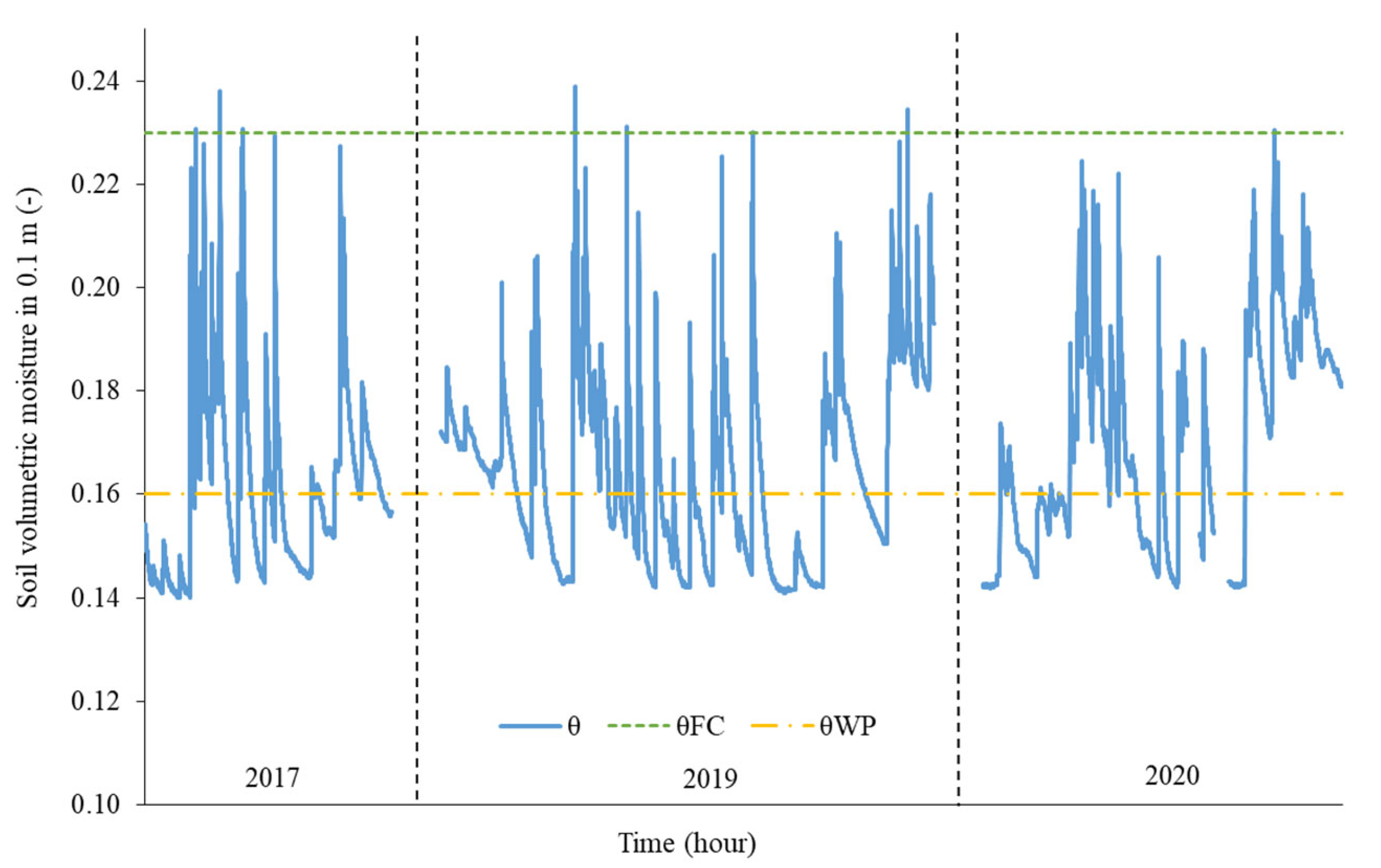
Figure 8 shows the hourly values of the measured soil volumetric moisture (θ) in the layer of 0.0–0.1 m.
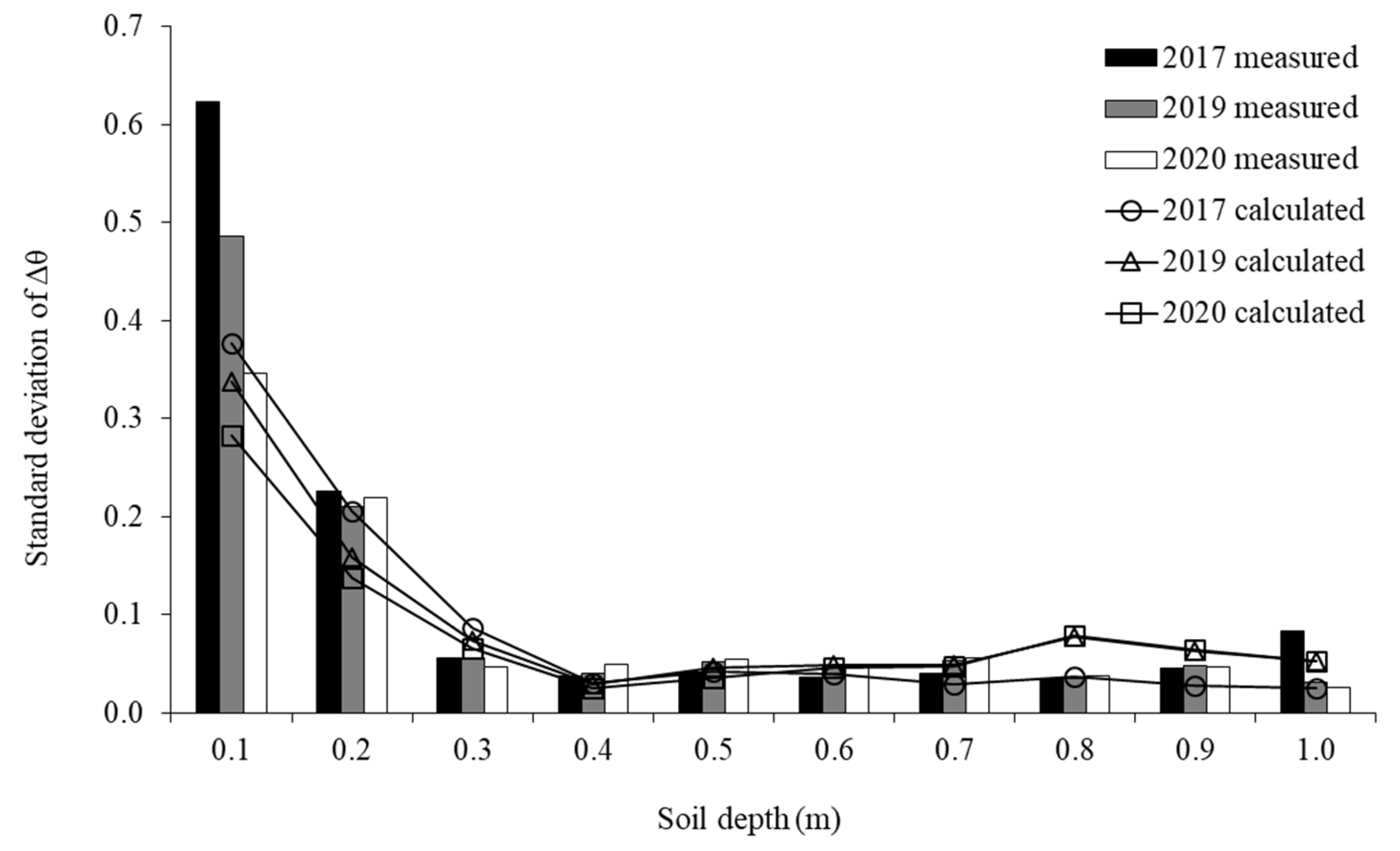
The hydrolimits of field capacity (θFC = 0.23) and wilting point (θWP = 0.16) show that the soil volumetric moisture in all evaluated periods ranged mostly between θFC and θWP. Standard deviations (SD) of hourly changes in both measured and calculated volumetric moisture (Δθ) in individual soil layers up to a depth of 1 m are shown in Figure 9.
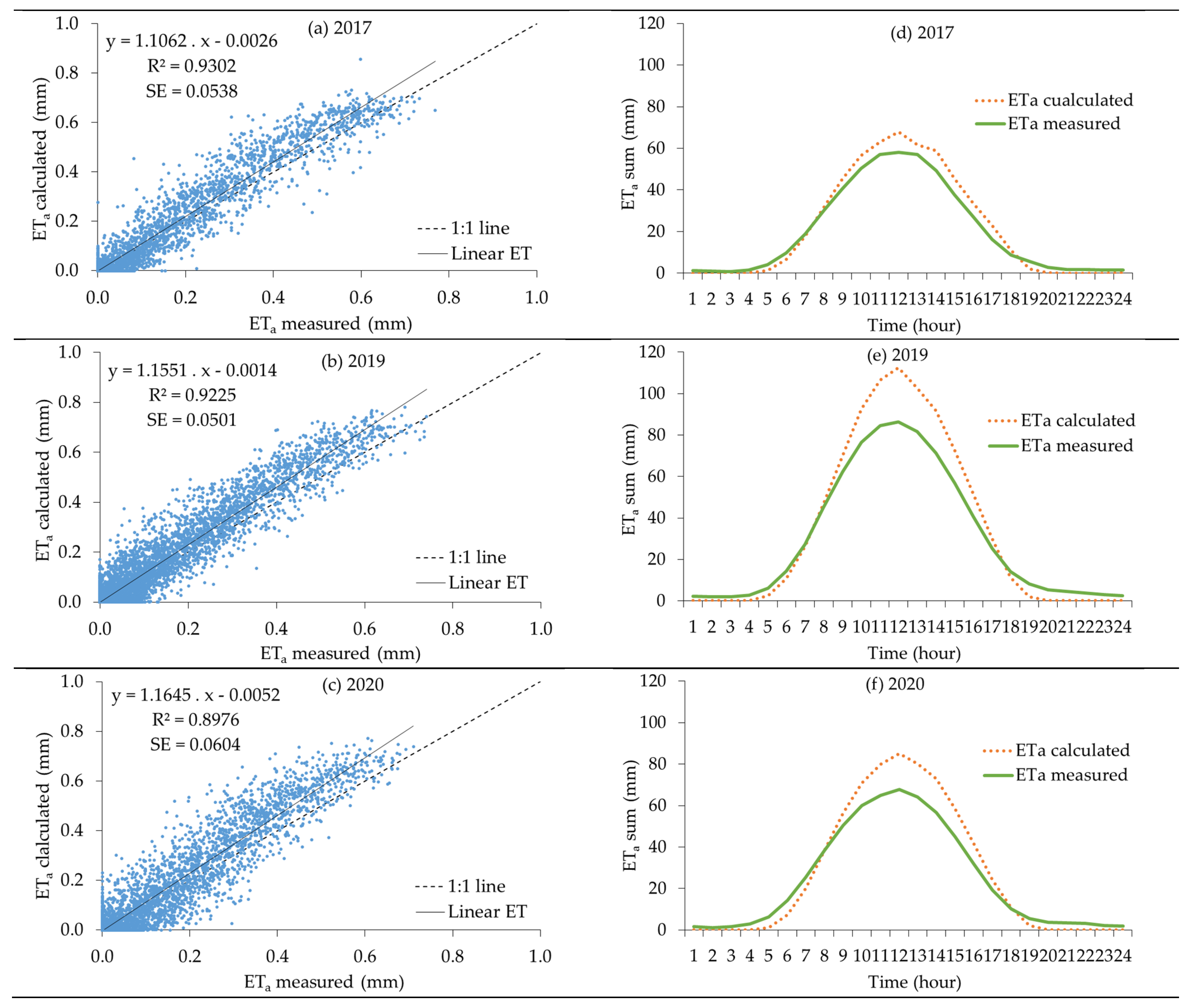
The greatest deviation Δθ from the average value occurred in the upper layers of the soil, up to 0.2 m (SD = 0.14–0.62). This is the zone of significant interaction with the atmosphere, which is most sensitive to changes in moisture caused by evapotranspiration or precipitation. The deviations in layers 0.3 to 1 m are much lower (SD = 0.02–0.09). A regression analysis of the evapotranspiration hourly totals in Figure 10a–c shows that the calculated ETa values correlate to a great extent with the measured ETa values. The values of the regression coefficients R2 (0.90–0.93) express a high degree of linear coincidence between calculation and measurement. A similar coincidence was demonstrated by lysimeter measurements, in the field, where the authors [21,22,38,64] reported regression coefficient values in the range of 0.87–0.93. Very small differences also resulted from the values of the standard error SE (0.05–0.06). The maximum hourly differences between the calculated and measured ETa in individual periods were 0.37 mm (2017), 0.32 mm (2019), and 0.35 mm (2020), and the average differences were 0.01 mm (2017) and 0.02 mm (2019 and 2020).
Figure 10d–f shows the curves of the measured and calculated ETa totals in individual hours of the day during the evaluated periods. The maximum evapotranspiration totals occurred around noon, with differences between calculated and measured ETa of 10 mm (2017), 26 mm (2019), and 17 mm (2020). The average values were identified at approximately 7 and 17 h, with differences of 1 to 7 mm.
Table 2 shows the basic statistical characteristics of the measured and calculated hourly totals of actual evapotranspiration in 2017, 2019, and 2020. The average measured hourly total of actual evapotranspiration in the investigated periods is 0.117 mm. The comparison of measured and calculated ETa totals shows that the calculated values are on average overestimated by 11%. Calculated totals have greater variability than measured ones. Both calculated and measured development evapotranspiration hourly totals are sharper compared to the normal distribution. They are skewed to the left.
3.2. Analysis of Daily Values of Water Balance Members
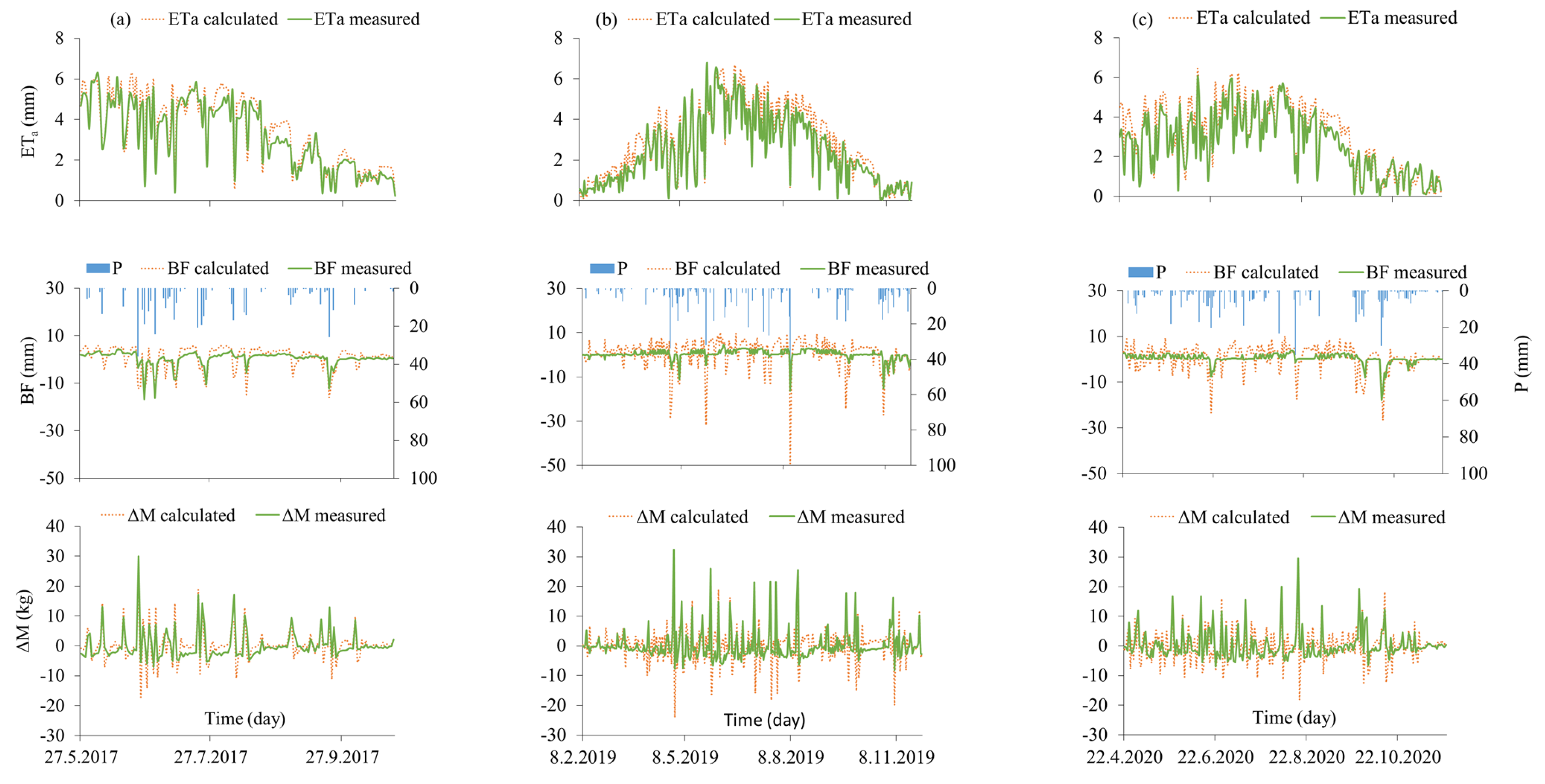
Figure 11a–c shows the daily values of the measured and calculated members of the balance equation during the analyzed years.
The performance of the model is evaluated by a series of statistical indicators expressing the rate of root mean square error (RMSE) and relative error (NS and IA) between the calculated and measured values of balance members (Table 3).
In the case of ETa, in 2017, the RMSE values were 0.51 mm, NS 0.90, and IA 0.98. In 2019, the values of the RMSE indicators were 0.53 mm, NS 0.89, and IA 0.98. In 2020, RMSE was 0.58 mm, NS was 0.86, and IA was 0.97 (Table 3). In the works of [62,65], the authors report RMSE values for evapotranspiration in the range of 0.50–0.90 mm, NS 0.35–0.75, and IA 0.85–0.94. Based on the values of statistical indicators, the performance of the model is higher compared to the results of these authors [62,65]. Other authors report NS values in the range of 0.41–0.96 and an IA of 0.93–0.99 [66,67,68]. In this case, the results fall within the upper range of the statistical indicators reported by the authors.
When evaluating the cumulative daily BF values in 2017, the RMSE were 3.30 mm, NS −0.12, and IA 0.81. In 2019, the RMSE values were 5.69 mm, NS −5.32, and IA 0.53. In the last period of 2020, the values of the indicators were as follows: RMSE 4.91 mm, NS −3.29, and IA 0.54. Based on the comparison between the RMSE values for the bottom flows BF and the results of the above-mentioned authors [62,65,66,67,68], it is obvious that the deviations of the simulated values from the measured ones are higher. These authors mentioned the RMSE values from 0.5 to 2.3 mm. In Figure 11b,c, it is clear that the calculated BF in the periods 2019 and 2020 significantly exceeded the measured values compared to 2017 (Figure 11a). However, during larger precipitation events, it is obvious that the model follows the trends well, along with the measurements. Higher differences in BF between calculation and measurement also result from NS values which are negative. When this indicator was compared with the values of other authors [62,65,66,67,68], where the NS ranged from −3.1 to 0.92, then the results approached the lower limit of the range or were even lower. A similar situation occurred with the IA indicator, where the resulting values are in the lower part of the range 0.48–0.98, as indicated by other authors [62,65,66,67,68]. The exception was the year 2017, with IA in the upper part of the range of 0.48–0.98.
The next analyzed member of the water balance is the cumulative daily values of the lysimeter weight change ΔM. In 2017, the RMSE values were 3.21 mm, NS 0.59, and IA 0.90. In 2019, the RMSE was 5.66 mm, the NS was −0.12, and the IA was 0.67. The values of the indicators for ΔM in the last period of 2020 were for RMSE 4.86 mm, NS 0.03, and IA 0.76. In all analyzed periods, the RMSE values exceeded the upper limit of the range of 1.7–2.8 mm, indicated by [65]. The comparison of the NS index with the results of other authors showed that in 2017 the value of NS was located in the upper limit of the range −1.03–0.82 indicated by other authors [57,62,65,66,68]. In 2019 and 2020, NS was located in the middle of the range. Similar results were obtained by comparing the IA index, where the values described by the authors ranged between 0.56–0.94. Again, the year 2017 was at the top of the range, and the years 2019 and 2020 were in the middle.
Table 4 shows the basic statistical characteristics of the measured and calculated daily totals of actual evapotranspiration in 2017, 2019, and 2020. The average measured daily total of actual evapotranspiration in the investigated periods is 2.81 mm. The comparison between measured and calculated ETa totals shows that, on average, the simulated values are overestimated by 11%. The calculated values have greater variability than the measured values. The calculated and measured series of evapotranspiration hourly totals are flatter with respect to the normal distribution. Both series in 2017 are skewed to the right, while in 2019 they are skewed to the left. The measured series of daily ETa totals in 2020 are skewed to the left. The calculated series of daily ETa totals in 2020 are skewed to the right.
The total values of the measured and calculated members of the water balance are described in Table 5. The differences between calculated and measured ETa in the evaluated years were 42 mm (9%—2017), 103 mm (14%—2019), and 69 mm (12%—2020).
These evapotranspiration differences caused higher values of the calculated water inflow from BF, which eliminated the resulting evapotranspiration deficit. Cumulative BF differences in the studied periods were 59 mm (2017), 82 mm (2019), and 58 mm (2020). In 2017, the calculated cumulative inflow from BF exceeded the evapotranspiration deficit, which was manifested by an increase in the calculated weight change of the lysimeter ΔM by 18 kg compared to the measurement. The opposite situation occurred in 2019 and 2020, when the calculated water inflow from BF was not sufficient to cover the evapotranspiration deficit and the calculated cumulative ΔM was lower by −21 kg (2019) and −11 kg (2020) compared to the measurement. In the case of the measured values in all evaluated periods, evapotranspiration dominated precipitation by 22% (2017), 14% (2019), and 10% (2020). The deficit was compensated by capillary inflows from the GWL and at the same time by the water supply from the unsaturated soil zone. In the soil profile, this was most evident in its upper layers.
4. Conclusions
Different time periods in 2017, 2019 and 2020 were selected for the analysis of the hourly values of the water balance members. By comparing the measured and calculated cumulative ETa totals, it was demonstrated that the results from numerical simulation slightly exceed the measured values. Higher values of the calculated ETa are caused by the dominance of the capillary inflow through BF compared to the values measured by the lysimeter. A significant increase in capillary inflow was observed during non-precipitation periods. In these periods, the inflow of water covered the need for evapotranspiration. The opposite situation occurred during periods of precipitation, when water gravitationally drained from the lysimeter into the soil saturated zone. The changes in precipitation and non-precipitation periods can be clearly seen in the course of the balance members’ cumulative values. When water inflow through BF was not sufficient to cover evapotranspiration needs, water deficit was compensated from soil water supply. This caused the decrease in the lysimeter weight ΔM. On the other hand, when BF exceeded evapotranspiration needs, the soil water supply increased and thus increased ΔM. Quantified deviations between measured and calculated values are most significant at BF, which caused smaller differences at ETa and ΔM. In general, however, it can be concluded that the model reliably simulates trends in the development of the balance members.
A regression analysis of the balance members’ daily values demonstrated a high degree of dependence between the measured and calculated ETa. Similarly, the values of the RMSE, NS, and IA evaluation indicators show a high degree of coincidence and prove good performance of the model in all evaluated years. For BF, the RMSE values were significantly higher. Worse performance of the model was demonstrated by the NS and IA indicators, which were at low values, with the exception of 2017 when the IA value was higher. A slightly better situation occurred when evaluating the ΔM indicator. In this case, although the RMSE values were high, there was also a significant increase in NS and IA in 2017, and a moderate increase in 2019 and 2020. The use of the lysimeter enabled the evaluation of the selected HYDRUS-1D model as acceptable for the conditions of the East Slovakian Lowland. In the future, it is expected that a longer time series will be used in soil water regime simulations with regard to the frequent occurrence of extreme hydrological conditions, whether they be drought or wetness.
Author Contributions
Conceptualization, B.K., A.T. and M.G.; methodology, B.K. and A.T.; software, B.K. and A.T.; validation, B.K., M.G., A.T. and D.P.; formal analysis, B.K., A.T., M.G. and D.P.; investigation, B.K.; resources, B.K, A.T. and M.G.; data curation, B.K. and A.T.; writing—original draft preparation, B.K.; writing—review and editing, B.K., M.G., A.T. and D.P.; visualization, B.K. and D.P.; supervision, B.K., A.T., M.G. and D.P.; project administration, M.G. All authors have read and agreed to the published version of the manuscript.
Funding
The authors are grateful to the Scientific Grant Agency of the Ministry of Education, Science, Re-search and Sport of the Slovak Republic: (project VEGA: 2/0044/20).
Data Availability Statement
The data used in this study are available from the corresponding author upon request.
Conflicts of Interest
The authors declare that they have no conflict of interest.
References
- Wang, H.; Zhang, M.; Cui, L.; Yu, X. Spatial Heterogeneity in Sensitivity of Evapotranspiration to Climate Change. Pol. J. Environ. Stud. 2017, 26, 2287–2293. [Google Scholar] [CrossRef] [PubMed]
- Schrader, F.; Durner, W.; Fank, J.; Gebler, S.; Pütz, T.; Hannes, M.; Wollschläger, U. Estimating Precipitation and Actual Evapotranspiration from Precision Lysimeter Measurements. Procedia Environ. Sci. 2013, 19, 543–552. [Google Scholar] [CrossRef] [Green Version]
- Allen, R.G.; Tasumi, M.; Trezza, R. Benefits from Tying Satellite-Based Energy Balance to Reference Evapotranspiration. AIP Conf. Proc. 2006, 852, 127–137. [Google Scholar] [CrossRef]
- Tuttobene, R.; Vagliasindi, C. Biomass accumulation and its relationship with evapotranspiration on durum wheat (Akumulace biomasy a její vztah k evapotranspiraci u tvrdé pšenice). In Third Congress of the European Society for Agronomy. Padova University, 18–22 September 1994; Borin, M., Sattin, M., Eds.; ESA: Paris, France, 1995; pp. 262–263. [Google Scholar]
- Novák, V. Soil-Plant-Atmosphere System. In Evapotranspiration in the Soil-Plant-Atmosphere System; Novák, V., Ed.; Progress in Soil Science; Springer: Dordrecht, The Netherlands, 2012; pp. 15–24. [Google Scholar] [CrossRef]
- Liu, X.; Liu, C.; Liu, X.; Li, C.; Cai, L.; Dong, M. Spatial and Temporal Variation in Reference Evapotranspiration and Its Climatic Drivers in Northeast China. Water 2022, 14, 3911. [Google Scholar] [CrossRef]
- Food and Agriculture Organization of the United Nations. Expert Consultation on Revision of FAO Methodologies for Crop Water Requirements; Annex, V., Ed.; FAO Penman-Monteith Formula: Rome, Italy, 1990. [Google Scholar]
- Allen, R.; Pereira, L.; Smith, M. Crop Evapotranspiration-Guidelines for Computing Crop Water Requirements-FAO Irrigation and Drainage Paper 56; FAO: Rome, Italy, 1998; Volume 56. [Google Scholar]
- Allen, R.G.; Walter, I.A.; Elliot, R.L.; Howell, T.A.; Intenfisu, D.; Jensen, M.E.; Snyder, R.L. The ASCE Standardized Reference Evapotranspiration Equation; American Society of Civil Engineers: Reston, VA, USA, 2005; 216p. [Google Scholar] [CrossRef]
- Pereira, L.S.; Allen, R.G.; Smith, M.; Raes, D. Crop Evapotranspiration Estimation with FAO56: Past and Future. Agric. Water Manag. 2015, 147, 4–20. [Google Scholar] [CrossRef]
- Penman, H.L.; Keen, B.A. Natural Evaporation from Open Water, Bare Soil and Grass. Proc. R. Soc. Lond. Ser. A. Math. Phys. Sci. 1948, 193, 120–145. [Google Scholar] [CrossRef] [Green Version]
- Monteith, J.L. Evaporation and Environment. Symp. Soc. Exp. Biol. 1965, 19, 205–234. [Google Scholar]
- Monteith, J.L. Evaporation and Surface Temperature. Q. J. R. Meteorol. Soc. 1981, 107, 1–27. [Google Scholar] [CrossRef]
- Monteith, J.L.; Unsworth, M.H. Principles of Environmental Physics; Edward Arnold: London, UK, 1990. [Google Scholar]
- Walter, I.A.; Allen, R.; Elliott, R.; Jensen, M.; Itenfisu, D.; Howell, T.; Snyder, R.L.; Brown, P.; Echings, S. The ASCE Standardized Reference Evapotranspiration Equation. Final Rep. Task Comm. Stand. Ref. Evapotranspiration 2001, 70. [Google Scholar] [CrossRef]
- Djaman, K.; Irmak, S.; Sall, M.; Sow, A.; Kabenge, I. Comparison of Sum-of-Hourly and Daily Time Step Standardized ASCE Penman-Monteith Reference Evapotranspiration. Theor. Appl. Clim. 2018, 134, 533–543. [Google Scholar] [CrossRef]
- Cai, J.; Liu, Y.; Lei, T.; Pereira, L.S. Estimating Reference Evapotranspiration with the FAO Penman–Monteith Equation Using Daily Weather Forecast Messages. Agric. For. Meteorol. 2007, 145, 22–35. [Google Scholar] [CrossRef]
- He, Q.-L.; Xiao, J.-L.; Shi, W.-Y. Responses of Terrestrial Evapotranspiration to Extreme Drought: A Review. Water 2022, 14, 3847. [Google Scholar] [CrossRef]
- Abtew, W. Evapotranspiration Measurements and Modeling for Three Wetland Systems in South Florida1. JAWRA J. Am. Water Resour. Assoc. 1996, 32, 465–473. [Google Scholar] [CrossRef]
- Feltrin, R.M.; de Paiva, J.B.D.; de Paiva, E.M.C.D.; Meissner, R.; Rupp, H.; Borg, H. Use of Lysimeters to Assess Water Balance Components in Grassland and Atlantic Forest in Southern Brazil. Water Air Soil Pollut. 2017, 228, 247. [Google Scholar] [CrossRef]
- Xu, C.-Y.; Chen, D. Comparison of seven models for estimation of evapotranspiration and groundwater recharge using lysimeter measurement data in Germany. Hydrol. Process. 2005, 19, 3717–3734. [Google Scholar] [CrossRef]
- Todorovic, M. Single-Layer Evapotranspiration Model with Variable Canopy Resistance. J. Irrig. Drain. Eng. 1999, 125, 235–245. [Google Scholar] [CrossRef]
- Vitková, J.; Šurda, P.; Zvala, A. Changes in soil moisture values two years after biochar reapplication. Acta Hydrol. Slovaca 2020, 21, 133–138. [Google Scholar] [CrossRef]
- Gombos, M. Water Storage Dependability in Root Zone of Soil. Cereal Res. Commun. 2008, 36, 1191–1194. [Google Scholar]
- Gomboš, M.; Kandra, B.; Tall, A.; Pavelková, D. The Role of Evaporation in the Drying of a Soil Profile. Adv. Therm. Process. Energy Transform. 2020, 3, 45–52. [Google Scholar] [CrossRef]
- Sarma, A.; Bharadwaj, K. Determination of Crop-Coefficients and Estimation of Evapotranspiration of Rapeseed Using Lysimeter and Different Reference Evapotranspiration Models. J. Agrometeorol. 2020, 22, 172–178. [Google Scholar] [CrossRef]
- Liu, X.; Xu, C.; Zhong, X.; Li, Y.; Yuan, X.; Cao, J. Comparison of 16 Models for Reference Crop Evapotranspiration against Weighing Lysimeter Measurement. Agric. Water Manag. 2017, 184, 145–155. [Google Scholar] [CrossRef]
- Barek, V.; Halaj, P.; Zembery, J.; Barekova, A.; Halajova, D. Modern management methods in microorrigation use. In Proceedings of the International Multidisciplinary Scientific GeoConference: SGEM Surveying Geology & Mining Ecology Management Sofia, Albena, Bulgaria, 16–22 June 2013; pp. 221–228. [Google Scholar]
- Cui, Y.; Ning, S.; Jin, J.; Jiang, S.; Zhou, Y.; Wu, C. Quantitative Lasting Effects of Drought Stress at a Growth Stage on Soybean Evapotranspiration and Aboveground BIOMASS. Water 2021, 13, 18. [Google Scholar] [CrossRef]
- Grodzka-Łukaszewska, M.; Sinicyn, G.; Grygoruk, M.; Mirosław-Świątek, D.; Kardel, I.; Okruszko, T. The Role of the River in the Functioning of Marginal Fen: A Case Study from the Biebrza Wetlands. PeerJ 2022, 10, e13418. [Google Scholar] [CrossRef] [PubMed]
- Meissner, R.; Rupp, H.; Haselow, L. Chapter 7—Use of Lysimeters for Monitoring Soil Water Balance Parameters and Nutrient Leaching. In Climate Change and Soil Interactions; Prasad, M.N.V., Pietrzykowski, M., Eds.; Elsevier: Amsterdam, The Netherlands, 2020; pp. 171–205. [Google Scholar] [CrossRef]
- Brown, S.; Wagner-Riddle, C.; Debruyn, Z.; Jordan, S.; Berg, A.; Ambadan, J.T.; Congreves, K.A.; Machado, P.V.F. Assessing Variability of Soil Water Balance Components Measured at a New Lysimeter Facility Dedicated to the Study of Soil Ecosystem Services. J. Hydrol. 2021, 603, 127037. [Google Scholar] [CrossRef]
- Doležal, F.; Hernandez-Gomis, R.; Matula, S.; Gulamov, M.; Miháliková, M.; Khodjaev, S. Actual Evapotranspiration of Unirrigated Grass in a Smart Field Lysimeter. Vadose Zone J. 2018, 17, 170173. [Google Scholar] [CrossRef]
- Bochníček, O.; Hrušková, K. Climate Atlas of Slovakia; Slovak Hydrometeorological Institute: Banská Bystrica, Slovakia, 2015; 131p, ISBN 978-0-8412-3999-9. [Google Scholar]
- Documentation Lysimeter Station Michalovce. Groundwater Principle Michalovce. Umwelt-Geräte-Technik GmbH: Müncheberg. 2014. Available online: http://www.ugt-online.de (accessed on 1 May 2014).
- Gombos, M.; Tall, A.; Kandra, B.; Pavelková, D. Influence of Soil Type on Statistical Characteristics and Graphical Results Interpretation of the Water Storage Distribution Monitoring along the Vertical of the Soil Profile. Acta Hydrol. Slovaca 2021, 22, 97–105. [Google Scholar] [CrossRef]
- Ramier, D.; Berthier, E.; Andrieu, H. An Urban Lysimeter to Assess Runoff Losses on Asphalt Concrete Plates. Phys. Chem. Earth Parts A/B/C 2004, 29, 839–847. [Google Scholar] [CrossRef]
- Vaughan, P.J.; Trout, T.J.; Ayars, J.E. A Processing Method for Weighing Lysimeter Data and Comparison to Micrometeorological ETo Predictions. Agric. Water Manag. 2007, 88, 141–146. [Google Scholar] [CrossRef]
- Peters, A.; Nehls, T.; Schonsky, H.; Wessolek, G. Separating Precipitation and Evapotranspiration from Noise—A New Filter Routine for High-Resolution Lysimeter Data. Hydrol. Earth Syst. Sci. 2014, 18, 1189–1198. [Google Scholar] [CrossRef]
- Nolz, R. A Review on the Quantification of Soil Water Balance Components as a Basis for Agricultural Water Management with a Focus on Weighing Lysimeters and Soil Water Sensors/Ein Überblick Über Die Ermittlung von Wasserhaushaltsgrößen Als Basis Für Die Landeskulturelle Wasserwirtschaft Mit Fokus Auf Lysimeter Und Bodenwassersensoren. Bodenkult. J. Land Manag. Food Environ. 2016, 67, 133–144. [Google Scholar] [CrossRef] [Green Version]
- Gebler, S.; Hendricks Franssen, H.-J.; Pütz, T.; Post, H.; Schmidt, M.; Vereecken, H. Actual Evapotranspiration and Precipitation Measured by Lysimeters: A Comparison with Eddy Covariance and Tipping Bucket. Hydrol. Earth Syst. Sci. 2015, 19, 2145–2161. [Google Scholar] [CrossRef] [Green Version]
- Bethge-Steffens, D.; Meissner, R.; Rupp, H. Development and Practical Test of a Weighable Groundwater Lysimeter for Floodplain Sites. J. Plant Nutr. Soil Sci. 2004, 167, 516–524. [Google Scholar] [CrossRef]
- Tall, A.; Pavelková, D. Results of Water Balance Measurements in a Sandy and Silty-Loam Soil Profile Using Lysimeters. J. Water Land Dev. 2020, 45, 179–184. [Google Scholar] [CrossRef]
- Feltrin, R.M.; de Paiva, J.B.D.; de Paiva, E.M.C.D.; Beling, F.A. Lysimeter Soil Water Balance Evaluation for an Experiment Developed in the Southern Brazilian Atlantic Forest Region. Hydrol. Process. 2011, 25, 2321–2328. [Google Scholar] [CrossRef]
- Evett, S.R.; Schwartz, R.C.; Howell, T.A.; Louis Baumhardt, R.; Copeland, K.S. Can Weighing Lysimeter ET Represent Surrounding Field ET Well Enough to Test Flux Station Measurements of Daily and Sub-Daily ET? Adv. Water Resour. 2012, 50, 79–90. [Google Scholar] [CrossRef]
- Nolz, R.; Cepuder, P.; Kammerer, G. Determining Soil Water-Balance Components Using an Irrigated Grass Lysimeter in NE Austria. J. Plant Nutr. Soil Sci. 2014, 177, 237–244. [Google Scholar] [CrossRef]
- Tall, A. Impact of Canopy on the Water Storage Dynamics in Soil. Cereal Res. Commun. 2007, 35, 1185–1188. [Google Scholar] [CrossRef]
- Tall, A. Application of the Palmer Drought Severity Index in East Slovakian Lowland. Cereal Res. Commun. 2008, 36, 1195–1198. [Google Scholar]
- Kandra, B.; Gomboš, M. Influence of Climatic Elements on the Water Regime in a Soil Profile. Cereal Res. Commun. 2008, 36, 1187–1190. [Google Scholar]
- Rončák, P.; Šurda, P.; Vitková, J. Analysis of a Topsoil Moisture Regime through an Effective Precipitation Index for the Locality of Nitra, Slovakia. Slovak J. Civ. Eng. 2021, 29, 9–14. [Google Scholar] [CrossRef]
- Sleziak, P.; Szolgay, J.; Hlavčová, K.; Parajka, J. The Impact of the Variability of Precipitation and Temperatures on the Efficiency of a Conceptual Rainfall-Runoff Model. Slovak J. Civ. Eng. 2016, 24, 1–7. [Google Scholar] [CrossRef]
- Gomboš, M.; Pavelková, D.; Kandra, B.; Tall, A. Impact of Soil Texture and Position of Groundwater Level on Evaporation from the Soil Root Zone. In Water Resources in Slovakia: Part I: Assessment and Development; Negm, A.M., Zeleňáková, M., Eds.; The Handbook of Environmental Chemistry; Springer International Publishing: Cham, Switzerland, 2019; pp. 167–181. [Google Scholar] [CrossRef]
- Šoltész, A.; Baroková, D.; Červeňaská, M.; Janík, A. Hydrodynamic analysis of interaction between river flow and ground water. In Proceedings of the 16th International Multidisciplinary Scientific GeoConference SGEM 2016, Albena, Bulgaria, 28 June–6 July 2016; pp. 823–830. [Google Scholar]
- Kowalik, P.J. Drainage and Capillary Rise Components in Water Balance of Alluvial Soils. Agric. Water Manag. 2006, 86, 206–211. [Google Scholar] [CrossRef]
- Groh, J.; Slawitsch, V.; Herndl, M.; Graf, A.; Vereecken, H.; Pütz, T. Determining Dew and Hoar Frost Formation for a Low Mountain Range and Alpine Grassland Site by Weighable Lysimeter. J. Hydrol. 2018, 563, 372–381. [Google Scholar] [CrossRef]
- Šimůnek, J.; Jirka; Saito, H.; Sakai, M.; Van Genuchten, M. The HYDRUS-1D Software Package for Simulating the One-Dimensional Movement of Water, Heat, and Multiple Solutes in Variably-Saturated Media; University of California: Riverside, CA, USA, 2008. [Google Scholar]
- van Genuchten, M.T. A Closed-Form Equation for Predicting the Hydraulic Conductivity of Unsaturated Soils. Soil Sci. Soc. Am. J. 1980, 44, 892–898. [Google Scholar] [CrossRef] [Green Version]
- Mualem, Y. A New Model for Predicting the Hydraulic Conductivity of Unsaturated Porous Media. Water Resour. Res. 1976, 12, 513–522. [Google Scholar] [CrossRef] [Green Version]
- Feddes, R.A.; Kowalik, P.J.; Zaradny, H. Simulation of Field Water Use and Crop Yield; John Wiley & Sons: New York, NY, USA, 1978. [Google Scholar]
- Nash, J.E.; Sutcliffe, J.V. River Flow Forecasting through Conceptual Models Part I—A Discussion of Principles. J. Hydrol. 1970, 10, 282–290. [Google Scholar] [CrossRef]
- Willmott, C.J. Some Comments on the Evaluation of Model Performance. Bull. Am. Meteorol. Soc. 1982, 63, 1309–1313. [Google Scholar] [CrossRef]
- Wegehenkel, M.; Gerke, H.H. Comparison of Real Evapotranspiration Measured by Weighing Lysimeters with Simulations Based on the Penman Formula and a Crop Growth Model. J. Hydrol. Hydromech. 2013, 61, 161–172. [Google Scholar] [CrossRef] [Green Version]
- Moriasi, D.; Arnold, J.; Van Liew, M.; Bingner, R.; Harmel, R.D.; Veith, T. Model Evaluation Guidelines for Systematic Quantification of Accuracy in Watershed Simulations. Trans. ASABE 2007, 50, 885–900. [Google Scholar] [CrossRef]
- Nolz, R.; Cepuder, P.; Eitzinger, J. Comparison of Lysimeter Based and Calculated ASCE Reference Evapotranspiration in a Subhumid Climate. Theor. Appl. Clim. 2016, 124, 315–324. [Google Scholar] [CrossRef]
- Wegehenkel, M.; Gerke, H.H. Water table effects on measured and simulated fluxes in weighing lysimeters for differently-textured soils. J. Hydrol. Hydromech. 2015, 63, 82–92. [Google Scholar] [CrossRef] [Green Version]
- Luo, Y.; Sophocleous, M. Seasonal Groundwater Contribution to Crop-Water Use Assessed with Lysimeter Observations and Model Simulations. J. Hydrol. 2010, 389, 325–335. [Google Scholar] [CrossRef]
- Loos, C.; Gayler, S.; Priesack, E. Assessment of Water Balance Simulations for Large-Scale Weighing Lysimeters. J. Hydrol. 2007, 335, 259–270. [Google Scholar] [CrossRef]
- Herbst, M.; Fialkiewicz, W.; Chen, T.; Pütz, T.; Thiéry, D.; Mouvet, C.; Vachaud, G.; Vereecken, H. Intercomparison of Flow and Transport Models Applied to Vertical Drainage in Cropped Lysimeters. Vadose Zone J. 2005, 4, 354–359. [Google Scholar] [CrossRef]
Figure 1.
The location of (a) the lysimeter station, and (b) the soil monolith sample point.

Figure 2.
Lysimetric station in the Petrovce nad Laborcom with lysimeter function design.

Figure 3.
Identification of (a) soil types according to USDA and (b) soil texture along the vertical line of the soil profile.
Figure 3.
Identification of (a) soil types according to USDA and (b) soil texture along the vertical line of the soil profile.

Figure 4.
Measured values (white circles) of moisture retention curves and their analytical expressions according to van Genuchten’s parameters.
Figure 4.
Measured values (white circles) of moisture retention curves and their analytical expressions according to van Genuchten’s parameters.

Figure 5.
Cumulative hourly values of water balance members for the period 2017.

Figure 6.
Cumulative hourly values of water balance members for the 2019.

Figure 7.
Cumulative hourly values of water balance members for the period 2020.

Figure 8.
Soil volumetric moisture measured in the 0.0–0.1 m layer with hydrolimits for the periods 2017, 2019 and 2020.
Figure 8.
Soil volumetric moisture measured in the 0.0–0.1 m layer with hydrolimits for the periods 2017, 2019 and 2020.

Figure 9.
Standard deviations of the measured and calculated hourly changes in soil volumetric moisture (Δθ) in individual soil layers for the periods 2017, 2019 and 2020.
Figure 9.
Standard deviations of the measured and calculated hourly changes in soil volumetric moisture (Δθ) in individual soil layers for the periods 2017, 2019 and 2020.

Figure 10.
Regression analysis and hourly sums of measured and calculated evapotranspiration for the periods (a,d) 2017, (b,e) 2019, and (c,f) 2020.
Figure 10.
Regression analysis and hourly sums of measured and calculated evapotranspiration for the periods (a,d) 2017, (b,e) 2019, and (c,f) 2020.

Figure 11.
Daily values of the measured and calculated water balance members for the periods (a) 2017, (b) 2019, and (c) 2020.
Figure 11.
Daily values of the measured and calculated water balance members for the periods (a) 2017, (b) 2019, and (c) 2020.


Table 1.
Parameters of the analytical expression of soil moisture retention curves for soil in a lysimeter.
Table 1.
Parameters of the analytical expression of soil moisture retention curves for soil in a lysimeter.
| Soil Depth (m) | θr (-) | θsH (-) | α (1/mm) | n (-) | Ks (mm/h) | θ (-) |
|---|---|---|---|---|---|---|
| 0.0–0.1 | 0.1697 | 0.4070 | 0.0012 | 2.0045 | 3.5 | 0.2409 |
| 0.1–0.2 | 0.1323 | 0.3984 | 0.0012 | 2.0639 | 14.0 | 0.2600 |
| 0.2–0.3 | 0.1236 | 0.4137 | 0.0014 | 2.0711 | 20.6 | 0.2791 |
| 0.3–0.4 | 0.0813 | 0.3583 | 0.0015 | 2.1563 | 56.3 | 0.2981 |
| 0.4–0.5 | 0.0434 | 0.3952 | 0.0013 | 4.2317 | 170.7 | 0.3172 |
| 0.5–0.6 | 0.0452 | 0.4005 | 0.0014 | 4.0877 | 139.4 | 0.3362 |
| 0.6–0.7 | 0.0338 | 0.3901 | 0.0016 | 4.8526 | 282.7 | 0.3553 |
| 0.7–0.8 | 0.0417 | 0.4001 | 0.0018 | 4.3320 | 353.0 | 0.3743 |
| 0.8–0.9 | 0.0494 | 0.3991 | 0.0018 | 2.2947 | 168.4 | 0.3934 |
| 0.9–1.0 | 0.0504 | 0.4124 | 0.0012 | 2.5028 | 153.2 | 0.4124 |
| 1.0–1.1 | 0.0509 | 0.4065 | 0.0014 | 2.3620 | 188.6 | 0.4065 |
| 1.1–1.2 | 0.0427 | 0.4157 | 0.0018 | 3.3382 | 262.0 | 0.4157 |
| 1.2–1.3 | 0.0355 | 0.4052 | 0.0018 | 4.1204 | 297.1 | 0.4052 |
| 1.3–1.4 | 0.0374 | 0.4103 | 0.0016 | 4.0773 | 332.3 | 0.4103 |
| 1.4–1.5 | 0.0441 | 0.4108 | 0.0015 | 3.4231 | 244.5 | 0.4108 |
| 1.5–1.6 | 0.0509 | 0.4356 | 0.0015 | 3.8395 | 267.4 | 0.4356 |
| 1.6–1.7 | 0.0455 | 0.4102 | 0.0016 | 4.2176 | 330.5 | 0.4102 |
| 1.7–1.8 | 0.0451 | 0.4104 | 0.0017 | 3.7318 | 367.1 | 0.4104 |
| 1.8–1.9 | 0.0376 | 0.3902 | 0.0017 | 4.2901 | 372.4 | 0.3902 |
| 1.9–2.5 | 0.0504 | 0.4124 | 0.0012 | 2.5028 | 311.7 | 0.4075 |
Table 2.
Descriptive statistics of the measured and calculated hourly totals of actual evapotranspiration.
Table 2.
Descriptive statistics of the measured and calculated hourly totals of actual evapotranspiration.
| Statistical Indicator | 2017 | 2019 | 2020 | |||
|---|---|---|---|---|---|---|
| ETa | ETa * | ETa | ETa * | ETa | ETa * | |
| Mean | 0.136 | 0.148 | 0.103 | 0.117 | 0.112 | 0.125 |
| Median | 0.046 | 0.027 | 0.030 | 0.011 | 0.032 | 0.011 |
| Standard Deviation | 0.177 | 0.204 | 0.150 | 0.180 | 0.154 | 0.189 |
| Kurtosis | 0.764 | 0.226 | 2.330 | 1.593 | 1.353 | 1.016 |
| Skewness | 1.350 | 1.240 | 1.749 | 1.614 | 1.500 | 1.486 |
| Range | 0.769 | 0.855 | 0.740 | 0.781 | 0.711 | 0.772 |
| Minimum | 0.000 | 0.000 | 0.000 | 0.000 | 0.000 | 0.000 |
| Maximum | 0.769 | 0.855 | 0.740 | 0.781 | 0.711 | 0.772 |
| Count | 3552.000 | 3552.000 | 7104.000 | 7104.000 | 5184.000 | 5184.000 |
* Calculated values.
Table 3.
Values of statistical indicators between the calculated and measured members of the water balance.
Table 3.
Values of statistical indicators between the calculated and measured members of the water balance.
| 2017 | 2019 | 2020 | |||||||
|---|---|---|---|---|---|---|---|---|---|
| ETa | BF | ΔM | ETa | BF | ΔW | ETa | BF | ΔM | |
| RMSE | 0.51 | 3.30 | 3.21 | 0.53 | 5.69 | 5.66 | 0.58 | 4.91 | 4.86 |
| NS | 0.90 | −0.12 | 0.59 | 0.89 | −5.32 | −0.12 | 0.86 | −3.29 | 0.03 |
| IA | 0.98 | 0.81 | 0.90 | 0.98 | 0.53 | 0.67 | 0.97 | 0.54 | 0.76 |
Table 4.
Descriptive statistics of the measured and calculated daily totals of actual evapotranspiration.
Table 4.
Descriptive statistics of the measured and calculated daily totals of actual evapotranspiration.
| Statistical Indicator | 2017 | 2019 | 2020 | |||
|---|---|---|---|---|---|---|
| ETa | ETa * | ETa | ETa * | ETa | ETa * | |
| Mean | 3.271 | 3.555 | 2.462 | 2.811 | 2.689 | 3.008 |
| Median | 3.176 | 3.795 | 2.168 | 2.730 | 2.860 | 3.326 |
| Standard Deviation | 1.651 | 1.692 | 1.643 | 1.761 | 1.525 | 1.728 |
| Kurtosis | −1.344 | −1.317 | −0.780 | −1.017 | −0.956 | −1.214 |
| Skewness | −0.099 | −0.164 | 0.479 | 0.247 | 0.054 | −0.141 |
| Range | 6.036 | 5.966 | 6.778 | 6.599 | 5.987 | 6.354 |
| Minimum | 0.249 | 0.351 | 0.032 | 0.058 | 0.012 | 0.068 |
| Maximum | 6.285 | 6.317 | 6.809 | 6.657 | 5.999 | 6.422 |
| Count | 148.000 | 148.000 | 296.000 | 296.000 | 216.000 | 216.000 |
* Calculated values.
Table 5.
Sums of measured and calculated water balance members in the periods 2017, 2019, and 2020.
| Year | Days | ΣP (mm) | ΣD (mm) | ΣCR (mm) | ΣCR * (mm) | ΣETa (mm) | ΣETa * (mm) | ΣETa–ΣETa * (mm) |
|---|---|---|---|---|---|---|---|---|
| 2017 | 148 | 398 | 34 | 188 | 363 | 484 | 526 | −40 |
| 2019 | 296 | 639 | 48 | 239 | 742 | 729 | 832 | −103 |
| 2020 | 216 | 530 | 37 | 170 | 506 | 581 | 650 | −69 |
| Year | Days | ΣSW (mm) | ΣSW * (mm) | ΣBF (mm) | ΣBF * (mm) | ΣΔM (kg) | ΣΔM * (kg) | ΣΔM–ΔM * (mm) |
| 2017 | 148 | −109 | −225 | 79 | 138 | 27 | 45 | −18 |
| 2019 | 296 | −142 | −563 | 98 | 179 | 55 | 34 | 21 |
| 2020 | 216 | −102 | −380 | 68 | 126 | 54 | 43 | 11 |
* Calculated values.
Disclaimer/Publisher’s Note: The statements, opinions and data contained in all publications are solely those of the individual author(s) and contributor(s) and not of MDPI and/or the editor(s). MDPI and/or the editor(s) disclaim responsibility for any injury to people or property resulting from any ideas, methods, instructions or products referred to in the content. |
© 2023 by the authors. Licensee MDPI, Basel, Switzerland. This article is an open access article distributed under the terms and conditions of the Creative Commons Attribution (CC BY) license (https://creativecommons.org/licenses/by/4.0/).
Share and Cite
MDPI and ACS Style
Kandra, B.; Tall, A.; Gomboš, M.; Pavelková, D. Quantification of Evapotranspiration by Calculations and Measurements Using a Lysimeter. Water 2023, 15, 373. https://doi.org/10.3390/w15020373
AMA Style
Kandra B, Tall A, Gomboš M, Pavelková D. Quantification of Evapotranspiration by Calculations and Measurements Using a Lysimeter. Water. 2023; 15(2):373. https://doi.org/10.3390/w15020373
Chicago/Turabian StyleKandra, Branislav, Andrej Tall, Milan Gomboš, and Dana Pavelková. 2023. "Quantification of Evapotranspiration by Calculations and Measurements Using a Lysimeter" Water 15, no. 2: 373. https://doi.org/10.3390/w15020373
Note that from the first issue of 2016, this journal uses article numbers instead of page numbers. See further details here.