On the Precipitation Trends in Global Major Metropolitan Cities under Extreme Climatic Conditions: An Analysis of Shifting Patterns

Abstract

On a local and regional level, climate change has had a significant impact on precipitation in the global climatic state. The purpose of this research is to examine the trend and character of urban precipitation in the world’s most densely inhabited metropolis. From 1981 to 2020, 40 years of monthly and annual precipitation data from 50 major metropolitan cities throughout the world, based on population statistics, were analysed. The monthly and annual precipitation analysis was done using a homogeneity test, shifting point test, non-parametric Modified Mann Kendall test, and also through computing the magnitude of the trend using Sen’s slope estimate. According to the findings of the study, the most homogeneous data was obtained in May (90 %) and the least in September (74%). In 2002, the highest number of breakpoints were found in July (9 cities) and August (8 cities). The month of January has the largest significant positive trend (10 cities) whereas annually it has 20 cities. The monthly maximum of the significant negative trend was discovered in February (4 cities) and annually in 2 main cities. In November, the maximum positive and minimum positive Sen’s slope values were found to be 82% and 56%, respectively. The findings of this study are important for future water resource projections, flood or drought predictions, and engineering, scientific, industrial, agricultural, and social studies. The goal of this research is to come up with a good plan for dealing with urban flash floods and droughts as precipitation acts as the key parameter of the hydrological cycle.

1. Introduction

Precipitation is an important component of the world hydrological cycle because it aids socio-economic development [1,2]. Rainfall precipitation replenishes Earth’s freshwater resources, which are the primary source of fresh water. Obtaining proper watershed planning and management requires rainfall duration, time, and accurate information [3], and proposing plans to cope with floods and drought conditions too [4,5]. Rainfall is vital for agriculture to cultivate crops for future food security to achieve the Sustainable Development Goal (SDG) [6,7,8,9]. Precipitation and its spatial distribution are key components of climate change, particularly in terms of agricultural and irrigation impacts on land usage [10,11]. It is required for controlling global flow, or heat transfer in both natural and urbanized territories [12,13,14,15,16]. Precipitation is one of the most basic climatic characteristics and patterns that can have an impact on the earth’s living organisms. Precipitation is an important part of the water and energy cycle that runs through the Earth’s system [17,18,19,20,21,22]. This vast system, which is fuelled by solar energy, exchanges moisture continuously between the land, atmosphere, and oceans. The global water cycle is the principal method by which water in the form of precipitation, such as rain, snow, sleet, freezing rain, and hail, is transported from the atmosphere to the Earth’s surface. In most regions of the world, climate change is changing precipitation patterns [21].

Globally, various studies have been conducted in different major cities, which may be at a basin or local scale depending upon the objective. Gonzalez (2020) [23] carried out a study over Mexico City to find out the climatological trend of precipitation, which from 1960 to 2010 showed the increasing trend of precipitation. Another study based on trend analysis of precipitation and temperature in the southern USA shows an increase in the temperature trend, and also the twenty-first century exhibits slightly more precipitation using the 16 downscaled global climate models [24]. Marcengo et al. (2020) [25] observed changing trends in rainfall in extreme metropolitan areas of Sao Paulo. As demonstrated by Pir and Goswami [26] and Goyal [27], the western half of India has an increasing precipitation tendency, whilst the eastern part of India has a declining precipitation trend, without any significant trend in annual rainfall in the Indian state of Assam from 1901 to 2002. It was discovered in a 50-year analysis of precipitation and precipitation concentration data from Mexico cities that when precipitation decreases, the concentration index increases, and when precipitation increases, the concentration index decreases [28].

Trend and homogeneity were mostly assessed contemporaneously in climatic research aiming at discovering temporal patterns in rainfall [29,30,31]. Among others, Wijngaard et al. [31] employed the Standard Normal Homogeneity Test (hereinafter referred to as SNHT), Buishand test, Pettitt’s test, and Von Neumann test for testing the homogeneity of daily precipitation and temperature series. In particular, SNHT was originally employed by Hanssen-Bauer and Førland [32] to perform a homogeneity analysis on a 75-year-long precipitation and temperature dataset of 165 sites in Norway. In addition, trend analyses of precipitation can be used to investigate the effects of climate change on water supplies.

In this framework, the present study aimed at analyzing and discussing the rainfall precipitation trends observed for the periods 1981 to 2020 over the 50 topmost populated metropolitan cities in the world, under a meta-analysis perspective.

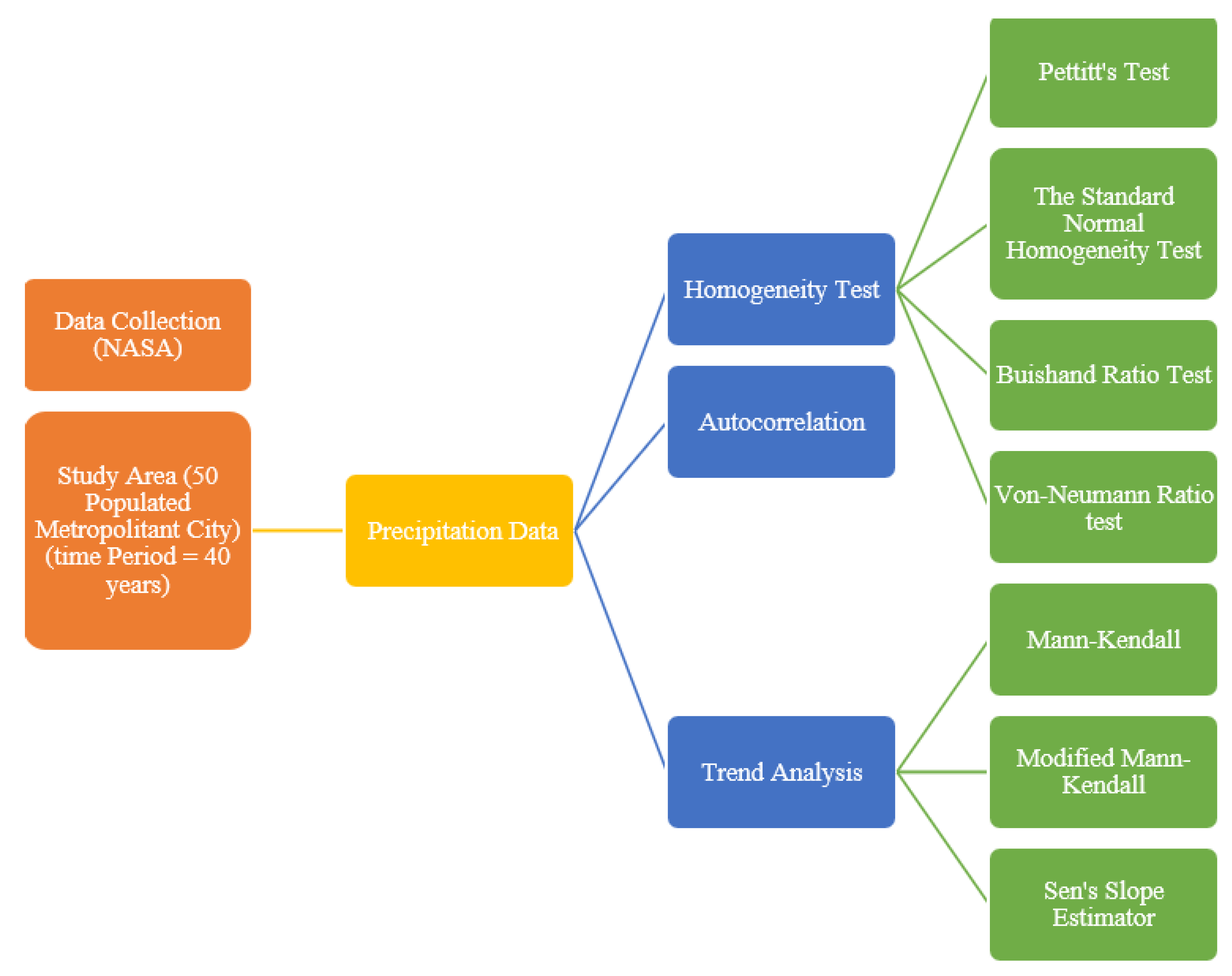
2. Materials and Methods

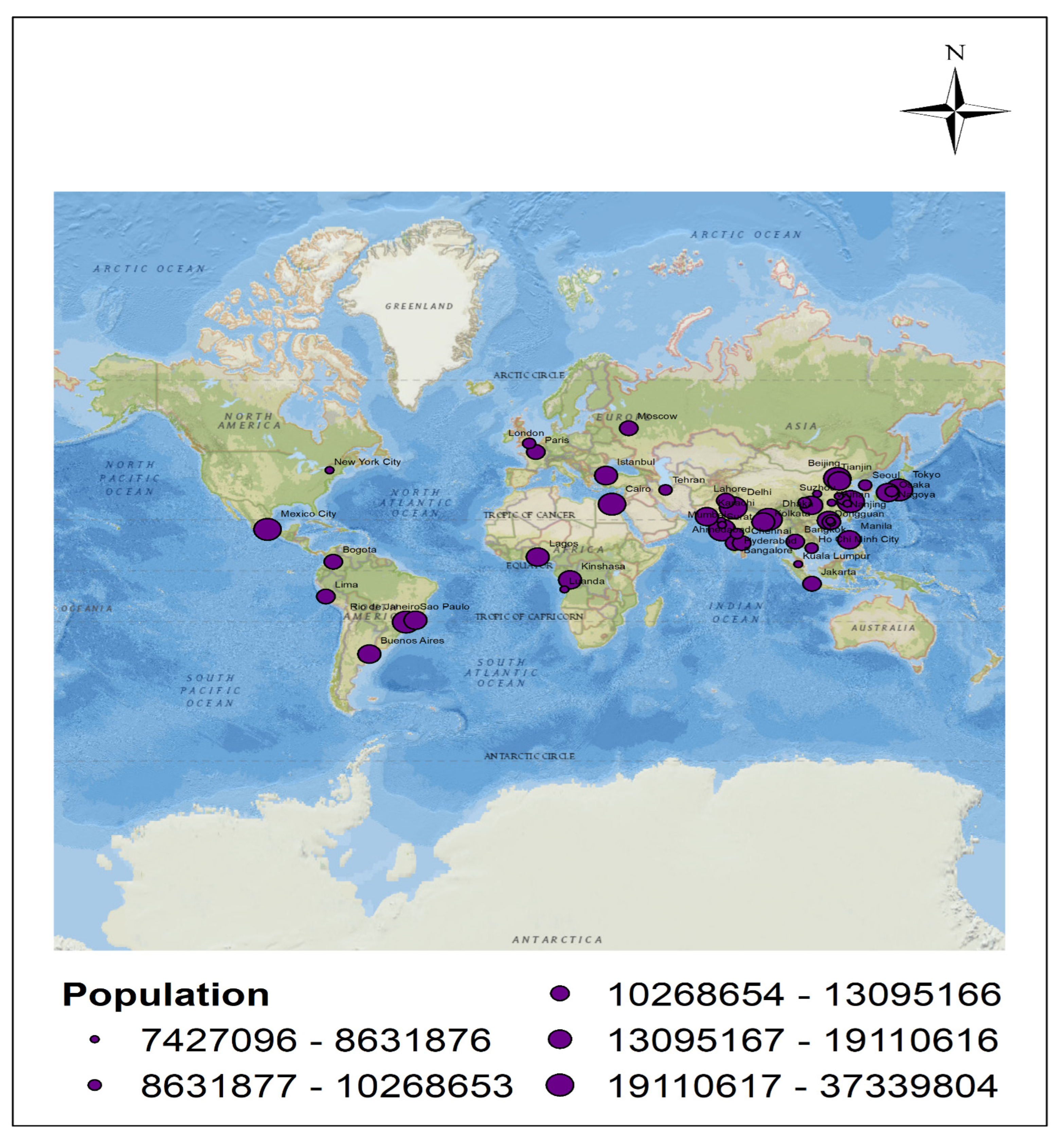
2.1. Study Area

To research climatic variables and statistical change in meteorological precipitation trend detection, the most densely inhabited metropolitan cities were chosen. It is critical to conduct a climatic change analysis because of the large population, urbanization, and extensive industrialization that are all dependent on numerous factors for the country’s and world’s progress. In 2050, the world’s population is expected to reach 9.6 billion, with 66% of the people living in cities [33]. The 50 cities in this study were chosen from 26 different countries throughout the world (Figure 1). Only eight cities were chosen in India: Delhi, Mumbai, Kolkata, Bangalore, Chennai, Hyderabad, Ahmedabad, and Surat, where Delhi is India’s capital. Most of the highly populated metropolitan city were located in Asia. All the city data are shown in

Table 1. Rank of cities showing increasing and decreasing population growth rate concerning different latitude and longitude between city centers of different countries.

City Rank	Lat. (°N)	Long. (°E)	City Name	Country Name	Population (2021)	Population (2020)	Growth Rate in %
1	35.6895	139.6916	Tokyo	Japan	37,339,804	37,393,128	−0.140
2	28.6423	77.1149	Delhi	India	31,181,376	30,290,936	2.940
3	31.2241	121.4574	Shanghai	China	27,795,702	27,058,480	2.720
4	−23.5613	−46.6547	Sao Paulo	Brazil	22,237,472	22,043,028	0.880
5	19.2803	−99.1408	Mexico City	Mexico	21,918,936	21,782,378	0.630
6	23.7139	90.3989	Dhaka	Bangladesh	21,741,090	21,005,860	3.500
7	30.0452	31.2353	Cairo	Egypt	21,322,750	20,900,604	2.020
8	39.9112	116.3917	Beijing	China	20,896,820	20,462,610	2.120
9	18.9409	72.8348	Mumbai	India	20,667,656	20,411,274	1.260
10	34.6947	135.5018	Osaka	Japan	19,110,616	19,165,340	−0.290
11	24.9061	67.0815	Karachi	Pakistan	16,459,472	16,093,786	2.270
12	29.5628	106.5528	Chongqing	China	16,382,376	15,872,179	3.210
13	41.0145	28.95	Istanbul	Turkey	15,415,197	15,190,336	1.480
14	−36.6668	−60.5776	Buenos Aires	Argentina	15,257,673	15,153,729	0.690
15	22.5713	88.3706	Kolkata	India	14,974,073	14,850,066	0.840
16	−4.3218	15.3081	Kinshasa	DR Congo	14,970,460	14,342,439	4.380
17	6.4866	3.1583	Lagos	Nigeria	14,862,111	14,368,332	3.440
18	14.6006	120.985	Manila	Philippines	14,158,573	13,923,452	1.690
19	39.1445	117.1767	Tianjin	China	13,794,450	13,589,078	1.510
20	23.1163	113.2494	Guangzhou	China	13,635,397	13,301,532	2.510
21	−22.8258	−43.1963	Rio de Janeiro	Brazil	13,544,462	13,458,075	0.640
22	31.5404	74.3028	Lahore	Pakistan	13,095,166	12,642,423	3.580
23	12.9683	77.5862	Bangalore	India	12,764,935	12,326,532	3.560
24	55.7649	37.6095	Moscow	Russia	12,593,252	12,537,954	0.440
25	22.5568	114.1189	Shenzhen	China	12,591,696	12,356,820	1.900
26	13.0843	80.2818	Chennai	India	11,235,018	10,971,108	2.410
27	4.3335	−74.2027	Bogota	Colombia	11,167,392	10,978,360	1.720
28	48.8536	2.349	Paris	France	11,078,546	11,017,230	0.560
29	−6.1715	106.8258	Jakarta	Indonesia	10,915,364	10,770,487	1.350
30	−12.0556	−77.0268	Lima	Peru	10,882,757	10,719,188	1.530
31	13.7557	100.5002	Bangkok	Thailand	10,722,815	10,539,415	1.740
32	17.3959	78.4708	Hyderabad	India	10,268,653	10,004,144	2.640
33	37.5695	126.9751	Seoul	South Korea	9,967,677	9,963,452	0.040
34	35.1917	136.9053	Nagoya	Japan	9,565,642	9,552,132	0.140
35	51.5092	−0.1277	London	United Kingdom	9,425,622	9,304,016	1.310
36	30.6724	104.0753	Chengdu	China	9,305,116	9,135,768	1.850
37	35.6897	51.415	Tehran	Iran	9,259,009	9,134,708	1.360
38	32.0502	118.7658	Nanjing	China	9,143,980	8,847,372	3.350
39	10.7481	106.7	Ho Chi Minh City	Vietnam	8,837,544	8,602,317	2.730
40	−8.8147	13.2322	Luanda	Angola	8,631,876	8,329,798	3.630
41	30.6434	114.324	Wuhan	China	8,473,405	8,364,977	1.300
42	34.2501	108.867	Xi-an Shaanxi	China	8,274,651	8,000,965	3.420
43	23.0278	72.5992	Ahmedabad	India	8,253,226	8,059,441	2.400
44	42.9352	−75.6546	New York City	United States	8,230,290	8,283,550	−0.640
45	3.1482	101.6939	Kuala Lumpur	Malaysia	8,210,745	7,996,830	2.670
46	30.2724	120.2059	Hangzhou	China	7,845,501	7,642,147	2.660
47	22.2784	114.1604	Hong Kong	Hong Kong	7,598,189	7,547,652	0.670
48	21.1868	72.8367	Surat	India	7,489,742	7,184,590	4.250
49	23.0446	113.7369	Dongguan	China	7,451,889	7,407,852	0.590
50	33.3641	117.0036	Suzhou	China	7,427,096	7,069,992	5.050

.

The metropolitan areas of London and New York, with populations of 9,425,622 and 8,230,290, respectively, are growing and shrinking at rates of 1.307% and −0.643% of the developed countries of the United Kingdom and the United States. In this case, the maximum growth rate is dropping in New York. Suzhou has a population of 7,427,096 people and is growing at a pace of 5.051% in China. Buenos Aires is a city in Argentina with a population of 15,257,673 people and a growth rate of 0.686%. The majority of Mexico’s population is concentrated in the province of Mexico City.

2.2. Data Source

To detect the trend analysis of the precipitation assessment, changing rainfall precipitation data for the 50 major cities was acquired from the National Aeronautics and Space Administration (NASA) over 40 years (1981–2020) of different months (January to December). It provides critical data for studying climate and climate processes using high-powered satellite systems. These are climatologically averaged estimates of meteorological parameters and surface solar energy fluxes over a lengthy period.

Based on the well-known NASA Goddard’s Global Modeling and Assimilation Office (GMAO) assimilation model, theModern Era Retrospective-Analysis for Research and Applications (MERRA2) and the POWER meteorological precipitation parameters provided by the project and specified within this validation section are used to validate the data, with a spatial grid resolution of ½° × ⅝° [34,35].

2.3. Methods

The research methodology proposed in the present study is shown in detail in the following Figure 2.

2.3.1. Homogeneity Test

One of the most essential ways of evaluating the period where a major change in the time series happened is the homogeneity or change point detection test. The change point in the climatic series is detected using four methods: (i) Pettitt’s Test, (ii) Standard Normal Homogeneity Test, (iii) Buishand Range Test, and (iv) Van-Neumann Ratio Test. The application of several change point tests is described in detail below [36]:

Pettitt’s Test

Pettitt’s test is a non-parametric rank-based technique for determining the occurrence of a breakpoint (year or month) in a climatic records series [37]. This test is less sensitive than the others and sensitive for breaking a time series in the middle, according to its ranking. The following formula is used to calculate this test statistic:

$$Z_k=2{\displaystyle \sum }_{i=1}^k{R}_i-k\left(n+1\right) k=1,2,\dots , n$$

(1)

When a K-year break occurs, the statistic around the year k = K is maximum or minimum, and Z_K = max Z_k occurs when the break occurs.

Standard Normal Homogeneity Test (SNHT)

The static$T_k$ value with n data points is used to compare the first mean (n) observations and the remaining mean (n − k) observations [38]:

$$T_k=k{Z}_1^2+\left(n-k\right)Z_2^2 k=1,2,\dots \dots \dots n$$

(2)

Z₁ and Z₂ are calculated using the equations:

$$Z_1=\frac{1}{k}{\displaystyle \sum }_{i=1}^k\frac{\left(x_i-\overline{x}\right)}{\sigma x}$$

(3)

$$Z_2=\frac{1}{n-k}{\displaystyle \sum }_{i=k+1}^n\frac{\left(x_i-\overline{x}\right)}{\sigma x}$$

(4)

where $\overline{x}$ is the series’ mean value and $\sigma x$ is the series’ standard deviation, and, $T_k$ is the series’ maximum value, with year k as the changing point. The null hypothesis is rejected when the test statistic is greater than the critical value, depending on the size of the sample n.

The Buishand Range Test

Buishand [39] originally proposed this parametric test. In more detail, S_k stands for adjusted partial sums, which is a cumulative deviation from the mean to the k^th set of observations:

$$S_k={\displaystyle \sum }_{i=1}^k \left(x_i-\overline{x}\right) k=1,2,\dots ,n$$

(5)

where $\overline{x}$ is mean time series observations (x₁, x₂, x₃, …, x_n) and k is the observation number when the breakpoint is occurring.

$$\mathit{R}=\frac{\mathit{M}\mathit{a}\mathit{x}\left({\mathit{S}}_{\mathit{k}}\right)-\mathit{M}\mathit{i}\mathit{n}\left({\mathit{S}}_{\mathit{k}}\right)}{\overline{\mathit{x}}}$$

(6)

The $R/\sqrt{n}$ value is calculated and compared to the critical values.

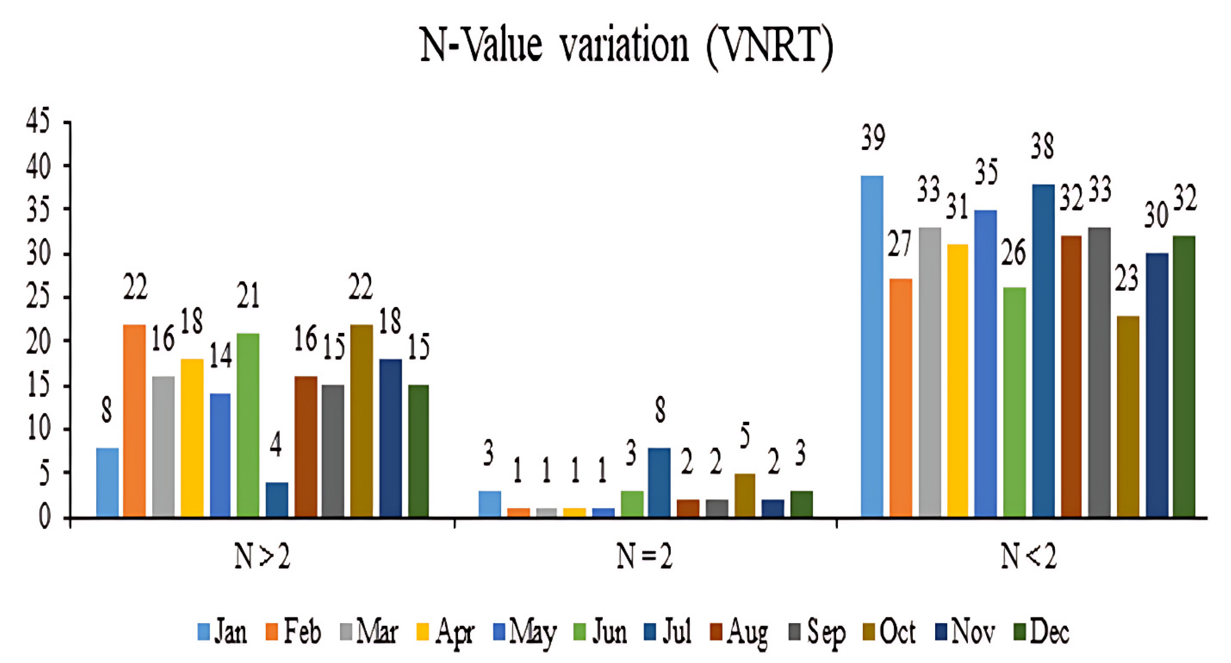
The Van-Neumann Ratio Test

The Van-Neumann Ratio is a widely used test that measures the difference between mean square consecutive (year to year) and variance. The break year is not reflected by this parametric test. Because of its sensitivity to deviations from homogeneity, this test ratio is more complimentary than other tests. The change point detection using this statistical test can be expressed as x₁, x₂, x₃, …, x_n observations in a time series.

$$N=\frac{{{\displaystyle \sum }}_{i=1}^{n-1}{\left(x_i-x_{i-1}\right)}^2}{{{\displaystyle \sum }}_{i=1}^n{\left(x_i-\overline{x}\right)}^2}$$

(7)

When N = 2 is the predicted value, the sample is homogeneous. Inhomogeneity or a sample break is indicated by a low value of N (less than 2).

2.3.2. Trend Analysis

Auto Correlation Factor

The primary issues in defining the trend in time series data using autocorrelation are determined. The variance dependency of the Mann–Kendall (MK) test on the degree of serialism. When the time series does not have a realistic trend, a substantial trend is detected, and positive serial dependence for the time series data increases the type I error. For all data series, the autocorrelation factor was calculated at a significant level of 0.5 [40,41].

$$r_k=\frac{{{\displaystyle \sum }}_{k=1}^{N-K}\left(y_t-y_t\right)\left(y_{t+k}-y_{t+k}\right)}{\left[{{\displaystyle \sum }}_{k=1}^{n=k},{\left(y_t-y_t\right)}^2,{\left(y_{t+k}-y_{t+k}\right)}^2\right]{}^{0.5}}$$

(8)

Here, $r_k$ is the autocorrelation function for observed data flow time series, y_t and y is the average time series at lag k, and N is the total length of time series y_t and maximum lag k.

The Mann–Kendall (MK) Test

The Mann–Kendall Test is a non-parametric test that is commonly used for trend analysis in climatologic and water hydrologic time series.

Random and low sensitivity to abrupt breaks for inhomogeneous time series is used in this test dataset.

The Mann–Kendall Test S statistic is followed by

$$S={\displaystyle \sum }_{i=1}^{n-1}{\displaystyle \sum }_{j=i+1}^{n}sign \left(X_j-X_i\right)$$

(9)

Here, X_j and X_i are annual data values in year j and i, respectively, when i = 1, 2, 3, 4, …, n − 1 and j = 1, 2, 3, 4, …, n.

$$sign\left(X_j-X_k\right)=\left\{\begin{array}{c}+1 if X_j-X_k>0\\ 0 if X_j-X_k=0\\ -1 if X_j-X_k<0\end{array}\right.$$

(10)

When the positive value of a statistic (S) is very high, the trend increases, and when the negative value of the statistic (S) is very low, the trend drops (S). For scientifically quantifying the trend significance, it is defined as the probability linked with statistic S and sample size n. When the sample size is big (n > 10), the variance statistic is calculated using normal approximation and mean value as follows:

$$Variance ({\sigma }^2)=\frac{n\left(n-1\right)\left(2n+5\right)-{{\displaystyle \sum }}_{i=1}^m{t}_i\left(t_i-1\right)\left(2t_i+5\right)}{18}$$

(11)

In this equation, the number of data points is n, the number of tied groups is m (tied groups are groupings of sample data with the same value), and the number of data points in the group i^th is $t_i$. Z_s is a standard test statistic that is defined as follows:

$$Z_s=\left\{\begin{array}{c}\frac{S-1}{\sigma } for S>0\\ 0 for s=0\\ \frac{S+1}{\sigma } for S<0\end{array}\right.$$

(12)

|Z_s| exceeds Z_α/2, where α = 0.05 denotes the two-sided test’s specified local significance level (5% with Z_0.025 = 1.96). At this significant level, values of more than 1.96 and less than 1.96, respectively, show a highly (p < 0.05) positive (growing) and negative (decreasing) trend. Otherwise |Z_s| is smaller than Z_α/2, the null hypothesis is accepted, and the time series shows no trend [42].

The Modified Mann–Kendall Test

To observe the trend detection with an autocorrelation series, the Modified Mann–Kendall (MMK) was used [43]. In this study, the autocorrelation between ranks of the observations ρ_k has been estimated after subtracting an estimate of the non-parametric trend such as Sen’s median slope of the data.

For the variance correction factor $n$/$n_s^{*}$ calculated by using statistically significant ρ_k values, the variance of S is underestimated for the positively auto correlated data:

$$\frac{n}{n_s^{*}}=1+\frac{2}{n\left(n-1\right)\left(n-2\right)}\times {\displaystyle \sum }_{k=1}^{n-1}\left(n-k\right)\left(n-k-1\right)\left(n-k-2\right){\rho }_k$$

(13)

where n is the actual number of observations, $n_s^{*}$ is an effective number of observations to account for data autocorrelation, and ${\rho }_k$ is the autocorrelation function for the rank of the observations. Here is the corrected variance:

$$V^{*}\left(S\right)=V\left({\sigma }^2\right)\times \frac{n}{n_s^{*}}$$

(14)

where $V\left({\sigma }^2\right)$ is a variance calculated from the MK Test.

Sen’s Slope Estimator Test

The non-parametric Sen’s slope statistics are proposed by Sen [44]. The magnitude (slope) of the trend in a sample of n pairs of data is estimated using this method. All data pairs’ slopes can be determined as follows:

$$Q_i=\frac{\left(X_j-X_k\right)}{j-k} where \left(j>k\right)\left(for i = 1,2,3,\dots ,n\right)$$

(15)

where $X_j$ and $X_k$ represent the data values at time $j$ and $k$ (j > k), respectively. When considering

$$Q_{med}=\left\{\begin{array}{c}Q\left[\frac{n+1}{2}\right] if n is odd\\ \frac{Q_{n/2}+Q_{\left(n+2\right)/2}}{2} if n is even\end{array}\right.$$

(16)

where $Q_{med}$ represents the data trend, a positive $Q_{med}$ value indicates an upward trend and a negative $Q_{med}$ value indicates a downward nature of the trend in the time series.

3. Results

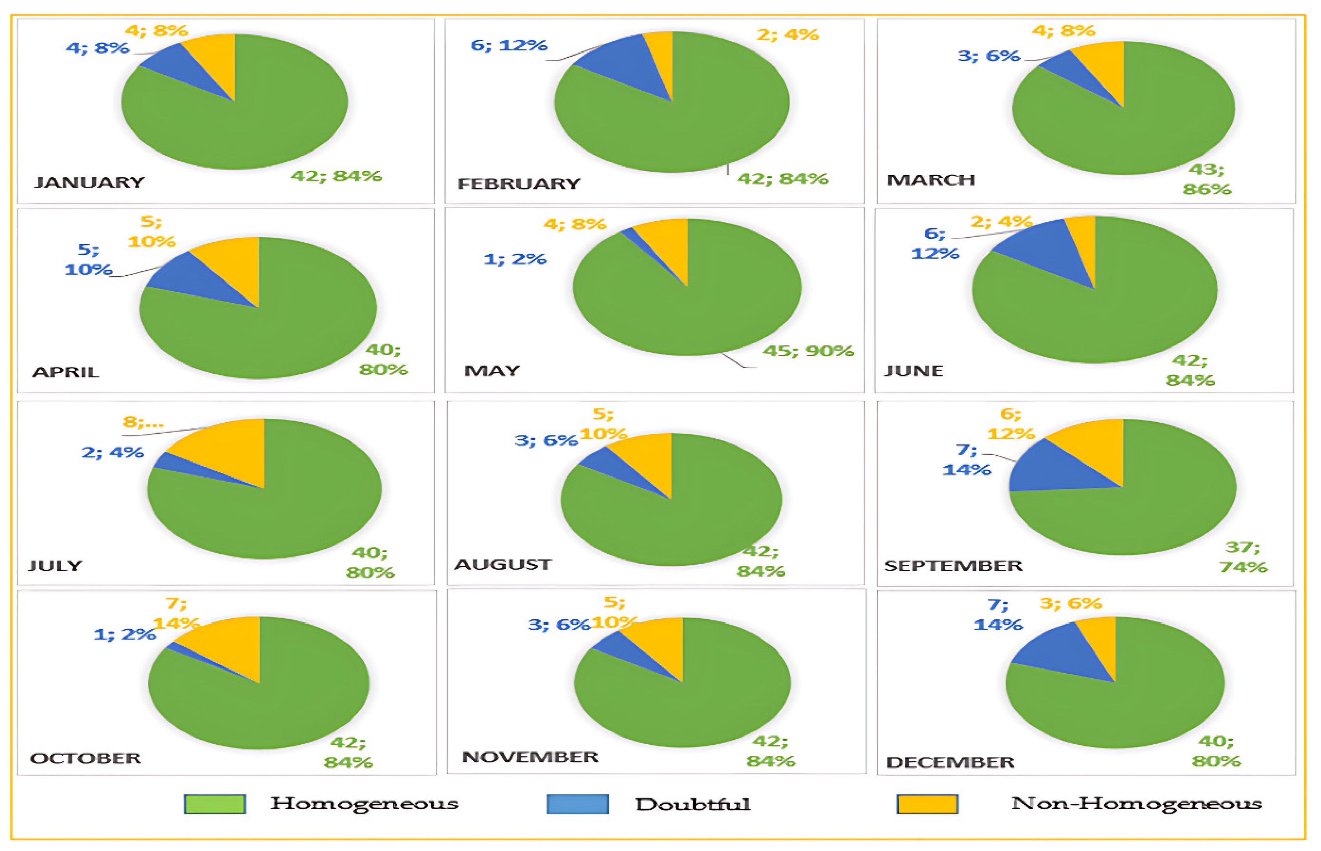
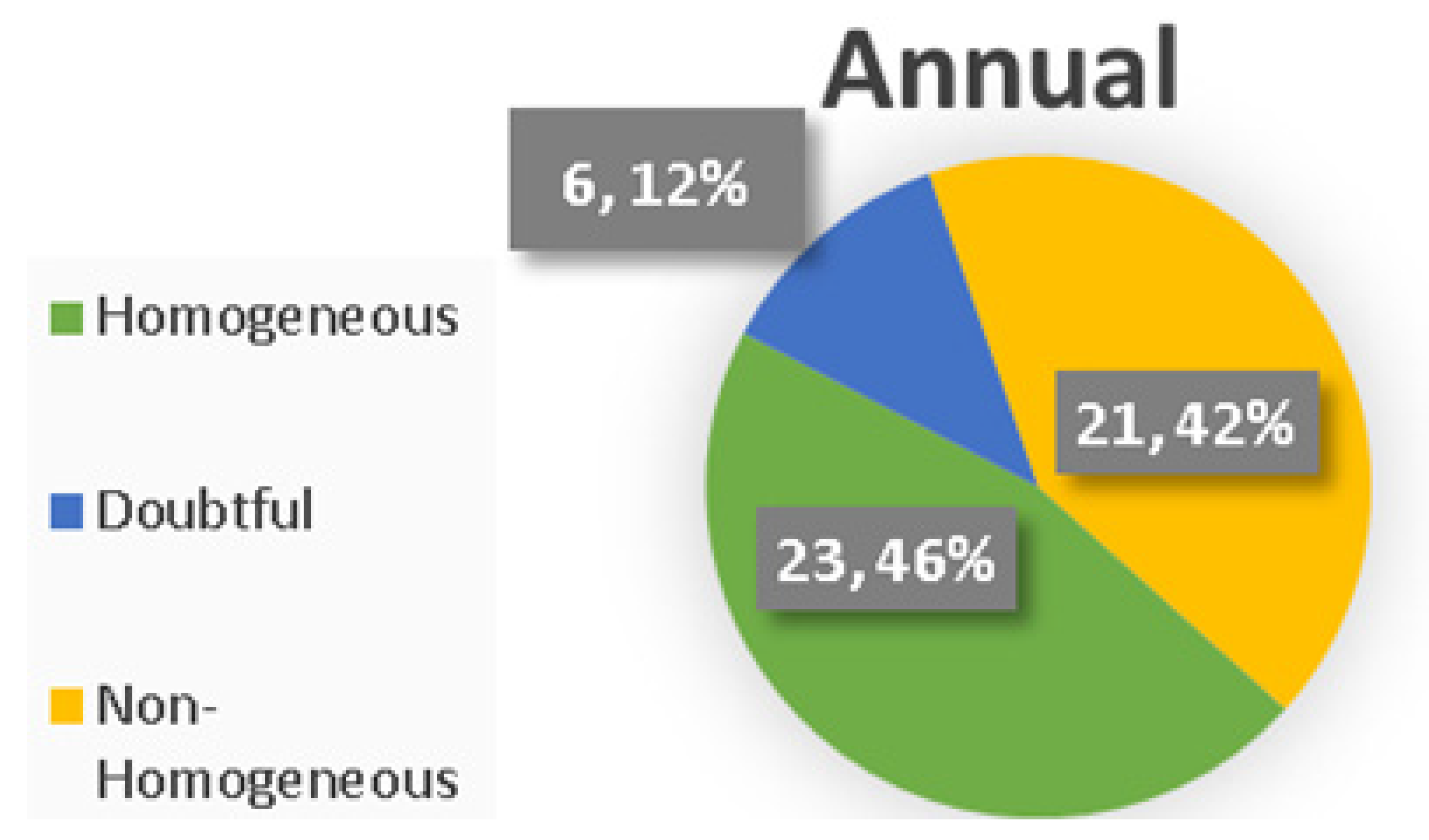
3.1. Homogeneity Test Result

3.1.1. Monthly Homogeneity Test

In January, 42 (84%) cities were homogenous, and as shown in Figure 3 and Figure 4 (8%) were doubtful, such as Shanghai, Sao Paulo, Lahore, and Wuhan, and 4 (8%) were non-homogeneous, such as Istanbul, Manila, Bogota, and Kuala Lumpur. The observed value of N > 2 in the VNRT for January month had 8 cities. Rio de Janeiro (2.453) had the greatest score, whereas Hong Kong (2.056) had the lowest. In these cities, rapid variations are present. N = 2 was found in only three cities (Delhi, Tehran, and Nanjing), and the series is considered homogeneous. The remaining 39 cities became < 2, indicating cities with changing points, as shown in Figure 5. The figures range from 1.968 (Chengdu) to 0.772 (Beijing) (Mumbai). The majority of the breakpoint was detected in 1988 (11 cities), according to Pettitt’s tests (Dongguan, Guangzhou, Hangzhou, Hong Kong, Nagoya, Nanjing, Osaka, Paris, Shenzhen, Tokyo, and Wuhan).

In February, 42 (84%) cities were homogenous, 6 (12%) cities were doubtful (Karachi, Manila, Rio de Janeiro, Lima, Tehran, and Luanda), and 2 (4%) cities were non-homogeneous (Bogota and Jakarta), as shown in Figure 3. The observed value of N > 2 in the VNRT for February month had 22 cities. Lahore (2.612) was the highest, whereas Ho Chi Minh City (2.052) was the lowest. In these cities, there were frequent changes. Only Moscow city was found with N = 2; thus, the series is considered homogeneous. The remaining 27 cities become < 2, indicating that these are the cities with changing points, as shown in Figure 5. The figure varies from 1.926 (Seoul) to 0.821 (Tokyo) (Jakarta). According to Pettitt’s testing, most of the breakpoint appeared in 1998 (8 cities) (Bangalore, Chengdu, Dongguan, Guangzhou, Hong Kong, Kolkata, Manila, Shenzhen).

In March, 43 (86%) cities were homogeneous, whereas 3 (6%), including Sao Paulo, Mumbai, and Chongqing, and 4 (8%), including Manila, Jakarta, Chengdu, and Luanda, were doubtful and non-homogeneous, as shown in Figure 3. The observed value of N > 2 had 16 cities in the VNRT for March. The highest was Osaka (2.562), whereas the lowest was Karachi (2.041). In these cities, where there were frequent changes. Only Chennai city has N = 2, hence the series is considered homogeneous. The remaining 33 cities were N < 2, indicating that these were the cities with changing points, as shown in Figure 5. The figures range from 1.977 (Bangalore) to 1.225 (Hyderabad) (Manila). Most of the breakpoint was observed in 2003 (5 cities), according to Pettitt’s tests (Buenos Aires, Chengdu, Chongqing, Jakarta, Shanghai).

In April, 40 (80%) cities were homogeneous, as shown in Figure 3, the doubtful 5 (10%) cities were Delhi, Dhaka, Shenzhen, Hong Kong, Suzhou, and the non-homogeneous 5 (10%) cities were Sao Paulo, Cairo, Chongqing, Rio de Janeiro, and Tehran. In the VNRT for April, the observed value of N > 2 had 18 cities. Among them, New York (2.525) was the highest and Suzhou (2.063) was the lowest. In these cities, rapid variations were present. N = 2 was also found in only Lima city, and so the series is considered homogenous. The rest of the 31 cities became < 2, which means that these cities had change points, which are shown in Figure 5. The number ranges from 1.922 (Shenzhen and Hong Kong) to 1.182 (Rio de Janeiro). According to Pettitt’s tests, most of the breakpoint was discovered in 2001 (11 cities) (Dongguan, Guangzhou, Hong Kong, London, Nanjing, New York City, Paris, Seoul, Shanghai, Shenzhen, and Tehran).

In May, 45 (90%) cities were homogenous, with the highest number of homogeneous cities compared to other months, whereas 1 (2%) city, Sao Paulo, was questionable, and 4 (8%) cities, such as Dhaka, Karachi, Manila, and Ho Chi Min City, were non-homogeneous, as shown in Figure 3. The observed value of N > 2 has 14 cities in the VNRT for May. Shanghai (2.635) has the greatest score, and New York (2.199) has the lowest. In these cities, there were frequent changes. Only Bangalore city has N = 2, hence the series is considered homogeneous. The remaining 35 cities had N < 2, indicating that these were the cities with changing points, as shown in Figure 5. The figures range from 1.985 (Moscow) to 0.680 (Berlin) (Karachi). Most of the breakpoint was detected in 2011 (6 cities), according to Pettitt’s tests (Hangzhou, Istanbul, Nagoya, Osaka, Seoul, and Shanghai).

In June, 42 (84%) cities were homogenous, 6 (12%) cities were doubtful, including Chongqing, Lahore, Hyderabad, Ho Chi Min City, Kuala Lumpur, and Surat, and 2 (4%) cities such as Dhaka and Tehran were non-homogeneous, as shown in Figure 3. The observed value of N > 2 in the VNRT for June month had 21 cities. The highest was Mumbai (2.642) and the lowest was Beijing (2.049). In these cities, where there are frequent changes. The series is homogeneous since it includes Rio de Janeiro, Jakarta, and Suzhou, with N = 2. The remaining 26 cities become < 2, indicating that these are the cities with changing points, as shown in Figure 7. The figure varies from 1.971 (Seoul) to 0.862 (Tokyo) (Ho Chi Min City). According to Pettitt’s tests, the majority of the breakpoint was discovered in 2000 (5 cities) (Beijing, Dhaka, Mumbai, Surat, and Tianjin) and 2014 (5 cities) (Kuala Lumpur, Nanjing, Suzhou, Wuhan, and Xi-an Shaanxi).

For July, 40 (80%) cities were homogenous, 2 (4%), such as Kuala Lumpur and Rio de Janeiro, were dubious, and 8 (16%) cities, such as Dhaka, Mumbai, Lagos, Shenzhen, Lima, Tehran, Ho Chi Min City, and Hong Kong, were non-homogeneous, as represented in Figure 3. The observed value of N > 2 in the VNRT for July month had four cities, as shown in Figure 5. The highest was in Delhi (2.563), and the lowest was in Buenos Aires (2.104). In these cities, there were frequent changes. The series is homogeneous since it includes Moscow, Bangkok, London, Nanjing, Xi-an Shaanxi, Ahmedabad, Hangzhou, and New York, where N = 2. The remaining 38 cities are N < 2, indicating that these are the cities with changing points. The figures range from 1.981 (Kinshasa) to 0.914 (Dhaka). According to Pettitt’s tests, the majority of the breakpoint was discovered in 2002 (9 cities) (Bangkok, Delhi, Dongguan, Guangzhou, Hong Kong, New York City, Shenzhen, Surat, and Xi-an Shaanxi).

In August 42 (%) cities were homogeneous, as shown in Figure 3, 3 (6%) cities such as Karachi, Tehran, and Ahmedabad were doubtful, and 5 (10%) cities were non-homogeneous such as Dhaka, Manila, Ho Chi Min City, Surat, and Suzhou. In the VNRT for August, the observed value of N > 2 had 16 cities, as shown in Figure 5. Among them, Jakarta (2.766) is the highest, and Bangalore (2.055) is the lowest. In these cities, rapid variations are present. In Mumbai and Nagoya, where N = 2, the series is deemed homogeneous. The rest of the 32 cities became < 2 which means these cities were the ones where change points were present. The number ranges from 1.979 (Lima) to 0.821 (Karachi). According to Pettitt’s tests, the majority of the breakpoint was discovered in 2002 (8 cities) (Ahmedabad, Hong Kong, Mexico City, New York City, Sao Paulo, Shenzhen, Suzhou, and Xi-an Shaanxi).

September month’s homogeneous cities’ numbers are 37 (74%), doubtful and non-homogeneous are 7 (14%), such as in Dhaka, Lagos, Tianjin, Lima, Hyderabad, Ahmedabad, and Hangzhou, and 6 (12%) in Shanghai, Chongqing, Manila, Bogota, Tehran, and Surat, as shown in Figure 3. In the VNRT for September, the observed value of N > 2 had 15 cities, as shown in Figure 5. Among them, Bangalore (2.529) was the highest and Nagoya (2.050) was the lowest. In these cities, rapid variations were present. In Buenos Aires and Kinshasa, where N = 2, the series was deemed homogeneous. The rest of the 33 cities became < 2, which means these cities were the ones where change points were present. The number ranges from 1.974 (Seoul) to 0.930 (Bogota). According to Pettitt’s tests, the majority of the breakpoint was discovered in 2003 (8 cities) (Chennai, Dhaka, Dongguan, Hong Kong, Karachi, Rio de Janeiro, Shenzhen, and Suzhou).

For October, 42 (84%) cities were homogenous, only one (2%) city, Beijing, was questionable, and seven (14%), including Dhaka, Chongqing, Bogota, Chengdu, Tehran, Ho Chi Min City, and New York, were non-homogeneous, as shown in Figure 3. The observed value of N > 2 had 22 cities in the VNRT for October. Bangalore had the highest score (2.515) and Bangkok had the lowest score (2.046). In these cities, there were frequent changes. The series was homogeneous since it includes Kolkata, Lagos, Lahore, Surat, and Wuhan, where N = 2, as shown in Figure 5. The remaining 23 cities became <2, indicating that these are the cities with changing points. The figures range from 1.920 (Mumbai) to 1.263 (Bangalore) (Chengdu). According Pettitt’s tests, the majority of the breakpoint was discovered in 1997 (5 cities) (Dhaka, Kolkata, Manila, Nagoya, and Osaka).

In November, 42 (84%) cities were homogeneous, with 3 (6%) cities such as Delhi, Cairo, and Lahore and 5 (10%) cities such as Lagos, Rio de Janeiro, Tehran, Ho Chi Min City, and Xi-an Shaanxi were all doubtful and non-homogeneous, as shown in Figure 3. The observed value of N > 2 in the VNRT for November had 18 cities, as shown in Figure 5. Kuala Lumpur (2.731) had the greatest score and Istanbul (2.136) had the lowest. In these cities, there were frequent changes. The series wass considered homogeneous because it includes Moscow and Hyderabad, where N = 2. The remaining 30 cities are reduced to two, indicating the cities with changing points. The number ranges from 1.947 (Nanjing) to 0.724 (Lagos). The majority of the breakpoint was detected in 1998, according to Pettitt’s tests (8 cities) (Chengdu, Chongqing, Hyderabad, Kuala Lumpur, Manila, Seoul, Surat, and Tokyo).

In the last month, December, numbers of the city for homogeneous were 40 (80%), as shown in Figure 3, doubtful and non-homogeneous were 7 (14%) cities, such as Tokyo, Osaka, Karachi, Rio de Janeiro, Moscow, Ho Chi Min City, Surat, and 3 (6%) cities such as Manila, Nagoya, and Tehran, respectively. In the VNRT December month, the observed value of N > 2 had 15 cities, as shown in Figure 5. Among them, Lagos (2.374) was the highest, and Cairo (2.049) was the lowest. In these cities, rapid variations were present. In Osaka, Buenos Aires, and Dongguan, where N = 2, the series was deemed homogeneous. The rest of the 32 cities became < 2, which means these cities were the ones where change points are present. The number ranges from 1.986 (Shenzhen and Hong Kong) to 0.984 (Karachi). The majority of the breakpoint was detected in 2001 (6 cities), according to Pettitt’s tests (Chengdu, Istanbul, Karachi, Nagoya, New York City, and Osaka).

3.1.2. Annual Homogeneity Test

By analyzing four tests (Pettitt’s, SNHT, Buishand, and Von Neumann Test) using annual precipitation data, six cities were classified as doubtful, including Rio de Janeiro, Bogota, Paris, Jakarta, Nagoya, and Ahmedabad. The remaining 23 cities were homogeneous, whereas the remaining 21 cities were non-homogeneous, as shown in Figure 4. The observed value of N > 2 in the VNRT had four cities with rapid fluctuations, including Mexico City (2.052), Kolkata (2.202), and Delhi (2.282). In Guangzhou and Chennai, where N = 2, the series was deemed homogeneous. The rest of the 45 cities became < 2, which means these cities were the ones where change points were present. The number ranges from 0.607 (Dhaka) to 1.893 (Tianjin). According Pettitt’s tests, most of the breakpoint was discovered in 1997 (Bangkok, Dhaka, London, Manila, Nagoya, Osaka, and Tokyo).

3.2. Trend Test Result

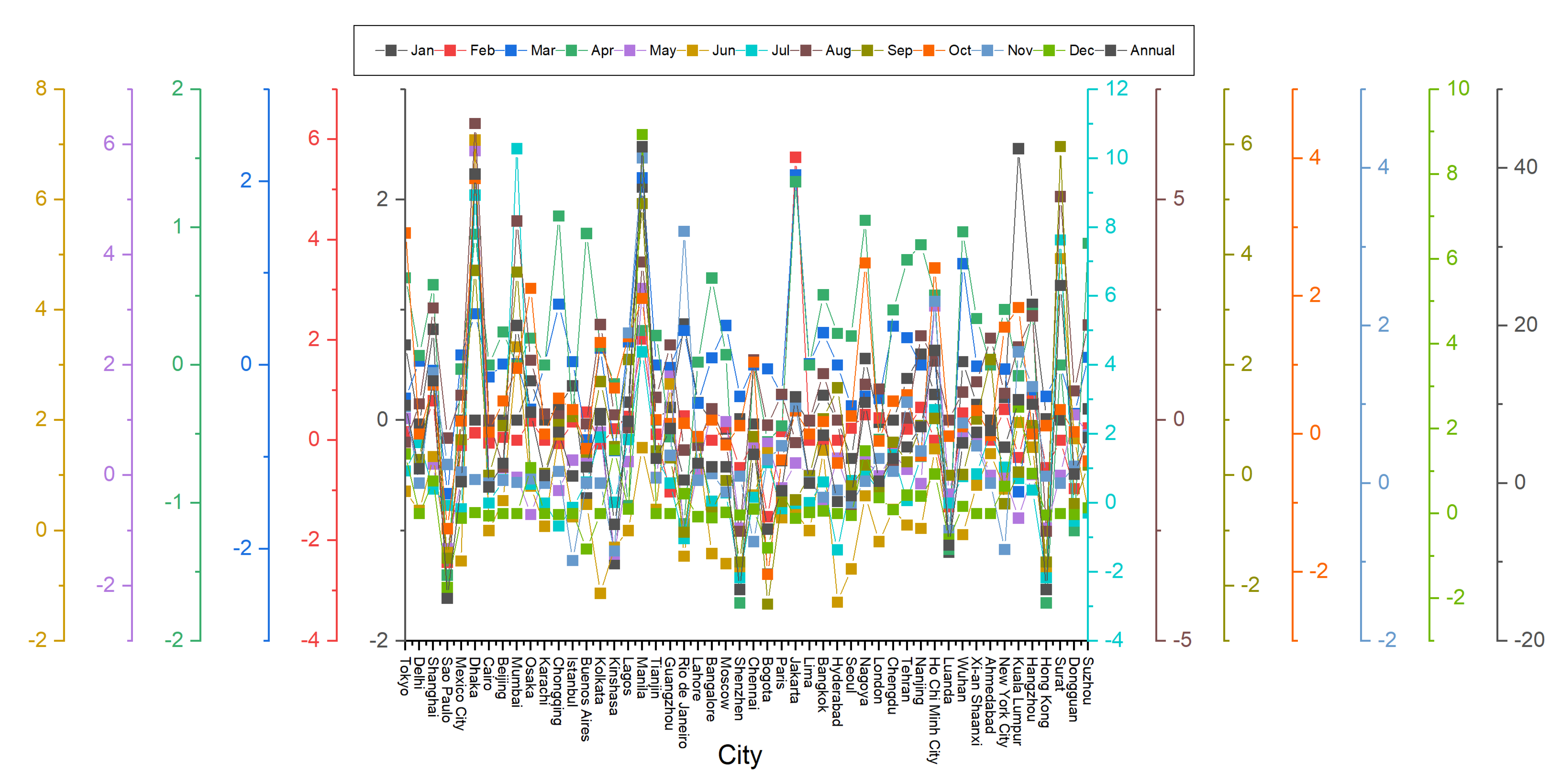
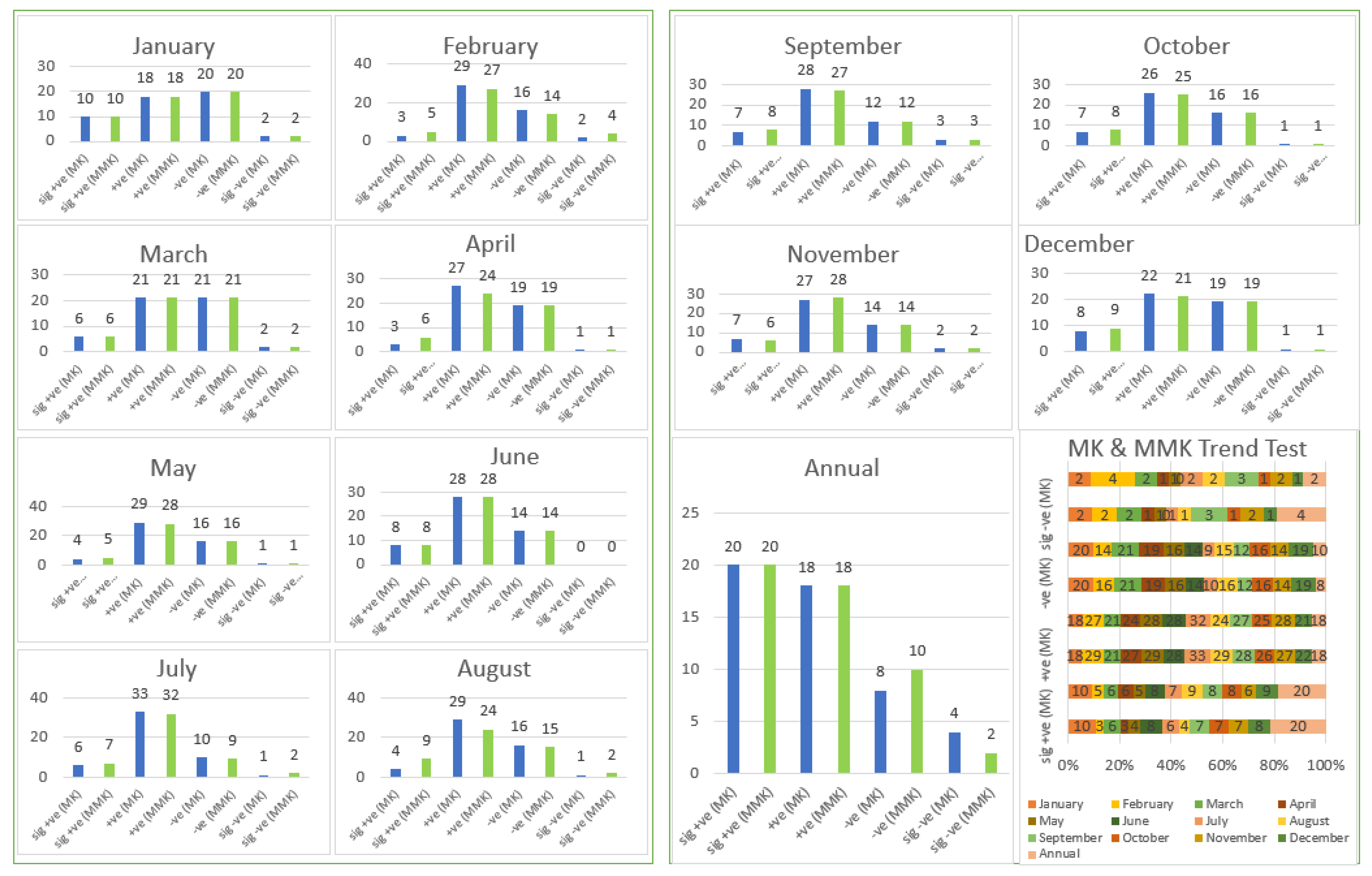
3.2.1. Monthly Mann–Kendall (MK) and Modified Mann–Kendall (MMK)

The Modified Mann–Kendall and Sen’s slope estimator tests were performed to define the trend and magnitude of the precipitation both monthly and annually over selected cities. The Modified Mann–Kendall test method has test results that are more accurate than the Mann–Kendall test. The non-parametric MMK test results analyzed the monthly precipitation to change the trend and magnitude of the 50 cities in different months from 1981 to 2020. Sen’s slope determined the precipitation data as 26% (13 cities) negative and 74% (37 cities) positive magnitude, as shown in Figure 6.

In January, the Z statistics of precipitation data from Mann–Kendall for the 50 most populated metropolitan cities are displayed in Figure 7. According to a 95% significance threshold, the Z statistics are divided into four categories: Z > 1.96 as a significant positive trend, Z in between 1.96 and 0 as a positive trend, Z in between 0 and −1.96 as a negative trend, and Z < −1.96 as a significant negative trend. The data ranges from −3.1464 (Luanda) to 2.7036 (Shanghai). Figure 7 shows the variation of Z statistics data from the Modified Mann–Kendall test, which varies from −3.1464 (Luanda) to 3.0105 (Saudi Arabia) (Manila) shown in

Table 2. Monthly and annual Z Statistics Value.

City Rank	Name	Country	Jan	Feb	Mar	Apr	May	Jun	Jul	Aug	Sep	Oct	Nov	Dec	Annual
1	Tokyo	Japan	1.45	0.48	−0.63	1.00	1.06	1.04	0.99	−1.61	0.31	2.50	0.83	2.53	2.85
2	Delhi	India	−0.29	−0.17	0.71	0.41	0.99	0.22	1.30	0.69	0.22	−0.23	0.58	−0.11	1.65
3	Shanghai	China	2.70	1.63	−0.10	0.68	0.39	1.63	1.24	2.04	1.34	0.94	2.27	3.31	3.46
4	Sao Paulo	Brazil	−1.65	−1.77	−1.95	−2.10	−4.75	−0.51	−0.25	−0.83	−14.81	−1.92	0.16	−1.95	−3.40
5	Mexico City	Mexico	0.02	−1.49	1.18	−0.21	−0.33	−1.12	−0.45	0.90	1.58	0.07	0.68	−1.89	−0.23
6	Dhaka	Bangladesh	−0.11	0.76	1.36	0.92	3.47	3.81	3.62	4.59	3.11	3.27	0.70	0.27	3.26
7	Cairo	Egypt	−1.04	−0.97	−2.93	0.38	−0.72	0.05	0.30	−0.86	−0.18	1.08	0.09	−0.66	−0.43
8	Beijing	China	0.26	1.45	0.40	1.21	0.69	1.07	0.69	−0.93	3.06	2.57	0.52	−0.45	2.49
9	Mumbai	India	−0.01	0.79	2.05	−0.20	−0.41	1.18	2.27	1.48	1.11	0.92	0.08	0.22	2.57
10	Osaka	Japan	1.12	0.87	−0.90	0.30	−1.12	0.69	1.00	1.73	0.08	1.88	−0.08	2.18	2.24
11	Karachi	Pakistan	−0.53	−0.42	−0.24	−0.37	0.43	2.85	0.00	0.57	1.31	0.29	−0.09	0.45	0.76
12	Chongqing	China	1.49	−0.66	1.82	3.63	−0.56	2.28	−0.75	−0.23	1.17	1.57	0.68	−0.19	2.21
13	Istanbul	Turkey	0.30	0.92	0.00	−0.79	0.68	1.10	−0.91	0.76	3.01	0.84	−2.00	−0.60	0.17
14	Buenos Aires	Argentina	−1.63	0.57	−1.00	1.13	0.10	1.54	1.50	−0.14	1.08	−0.03	0.07	−1.32	0.69
15	Kolkata	India	−0.46	−0.71	0.70	0.16	0.70	−1.36	1.28	1.47	1.14	1.60	−0.20	0.46	2.40
16	Kinshasa	DR Congo	−1.01	0.28	−0.82	−0.07	−0.79	−1.18	0.74	1.49	1.47	0.57	−0.58	1.75	−1.17
17	Lagos	Nigeria	1.75	1.43	0.29	−1.47	0.24	−0.09	1.85	−0.46	1.93	2.06	5.16	1.10	1.84
18	Manila	Philippines	3.01	1.77	3.93	0.65	3.11	1.03	3.13	3.76	4.30	1.70	1.70	3.74	4.88
19	Tianjin	China	−0.25	3.45	−0.19	1.19	0.24	0.63	1.12	0.76	1.50	1.55	0.64	0.16	1.90
20	Guangzhou	China	0.33	−2.50	0.00	−0.79	1.33	1.88	0.05	2.03	0.41	0.00	0.40	−0.02	1.36
21	Rio de Janeiro	Brazil	0.55	0.58	0.62	−1.82	−1.21	−0.90	−2.69	−1.08	−1.43	0.40	3.22	0.33	0.45
22	Lahore	Pakistan	0.66	−0.86	−1.07	0.36	0.59	2.85	1.62	−0.33	1.40	−0.97	1.00	−0.71	0.71
23	Bangalore	India	−0.95	0.87	0.70	1.47	1.85	−1.24	0.29	0.39	−0.50	0.24	0.42	−0.51	0.57
24	Moscow	Russia	−0.58	1.27	3.40	0.40	3.19	−1.22	0.76	−1.03	−0.59	−0.73	−0.36	−0.15	0.57
25	Shenzhen	China	0.23	−0.89	−0.43	−1.43	−0.37	−0.19	−1.78	−1.06	−1.13	−0.05	−0.01	−0.28	−1.64
26	Chennai	India	−0.57	0.20	−0.04	0.52	3.88	1.56	0.24	1.80	0.69	0.23	0.08	0.23	0.96
27	Bogota	Colombia	−2.68	−3.09	−0.10	−0.97	0.16	2.35	2.78	−0.31	−2.06	−3.31	0.11	−1.31	−1.14
28	Paris	France	−1.32	0.81	−0.70	−1.77	−0.84	0.19	−0.68	1.34	−1.61	−0.77	1.12	0.92	−1.25
29	Jakarta	Indonesia	−0.07	3.78	2.61	2.30	1.09	0.22	−0.02	−3.14	−0.58	0.50	1.39	−0.30	1.39
30	Lima	Peru	−0.39	−0.19	0.23	−1.08	1.00	0.47	2.00	−0.81	−2.45	0.10	0.69	1.63	−0.33
31	Bangkok	Thailand	2.08	0.12	0.84	0.83	−0.80	2.49	1.01	1.46	2.74	0.54	−0.66	1.35	1.98
32	Hyderabad	India	−0.51	0.47	0.16	1.21	1.01	−1.47	−8.05	0.13	1.96	−0.51	−1.11	−1.15	−0.86
33	Seoul	South Korea	−1.62	1.28	−1.43	0.26	−0.55	−0.57	0.17	−0.92	0.00	0.52	−0.55	−0.24	−0.24
34	Nagoya	Japan	1.63	1.38	−0.97	1.06	0.16	0.78	0.94	0.44	0.24	2.27	−0.13	3.10	2.81
35	London	United Kingdom	0.06	1.64	−1.12	−1.29	−0.45	−0.23	0.71	3.22	−0.83	−0.23	0.69	1.08	0.70
36	Chengdu	China	0.34	−1.10	5.53	1.19	0.52	0.90	1.58	−2.40	1.00	2.76	0.91	1.26	1.67
37	Tehran	Iran	2.67	1.20	1.12	2.60	1.16	2.24	1.27	0.55	0.75	1.66	2.12	2.48	2.64
38	Nanjing	China	2.10	1.19	0.11	1.71	−0.48	0.24	1.22	1.88	1.33	−0.78	1.29	1.69	2.12
39	Ho Chi Minh City	Vietnam	2.37	1.53	2.32	1.41	1.45	1.48	2.45	0.91	1.35	2.06	4.62	3.34	1.69
40	Luanda	Angola	−3.15	−2.99	−3.43	−1.51	−0.85	−0.94	0.06	0.00	−0.34	−0.40	−1.35	−2.36	−3.03
41	Wuhan	China	2.14	1.44	1.34	2.01	2.11	0.22	1.20	0.66	0.22	0.11	1.82	0.97	1.33
42	Xi-an Shaanxi	China	2.24	1.96	−0.22	0.90	1.50	1.92	1.01	1.54	1.15	0.89	2.40	0.00	3.18
43	Ahmedabad	India	−1.22	0.10	0.05	−0.15	0.02	1.32	0.85	2.05	2.11	−0.71	−0.03	0.32	3.07
44	New York City	United States	0.78	3.04	0.19	1.28	0.08	1.19	2.03	1.78	−1.34	2.37	−1.97	1.83	7.14
45	Kuala Lumpur	Malaysia	2.35	−0.50	−1.49	−0.14	−0.74	1.88	1.18	1.61	0.00	1.74	1.48	2.41	3.19
46	Hangzhou	China	2.39	1.46	−0.36	0.27	0.05	1.62	0.99	2.24	0.75	−0.19	1.76	3.01	3.04
47	Hong Kong	Hong Kong	0.23	−0.89	−0.43	−1.43	−0.37	−0.19	−1.78	−1.06	−1.13	−0.05	−0.01	−0.28	−1.64
48	Surat	India	−0.68	−0.33	0.71	−0.58	0.19	1.97	1.62	2.23	3.59	0.79	−0.70	0.42	2.42
49	Dongguan	China	0.22	−2.21	−0.65	−1.42	0.79	1.22	−0.78	0.49	−0.29	−0.13	0.09	−0.31	0.03
50	Suzhou	China	0.91	1.35	0.30	2.86	1.19	0.43	0.02	2.53	0.03	−1.33	1.59	0.98	2.22
		>1.96				Significant Positive
		1.96 to 0				Positive
		0 to −1.96				Negative
		<−1.96				Significant Negative

. The Monthly and annual Sen’s Slope Value from Modified Mann–Kendall Test are shown in

Table 3. Monthly and annual Sen’s Slope Value from Modified Mann–Kendall Test.

City Rank	Name	Country	Continent	Jan	Feb	Mar	Apr	May	Jun	Jul	Aug	Sep	Oct	Nov	Dec	Annual
1	Tokyo	Japan	Asia	0.68	0.17	−0.36	0.63	1.03	0.71	0.93	−0.50	0.39	2.91	0.98	1.40	9.88
2	Delhi	India	Asia	−0.03	−0.04	0.04	0.07	0.16	0.36	1.75	0.37	0.28	0.00	0.00	0.00	1.83
3	Shanghai	China	Asia	0.82	0.79	−0.06	0.58	0.21	1.34	0.40	2.54	1.77	0.71	1.40	0.77	13.00
4	Sao Paulo	Brazil	South America	−1.55	−2.44	−1.40	−1.52	−1.33	−0.40	−0.07	−0.41	−1.50	−1.37	0.24	−1.74	−14.63
5	Mexico City	Mexico	North America	0.00	−0.11	0.11	−0.03	−0.09	−0.55	−0.18	0.57	0.65	0.19	0.14	−0.11	0.18
6	Dhaka	Bangladesh	Asia	0.00	0.15	0.56	0.95	5.89	7.08	8.93	6.72	3.72	3.71	0.05	0.02	39.24
7	Cairo	Egypt	Africa	−0.09	−0.05	−0.13	0.00	0.00	0.00	0.00	0.00	0.00	0.03	0.00	−0.05	−0.48
8	Beijing	China	Asia	0.00	0.06	0.01	0.24	0.14	0.54	0.67	−1.06	0.90	0.48	0.04	0.00	2.52
9	Mumbai	India	Asia	0.00	0.00	0.02	0.00	−0.03	3.33	10.27	4.51	3.69	0.96	0.01	0.00	20.01
10	Osaka	Japan	Asia	0.36	0.38	−0.48	0.19	−0.71	0.80	0.54	1.36	−0.01	2.11	0.06	1.08	9.01
11	Karachi	Pakistan	Asia	0.00	0.00	0.00	0.00	0.00	0.08	−0.01	0.14	0.04	0.00	0.00	0.00	0.98
12	Chongqing	China	Asia	0.12	−0.06	0.66	1.08	−0.28	1.73	−0.67	0.09	0.92	0.52	0.15	−0.03	6.48
13	Istanbul	Turkey	Asia	0.31	0.36	0.04	−0.38	0.27	0.25	−0.13	0.11	1.06	0.35	−0.98	0.00	0.91
14	Buenos Aires	Argentina	South America	−0.70	0.56	−0.82	0.95	0.25	0.47	0.61	−0.09	0.43	−0.21	0.00	−0.84	2.04
15	Kolkata	India	Asia	0.00	−0.07	0.19	0.14	0.78	−1.14	1.91	2.17	1.70	1.33	0.00	0.00	8.86
16	Kinshasa	DR Congo	Africa	−1.30	0.23	−0.93	−0.14	−1.43	−0.30	0.02	0.12	0.52	0.67	−0.86	1.50	−5.23
17	Lagos	Nigeria	Africa	0.16	0.48	0.25	−1.02	0.25	0.00	1.84	−0.17	2.10	1.41	1.91	0.10	7.86
18	Manila	Philippines	Asia	2.11	2.02	2.03	0.25	3.39	1.50	4.38	3.59	4.93	1.97	4.13	8.93	42.71
19	Tianjin	China	Asia	0.00	0.12	0.00	0.21	−0.04	0.38	1.32	0.52	0.44	0.21	0.07	0.00	3.13
20	Guangzhou	China	Asia	0.12	−1.03	−0.03	−0.52	1.80	2.66	0.58	1.70	0.32	0.15	0.35	0.00	6.95
21	Rio de Janeiro	Brazil	South America	0.87	0.49	0.38	−1.15	−1.07	−0.47	−1.05	−0.68	−1.03	0.16	3.20	0.46	0.41
22	Lahore	Pakistan	Asia	0.16	−0.08	−0.41	0.02	0.11	1.55	1.69	−0.57	0.69	−0.03	0.04	−0.08	2.53
23	Bangalore	India	Asia	0.00	0.00	0.08	0.63	1.21	−0.42	0.04	0.25	−0.67	0.20	0.12	−0.10	2.06
24	Moscow	Russia	Asia	−0.08	0.26	0.43	0.08	0.98	−0.60	0.29	−0.52	−0.10	−0.16	−0.11	0.03	2.06
25	Shenzhen	China	Asia	0.01	−0.55	−0.34	−1.73	−0.96	−0.68	−2.17	−2.52	−1.57	0.12	0.09	−0.04	−13.51
26	Chennai	India	Asia	−0.03	0.00	0.00	0.02	0.54	0.64	0.17	1.37	0.70	1.04	−0.74	0.10	3.65
27	Bogota	Colombia	South America	−1.40	−1.52	−0.04	−0.56	0.58	1.41	1.17	−0.11	−2.33	−2.04	0.30	−0.81	−5.84
28	Paris	France	Europe	−0.37	0.17	−0.32	−0.44	−0.23	0.23	−0.17	0.59	−0.47	−0.37	0.47	0.52	−0.96
29	Jakarta	Indonesia	Asia	0.16	5.64	2.07	1.33	0.22	0.32	−0.01	−0.51	−0.44	0.33	0.97	−0.11	10.95
30	Lima	Peru	South America	−0.01	0.00	0.02	0.00	0.00	0.00	0.01	0.00	−0.01	0.00	0.01	0.03	0.00
31	Bangkok	Thailand	Asia	0.23	0.02	0.35	0.51	−0.55	1.45	0.61	1.05	1.02	0.18	−0.18	0.06	6.08
32	Hyderabad	India	Asia	0.00	0.00	0.00	0.23	0.31	−1.30	−1.36	0.00	1.59	−0.42	−0.09	0.00	−2.35
33	Seoul	South Korea	Asia	−0.35	0.24	−0.44	0.21	−0.41	−0.70	0.64	−1.96	−0.19	0.26	−0.25	−0.05	−1.61
34	Nagoya	Japan	Asia	0.56	0.51	−0.34	1.05	0.30	0.63	0.93	0.81	0.18	2.48	0.03	1.48	10.27
35	London	United Kingdom	Europe	−0.02	0.44	−0.36	−0.54	−0.01	−0.20	0.31	0.71	−0.30	−0.10	0.31	0.37	0.25
36	Chengdu	China	Asia	0.00	−0.12	0.42	0.40	0.39	0.38	1.40	−1.09	0.60	0.48	0.15	0.09	3.15
37	Tehran	Iran	Asia	0.38	0.22	0.30	0.76	0.11	0.10	0.07	0.05	0.25	0.57	1.03	0.43	4.61
38	Nanjing	China	Asia	0.60	0.65	0.00	0.87	−0.15	0.04	1.34	1.91	0.90	−0.32	0.41	0.41	7.16
39	Ho Chi Minh City	Vietnam	Asia	0.23	0.00	0.09	0.51	3.07	1.48	2.71	1.34	1.03	2.41	2.31	0.93	16.87
40	Luanda	Angola	Africa	−1.20	−1.33	−1.95	−1.34	−0.34	0.00	0.00	0.00	0.00	−0.03	−0.60	−0.60	−7.86
41	Wuhan	China	Asia	0.53	0.54	1.10	0.97	0.74	−0.08	0.77	0.64	0.02	0.10	0.76	0.17	5.11
42	Xi-an Shaanxi	China	Asia	0.14	0.16	−0.01	0.34	0.61	0.83	0.84	0.87	1.02	0.34	0.48	0.00	6.45
43	Ahmedabad	India	Asia	0.00	0.00	0.00	0.00	0.00	1.39	2.05	1.86	2.10	−0.02	0.00	0.00	6.67
44	New York City	United States	North America	0.20	0.62	−0.04	0.40	−0.04	0.75	1.04	0.61	−0.52	1.55	−0.84	0.64	4.56
45	Kuala Lumpur	Malaysia	Asia	2.46	−0.34	−1.38	−0.08	−0.78	1.96	0.71	1.66	0.06	1.83	1.67	2.51	10.60
46	Hangzhou	China	Asia	1.05	0.88	−0.27	0.38	0.01	1.51	0.37	2.36	0.90	0.00	1.23	0.94	10.02
47	Hong Kong	Hong Kong	Asia	0.01	−0.55	−0.34	−1.73	−0.96	−0.68	−2.17	−2.52	−1.57	0.12	0.09	−0.04	−13.51
48	Surat	India	Asia	0.00	0.00	0.00	0.00	0.00	4.93	7.63	5.07	5.96	0.35	0.00	0.00	25.09
49	Dongguan	China	Asia	0.05	−0.97	−0.53	−1.20	1.10	1.66	−0.52	0.66	−0.51	0.03	0.21	−0.02	1.15
50	Suzhou	China	Asia	0.10	0.25	0.08	0.88	0.74	0.35	−0.29	2.15	0.18	−0.39	0.60	0.13	5.78
			Slope > 0			Positive Magnitude
			Slope = 0			Zero Magnitude
			Slope < 0			Negative Magnitude

.

In February, the Z statistics categorizations of precipitation data from the Mann–Kendall and Modified Mann–Kendall tests are shown in Figure 7, where the data ranges from −2.9947 (Luanda) to 3.7752 (Jakarta) and −3.0863 (Bogota) to 3.7752 (Jakarta), respectively, which are also shown in Table 2. Sen’s slope determined that the precipitation data had a negative magnitude of 30% (15 cities) and a positive magnitude of 70% (35 cities), as shown in Figure 6, with values shown in Table 3.

In March, the Z statistics categorizations of precipitation data from the Mann–Kendall and Modified Mann–Kendall tests shown in Figure 7, where the data ranges from −2.8197 (Luanda) to 3.9269 (Manila) and −3.4298 (Luanda) to 5.5278 (Chengdu), respectively, are also shown in Table 2. Sen’s slope determined that the precipitation data had a negative magnitude of 44% (22 cities) and a positive magnitude of 56 % (28 cities), as shown in Figure 6, with the values shown in Table 3.

In April, the Z statistics categorizations of precipitation data from the Mann–Kendall and Modified Mann–Kendall tests shown in Figure 7, where the data ranges from −2.4118 (Sao Paulo) to 2.5982 (Tehran) and −2.1004 (Sao Paulo) to 3.6287 (Chongqing), respectively, are also shown in Table 2. Sen’s slope determined that the precipitation data had a negative magnitude of 30 % (15 cities) and a positive magnitude of 70 % (35 cities), as shown in Figure 6, with the values shown in Table 3.

In May, the Z statistics categorizations of precipitation data from the Mann–Kendall and Modified Mann–Kendall tests shown in Figure 7, where the data ranges from −2.5401 (Sao Paulo) to 3.4722 (Dhaka) and −4.7457 (Sao Paulo) to 3.8828 (Chennai), respectively, are also shown in Table 2. Sen’s slope determined that the precipitation data had a negative magnitude of 36 % (18 cities) and a positive magnitude of 64 % (32 cities), as shown in Figure 6, with the values shown in Table 3.

In June, the Z statistics categorizations of precipitation data from the Mann–Kendall and Modified Mann–Kendall tests shown in Figure 7, where the data ranges from −1.6546 (Hyderabad) to 3.8099 (Dhaka) and −1.4676 (Hyderabad) to 3.8099 (Chennai), respectively, are also shown in Table 2. Sen’s slope determined that the precipitation data had a negative magnitude of 26 % (13 cities) and a positive magnitude of 74 % (37 cities), as shown in Figure 6, with the values shown in Table 3.

In July, the Z statistics categorizations of precipitation data from the Mann–Kendall and Modified Mann–Kendall tests shown in Figure 7, where the data ranges from −2.0047 (Rio de Janeiro) to 3.62347 (Dhaka) and −8.0540 (Hyderabad) to 3.6235 (Dhaka), respectively, are also shown in Table 2. Sen’s slope determined that the precipitation data had a negative magnitude of 26 % (13 cities) and a positive magnitude of 74 % (37 cities), as shown in Figure 6, with the values shown in Table 3.

In August, the Z statistics categorizations of precipitation data from the Mann–Kendall and Modified Mann–Kendall tests shown in Figure 7, where the data ranges from −2.0469 (Cairo) to 4.5908 (Dhaka) and −3.1450 (Jakarta) to 4.5908 (Dhaka), respectively, are also shown in Table 2. Sen’s slope determined that the precipitation data had a negative magnitude of 28 % (14 cities) and a positive magnitude of 72 % (36 cities), as shown in Figure 6, with the values shown in Table 3.

In September, the Z statistics categorizations of precipitation data from the Mann–Kendall and Modified Mann–Kendall tests shown in Figure 7, where the data ranges from −2.7146 (Bogota) to 4.2992 (Manila) and −14.8086 (Sao Paulo) to 4.2992 (Manila), respectively, are also shown in Table 2. Sen’s slope determined that the precipitation data had a negative magnitude of 30 % (15 cities) and a positive magnitude of 70 % (35 cities), as shown in Figure 6, with the shown in Table 3.

In October, the Z statistics categorizations of precipitation data from the Mann–Kendall and Modified Mann–Kendall tests shown in Figure 7, where the data ranges from −2.9015 (Bogota) to 3.2744 (Dhaka) and −3.3083 (Bogota) to 3.2743 (Dhaka), respectively, are also shown in Table 2. Sen’s slope determined that the precipitation data had a negative magnitude of 24 % (12 cities) and a positive magnitude of 76 % (38 cities), as shown in Figure 6, with the values shown in Table 3.

In November, the Z statistics categorizations of precipitation data from the Mann–Kendall and Modified Mann–Kendall tests shown in Figure 7, where the data ranges from −2.0041 (Istanbul) to 5.1614 (Lagos) and −2.0041 (Istanbul) to 5.1614 (Lagos), respectively, are also shown in Table 2. Sen’s slope determined that the precipitation data had a negative magnitude of 18 % (9 cities) and a positive magnitude of 82 % (41 cities), as shown in Figure 6, with the values shown in Table 3.

In December, the Z statistics categorizations of precipitation data from the Mann–Kendall and Modified Mann–Kendall tests shown in Figure 7, where the data ranges from −2.1088 (Sao Paulo) to 3.7399 (Manila) and −2.3636 (Luanda) to 3.73998 (Manila), respectively, are also shown in Table 2. Sen’s slope determined that the precipitation data had a negative magnitude of 28 % (14 cities) and a positive magnitude of 72 % (36 cities), as shown in Figure 6, with the shown in Table 3.

3.2.2. Annual Non-Parametric Trend Test

In the annual test, the data collected from the MK test, which ranges from −3.7058 (Sao Paulo) to 4.9057 (Dhaka) and from the Modified Mann Kendall test, are shown in Figure 7. The data ranges from −3.4045 (Sao Paulo) to 7.1440 (New York City), as shown in the previous Table 2. The test result is projected to change significantly, increasing in 21 cities such as Tokyo, Shanghai, Dhaka, etc., with 29 cities showing the precipitation trend decreasing during the years from 1981 to 2020. This study’s significance level is defined by a p-value of less than 0.05 and a p-value greater than 0.05, which means the precipitation trend is at an insignificant level.

According to Sen’s slope, the magnitude of precipitation data was 20% negative (10 cities) and 80% positive (40 cities). In the cities of Sao Paulo (Brazil) and Cairo (Egypt), the maximum negative and smallest negative Sen’s slope estimator values were −14.6271 and −0.47957, respectively, as shown in Table 3. In the cities of Manila (Philippines) and Lima (Peru), the maximum positive and minimum positive Sen’s slope estimator values were 42.705 and 0, respectively, as shown in Table 3.

4. Discussion

The goal of our study was to look at the homogeneity of urban precipitation in the world’s top 50 populated metropolitan cities utilizing homogeneity tests (Pettitt’s, SNHT, BRT, and VNRT) and assess trends in the cities from 1981 to 2020 with a 95% significance level. We received the most uniform data in May (90%) and the least in September (74%), with the remainder of the month falling between 80 and 86 %. Figure 3 and Figure 4 represent the homogeneity test showing whether the stations were homogeneous or non-homogeneous.

According to the Von Neumann Ratio Test (VNRT), the largest number of cities (22) were found in February and October, whereas the minimum was found in four cities in July, including Delhi, Buenos Aires, Seoul, and Wuhan, demonstrating rapid volatility in the mean. Maximum values are displayed in July month (8 cities) and only one city is represented in February (Moscow), March (Chennai), April (Lima), and May (Bangalore) months, suggesting that the series is homogeneous. The result tended to be 2 in January (maximum 39 cities) and 2 in October (minimum 23 cities), indicating the presence of a transition point, as illustrated in Figure 5.

Only three cities, Mexico City, Kolkata, and Delhi, had N > 2 in the annual mean, according to VNRT. Only Guangzhou and Chennai showed that the series was homogeneous for N = 2. The remaining 45 cities became < 2. The majority of the breakpoints were present in 1988 (January) (11 cities), 1997 (October) (5 cities), 1998 (February) (8 cities), (November) (8 cities), 2001 (April) (11 cities), (December) (6 cities), 2002 (July) (9 cities), (August) (8 cities), (June) (5 cities), 2003 (September) (8 cities), (March) (5 Cities), 2011 (May) (6 cities), and 2014 (June) (5 cities), with the annual breakpoint in 1997 (October (7 cities).

At a 95 % significance level, we divided the Mann–Kendall Z statistics into four categories: Z > 1.96 (significant positive trend), Z between 0 and 1.96 (positive trend), Z between 0 and −1.96 (negative trend), and Z < −1.96 (significant negative trend). According to this, ten cities had the largest significant positive trend in January, whereas only three cities were discovered in February and April. Positive trends were seen at their highest in 33 cities in July and at their lowest in 18 cities in January. Negative trends were discovered in 21 cities in March and a minimum of 10 cities in July. In addition, a significant negative trend maximum was discovered in three cities in September, whereas no values were discovered in June.

Similarly, in the Modified Mann–Kendall test, the highest significant positive trend was found in 10 cities in January, whereas just five cities were detected in February and May h. Maximum positive trends were detected in the 32 cities in July and a minimum in 18 cities in January. Maximum negative trends were found in 21 cities in March and a minimum of 9 cities in July. Furthermore, a significant negative trend maximum was found in 4 cities in February, and in June no values were found. On an annual basis of Z statistics, both in MK and MMK, we found the highest significant positive trend in 20 cities, 18 cities showed a positive trend, 10 cities a negative trend, and 2 cities had a significant negative trend at a significance level of 95%.

According to Sen’s slope, in November, the highest positive or least negative magnitude was 82% (41 cities) and the minimum positive or maximum negative magnitude was 56 % (28 cities), whereas the annual precipitation results show positive and negative magnitudes of 80% (40 cities) and 20% (10 cities), respectively.

According to the Z statistics of the Modified Mann–Kendal test, we analyzed the 50 cities’ precipitation data and obtained the average of twelve months (January to December) trend. Sao Paulo (−2.694), Luanda (−1.438), Bogota (−0.702), Hyderabad (−0.655), Shenzhen (−0.614), Hong Kong (−0.614), Cairo (−0.455), Seoul (−0.304), Rio de Janeiro (−0.287), Paris (−0.276), Dongguan (−0.249), and Mexico City (−0.089) showed a negative trend and rest of the 38 cities are shown as a positive trend in which Manila city is t the maximum (2.653).

According to Sen’s slope estimation of 50 cities, we obtain the average magnitude of twelve months’ precipitation data. Ten cities such as Sao Paulo (−1.124), Shenzhen (−0.861), Hong Kong (−0.861), Luanda (−0.616), Bogota (−0.446), Seoul (−0.250), Kinshasa (−0.158), Hyderabad (−0.087), Paris (−0.033), and Cairo (−0.024) showed a negative magnitude and rest of the 40 cities showed a positive magnitude, in which Manila city is at the maximum (3.269). Furthermore, the findings of this study are important for predicting and mitigating precipitation-related calamities such as landslides and flooding [40,41,42,43,44]. A similar type of study was carried out globally by many researchers on the urban precipitation shifting pattern [26,27,45,46,47]. Furthermore, such insights are crucial for future strategic planning [45,46,47,48,49].

5. Conclusions

The goal of this study is to examine the homogeneity and trend of monthly and annual precipitation data for the world’s 50 most populous metropolitan cities from 1981 to 2020. We identify if the data are homogeneous, dubious, or non-homogeneous, as well as the year in which the change point occurs, using four homogeneity test methods (Pettit’s, SNHT, Buishand Range Test, VNRT) at a significance level of 95%. We received the most uniform data in May (90%) and the least in September (74%), with the rest of the months falling between 80 and 86%. The majority of the breakpoints were present in 2002 (July) (9 cities), (August) (8 cities), and (June) (5 cities).

To find long-term trends and magnitude, we used the non-parametric MMK-Test and Sen’s slope estimator test. To find significant positive and negative trends in both months and annually, the modified Mann–Kendall test was applied. According to this, ten cities have the largest significant positive trend in January, whereas only five cities are identified between February and May. In addition, significant negative trend maximums were discovered in four cities in February, but no values were detected in June. In terms of annual significant positive trends, 20 cities have the greatest significant positive trend, 18 cities have a positive trend, 10 cities have a negative trend, and two cities have a substantially negative trend.

According to Sen’s slope, November has the highest positive magnitude or least negative magnitude at 82% (41 cities) and the minimum positive or maximum negative magnitude is 56% (28 cities), whereas the annual precipitation results show that the positive and negative magnitudes are 80% (40 cities) and 20 % (10 cities), respectively.

Precipitation trend analysis is the most essential data processing issue in our study for future water resource projections, flood or drought predictions, engineering, scientific, industrial, agricultural, and social studies. This Rainfall Variation Study is required for the investigation of water resource planning and management. The goal of this research is to come up with a good plan for dealing with floods and droughts.

References

1. Ahmed, K.; Shahid, S.; Ismail, T.; Nawaz, N.; Wang, X.J. Absolute homogeneity assessment of precipitation time series in an arid region of Pakistan. Atmósfera 2018, 31, 301–316. [Google Scholar] [CrossRef]
2. Trenberth, K.E. Changes in precipitation with climate change. Clim. Res. 2011, 47, 123–138. [Google Scholar] [CrossRef] [Green Version]
3. Shukla, A.K.; Ojha, C.S.P.; Singh, R.P.; Pal, L.; Fu, D. Evaluation of TRMM Precipitation Dataset over Himalayan Catchment: The Upper Ganga Basin, India. Water 2019, 11, 613. [Google Scholar] [CrossRef] [Green Version]
4. Şan, M.; Akçay, F.; Linh, N.T.T.; Kankal, M.; Pham, Q.B. Innovative and polygonal trend analyses applications for rainfall data in Vietnam. Theor. Appl. Climatol. 2021, 144, 809–822. [Google Scholar] [CrossRef]
5. Sanikhani, H.; Kisi, O.; Mirabbasi, R.; Meshram, S.G. Trend analysis of rainfall pattern over the Central India during 1901–2010. Arab. J. Geosci. 2018, 11, 437. [Google Scholar] [CrossRef]
6. Lobell, D.B.; Burke, M.B. Why are agricultural impacts of climate change so uncertain? The importance of temperature relative to precipitation. Environ. Res. Lett. 2008, 3, 034007. [Google Scholar] [CrossRef]
7. Hasan, M.S.U.; Rai, A.K.; Ahmad, Z.; Alfaisal, F.M.; Khan, M.A.; Alam, S.; Sahana, M. Hydrometeorological consequences on the water balance in the Ganga river system under changing climatic conditions using land surface model. J. King Saud Univ.-Sci. 2022, 34, 102065. [Google Scholar] [CrossRef]
8. Krishna Kumar, K.; Rupa Kumar, K.; Ashrit, R.G.; Deshpande, N.R.; Hansen, J.W. Climate impacts on Indian agriculture. Int. J. Climatol. A J. R. Meteorol. Soc. 2004, 24, 1375–1393. [Google Scholar] [CrossRef]
9. Hasan, M.S.U.; Rai, A.K. Groundwater quality assessment in the Lower Ganga Basin using entropy information theory and GIS. J. Clean. Prod. 2020, 274, 123077. [Google Scholar] [CrossRef]
10. Zhou, X.; Chen, H. Impact of urbanization-related land use land cover changes and urban morphology changes on the urban heat island phenomenon. Sci. Total Environ. 2018, 635, 1467–1476. [Google Scholar] [CrossRef] [PubMed]
11. Kalnay, E.; Cai, M. Impact of urbanization and land-use change on climate. Nature 2003, 423, 528–531. [Google Scholar] [CrossRef]
12. Lama, G.F.C.; Crimaldi, M.; Pasquino, V.; Padulano, R.; Chirico, G.B. Bulk Drag Predictions of Riparian Arundo donax Stands through UAV-acquired Multispectral Images. Water 2021, 13, 1333. [Google Scholar] [CrossRef]
13. Sadeghifar, T.; Lama, G.F.C.; Sihag, P.; Bayram, A.; Kisi, O. Wave height predictions in complex sea flows through soft computing models: Case study of Persian gulf. Ocean. Eng. 2022, 245, 110467. [Google Scholar] [CrossRef]
14. Lama, G.F.C.; Errico, A.; Francalanci, S.; Solari, L.; Chirico, G.B.; Preti, F. Hydraulic modeling of field experiments in a drainage channel under different riparian vegetation scenarios. In Innovative Biosystems Engineering for Sustainable Agriculture, Forestry and Food Production; Coppola, A., Di Renzo, G., Altieri, G., D’Antonio, P., Eds.; Springer: Cham, Switzerland, 2020; pp. 69–77. [Google Scholar] [CrossRef]
15. Errico, A.; Lama, G.F.C.; Francalanci, S.; Chirico, G.B.; Solari, L.; Preti, F. Flow dynamics and turbulence patterns in a drainage channel colonized by common reed (Phragmites australis) under different scenarios of vegetation management. Ecol. Eng. 2019, 133, 39–52. [Google Scholar] [CrossRef]
16. Lama, G.F.C.; Errico, A.; Francalanci, S.; Solari, L.; Preti, F.; Chirico, G.B. Evaluation of Flow Resistance Models Based on Field Experiments in a Partly Vegetated Reclamation Channel. Geosciences 2020, 10, 47. [Google Scholar] [CrossRef] [Green Version]
17. Kowalski, K.; Senf, C.; Hostert, P.; Pflugmacher, D. Characterizing spring phenology of temperate broadleaf forests using Landsat and Sentinel-2 time series. Int. J. Appl. Earth Obs. Geoinf. 2020, 92, 102172. [Google Scholar] [CrossRef]
18. Lama, G.F.C.; Errico, A.; Pasquino, V.; Mirzaei, S.; Preti, F.; Chirico, G.B. Velocity uncertainty quantification based on Riparian vegetation indices in open channels colonized by Phragmites australis. J. Ecohydraulics 2022, 7, 71–76. [Google Scholar] [CrossRef]
19. Khan, M.A.; Sharma, N.; Lama, G.F.C.; Hasan, M.; Garg, R.; Busico, G.; Alharbi, R.S. Three-Dimensional Hole Size (3DHS) Approach for Water Flow Turbulence Analysis over Emerging Sand Bars: Flume-Scale Experiments. Water 2022, 14, 1889. [Google Scholar] [CrossRef]
20. Lama, G.F.C.; Rillo Migliorini Giovannini, M.; Errico, A.; Mirzaei, S.; Padulano, R.; Chirico, G.B.; Preti, F. Hydraulic Efficiency of Green-Blue Flood Control Scenarios for Vegetated Rivers: 1D and 2D Unsteady Simulations. Water 2021, 13, 2620. [Google Scholar] [CrossRef]
21. Padulano, R.; Lama, G.F.C.; Rianna, G.; Santini, M.; Mancini, M.; Stojiljkovic, M. Future rainfall scenarios for the assessment of water availability in Italy. In Proceedings of the 2020 IEEE International Workshop on Metrology for Agriculture and Forestry (MetroAgriFor), Trento, Italy, 4–6 November 2020; pp. 241–246. [Google Scholar] [CrossRef]
22. Lama, G.F.C.; Sadeghifar, T.; Azad, M.T.; Sihag, P.; Kisi, O. On the Indirect Estimation of Wind Wave Heights over the Southern Coasts of Caspian Sea: A Comparative Analysis. Water 2022, 4, 843. [Google Scholar] [CrossRef]
23. Núñez-González, G. Analysis of the trends in precipitation and precipitation concentration in some climatological stations of Mexico from 1960 to 2010. Nat. Hazards 2020, 104, 1747–1761. [Google Scholar] [CrossRef]
24. Liu, L.; Hong, Y.; Hocker, J.E.; Shafer, M.A.; Carter, L.M.; Gourley, J.J.; Bednarczyk, C.N.; Yong, B.; Adhikari, P. Analyzing projected changes and trends of temperature and precipitation in the southern USA from 16 downscaled global climate models. Theor. Appl. Climatol. 2012, 109, 345–360. [Google Scholar] [CrossRef]
25. Marengo, J.A.; Ambrizzi, T.; Muniz Alves, L.; De Jesus da Costa Barreto, N.; Reboita, M.S.; Malheiros Ramos, A. Changing Trends in Rainfall Extremes in the Metropolitan Area of São Paulo: Causes and Impacts. Front. Clim. 2020, 2, 3. [Google Scholar] [CrossRef]
26. Pir, M.; Goswami, A. Temperature and precipitation trend over 139 major Indian cities: An assessment over a century. Model. Earth Syst. Environ. 2019, 5, 1481–1493. [Google Scholar]
27. Goyal, M.K. Statistical analysis of long term trends of rainfall during 1901–2002 at Assam, India. Water Resour. Manag. 2014, 28, 1501–1515. [Google Scholar] [CrossRef]
28. de Luis, M.; Čufar, K.; Saz, M.A.; Longares, L.A.; Ceglar, A.; Kajfež-Bogataj, L. Trends in seasonal precipitation and temperature in Slovenia during 1951–2007. Reg Environ. Chang. 2014, 14, 1801–1810. [Google Scholar] [CrossRef]
29. Dhakal, N.; Jain, S.; Gray, A.; Dandy, M.; Stancioff, E. Nonstationarity in seasonality of extreme precipitation: A nonparametric circular statistical approach and its application. Water Resour. Res. 2015, 51, 4499–4515. [Google Scholar] [CrossRef] [Green Version]
30. Chandniha, S.K.; Meshram, S.G.; Adamowski, J.F.; Meshram, C. Trend analysis of precipitation in Jharkhand State, India. Theor. Appl. Climatol. 2017, 130, 261–274. [Google Scholar] [CrossRef]
31. Wijngaard, J.B.; Klein Tank, A.M.G.; Können, G.P. Homogeneity of 20th century European daily temperature and precipitation series. Int. J. Climatol. A J. R. Meteorol. Soc. 2003, 23, 679–692. [Google Scholar] [CrossRef]
32. Hanssen-Bauer, I.; Førland, E.J. Homogenizing long Norwegian precipitation series. J. Clim. 1994, 7, 1001–1013. [Google Scholar] [CrossRef]
33. Wang, X.J.; Zhang, J.Y.; Shahid, S.; Guan, E.H.; Wu, Y.X.; Gao, J.; He, R.M. Adaptation to climate change impacts on water demand. Mitig. Adapt. Strateg. Glob. Chang. 2016, 21, 81–99. [Google Scholar] [CrossRef]
34. Michele, M.R.; Max, J.S.; Ronald, G.; Ricardo, T.; Bacmeister; Emily, L.; Michael, G.B.; Siegfried, D.S.; Lawrence, T.; Gi-Kong, K.; et al. MERRA: NASA’s modern-era retrospective analysis for research and applications. J. Clim. 2011, 24, 3624–3648. [Google Scholar]
35. Lama, G.F.C.; Crimaldi, M.; De Vivo, A.; Chirico, G.B.; Sarghini, F. Eco-hydrodynamic characterization of vegetated flows derived by UAV-based imagery. In Proceedings of the 2021 IEEE International Workshop on Metrology for Agriculture and Forestry (MetroAgriFor), Trento-Bolzano, Italy, 3–5 November 2021; pp. 273–278. [Google Scholar] [CrossRef]
36. Hall, J.; Arheimer, B.; Borga, M.; Brázdil, R.; Claps, P.; Kiss, A.; Kjeldsen, T.R.; Kriaučiūnienė, J.; Kundzewicz, Z.W.; Lang, M.; et al. Understanding flood regime changes in Europe: A state-of-the-art assessment. Hydrol. Earth Syst. Sci. 2014, 18, 2735–2772. [Google Scholar] [CrossRef] [Green Version]
37. Pettitt, A.N. A non-parametric to the approach problem. Appl. Stat. 1979, 28, 126–135. [Google Scholar] [CrossRef]
38. Agha, O.M.A.M.; Bağçacı, S.Ç.; Şarlak, N. Homogeneity analysis of precipitation series in North Iraq. IOSR J. Appl. Geol. Geophys. 2017, 5, 57–63. [Google Scholar] [CrossRef]
39. Buishand, T.A. Some methods for testing the homogeneity of rainfall records. J. Hydrol. 1982, 58, 11–27. [Google Scholar] [CrossRef]
40. Das, J.; Mandal, T.; Rahman, A.T.M.; Saha, P. Spatio-temporal characterization of rainfall in Bangladesh: An innovative trend and discrete wavelet transformation approaches. Theor. Appl. Climatol. 2021, 143, 1557–1579. [Google Scholar] [CrossRef]
41. Naikoo, M.W.; Talukdar, S.; Das, T.; Rahman, A. Identification of homogenous rainfall regions with trend analysis using fuzzy logic and clustering approach coupled with advanced trend analysis techniques in Mumbai city. Urban Clim. 2022, 46, 101306. [Google Scholar]
42. Ceribasi, G.; Dogan, E. Application of trend analysis method on rainfall-stream flow-suspended load datas of West and East Black Sea Basins and Sakarya Basin. Fresenius Environ. Bull. 2016, 25, 300–306. [Google Scholar]
43. Hamed, K.H.; Rao, A.R. Ramachandra Rao. A modified Mann-Kendall trend test for autocorrelated data. J. Hydrol. 1998, 204, 182–196. [Google Scholar] [CrossRef]
44. Sen, P.K.; Kumar, P. Estimates of the Regression Coefficient Based on Kendall’s Tau. J. Am. Stat. Assoc. 1968, 63, 1379–1389. [Google Scholar] [CrossRef]
45. Crimaldi, M.; Lama, G.F.C. Impacts of riparian plants biomass assessed by UAV-acquired multispectral images on the hydrodynamics of vegetated streams. In Proceedings of the 29th European Biomass Conference and Exhibition, Online, 26–29 April 2021; pp. 1157–1161. [Google Scholar] [CrossRef]
46. Gelaro, R.; McCarty, W.; Suárez, M.J.; Todling, R.; Molod, A.; Takacs, L.; Randles, C.A.; Darmenov, A.; Bosilovich, M.G.; Reichle, R.; et al. The modern-era retrospective analysis for research and applications, version 2 (MERRA-2). J. Clim. 2017, 30, 5419–5454. [Google Scholar] [CrossRef] [PubMed]
47. Lama, G.F.C.; Crimaldi, M. Assessing the role of Gap Fraction on the Leaf Area Index (LAI) estimations of riparian vegetation based on Fisheye lenses. In Proceedings of the 29th European Biomass Conference and Exhibition, Online, 26–29 April 2021; pp. 1172–1176. [Google Scholar] [CrossRef]
48. Lama, G.F.C.; Chirico, G.B. Effects of reed beds management on the hydrodynamic behaviour of vegetated open channels. In Proceedings of the 2020 IEEE International Workshop on Metrology for Agriculture and Forestry (MetroAgriFor), Trento, Italy, 4–6 November 2020; pp. 149–154. [Google Scholar] [CrossRef]
49. Lama, G.F.C.; Errico, A.; Francalanci, S.; Solari, L.; Preti, F.; Chirico, G.B. Comparative analysis of modeled and measured vegetative Chézy’s flow resistance coefficients in a drainage channel vegetated by dormant riparian reed. In Proceedings of the International IEEE Workshop on Metrology for Agriculture and Forestry, Portici, Italy, 24–26 October 2019; pp. 180–184. [Google Scholar] [CrossRef]
Figure 1. Geo-visualization of the most relevant metropolitan city of the world analyzed in the present study.
Water 15 00383 g001
Figure 2. Flowchart of adopted methodology in the study.
Water 15 00383 g002
Figure 3. Monthly Homogeneity Test.
Water 15 00383 g003
Figure 4. Annual Homogeneity Test.
Water 15 00383 g004
Figure 5. Month-wise variation of N-Value (Von Neumann Ratio Test).
Water 15 00383 g005
Figure 6. Monthly Variation of Sen’s Slope. (Red line showing the reference line at zero).
Water 15 00383 g006
Figure 7. Z-Statistics of Mann–Kendall (MK) and Modified Mann–Kendall (MMK) value.
Water 15 00383 g007