1. Introduction
Coastal environments, especially sandy beaches, are subject to erosion and accretion processes affecting coastal communities. The accurate estimation of coastal evolution is vital for protecting those areas, and it is also essential to illuminate the path towards sustainable coastal development.
The short- (from hours to weeks), medium- (from weeks to months), and long-term (from months to years) effects of waves on a beach, including nearshore, surf and swash zones, and sea bottom evolution, are usually estimated through process-based morphodynamic models. However, these complex models are computationally demanding, and thus, a schematization (i.e., wave input reduction) is required in order to maintain a balance between the model’s complexities, computational effort, and processing capacity [
1].
The inherent constraint of the high computational time, which is a function of the wave conditions and the corresponding numerical instabilities, becomes a greater issue in the case of the long-term simulations of coastal processes [
2]. Hence, wave input reduction techniques can significantly impact the simulated processes, such as the wave propagation from deep waters towards inshore, coastal circulation, sediment transport, bathymetry, and shoreline evolution. The rationale for those techniques [
1,
3,
4] is the reduction of the available wave climate data of a few representative wave conditions in an annual cycle, which is defined as the benchmark or reference wave climate. Running a process-based model, which is driven by the representative wave conditions in sequence for a smaller period, is often accomplished through the use of a MORFAC (Morphological Acceleration Factor) value, which is related to the frequency of the occurrence of each wave condition or its weight in the overall wave climate [
1]. Nevertheless, it is recommended in [
5] that the MORFAC values should not exceed a critical value due to the fact that large MORFAC values could lead to erroneous and significantly biased results, especially in cases of coasts that are exposed to highly varying wind and wave conditions [
6,
7].
For instance, in the analysis by Benedet et al. [
1], an annual benchmark wave dataset of a southeast coast in Florida, U.S.A., was transformed into four different numbers of representative wave conditions. Particularly, the full wave climate was reduced to thirty, twenty, twelve, and six representative wave cases in order to run the corresponding models in sequence for a smaller period; these numbers were selected based on the sensitivity tests carried out by the authors. According to the frequency of the occurrence of each wave condition throughout an entire year, the sediment transport patterns were estimated for each proposed technique, along with the simulation of the detailed wave climate, which was used as a benchmark. The results obtained by each technique were compared with the corresponding results of the benchmark wave climate in terms of the root mean square error.
Moreover, as demonstrated in [
1], twelve wave conditions/scenarios extracted from a sound wave schematization method can adequately represent the sea bottom evolution induced by the annual wave climate. Such methods are binning methods, which are named: the ‘Fixed Bins Method’, ‘Energy Flux Method’, ‘Energy Flux with Extreme Wave Conditions Method’ [
1], ‘Sediment Transport Bins Method’ [
8], and ‘Opti-Routine Method’ [
9,
10,
11], and the clustering methods, e.g., ‘Maximum Dissimilarity algorithm’ [
12], ‘Grouping with Equal Sediment Influence method’ [
13], and ‘Crisp K-Means method’ [
14,
15], etc. As shown in [
4], the binning methods that divide the wave conditions into bins, in most cases, use a specific weight target, and they are more effective in inter-annual and annual morphological predictions than the clustering methods are. This is mainly due to the fact that clustering methods rely significantly on the frequency of observations, leading thus to an over-representation of most of the frequent low and mild wave conditions in the selection of the representative wave scenarios, while the coastal morphology is primarily altered due to energetic storm conditions. Additionally, based on the existing literature (e.g., [
1,
4]), the most accurate binning methods are the Energy Flux Method and Sediment Transport Bins Method, albeit the first one is the one that is most commonly used.
The wave scenarios, derived from the aforementioned wave input reduction techniques, are then placed in a random order, and they drive the process-based coastal morphology models. It is noted that in order to limit the effect of the random initial choice on the performance of the technique, five replicates (e.g., [
3,
4]) of the random sequences of the twelve wave scenarios are applied, and the average skill score of the five repetitions [
16] is estimated.
As far as the sequence, or equivalently, the chronology of wave events, is concerned, it plays an essential role in assessing and predicting how coastlines and nearshore regions evolve over medium and long timescales [
17]. The only method that preserves the chronology of the original wave dataset is the Representative Wave Approach (RWA), which has been adapted from [
18,
19], which divides the wave data into bins over time. To reduce the computational time and make the simulations compatible with the engineering requirements, the number of simulated natural events needs to be reduced by selecting a set of representative field conditions [
17]. The aim of this technique, which is called the ‘many representative wave’ approach [
18,
19], is to replace the actual wave climate with a small number of representative conditions (cf. [
20]). Their procedure combines the wave conditions over different sectors (directions) to create a single set of wave parameters. Initially, the wave data are divided into seasons, and for each season and each sector, the representative wave scenario is the average of the wave conditions in that bin. However, as shown in the analysis by Queiroz et al. [
4], in the many representative wave approaches that have been applied, the average conditions of the seasons tend to be similar, resulting in a poor selection of representative wave conditions.
The acceleration techniques mentioned above need to consider, in detail, wave chronology in the prediction of the sea bottom, coastline, and shoreline evolution, since the results are obtained at the end of specific time intervals, e.g., 1 year, (see, e.g., [
1,
3,
4,
21]). This information at the end of specific time intervals is vital for coastal engineering studies that are aiming to assess the potential sediment transport patterns in a study area, hence they could be inadequate for coastal zone monitoring. The latter element necessitates assessing coastal zone evolution as a function of time, e.g., before and after extreme coastal storm events that can induce severe sea bottom and shoreline changes, but also during mild weather conditions that can result in the recovery of beaches.
More recently, Malliouri et al. [
22] developed a wave input reduction method that extracts sequences of wind-wave events and swell events from wind and wave time series. Their method is capable of extracting the time series of events of different durations and wave intensities. Thus, it can accelerate the process of estimation of long-term coastal morphodynamics by reducing the events’ duration through the use of a MORFAC. In addition, their method [
22] can assess the sea bottom and shoreline evolution as a time function via process-based morphodynamic models.
The methodology proposed by Malliouri et al. [
22] needs waves, but it also needs the wind time series of the same period to extract a sequence of wind-wave and swell events, which implies a limitation regarding the properties of the source data that can be used. Except for this, it would be an advantage if the wave events could be derived from wave time series only since the main objective of the present paper, as well as of a variety of research and coastal engineering studies (e.g., [
1,
3,
4,
21]), is to estimate the wave-induced coastal morphodynamics. As for swells and coastal long-period waves, many studies have shown that they have a significant impact on the coastal geomorphology processes (e.g., [
23,
24])
Being motivated by the lack of estimations of the evolution of coastal morphology as a function of time and the need to accelerate this process, a novel methodology is developed in the present study for extracting the time series of wave events of different wave intensities and variable time intervals. This method derives those wave event sequences exclusively from wave time series, irrespective of the type of wave events (wind-wave, young, mature, or old swell ones) by applying three different approaches in a 2 km long sandy beach on Kos island, Greece.
2. Materials and Methods
2.1. Physiographic Setting
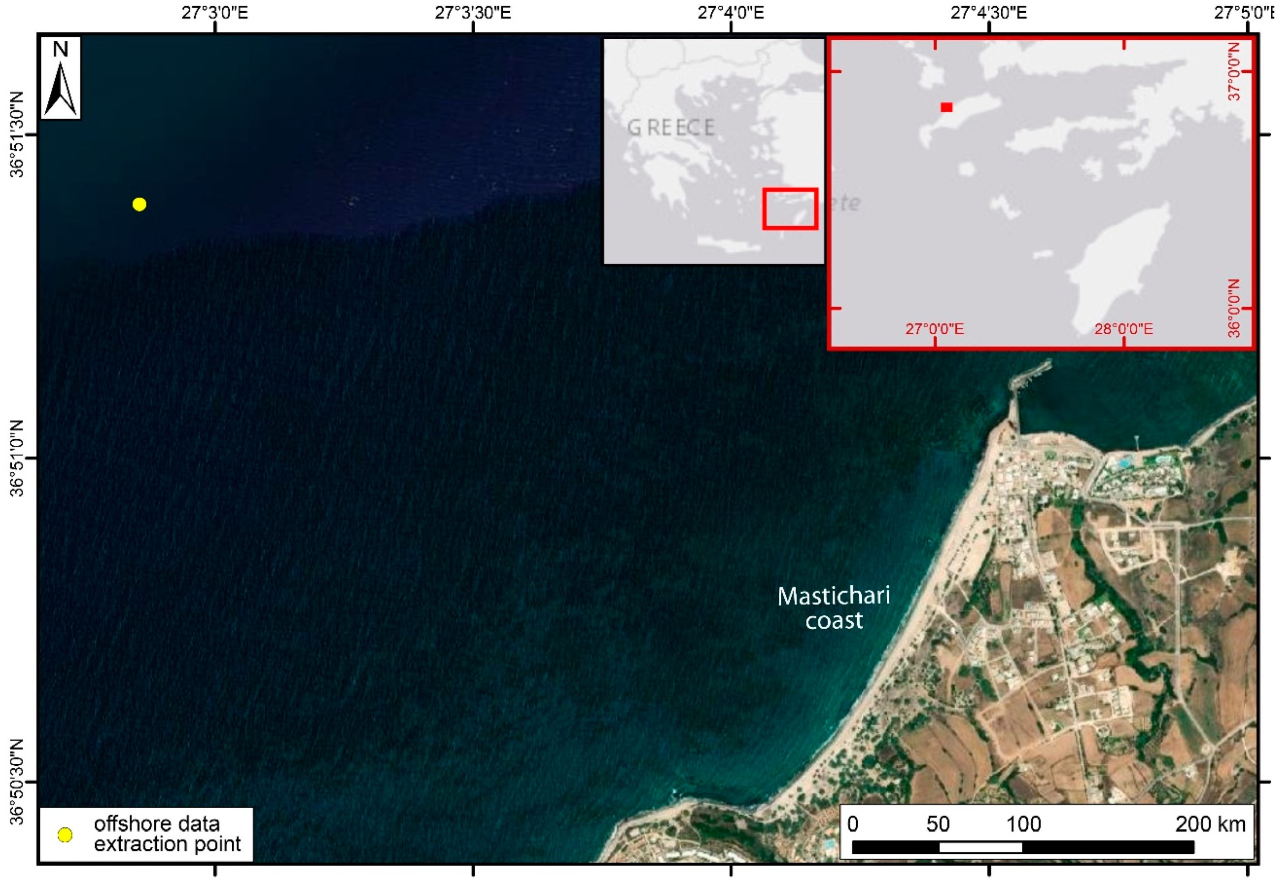
The area of interest is the sandy beach of Mastichari, which is located on the northwest coast of Kos Island (
Figure 1) in the southeast of the Aegean Sea, Greece. The coastline of Mastichari beach is northwest-oriented (
Figure 1), and it has a length of approximately 2 km. It comprises mainly of fine sand with a median diameter of 0.2 mm, which is used as an input parameter for the sediment in our simulations. At a distance of 4 km from the coast, the depths reach up to 45 m. The Mastichari beach and its surroundings have been a target of tourist activities since 1970. The small port in the northeastern side of Mastichari beach offers a frequent ferry service to the island of Kalymnos, which is opposite to it, and it is about 7.8 nautical miles away.
The beach of Mastichari is selected as a case study for the estimation of the long-term coastal evolution, since it combines a variety of properties that makes it suitable for these kinds of applications. Particularly, it consists mostly of fine sand, it has a wide nearshore zone, and it is exposed to wave conditions that attack the beach from a wide range of directions.
2.2. Bathymetry and Topography
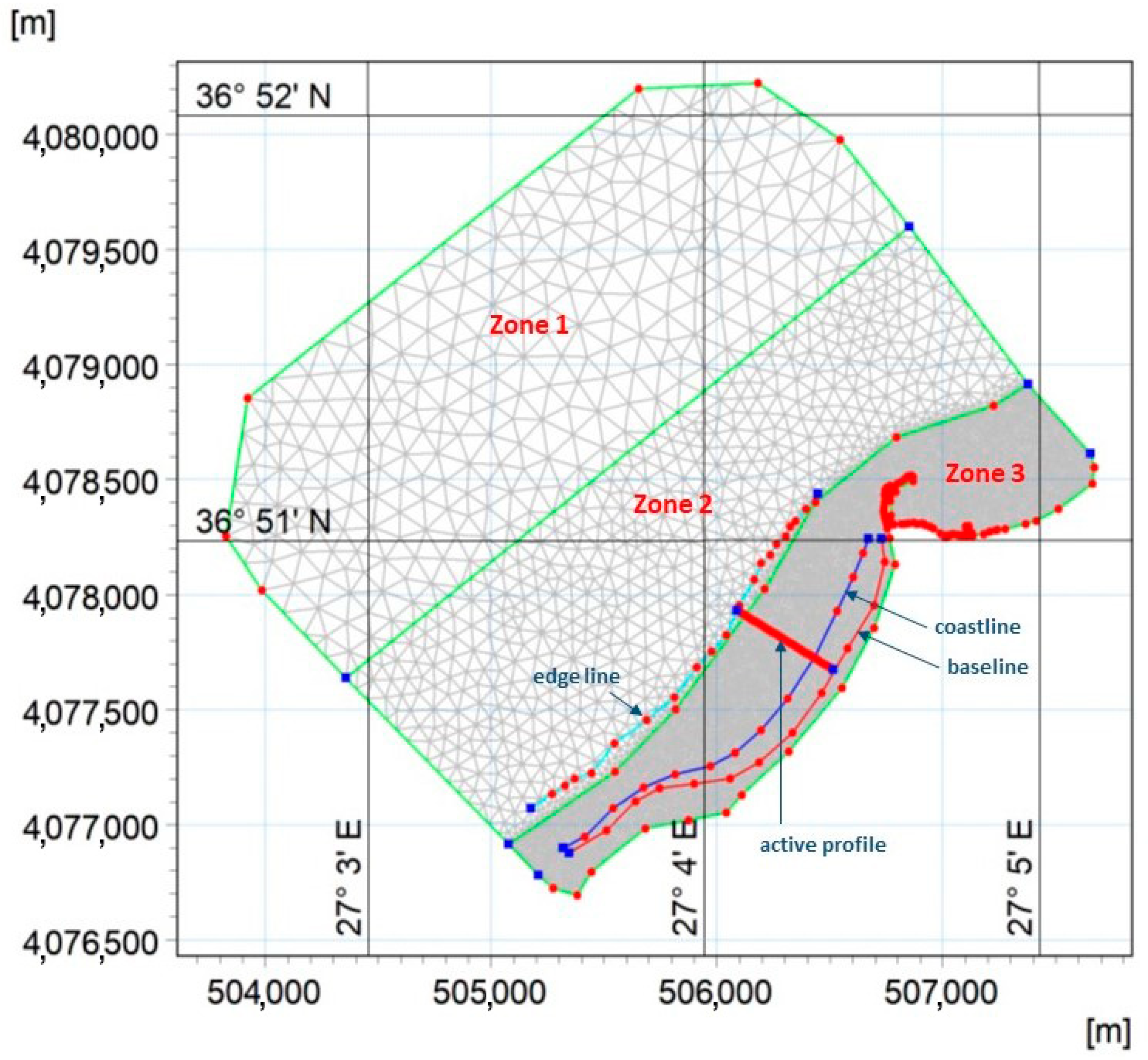
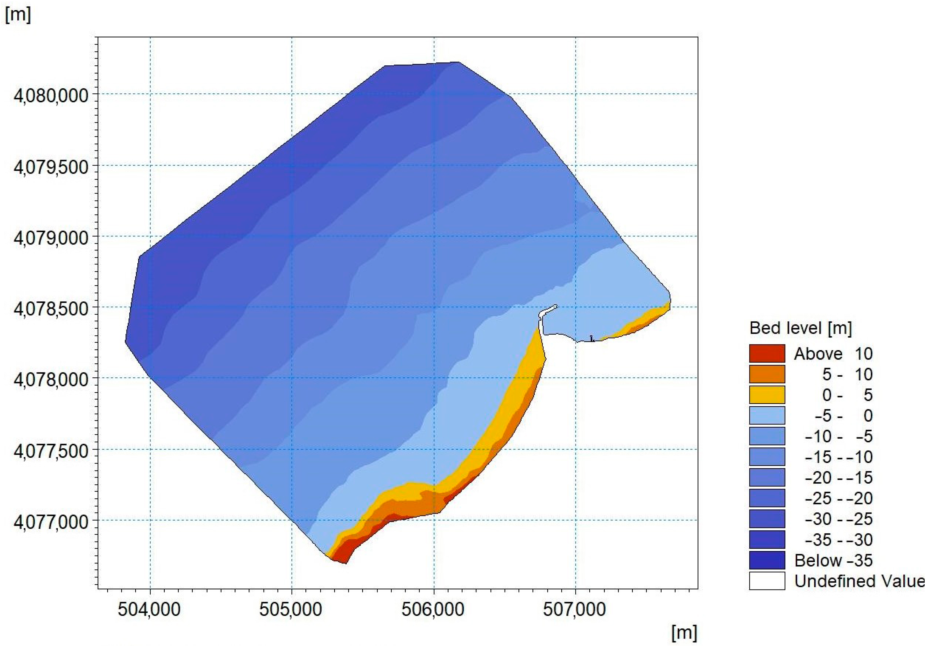
In order to simulate the morphological evolution of the sea bottom and shoreline of Mastichari coast, an unstructured finite element mesh has been constructed. Three mesh density levels are applied, with a coarser area (
Figure 2, Zone 1) being near the offshore boundary, a denser one (Zone 3) in the shallow and shoreline area, and an intermediate one (Zone 2) is implemented in the area between the other two mesh density level zones. Additionally, a high resolution (5–20 m) mesh has been applied within the closure depth and the shoreline to allow us to obtain high-resolution, significant bathymetric features in the coastal waters, while a coarser grid resolution (up to 250 m) has been applied offshore to reduce the computational cost. The intermediate mesh density level has a medium resolution (20–100 m). Additionally, a filled contour map of the bathymetry and topography information in the computational domain is presented in
Figure 3.
Water depth data have been collected during two oceanographic surveys of the R/V Alcyon (H.C.M.R.) in 2019 and 2021. During the cruises, the data were acquired in real-time by an RTK GPS system, achieving horizontal and vertical accuracies of less than 10 cm concerning the local reference GPS station. The multi-beam survey was conducted by a Teledyne Seabat T50 echo sounder following the Special Order standard of IHO. The tidal range was less than 24 cm, while the sound velocity along the water column varied between 1515 and 1522 m/s. The collected data (water depths of 7–40 m) were post-processed by the Teledyne Reson PDS-2000 software package, including the removal of spurious soundings, noise filtering, and tide and sound velocity profile corrections, and a digital terrain model (DTM) with a 2 m cell size was produced. The shallow waters (depths of 0.5–10 m) were collected along 125 nm tracks using a single beam echo sounder (Humminbird HELIX 9 CHIRP SI GPS G2N) operating in the frequency of 200 kHz. The acquisition step was one sounding per second (~195,000 soundings), and the horizontal accuracy was 2.5 m.
The Hellenic Cadastre provided a 2 m cell size elevation gridded dataset of the terrestrial part of the coastal area [
25]. Both bathymetric and hypsometric data were reprojected in ETRS89/UTM zone 35N (EPSG:25835) and resampled in the resolution of 5 m by using a Geographic Information System Software Suite (ERSI ArcGIS
®,v.10.8).
It is noted that the foreshore of Mastichari beach consists mainly of sand, while the small port of Mastichari is constructed of rocks and concrete materials. Therefore, the port has been excluded from the computational domain, and it has been set as a “hard” land boundary since it cannot be altered due to coastal processes.
2.3. Wind and Wave Climate
The time series of the wind and wave data used for the current analysis are obtained from the reanalysis dataset of ERA5 hourly data at single levels from 1959 to the present day [
26], and these were downloaded from the Copernicus database (
https://cds.climate.copernicus.eu/ accessed on 5 December 2022). The wave and wind reanalysis data used in the present paper cover the annual period from 1 January 2021 to 31 December 2021 (see
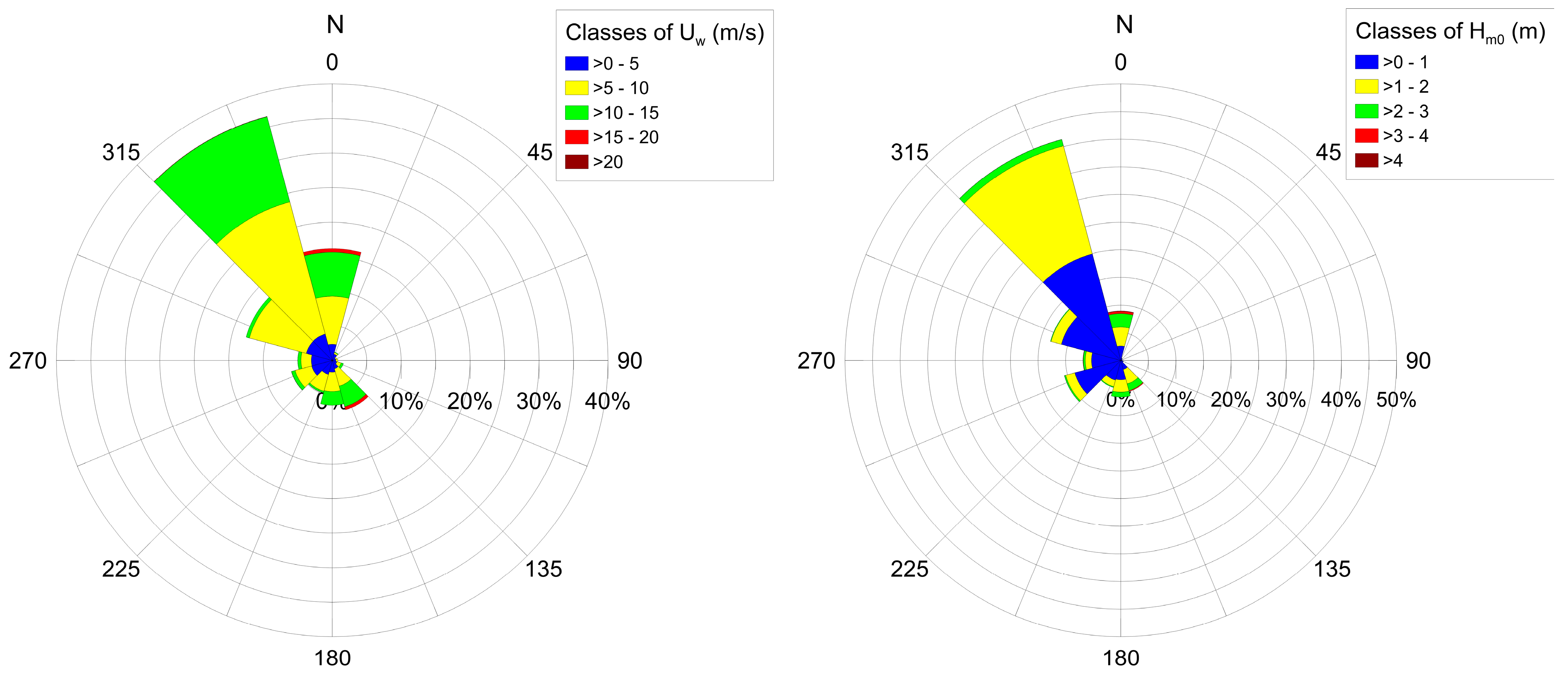
Figure 4), and the offshore wind and wave data extraction point have the spatial coordinates of 36°51′23.5″ N, 27°02′51.2″ E (see
Figure 1). The time resolution of the reanalysis data is 1 h, while the spatial resolutions are 0.25° × 0.25° (atmosphere) and 0.5° × 0.5° (ocean waves).
The prevailing winds come from the NW direction, and they usually have an intensity of 10–30 knots (for 75% of the winds), while the waves usually come from the NW direction, having an average significant wave height of about 1.0 m and a maximum value of 2.8 m. The strongest winds and waves come from north, and they are rarer than the mild wind and wave conditions. Moreover, the waves coming from north have an average significant wave height of 1.4 m and a maximum value of 4.3 m.
2.4. Wave Input Reduction Techniques
Since the objective of the present study is the long-term (≥1 year) simulation of the coastal morphodynamics due to wind-generated waves, wave climate schematization techniques have been adopted and applied. For this purpose, the time series of the offshore spectral wave data, namely, the significant wave height , the peak wave period , and mean wave direction (), are used as input data for the process-based numerical modelling.
First, the available wave time series are filtered, excluding the sea states that propagate out of the computational domain, namely, the coastal area of interest, and also those having an
lower than 0.5 m. This 0.5 m threshold is applied based on earlier simulations by the authors, showing that wave heights of less than 0.5 m cannot contribute in the sea bottom evolution of the study area, which is in agreement with [
1,
2,
27]. Therefore, this filtered time series of the triplets’
,
, and
comprises the reference wave climate, e.g., of 1 year.
2.4.1. The Energy Flux Method
After the derivation of the reference wave climate, a well-known and widely accepted wave input reduction technique, the energy flux wave schematization method [
1,
28], has been applied that separates the “equal energy flux intervals” of the reference wave climate.
The wave energy flux of each wave record in a time series is calculated via the following equation:
stands for the wave energy flux, is the seawater density (1025 kg/m3), g is the gravity acceleration (9.81 m2/s), is the significant wave height of the wave record, and is the group wave celerity in deep water, which is estimated as , depending on the of the wave record.
In order to accelerate the long-term morphological evolution simulations, the energy flux method divides the wave climate into wave classes (e.g., twelve wave bins with four directions and three height classes). It is noted that each wave class is then represented by one wave condition, which has a duration that is equal to the sum of the frequencies of occurrence of all the wave conditions that belong in the class. Each representative wave condition corresponds to the mean values of , , and of all the wave conditions of the class. Furthermore, by imposing a MORFAC, the duration of each representative wave scenario is further reduced. The reduced duration is the actual duration divided by the MORFAC value.
2.4.2. A Wind and Wave Chronology-Based Input Reduction Technique
As mentioned above, the wave input reduction method [
22] uses the wind and wave chronology, extracting the time series of the wind-wave events and swell events from the wind and wave datasets. Specifically, this method results in a time series of events of different wave intensities and durations. Moreover, it can accelerate the estimation of the long-term coastal morphodynamics by using a MORFAC.
To accomplish the greatest acceleration by applying this method, the time series is shortened so that a uniform MORFAC value is imposed. In particular, the initial durations of the events are divided by the MORFAC value to estimate the new durations. It is noted that the time step of the input time series can be variable, and it does not have to be the same as the time step of the hydrodynamic simulation since a type of interpolation can be applied [
29].
To describe the wave chronology-based input reduction technique, the swell criterion is initially applied to the datasets according to the Thompson et al. [
30] classification that separates swell seas from wind seas. This criterion is implemented because the two wave types have distinct characteristics [
31], which in turn, produce different effects on the sea bottom and the beach profile. Wind seas usually have an offshore peak wave steepness that is higher than 0.025. This steepness is defined as the ratio of the offshore significant wave height (
) and the wavelength (
) based on peak wave period
. The swell steepness diminishes as the waves move away from the fetch region [
32]. Swell seas with steepness values of 0.010–0.025, 0.004–0.010, and <0.004 are classified as young, mature, and old ones, respectively.
Additionally, since the sea bottom morphological changes are mainly caused by wave-induced currents and short-crested waves generated by wind, the wind characteristics and their time history can be used to extract representative wave scenarios for wind seas. The primary aim of the present analysis is the derivation of wind-wave events that are defined here as the consecutive wave data of wind seas corresponding to the approximately constant wind. It is noted that these wind-wave events could be of different types, such as fetch-limited or duration-limited growing seas, or fully developed seas (e.g., [
33,
34]). It is also noteworthy that the definition of constant wind is commonly used for the estimation and prediction of offshore wave conditions based on the wind data.
Following the above two conditions of approximately constant wind, each wind-wave event in the present study is determined by a segment of non-overlapped consecutive wind data that satisfy the statement below:
where
is the time variable,
the time interval covered by a certain wind-wave event, and where
and
are the mean values of the successive and acceptable (e.g., hourly) wind speed
and direction
data, respectively.
In the method developed in [
22], each swell and wind-wave event is represented by a characteristic wave condition. Referring now to linear data, such as the wave height and wave period, the representative wave characteristics of each wind-wave and swell event are the arithmetic mean values of the corresponding consecutive wave data, as follows:
where
, and
, are the mean values of the successive data of the significant wave heights
and the peak wave periods
included in each event, respectively, N is the number of successive data, and
is a discrete variable for time. Additionally,
is the duration of the event.
The circular variable
has been estimated by the following formula (referenced in, e.g., [
35,
36,
37]).
where
where
is the mean value of the successive data of the mean wave direction
included in each event.
The methodology of Malliouri et al. [
22] needs a wave series, but it also needs a wind time series of the same time period in order to extract a sequence of wind-wave and swell events, which implies a limitation regarding the properties of the used source data. Except for this, it would be an advantage if the wave events could be derived from the wave time series only since the main objective of the present paper is to estimate the wave-induced coastal mophodynamics.
2.4.3. A Wave Chronology-Based Input Reduction Technique
The lack of current studies which thoroughly consider the wave chronology in wave input reduction techniques creates the necessity to develop a novel and easy-to-use methodology for extracting the time series of wave events of different wave intensities and variable time intervals (meaning durations). This method derives those wave events sequences exclusively from the time series of wave data, irrespective of the type of wave events (wind-wave, young, mature, or old swell ones), by applying three specific conditions.
Following the three conditions of similar consecutive wave characteristics, each wave event in the present paper is determined by a segment of non-overlapped successive wave data which satisfies the statement noted below:
where
is the time variable,
is the time interval covered by a particular wave event, and
,
, and
are the maximum acceptable values of the absolute differences of
,
, and
from their mean values
,
, and
, respectively.
The values of the , , parameters are determined after conducting earlier simulations runs using the MIKE 21 Coupled Model FM software package and by using the events parameters , , and as input data, while attempting to find an equilibrium solution between the need to increase the duration of the wave events to accelerate the process by using a high MORFAC value and the accuracy limitation. The latter one requires that each wave event should be comprised of consecutive wave data of similar wave characteristics so that they can be properly represented by one wave condition.
From a statistical point of view, specific , , and values are selected based on the degree of variability of the wave data of the derived events with respect to their mean wave characteristics. It is expected that lower , , and values imply less dispersed wave data for the corresponding events, namely, lower coefficients of variation. Moreover, the fact that uniform , , and values are applied for the whole time series, irrespective of the wave intensity of each wave event, necessitates that the resulting coefficient of variation of the produced events, and especially their values, are not correlated to a significant degree.
2.4.4. Simulations
Using all the above information, the following six simulations have been performed:
A simulation consisting of the full time series at the offshore boundary, which is denoted as the reference/benchmark simulation.
Five repetitive simulations using the 12 representatives in random order, which were calculated by the energy flux input reduction method and are denoted as the energy flux simulation with five repetitions. The average of 5 repetitions is in accordance with [
4], the authors of which used the same approach for estimating the average performance score of the Energy Flux Method. In this study, the average result of the 5 repetitions was estimated as the expected result, considering the uncertainty of the random order of the 12 representative scenarios and its effect on the final result.
A simulation consisting of a time series of representatives of wind-wave events and swell events, which have been extracted by the wave input reduction technique of Malliouri et al. [
22], which is denoted hereafter as the wind and wave chronology- based input reduction technique.
A set of three simulations consisting of isolated sequences of the representative scenarios of wave events with similar characteristics based on the three criteria (see Equation (8)) for specific , , and values and specific morphological acceleration factors (MORFAC), which are denoted hereafter as the wave chronology- based input reduction techniques.
2.5. Numerical Model Setup
The process-based numerical model used in the present study for the detailed description and estimation of the hydrodynamic conditions, waves, sediment transport, sea bottom and shoreline evolution on the beach in Mastichari is the MIKE 21 Coupled Model FM [
29]. The same numerical coupled model has been applied in a plethora of relevant recent studies such as [
2,
38,
39,
40,
41].
The MIKE 21 Coupled Model FM software package is composed of several interrelated modules, and four of them have been implemented in the present study: (i) the hydrodynamic (HD) module, (ii) the spectral wave (SW) module, (iii) the sand transport (ST) module, and (iv) the shoreline morphology module (SM). SW is a 3rd generation spectral wave model that simulates the growth, decay, and transformation of wind-generated waves and swell in offshore and coastal areas. HD is a depth-averaged hydrodynamic model that uses the Navier–Stokes equations of motion, and it is suitable for the estimation of the nearshore circulation. Moreover, ST is a sand transport and morphology dynamic model that is used to calculate the transport of non-cohesive materials based on the mean horizontal flow conditions assessed in the HD module. Furthermore, the SM module is a complementary module that can be included in ST module during dynamic numerical modeling. SM combines a one-line model for the shoreline with a 2D model for the wave, current, and sediment transport. The incorporation of SM for the long-term estimation of sea bottom evolution eliminates the effect of cross-shore transport on the morphology, thereby increasing the stability for long-term simulations. Without this module (SM), the ST module updates the bottom level of each mesh element based on the local sediment continuity equation, which could lead to instabilities in the long-term simulations.
Focusing on the SM module in the present paper, the combined 2D and shoreline morphology option, which is defined by an active profile, has been selected to be used in the morphological calculations. Particularly, the SM module solves a modified version of the one-line equation for the shoreline (see [
42]), whereby the direction of the shoreline is transformed to be perpendicular to the local orientation of a baseline. The baseline is defined by a set of points forming a polyline (see
Figure 2), the position of which is fixed, and the local orientation of the baseline is defined by the user during the model setup.
Additionally, the coastline (see
Figure 2) defines the initial position of the local shoreline, which is subject to erosion and deposition. The grid points along the coastline represent a shoreline edge that can move onshore and offshore. The sediment volume deposited on the strip of the foreshore zone and within the active profile will contribute to the movement of the shoreline edge. The profile defines a representative cross-shore profile that moves forth and back with the shoreline edge at the given location. It is noted that two parameters are predefined concerning the active profile; these are the closure depth and the shoreline’s top elevation level. This means that when the shoreline erodes, the elevation level of the 2D computational domain will decrease accordingly, including any section of the profile that is above the top elevation level, but it will not include those that are below the closure depth. Moreover, when the shoreline is subject to accretion, the elevation level of the 2D computational domain will increase accordingly, including any section of the profile that is below the closure depth, but it will not include those that are above the top elevation level [
29].
In our case study, the closure depth is estimated by Houston’s approach [
43] at 6.2 m. The top z-level coincides with 1.6 m, which is the average, maximum active beach height of several profiles perpendicular to the shoreline in the study area. This is considered to be the limit of the permanent vegetation or the limit of the constructions. The depth of closure is the seaward limit of the active coastal zone, of which there are no significant sea bottom morphological changes and no significant net sediment transport which occurs between the offshore and the nearshore. Both the closure depth and the top elevation of the active coastal zone are site specific.
In the reference simulation from 2021 and the Energy Flux Method simulations, the applied time step is 1 h, but they have different MORFAC values. As for the wind and wave chronology-based reduction method and the wave chronology-based ones, they all are combined with the time step (
) of 1800 s (see
Table 1). The time step in these cases is lower than those in the first two simulations due to the fact that the event time series have a non-equidistant calendar axis and also because the events have variable durations, which are not necessarily multiples of MORFAC. Additionally, in this way, the coastal morphology has milder alterations from one time step to another than those in cases of larger times steps, thus increasing the results’ accuracy and the simulations’ stability. Referring to the wave chronology-based input reduction technique, three simulations are presented here. In the first one, relatively low values of the
,
, and
parameters are combined with a MORFAC of 5, while in the other two cases, higher values of these three parameters, as well as of the MORFAC values, are utilized (see
Table 1).
It is noteworthy that various MORFAC values have been derived after the statistical analysis of the wave events based on the
,
, and
criterion and depending on the events’ frequency of occurrence in the examined period. Particularly, the
,
, and
values determine the derived events’ duration, as well as the coefficient of variation of the events’ data and the accuracy of their representation by the mean values. However, the MORFAC value determines the degree of reduction of the model run time and the accuracy of the results [
6,
7].
It is noteworthy that the time step mentioned above () in each of the various modules is an overall time step. Specifically, the hydrodynamic, the sand transport, and the spectral wave calculations also use internal time intervals, which are dynamic and determined in order to meet the stability criteria (e.g., the Courant stability condition).
2.6. Evaluation of Wave Input Reduction Techniques
The results obtained by implementing the alternative wave input reduction techniques and the process-based model MIKE21 Coupled Model FM are compared. In order to evaluate the performance of these techniques, the most commonly used criterion (e.g., [
44,
45]), the Brier Skill Score (
), is calculated for each method via the following relationship:
where
denotes the estimated, modelled output quantity,
denotes a measured quantity corresponding to the benchmark wave climate simulation for the present study, and B is a baseline prediction, usually referring to the initial bathymetry, assuming that there is no sea bottom alteration. Moreover, the square brackets denote average quantities over the whole computational domain.
Following Sutherland et al. [
45] (2004), in order to evaluate the performance of a specific morphological evolution model, a classification is proposed for the
, i.e., an excellent performance corresponds to a
range that is between 0.5 and 1, while good, reasonable, poor, and bad performances correspond to
ranges of (0.2, 0.5), (0.1, 0.2), (0, 0.1), and <0, respectively.
3. Results
3.1. Representative Wave Conditions
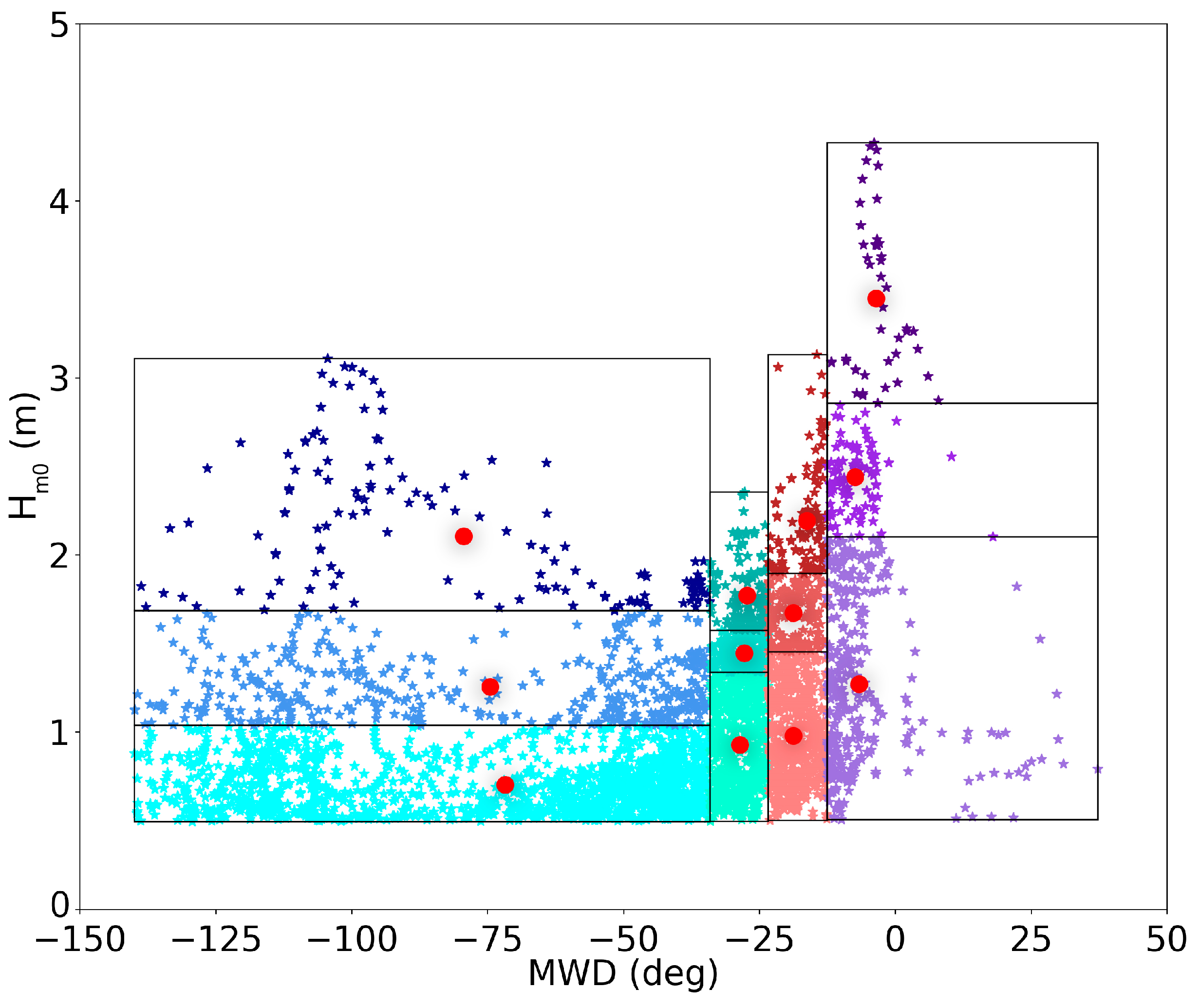
The 12 representative scenarios of the 12 bins of the Energy Flux Method are derived in order that all the bins have equal energy fluxes, which are estimated as the sum of the energy flux of each bin’s included sea states, regardless of the sea states’ chronology. Each representative wave condition (red circles in
Figure 5) corresponds to the mean values of
,
, and
of all the wave conditions of the class. As it can be seen, the bins, including the highly energetic sea states, tend to include fewer wave conditions in the class. Furthermore, in contrast to the Fixed Bins Method, the bins of the Energy Flux Method have unequal sizes.
In addition to the Energy Flux Method, the wind and wave chronology-based reduction technique has also been applied, which produces the time series with a larger number of representative wave events (see the rhombus in
Figure 6) than that of the Energy Flux Method. These wave events preserve the original sequence of the sea states. They are either swell events, which have been extracted based on their wave steepness, or wind-wave events, whose data follow the condition of approximately constant wind. The estimated swell events can consist of swell data of different characteristics, while the wind-wave events consist of more similar wind and wave characteristics.
As for the chronology-based wave input reduction method, the number of the estimated wave events in the first 120 h, presented in
Figure 6, varies between 10 and 38, with the smallest number occurring in the case of the largest values (
= 0.8 m;
= 1.5 s;
= 20 deg.) and the largest number occurring in the case of the lowest (
= 0.2 m;
= 0.5
s;
= 10 deg.) applied maximum acceptable values of the absolute differences between
,
, and
and their mean values
,
, and
, respectively. In the case of the medium applied values for the
,
, and
parameters, 16 wave events are extracted in the first 120 h.
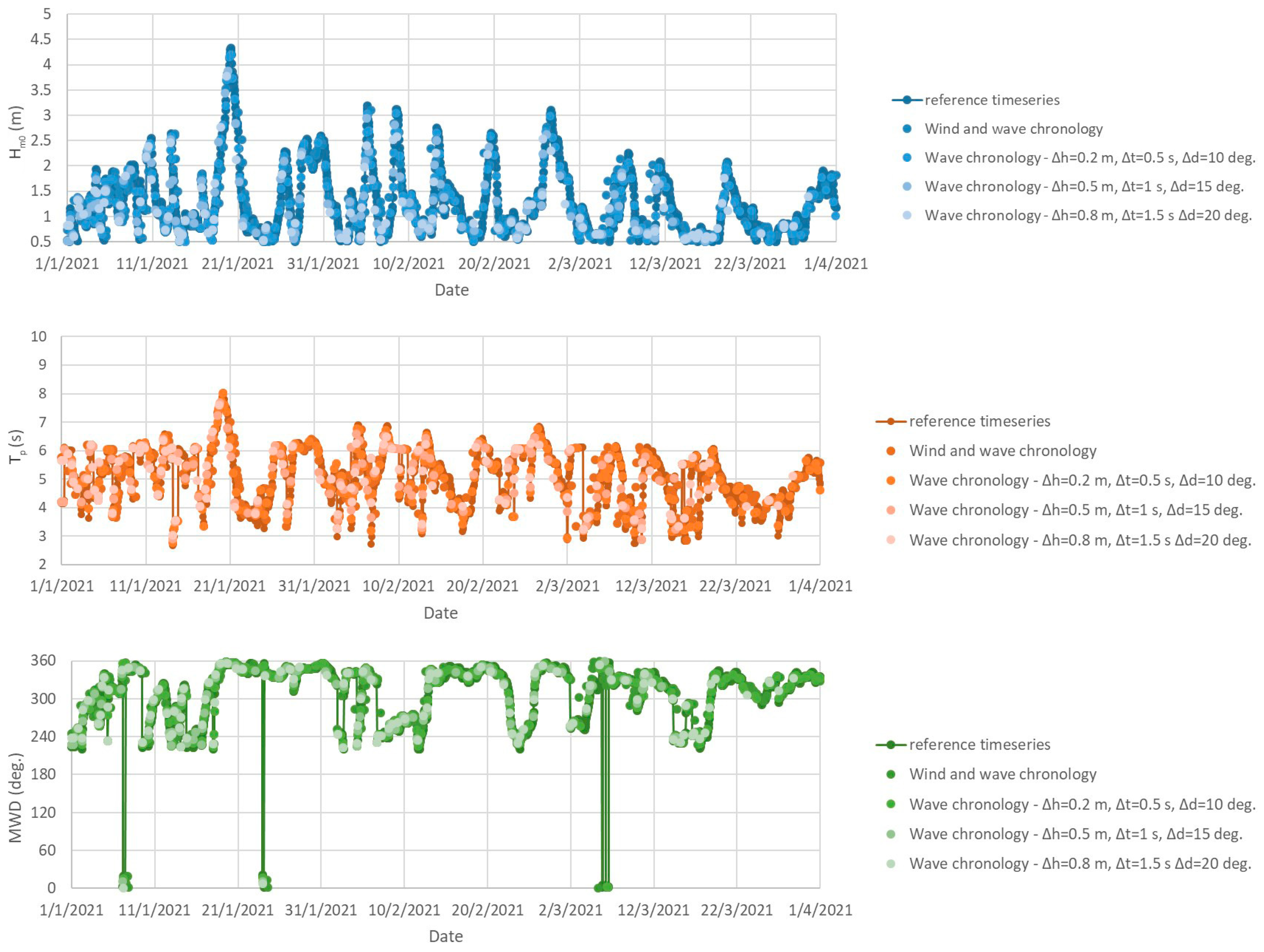
In a larger subset of the time series, e.g., 3 months of 2021 presented in
Figure 7, than that in
Figure 6, all the applied chronology-based simulations seem to follow the time series concerning
,
, and
, and similar differences are observed in terms of the number of the extracted events and their durations.
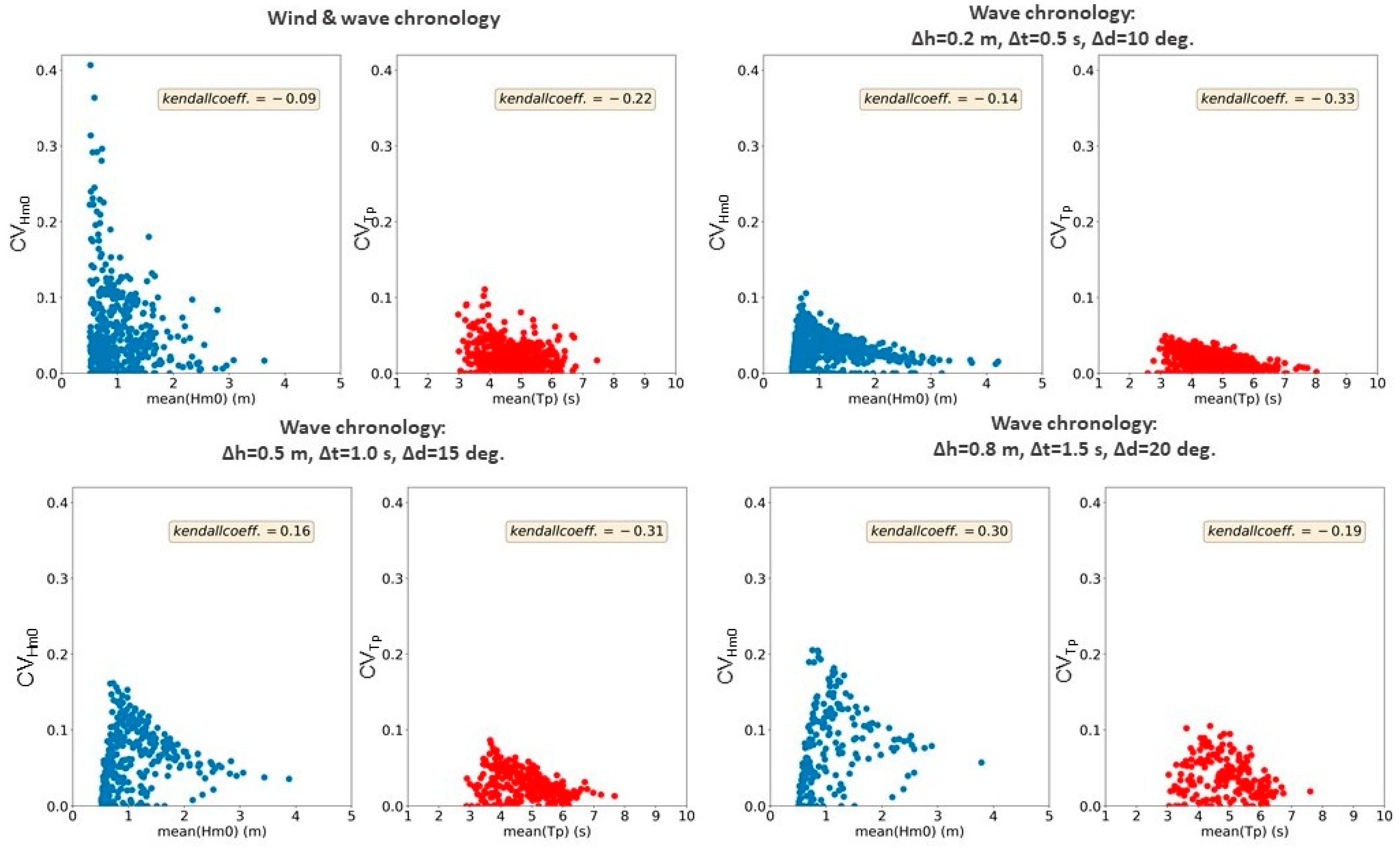
At this point, the dispersion of the wave data within the related events is estimated for the four chronology-based reduction techniques. Particularly, the coefficients of variation (CV), i.e., the standard deviations of
and
of the produced wave events’ data from their mean values, are displayed in
Figure 8, showing that higher
,
, and
values allow for greater dispersion, and vice versa. In the reduction technique that uses the wind and wave chronology, the CVs of
are less than 0.4, while for
, they are less than 2 m, and they are lower than 0.025 for the
and greater than 3 m. The wave chronology-based reduction technique using
= 0.2 m,
= 0.5 s, and
= 10 deg. produced the lowest dispersion of the wave data, with CVs that are lower than 0.1 for
, less than 2 m, and lower than 0.025 for
, and they are greater than 3 m. Moreover, the wave chronology-based reduction technique with the intermediate
,
, and
values has CVs that are lower than 0.18 for
, less than 2 m, and lower than 0.05 for
, and they are greater than 3 m, while the one with the largest
,
, and
values has CVs that are lower than 0.21 for
, less than 2 m, and lower than 0.08 for
, and they are greater than 3 m.
In addition to , the coefficient of variation of is also calculated, presenting similar behavior, but not to the same extend as that for . Specifically, the dispersion of the data in the produced events is usually lower than that of in the four cases. Additionally, the estimated Kendall correlation coefficient presents a degree of dependence between the CVs of and and their mean values. The Kendall correlation coefficient of the CVs of and varies from −0.09 to 0.30 for the four techniques, whereas the one that corresponds to lies within the range from −0.33 to −0.19. Thus, it does not show a high degree of dependence between the corresponding elements in the four cases.
3.2. Numerical Models Results
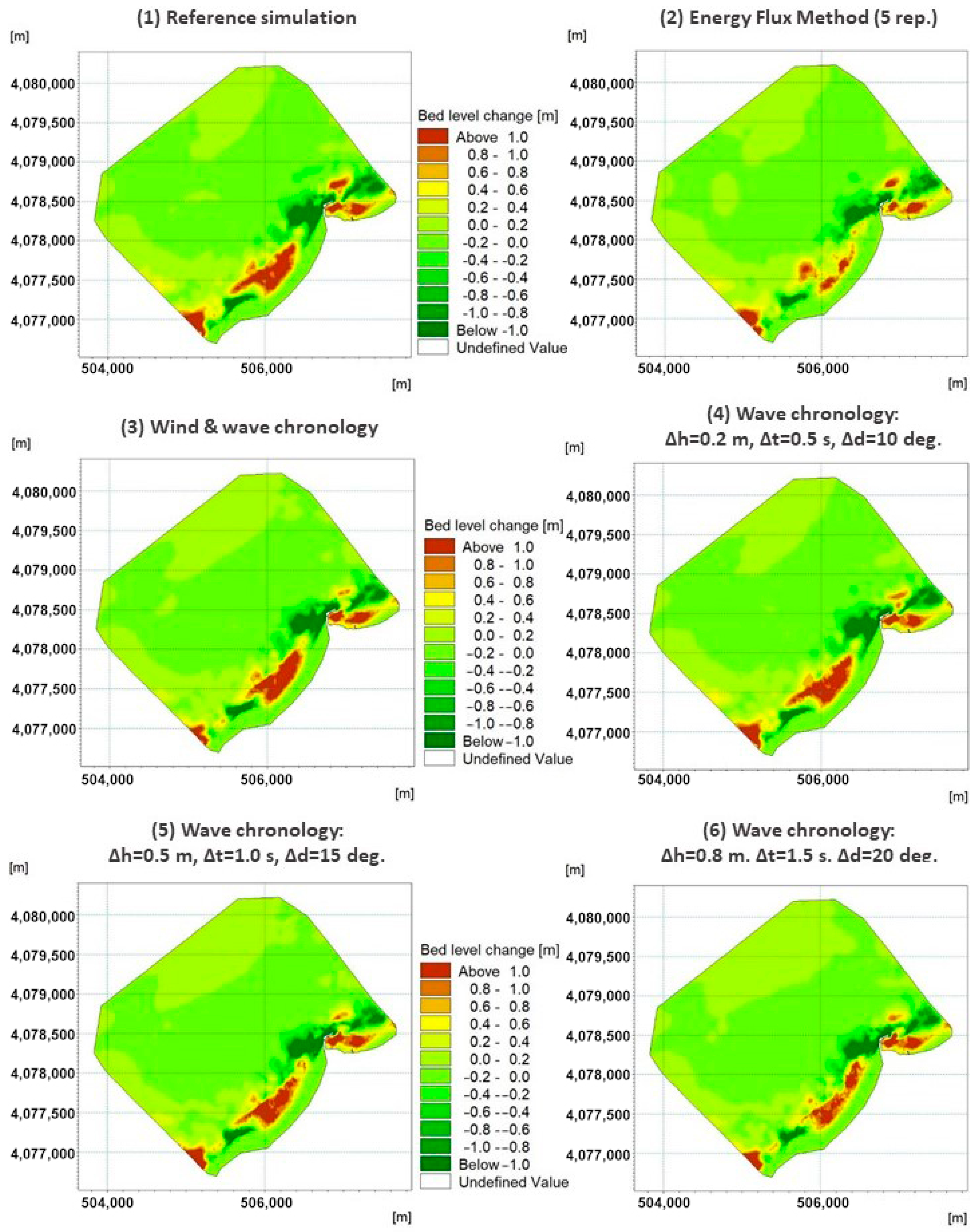
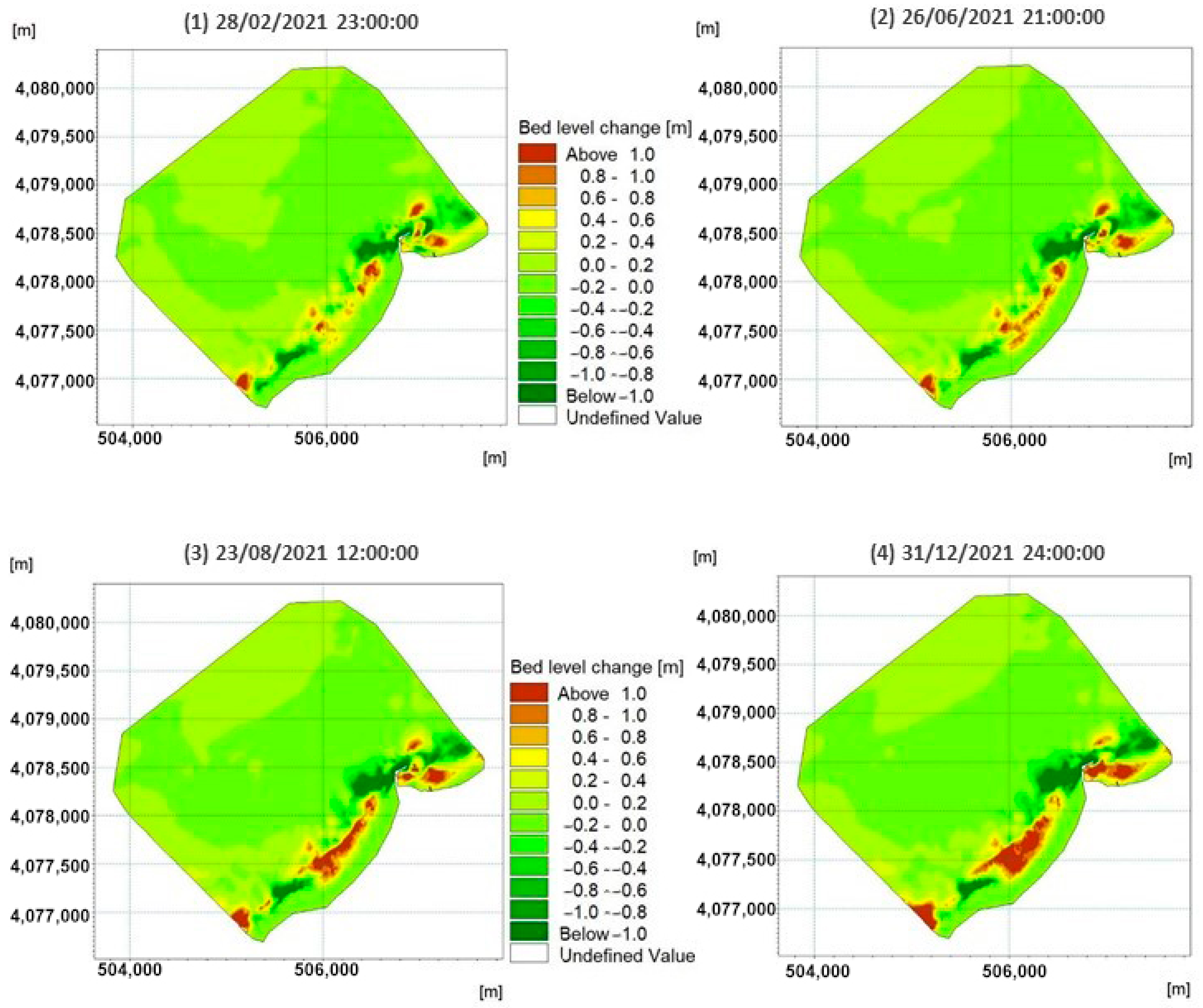
The present section presents the morphological bottom and shoreline evolution of the area of interest using the dataset of 365 days (see
Figure 9). The first simulation that is displayed in
Figure 9 is the benchmark one, which is used to validate the wave chronology-based input reduction methods developed in the present paper. The most dominant wave direction turned out to be the northern one, as shown by the representative wave conditions in
Figure 4 and
Figure 5. Consequently, the prevailing longshore sediment transport’s direction is from northeast to the southwest, as shown in
Figure 9, resulting mainly in accretive patterns on the beach face from the center of Mastichari beach to the southwest cape. Additionally, erosion patterns are observed in the shoreface and the sea bottom in front of the port structure within 450 m southwest of the port of Mastichari. The mean values of the sea bottom evolution are estimated to be −2.1 m and 1.1 m in the erosion and accretion areas, respectively.
The second one is the average simulation based on the Energy Flux Method used to conduct five repetitions of the 12 characteristic scenarios’ random sequences. In the energy flux simulation, the predicted bottom evolution in the area of interest is of a lower order than that of the reference simulation. Precisely, the mean values of the sea bottom evolution are estimated to be −1.6 m and 0.8 m in the erosion and accretion areas, respectively. Additionally, the erosion area has a shorter length on the beach face than it does in the reference simulation, namely 280 m, while in the reference simulation, the erosion pattern has a length of 450 m.
Regarding the third simulation based on the reduction method that uses the wind and wave chronology information, the erosion and accretion patterns have similar extends to those of the benchmark simulation. In particular, the mean values of the sea bottom evolution are estimated to be −1.9 m and 1.0 m in the erosion and accretion areas, respectively, and the erosion area has a length of 420 m in front of the shoreface near the port structure.
In the fourth simulation, corresponding to the lowest applied values of the , , and parameters, the predicted bottom evolution of the key study is of the same order as it is in the reference simulation. Precisely, the mean values of the sea bottom evolution are estimated to be −2.0 m and 1.0 m in the erosion and accretion areas, respectively. Additionally, the erosion area has the same extent as it does in the reference simulation. In the fifth simulation, i.e., the one with the medium values of the , , and parameters, the predicted bottom evolution in the area of interest is again of the same order as that of the reference simulation. However, the erosion area has a slightly shorter length of 405 m in front of the beach face near Mastichari port. Moreover, the mean values of the sea bottom evolution are estimated to be −2.0 m and 1.0 m in the erosion and accretion areas, respectively. In the sixth simulation that uses the largest applied values of the , , and parameters, the differences are greater than those in the benchmark simulation. The erosion area in the sixth simulation has the smallest length among the other five simulations, which is estimated to be 210 m, and the mean values of the sea bottom evolution are estimated to be −1.7 m in the erosion area and 0.8 m in the accretion area.
Referring at this point to the model’s run-time, the run-time reduction, as well as the Brier score (see
Table 2), the benchmark simulation has the longest duration of 14.65 h, the wave input reduction simulation with the shortest duration (3.23 h) is the sixth one, but it has the lowest
value. Additionally, the wave input reduction simulation with the largest duration (8.42 h) is the sixth one, and it has the highest
value. The other acceleration techniques’ simulations have intermediate
values, and they achieved moderate model run-time reductions than the already mentioned ones did.
4. Discussion
As far as the obtained representative wave scenarios of the wave input reduction techniques are concerned, a total of 12 representative wave conditions (see
Figure 5) for the Energy Flux Method are selected to represent the data of 1 year (1 January 2021–31 December 2021), following [
1]. It is noted that in order to limit the effect of the random initial choice on the performance of the technique, i.e., on the accuracy of the morphology prediction, five replicates [
3,
4] of the random sequences of the twelve wave scenarios are applied, displaying the average result (see
Figure 9 (2)). This is in compliance with [
16], which estimated the average skill score of the five repetitions in order to assess the performance of the binning methods.
Nevertheless, in the above method, which is the most commonly used one for long-term coastal zone evolution studies, the wave chronology is not considered in detail, and the evolution of sea bottom, coastline, and shoreline are not predicted as a function of time. Therefore, the results are obtained at the end of long time intervals, e.g., of 1 year, (e.g., [
1,
3,
4,
21]). Hence, in order to tackle the lack of estimations of the evolution of coastal morphology as a function of time and the need to accelerate this process, two methodologies are described in the present study for extracting the time series of wave events of different wave intensities and variable durations. The first one is the wave input reduction method by Malliouri et al. [
22] that extracts the sequences of wind-wave events and swell events from wind and wave time series (see
Figure 6 (up)). In the second one, wave events sequences are exclusively derived from wave time series (see
Figure 6 (below)), irrespective of the type of wave events (wind-wave, young, mature, or old swell ones), by applying three specific conditions.
The two methods thoroughly consider the wave chronology or wind and wave chronology, producing time series of the sea bottom and shoreline evolution. This information is vital for assessing the coastal zone evolution as a function of time, e.g., before and after extreme coastal storm events that can induce severe sea bottom and shoreline changes, but also during mild weather conditions that can result in the recovery of the beaches. Moreover, the two methods could also predict sea bottom and shoreline evolution in the future if they are applied to climate data of future projections, and thus, they could be used for coastal zone monitoring.
Additionally, the reference time series and the wave events time series extracted by the four chronology-based reduction techniques’ time series, namely, the wind and wave chronology-based input reduction method and the three wave chronology-based input reduction methods with different values for the
,
, and
parameters, are compared in terms of specific time periods (
Figure 6 and
Figure 7).
Through these comparisons, it is observed that the lower the , , and values are, the less data that are reduced, albeit the time series of the obtained wave events tend to represent the benchmark time series more accurately than the other methods do, and vice versa. As for the wind and wave chronology-based input reduction method, its produced time series does not precisely follow the benchmark time series. This is probably due to the complexity of nature that makes the assumptions adopted somewhat simplified, i.e., that the approximately constant wind corresponds over time to approximately constant wave conditions. To be more specific, the observed offshore wave conditions can be a combination of a variety of generating factors, e.g., wind coming from multiple directions and swells of different age classes. Moreover, grouping consecutive swell data by one swell event implies another simplification, since they might have different characteristics or come from different weather systems.
The obtained process-based numerical model results acquired by using the benchmark simulation are then compared with the wave input reduction methods’ simulations regarding the methods’ performance, meaning the accuracy of their results in combination with the acceleration of the model run, namely, the reduction of the model run-time. A significant advantage of the wave and wind or wave chronology-based wave input reduction techniques compared to those techniques that do not consider wave chronology is that the first ones can estimate sea bottom and shoreline evolution as a function of time (see
Figure 10). This information could illuminate the path for the accurate forecasting of coastal evolution and coastal monitoring.
The accuracies of the different techniques are evaluated through the Brier Skill Score (
), which is calculated for each method (see
Table 2) via Equation (10). All the simulations achieved a score of “excellent” (
Table 2), according to the classification proposed by Sutherland et al. [
45]. However, some distinct differences are identified, especially in the Energy Flux Method’s results and those of the sixth simulation compared with those of the reference simulation ones. These two simulations seem to underestimate the sea bottom evolution to a greater extent than the other wave-input reduction methods do. This is attributed to the fact that the Energy Flux Method does not consider wave chronology, which is in contrast to the wind and wave- or wave chronology-based wave input reduction methods. Moreover, the sixth simulation, i.e., the wave input reduction method using the wave chronology with the largest maximum acceptable values of the absolute differences of
,
, and
from their mean values
,
, and
(
= 0.8 m,
= 1.5 s,
= 20 deg.), has the lowest
value, but this value is very close to the Energy Flux Method’s
value. This is due to the relatively large values of
,
, and
, which can result in grouping of less similar sequential wave data to the same wave events than the techniques of lower values of those parameters. From a similar perspective, the most accurate results are produced by the wave chronology based-wave input reduction method with the lowest applied
,
, and
values.
The higher accuracy of a wave input reduction method’ results is usually combined with a higher model run-time, and thus, less data reduction occurs. For example, the sixth simulation presents less accurate results despite it having an excellent value like all the other tested methods do, but it achieved the most significant acceleration of the simulation’s model run. Similarly, the fourth simulation has the longest run-time compared to those of the other wave input reduction methods, and it achieved a run-time reduction of 43%, but it presents the highest value, which is significantly high and close to unity.
5. Conclusions
The simulation of the long-term (≥1 year) morphological evolution (bathymetry and shoreline) of Mastichari beach is based on three wave climate schematization techniques used to determine the temporal succession of wind-generated waves.
The first simulation is the benchmark one consisting of the full time series of 2021. The second one is the average simulation based on the Energy Flux Method of five repetitions of the twelve characteristic scenarios’ random sequences. Additionally, the third simulation follows the wind and wave chronology-based input reduction method, whereas the fourth, fifth, and sixth ones are the simulations based on the wave chronology-based input reduction method using different values for the maximum absolute differences of , , and from their mean values , , and (, , and parameters, respectively).
In the second simulation, which uses the most common wave input reduction method for the long-term coastal zone evolution study, the wave chronology is not considered in detail, and sea bottom, coastline, and shoreline evolution are not predicted as a function of time. Therefore, the results are obtained at the end of considerable time intervals, e.g., of 1 year. On the contrary, the two new methodologies presented in the present study preserve the information about the wave chronology, extract time series of wave events of different wave intensities and variable durations, and estimate the coastal evolution as a function of time. The first wave input reduction method extracts sequences of wind-wave events and swell events from wind and wave time series, and in the second one, the wave events sequences are exclusively derived from the wave time series by applying three specific wave conditions.
All the applied methods achieve a rating of “excellent” in this case study. Nevertheless, some distinct differences are identified concerning the methods’ performance. Specifically, the Energy Flux Method’s results and those of the wave chronology-based reduction techniques with the largest values of , , an d parameters ( = 0.8 m; = 1.5 s; = 20 deg.) are the less accurate ones. However, they present a higher acceleration of the model run compared to the rest of the methods. The other three chronology-based input reduction methods have satisfactory accuracy ( value ≥ 0.85), but they have significantly different model run-time reductions. Remarkably, the highest model run-time reduction accomplished by these three methods is that of the wave chronology-based wave input reduction method with the medium , , and values ( = 0.5 m; = 1.0 s; = 15 deg.), and thus, this the one most highly recommended one. The wind and wave chronology-based wave input reduction method has slightly more accurate results than the wave chronology based on the medium , , and values does, but the model run is slower. Moreover, the most accurate method is the wave chronology-based wave input reduction method with the lowest , , and values ( = 0.2 m; = 0.5 s; = 10 deg.). However, it does not achieve the most proper equilibrium between the need to decrease the duration of the model run and to meet the accuracy limitation.
Therefore, the accuracy of the model results is a function of the , , and values and the MORFAC value. Specifically, the , , and values determine the durations of the derived events and the accuracy of the events’ data representation as per the mean values.
It is noted that higher , , and values can produce higher MORFAC values in the simulations than lower , , and values can, hence they can reduce the model run-time to a greater degree. Nevertheless, the higher these parameters are, the lower the accuracy is, and vice versa. Hence, the , , and values and the MORFAC value are interrelated, affecting both the results’ accuracy and the model run time.
In short, the new wave chronology-based wave input reduction method can produce a time series of wave events, hence it can predict coastal evolution as a function of time. The performance of this novel technique is evaluated in the present study. It is shown that it can achieve a model run-time reduction of about 70%, providing satisfactorily accurate results at the same time. This research could be useful for coastal engineering studies and for coastal zone monitoring, and it could be a reliable tool for coastal engineers and marine scientists.


 ,
, 


