
Novel Ensemble Machine Learning Modeling Approach for Groundwater Potential Mapping in Parbhani District of Maharashtra, India

 ,
, 
 , ,
, ,  , ,
, ,  ,
, 
Abstract
:1. Introduction
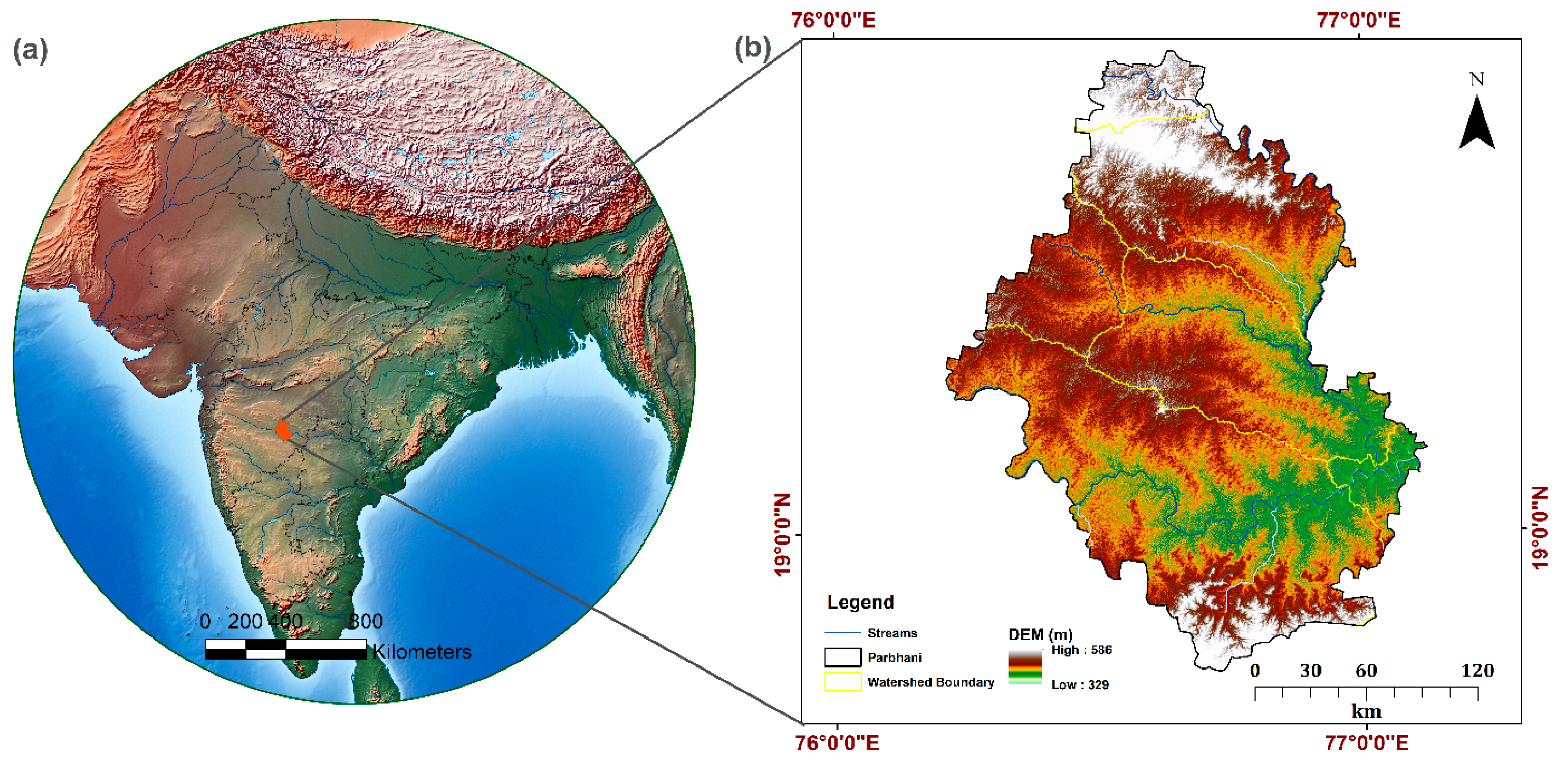
2. Site Description
3. Database and Methodology
3.1. Groundwater Potential Conditioning Factors
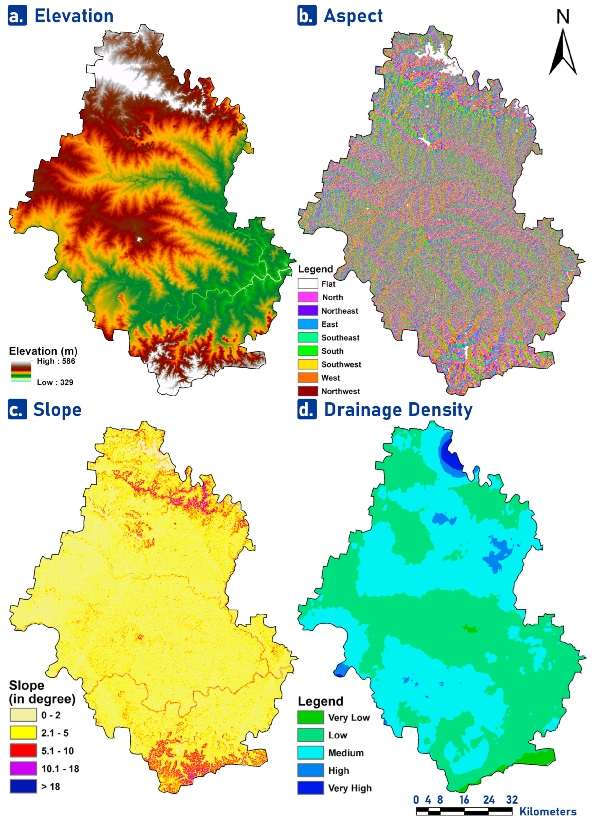
3.1.1. Elevation
3.1.2. Aspect
3.1.3. Slope
3.1.4. Drainage Density
3.1.5. Rainfall
3.1.6. Land Use Land Cover (LULC)
3.1.7. Lineaments Density
3.1.8. Lithology
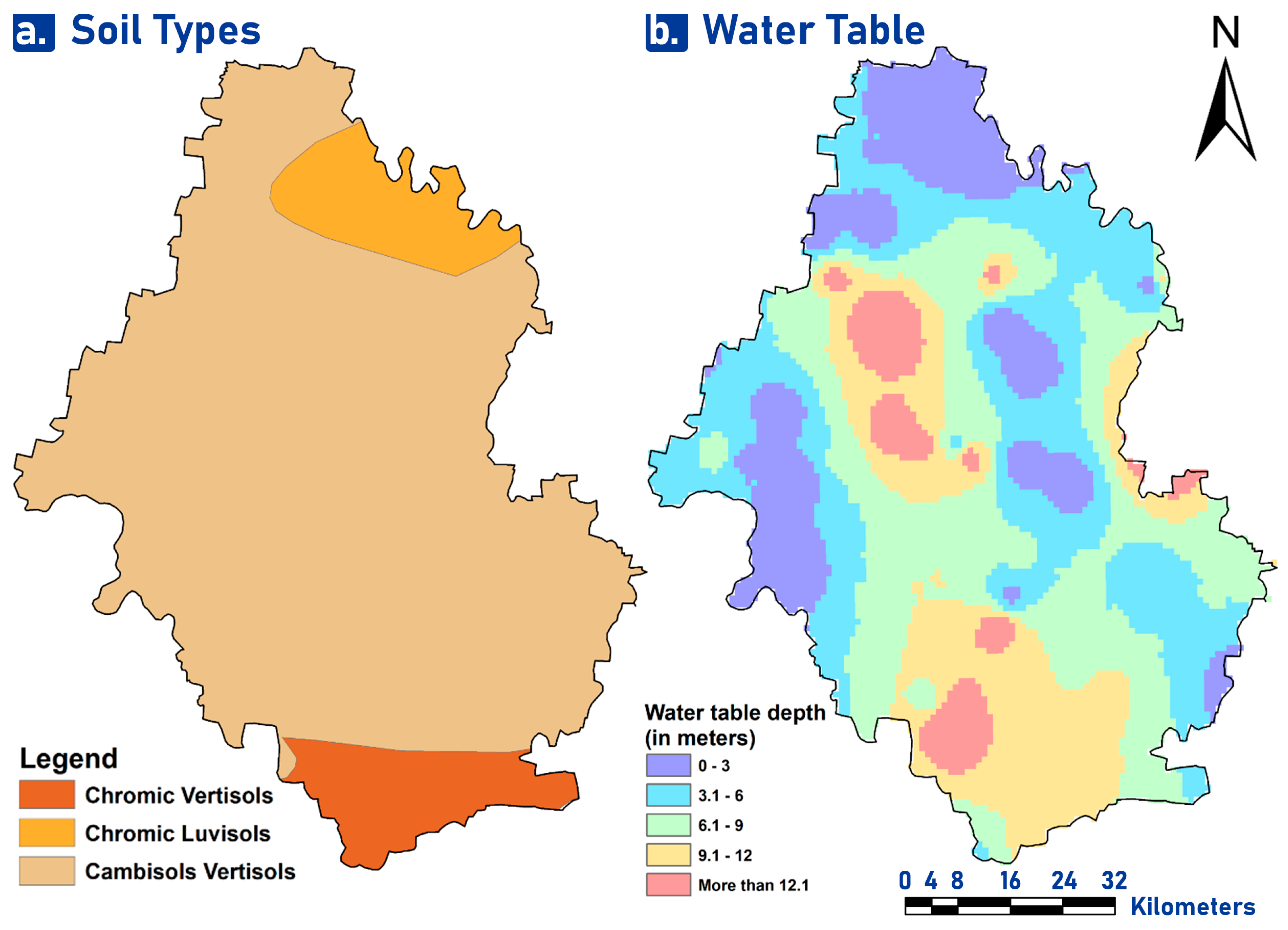
3.1.9. Soil Type
3.1.10. Water Table
3.2. Optimization of Machine Learning Algorithms
3.2.1. ANN-MLP
3.2.2. Random Forest (RF)
3.2.3. SMOreg
3.2.4. M5P
3.3. Validation Method
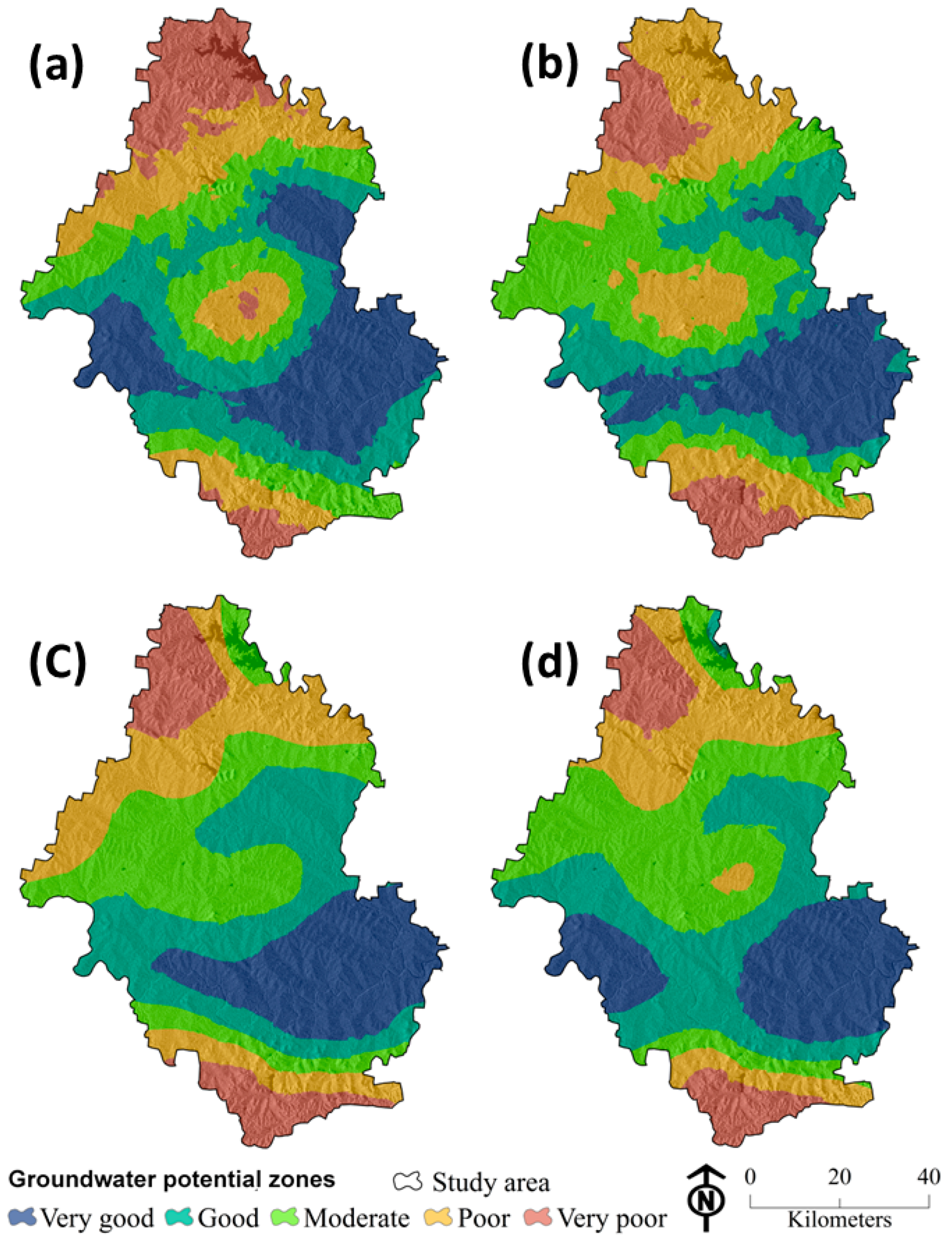
4. Results
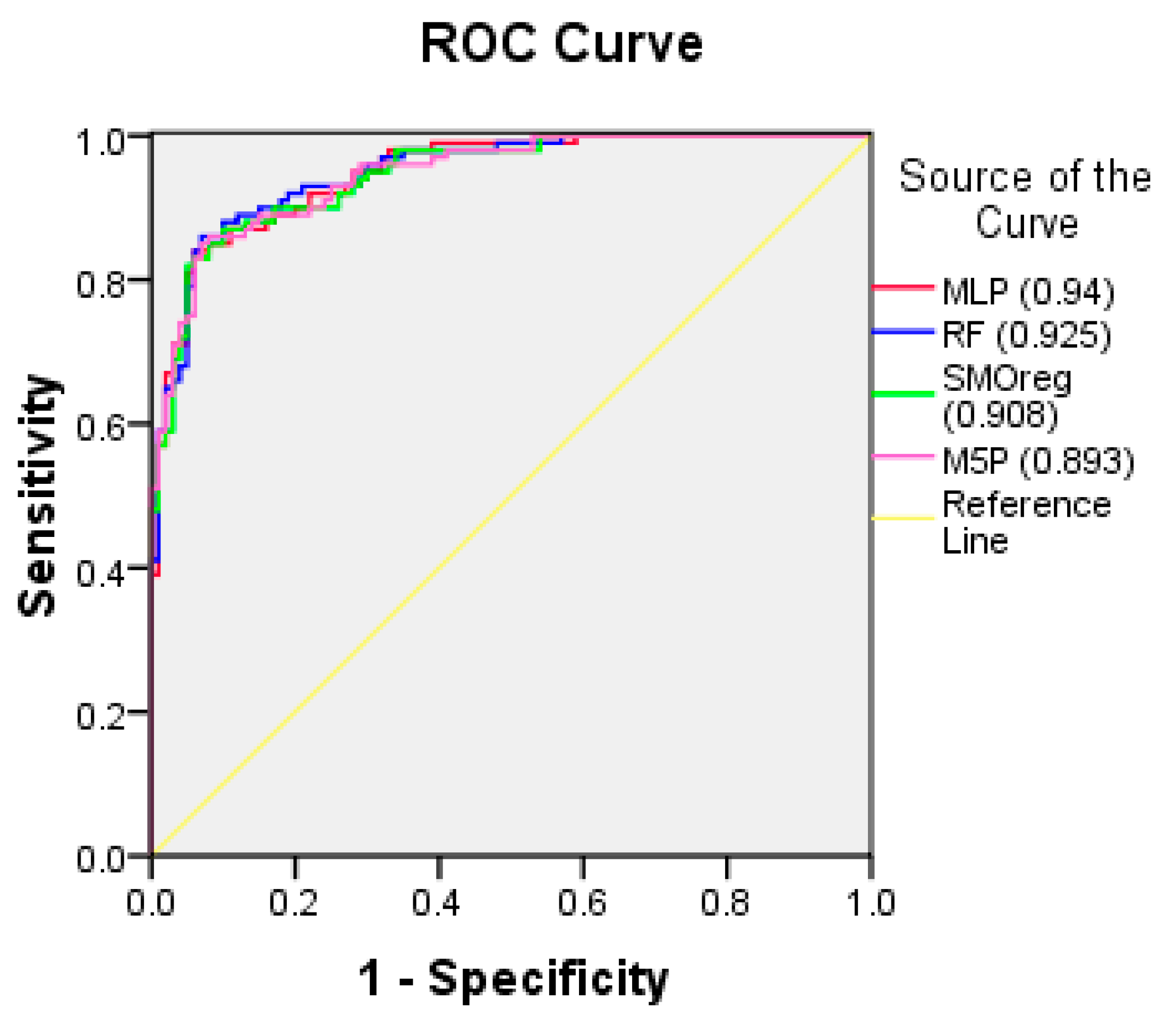
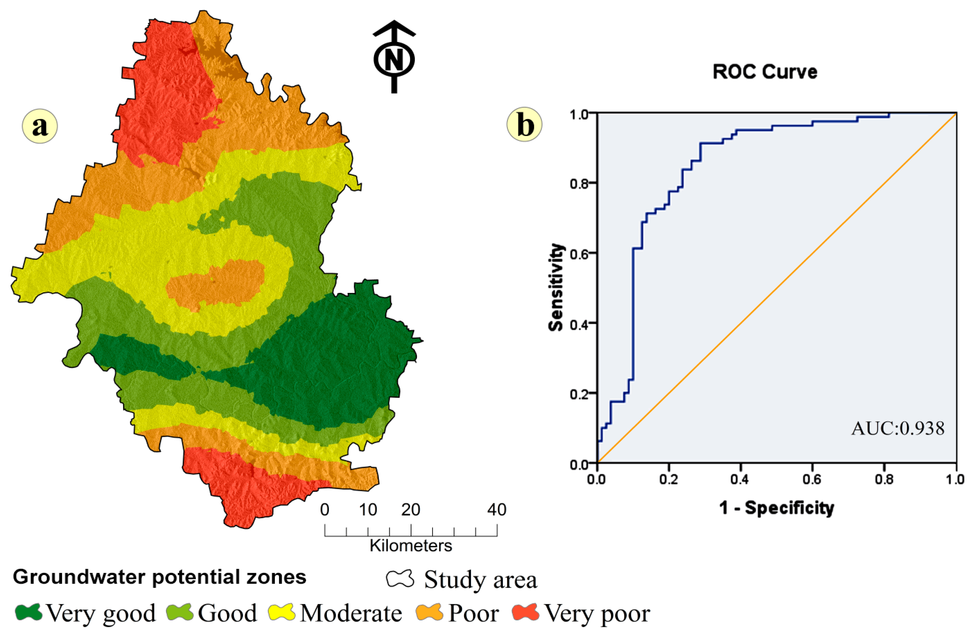
Validation of Groundwater Potential Maps Using ROC Curve and Field Data
5. Discussion
6. Conclusions
Author Contributions
Funding
Data Availability Statement
Acknowledgments
Conflicts of Interest
References
- Choudhari, P.P.; Nigam, G.K.; Singh, S.K.; Thakur, S. Morphometric based prioritization of watershed for groundwater potential of Mula river basin, Maharashtra, India. Geol. Ecol. Landsc. 2018, 2, 256–267. [Google Scholar] [CrossRef] [Green Version]
- He, L.; Shao, F.; Ren, L. Sustainability appraisal of desired contaminated groundwater remediation strategies: An information-entropy-based stochastic multi-criteria preference model. Environ. Dev. Sustain. 2020, 23, 1759–1779. [Google Scholar] [CrossRef]
- Macklin, M.G.; Lewin, J. The rivers of civilization. Quat. Sci. Rev. 2015, 114, 228–244. [Google Scholar] [CrossRef]
- Sachdeva, S.; Kumar, B. A novel ensemble model of automatic multilayer perceptron, random forest, and ZeroR for groundwater potential mapping. Environ. Monit. Assess. 2021, 193, 722. [Google Scholar] [CrossRef] [PubMed]
- Masroor, M.; Rehman, S.; Sajjad, H.; Rahaman, H.; Sahana, M.; Ahmed, R.; Singh, R. Assessing the impact of drought conditions on groundwater potential in Godavari Middle Sub-Basin, India using analytical hierarchy process and random forest machine learning algorithm. Groundw. Sustain. Dev. 2021, 13, 100554. [Google Scholar] [CrossRef]
- Mourot, F.M.; Westerhoff, R.S.; White, P.A.; Cameron, S.G. Climate change and New Zealand’s groundwater resources: A methodology to support adaptation. J. Hydrol. Reg. Stud. 2022, 40, 101053. [Google Scholar] [CrossRef]
- Velasco, E.M.; Gurdak, J.J.; Dickinson, J.E.; Ferré, T.; Corona, C.R. Interannual to multidecadal climate forcings on groundwater resources of the U.S. West Coast. J. Hydrol. Reg. Stud. 2017, 11, 250–265. [Google Scholar] [CrossRef] [Green Version]
- Taylor, R.G.; Scanlon, B.; Döll, P.; Rodell, M.; Van Beek, R.; Wada, Y.; Longuevergne, L.; Leblanc, M.; Famiglietti, J.S.; Edmunds, M.; et al. Ground water and climate change. Nat. Clim. Chang. 2013, 3, 322–329. [Google Scholar] [CrossRef] [Green Version]
- Bozorg-Haddad, O.; Zolghadr-Asli, B.; Sarzaeim, P.; Aboutalebi, M.; Chu, X.; Loáiciga, H.A. Evaluation of water shortage crisis in the Middle East and possible remedies. J. Water Supply Res. Technol. 2019, 69, 85–98. [Google Scholar] [CrossRef]
- Feng, P.; Wang, B.; Liu, D.L.; Ji, F.; Niu, X.; Ruan, H.; Shi, L.; Yu, Q. Machine learning-based integration of large-scale climate drivers can improve the forecast of seasonal rainfall probability in Australia. Environ. Res. Lett. 2020, 15, 084051. [Google Scholar] [CrossRef]
- Khosravi, K.; Khozani, Z.S.; Cooper, J.R. Predicting stable gravel-bed river hydraulic geometry: A test of novel, advanced, hybrid data mining algorithms. Environ. Model. Softw. 2021, 144, 105165. [Google Scholar] [CrossRef]
- Ganapuram, S.; Kumar, G.V.; Krishna, I.M.; Kahya, E.; Demirel, M.C. Mapping of groundwater potential zones in the Musi basin using remote sensing data and GIS. Adv. Eng. Softw. 2009, 40, 506–518. [Google Scholar] [CrossRef]
- Arulbalaji, P.; Padmalal, D.; Sreelash, K. GIS and AHP Techniques Based Delineation of Groundwater Potential Zones: A case study from Southern Western Ghats, India. Sci. Rep. 2019, 9, 2082. [Google Scholar] [CrossRef] [PubMed] [Green Version]
- Rahaman, H.; Sajjad, H.; Roshani; Masroor, M.; Bhuyan, N.; Rehman, S. Delineating groundwater potential zones using geospatial techniques and fuzzy analytical hierarchy process (FAHP) ensemble in the data-scarce region: Evidence from the lower Thoubal river watershed of Manipur, India. Arab. J. Geosci. 2022, 15, 677. [Google Scholar] [CrossRef]
- Rajasekhar, M.; Raju, G.S.; Sreenivasulu, Y.; Raju, R.S. Delineation of groundwater potential zones in semi-arid region of Jilledubanderu river basin, Anantapur District, Andhra Pradesh, India using fuzzy logic, AHP and integrated fuzzy-AHP approaches. Hydroresearch 2019, 2, 97–108. [Google Scholar] [CrossRef]
- Elvis, B.W.W.; Arsène, M.; Théophile, N.M.; Bruno, K.M.E.; Olivier, O.A. Integration of shannon entropy (SE), frequency ratio (FR) and analytical hierarchy process (AHP) in GIS for suitable groundwater potential zones targeting in the Yoyo river basin, Méiganga area, Adamawa Cameroon. J. Hydrol. Reg. Stud. 2022, 39, 100997. [Google Scholar] [CrossRef]
- Pourghasemi, H.R.; Beheshtirad, M. Assessment of a data-driven evidential belief function model and GIS for groundwater potential mapping in the Koohrang Watershed, Iran. Geocarto Int. 2014, 30, 662–685. [Google Scholar] [CrossRef]
- Golkarian, A.; Rahmati, O. Use of a maximum entropy model to identify the key factors that influence groundwater availability on the Gonabad Plain, Iran. Environ. Earth Sci. 2018, 77, 369. [Google Scholar] [CrossRef]
- Tahmassebipoor, N.; Rahmati, O.; Noormohamadi, F.; Lee, S. Spatial analysis of groundwater potential using weights-of-evidence and evidential belief function models and remote sensing. Arab. J. Geosci. 2015, 9, 79. [Google Scholar] [CrossRef]
- Park, S.; Hamm, S.-Y.; Jeon, H.-T.; Kim, J. Evaluation of Logistic Regression and Multivariate Adaptive Regression Spline Models for Groundwater Potential Mapping Using R and GIS. Sustainability 2017, 9, 1157. [Google Scholar] [CrossRef]
- Bloomfield, J.; Lewis, M.; Newell, A.; Loveless, S.; Stuart, M. Characterising variations in the salinity of deep groundwater systems: A case study from Great Britain (GB). J. Hydrol. Reg. Stud. 2020, 28, 100684. [Google Scholar] [CrossRef]
- Hakim, W.L.; Nur, A.S.; Rezaie, F.; Panahi, M.; Lee, C.-W.; Lee, S. Convolutional neural network and long short-term memory algorithms for groundwater potential mapping in Anseong, South Korea. J. Hydrol. Reg. Stud. 2022, 39, 100990. [Google Scholar] [CrossRef]
- Arabameri, A.; Pal, S.C.; Rezaie, F.; Nalivan, O.A.; Chowdhuri, I.; Saha, A.; Lee, S.; Moayedi, H. Modeling groundwater potential using novel GIS-based machine-learning ensemble techniques. J. Hydrol. Reg. Stud. 2021, 36, 100848. [Google Scholar] [CrossRef]
- Pal, S.; Sarda, R. Modelling water richness in riparian flood plain wetland using bivariate statistics and machine learning algo-rithms and figuring out the role of damming. Geocarto Int. 2022, 37, 5585–5608. [Google Scholar] [CrossRef]
- Dai, F.; Lee, C.; Zhang, X. GIS-based geo-environmental evaluation for urban land-use planning: A case study. Eng. Geol. 2001, 61, 257–271. [Google Scholar] [CrossRef]
- Chen, W.; Li, H.; Hou, E.; Wang, S.; Wang, G.; Panahi, M.; Li, T.; Peng, T.; Guo, C.; Niu, C.; et al. GIS-based groundwater potential analysis using novel ensemble weights-of-evidence with logistic regression and functional tree models. Sci. Total Environ. 2018, 634, 853–867. [Google Scholar] [CrossRef] [Green Version]
- Kordestani, M.D.; Naghibi, S.A.; Hashemi, H.; Ahmadi, K.; Kalantar, B.; Pradhan, B. Groundwater potential mapping using a novel data-mining ensemble model. Hydrogeol. J. 2018, 27, 211–224. [Google Scholar] [CrossRef] [Green Version]
- Nguyen, P.T.; Ha, D.H.; Jaafari, A.; Nguyen, H.D.; Van Phong, T.; Al-Ansari, N.; Prakash, I.; Van Le, H.; Pham, B.T. Groundwater Potential Mapping Combining Artificial Neural Network and Real AdaBoost Ensemble Technique: The DakNong Province Case-study, Vietnam. Int. J. Environ. Res. Public Health 2020, 17, 2473. [Google Scholar] [CrossRef] [Green Version]
- Pham, B.T.; Jaafari, A.; Prakash, I.; Singh, S.K.; Quoc, N.K.; Bui, D.T. Hybrid computational intelligence models for groundwater potential mapping. Catena 2019, 182, 104101. [Google Scholar] [CrossRef]
- Naghibi, S.A.; Ahmadi, K.; Daneshi, A. Application of Support Vector Machine, Random Forest, and Genetic Algorithm Optimized Random Forest Models in Groundwater Potential Mapping. Water Resour. Manag. 2017, 31, 2761–2775. [Google Scholar] [CrossRef]
- Choubin, B.; Rahmati, O.; Soleimani, F.; Alilou, H.; Moradi, E.; Alamdari, N. Regional Groundwater Potential Analysis Using Classification and Regression Trees. In Spatial Modeling in GIS and R for Earth and Environmental Sciences; Elsevier: Amsterdam, The Netherlands, 2019; pp. 485–498. [Google Scholar] [CrossRef]
- Sun, X.; Zhou, Y.; Yuan, L.; Li, X.; Shao, H.; Lu, X. Integrated decision-making model for groundwater potential evaluation in mining areas using the cusp catastrophe model and principal component analysis. J. Hydrol. Reg. Stud. 2021, 37, 100891. [Google Scholar] [CrossRef]
- Panahi, M.; Sadhasivam, N.; Pourghasemi, H.R.; Rezaie, F.; Lee, S. Spatial prediction of groundwater potential mapping based on convolutional neural network (CNN) and support vector regression (SVR). J. Hydrol. 2020, 588, 125033. [Google Scholar] [CrossRef]
- Al-Fugara, A.; Ahmadlou, M.; Shatnawi, R.; AlAyyash, S.; Al-Adamat, R.; Al-Shabeeb, A.A.-R.; Soni, S. Novel hybrid models combining meta-heuristic algorithms with support vector regression (SVR) for groundwater potential mapping. Geocarto Int. 2020, 37, 2627–2646. [Google Scholar] [CrossRef]
- Zabihi, M.; Pourghasemi, H.R.; Pourtaghi, Z.S.; Behzadfar, M. GIS-based multivariate adaptive regression spline and random forest models for groundwater potential mapping in Iran. Environ. Earth Sci. 2016, 75, 1097. [Google Scholar] [CrossRef]
- Moghaddam, D.D.; Rahmati, O.; Panahi, M.; Tiefenbacher, J.; Darabi, H.; Haghizadeh, A.; Haghighi, A.T.; Nalivan, O.A.; Tien Bui, D. The effect of sample size on different machine learning models for groundwater potential mapping in mountain bedrock aquifers. CATENA 2020, 187, 104421. [Google Scholar] [CrossRef]
- Adeyeye, O.; Ikpokonte, E.; Arabi, S. GIS-based groundwater potential mapping within Dengi area, North Central Nigeria. Egypt. J. Remote. Sens. Space Sci. 2018, 22, 175–181. [Google Scholar] [CrossRef]
- Arabameri, A.; Arora, A.; Pal, S.C.; Mitra, S.; Saha, A.; Nalivan, O.A.; Panahi, S.; Moayedi, H. K-Fold and State-of-the-Art Metaheuristic Machine Learning Approaches for Groundwater Potential Modelling. Water Resour. Manag. 2021, 35, 1837–1869. [Google Scholar] [CrossRef]
- Chen, W.; Zhao, X.; Tsangaratos, P.; Shahabi, H.; Ilia, I.; Xue, W.; Wang, X.; Bin Ahmad, B. Evaluating the usage of tree-based ensemble methods in groundwater spring potential mapping. J. Hydrol. 2020, 583, 124602. [Google Scholar] [CrossRef]
- Chandramouli, C. Census of India: Primary Census Abstract; Office of the Registrar General & Census Commissioner, India: New Delhi, India, 2013.
- Masroor, M.; Rehman, S.; Avtar, R.; Sahana, M.; Ahmed, R.; Sajjad, H. Exploring climate variability and its impact on drought occurrence: Evidence from Godavari Middle sub-basin, India. Weather Clim. Extrem. 2020, 30, 100277. [Google Scholar] [CrossRef]
- Tarate, S.B.; Kumar, P. Characterization and trend detection of meteorological drought for a semi-arid area of Parbhani district of Indian state of Maharashtra. Mausam 2021, 72, 583–596. [Google Scholar] [CrossRef]
- Dakhore, K.K.; Rathod, A.S.; Kadam, D.R.; Shinde, G.U.; Kadam, Y.E.; Ghosh, K. Prediction of Kharif cotton yield over Parbhani, Maharashtra: Combination of extended range forecast and DSSAT-CROPGRO-Cotton model. Mausam 2021, 72, 635–644. [Google Scholar] [CrossRef]
- Dakhore, K.K.; Kadam, Y.E.; Vijaya, K.P. Study the rainfall variability and impact of El Nino episode on rainfall and crop productivity at Parbhani. Mausam 2020, 71, 285–290. [Google Scholar] [CrossRef]
- Mukherjee, I.; Singh, U.K. Delineation of groundwater potential zones in a drought-prone semi-arid region of east India using GIS and analytical hierarchical process techniques. Catena 2020, 194, 104681. [Google Scholar] [CrossRef]
- Ahmed, R.; Sajjad, H.; Husain, I. Morphometric Parameters-Based Prioritization of Sub-watersheds Using Fuzzy Analytical Hierarchy Process: A Case Study of Lower Barpani Watershed, India. Nat. Resour. Res. 2017, 27, 67–75. [Google Scholar] [CrossRef]
- Shao, Z.; Huq, E.; Cai, B.; Altan, O.; Li, Y. Integrated remote sensing and GIS approach using Fuzzy-AHP to delineate and identify groundwater potential zones in semi-arid Shanxi Province, China. Environ. Model. Softw. 2020, 134, 104868. [Google Scholar] [CrossRef]
- Doke, A.B.; Zolekar, R.B.; Patel, H.; Das, S. Geospatial mapping of groundwater potential zones using multi-criteria decision-making AHP approach in a hardrock basaltic terrain in India. Ecol. Indic. 2021, 127, 107685. [Google Scholar] [CrossRef]
- Akhtar, N.; Syakir, M.I.; Anees, M.T.; Qadir, A.; Yusuff, M.S. Characteristics and Assessment of Groundwater. In Groundwater Management and Resources; IntechOpen: London, UK, 2021. [Google Scholar] [CrossRef]
- Chitsazan, M.; Akhtari, Y. A GIS-based DRASTIC Model for Assessing Aquifer Vulnerability in Kherran Plain, Khuzestan, Iran. Water Resour. Manag. 2008, 23, 1137–1155. [Google Scholar] [CrossRef]
- Madrucci, V.; Taioli, F.; de Araújo, C.C. Groundwater favorability map using GIS multicriteria data analysis on crystalline terrain, São Paulo State, Brazil. J. Hydrol. 2008, 357, 153–173. [Google Scholar] [CrossRef]
- Pradhan, R.M.; Guru, B.; Pradhan, B.; Biswal, T.K. Integrated multi-criteria analysis for groundwater potential mapping in Precambrian hard rock terranes (North Gujarat), India. Hydrol. Sci. J. 2021, 66, 961–978. [Google Scholar] [CrossRef]
- Alqadhi, S.; Mallick, J.; Talukdar, S.; Bindajam, A.A.; Saha, T.K.; Ahmed, M.; Khan, R.A. Combining logistic regression-based hybrid optimized machine learning algorithms with sensitivity analysis to achieve robust landslide susceptibility mapping. Geocarto Int. 2022, 1–26. [Google Scholar] [CrossRef]
- Lee, J.; Kim, C.-G.; Lee, J.E.; Kim, N.W.; Kim, H. Application of Artificial Neural Networks to Rainfall Forecasting in the Geum River Basin, Korea. Water 2018, 10, 1448. [Google Scholar] [CrossRef] [Green Version]
- Razavi-Termeh, S.V.; Sadeghi-Niaraki, A.; Choi, S.-M. Groundwater Potential Mapping Using an Integrated Ensemble of Three Bivariate Statistical Models with Random Forest and Logistic Model Tree Models. Water 2019, 11, 1596. [Google Scholar] [CrossRef] [Green Version]
- Masroor, M.; Sajjad, H.; Rehman, S.; Singh, R.; Rahaman, H.; Sahana, M.; Ahmed, R.; Avtar, R. Analysing the relationship between drought and soil erosion using vegetation health index and RUSLE models in Godavari middle sub-basin, India. Geosci. Front. 2021, 13, 101312. [Google Scholar] [CrossRef]
- Alhatali, A.; Soosaimanickam, A. A Comparative Study of the Efficient Data Mining Algorithm to Find the Most Influenced Fac-tor on Price Variation in Oman Fish Markets. Sak. Univ. J. Comput. Inf. Sci. 2018, 1, 1–16. [Google Scholar]
- Cortes, C.; Vapnik, V. Support-vector networks. Mach. Learn. 1995, 20, 273–297. [Google Scholar] [CrossRef]
- Zhang, L.; Traore, S.; Ge, J.; Li, Y.; Wang, S.; Zhu, G.; Cui, Y.; Fipps, G. Using boosted tree regression and artificial neural networks to forecast upland rice yield under climate change in Sahel. Comput. Electron. Agric. 2019, 166, 105031. [Google Scholar] [CrossRef]
- Platt, J. Sequential Minimal Optimization: A Fast Algorithm for Training Support Vector Machines (Issue MSR-TR-98-14). 1998. Available online: https://www.microsoft.com/en-us/research/publication/sequential-minimal-optimization-a-fast-algorithm-for-training-support-vector-machines/ (accessed on 16 January 2023).
- Myers, S.A.; Leskovec, J. The bursty dynamics of the Twitter information network. In Proceedings of the 23rd International Conference on World Wide Web—WWW ’14, Seoul, Republic of Korea, 7–11 April 2014; pp. 913–924. [Google Scholar] [CrossRef] [Green Version]
- Abdelkarim, A.; Al-Alola, S.S.; Alogayell, H.M.; Mohamed, S.A.; Alkadi, I.I.; Youssef, I.Y. Mapping of GIS-Flood Hazard Using the Geomorphometric-Hazard Model: Case Study of the Al-Shamal Train Pathway in the City of Qurayyat, Kingdom of Saudi Arabia. Geosciences 2020, 10, 333. [Google Scholar] [CrossRef]
- Granata, F.; Saroli, M.; De Marinis, G.; Gargano, R. Machine Learning Models for Spring Discharge Forecasting. Geofluids 2018, 2018, 1–13. [Google Scholar] [CrossRef]
- Masroor, M.; Razavi-Termeh, S.V.; Rahaman, H.; Choudhari, P.; Kulimushi, L.C.; Sajjad, H. Adaptive neuro fuzzy inference system (ANFIS) machine learning algorithm for assessing environmental and socio-economic vulnerability to drought: A study in Godavari middle sub-basin, India. Stoch. Environ. Res. Risk Assess. 2022, 37, 233–259. [Google Scholar] [CrossRef]
- Kulimushi, L.C.; Bashagaluke, J.B.; Prasad, P.; Heri-Kazi, A.B.; Kushwaha, N.L.; Masroor, M.; Mohammed, S. Soil erosion sus-ceptibility mapping using ensemble machine learning models: A case study of upper Congo river sub-basin. Catena 2023, 222, 106858. [Google Scholar] [CrossRef]
- Das, J.; Mandal, T.; Rahman, A.T.M.S.; Saha, P. Spatio-temporal characterization of rainfall in Bangladesh: An innovative trend and discrete wavelet transformation approaches. Theor. Appl. Clim. 2021, 143, 1557–1579. [Google Scholar] [CrossRef]
- Saha, T.K.; Pal, S. Exploring physical wetland vulnerability of Atreyee river basin in India and Bangladesh using logistic regression and fuzzy logic approaches. Ecol. Indic. 2018, 98, 251–265. [Google Scholar] [CrossRef]
- Djurovic, N.; Domazet, M.; Stričević, R.; Pocuca, V.; Spalevic, V.; Pivic, R.; Gregoric, E.; Domazet, U. Comparison of Groundwater Level Models Based on Artificial Neural Networks and ANFIS. Sci. World J. 2015, 2015, 1–13. [Google Scholar] [CrossRef] [Green Version]
- Cai, H.; Shi, H.; Liu, S.; Babovic, V. Impacts of regional characteristics on improving the accuracy of groundwater level prediction using machine learning: The case of central eastern continental United States. J. Hydrol. Reg. Stud. 2021, 37, 100930. [Google Scholar] [CrossRef]
- Shadkani, S.; Abbaspour, A.; Samadianfard, S.; Hashemi, S.; Mosavi, A.; Band, S.S. Comparative study of multilayer perceptron-stochastic gradient descent and gradient boosted trees for predicting daily suspended sediment load: The case study of the Mississippi River, U.S. Int. J. Sediment Res. 2020, 36, 512–523. [Google Scholar] [CrossRef]
- Allam, A.; Moussa, R.; Najem, W.; Bocquillon, C. Hydrological cycle, Mediterranean basins hydrology. In Water Resources in the Mediterranean Region; Elsevier: Amsterdam, The Netherlands, 2020; pp. 1–21. [Google Scholar] [CrossRef]
- Al-Djazouli, M.O.; Elmorabiti, K.; Rahimi, A.; Amellah, O.; Fadil, O.A.M. Delineating of groundwater potential zones based on remote sensing, GIS and analytical hierarchical process: A case of Waddai, eastern Chad. Geo J. 2020, 86, 1881–1894. [Google Scholar] [CrossRef]


| S. No | Factors | Data Type | Source of Data | Data Details | Time Period |
|---|---|---|---|---|---|
| 1 | Aspect | Raster layer | SRTM DEM, version 3.0, (USGS) | 30 m spatial resolution | 2018 |
| 2 | Elevation | Raster layer | SRTM DEM, version 3.0, (USGS) | 30 m spatial resolution | 2018 |
| 3 | Slope | Raster layer | SRTM DEM, version 3.0, (USGS) | 30 m spatial resolution | 2018 |
| 4 | Lineament density | Vector data | Bhuvan thematic services of National Remote Sensing Centre | 1:50,000 | 2011 |
| 5 | Drainage density | Raster layer | SRTM DEM, version 3.0, (USGS) | 30 m spatial resolution | 2018 |
| 6 | Lithology | Vector data | Bhuvan thematic services of National Remote Sensing Centre | 1:50,000 | 2005–2006 |
| 7 | Land use land cover | Raster layer | LANDSAT 8 OLI | 30 m spatial resolution | December (2018) |
| 8 | Rainfall | Vector data | Indian Metrological Department (IMD) | Annual average rainfall in mm | 2018 |
| 9 | Water table | Vector data | Central Groundwater Board (CGWB) | water table depth in meters | 2018 |
| 10 | Soil type | Vector data | Food and Agriculture Organization | 1:5,000,000 | 2017 |
| Performance Indicators | Applied Models | |||
|---|---|---|---|---|
| ANN-MLP | RF | SMOReg | M5P | |
| Mean absolute error (MAE) | 0.0962 | 0.1309 | 0.223 | 0.347 |
| Root mean squared error (RMSE) | 0.1104 | 0.1594 | 0.2831 | 0.3915 |
| Relative absolute error (RAE) | 19.83% | 26.18% | 29.33% | 30.08% |
| Root relative squared error (RRSE) | 28.07% | 31.07% | 33.43% | 37.68% |
| Groundwater Potential Zone | ANN-MLP | RF | SMOReg | M5P | ||||
|---|---|---|---|---|---|---|---|---|
| Pixels | % of Area | Pixels | % of Area | Pixels | % of Area | Pixels | % of Area | |
| Very good | 1,813,819 | 24.81 | 1,403,665 | 19.20 | 1,431,676 | 19.58 | 1,513,213 | 20.69 |
| Good | 1,735,058 | 23.73 | 1,477,614 | 20.21 | 1,733,015 | 23.70 | 1,836,131 | 25.11 |
| Moderate | 1,505,579 | 20.59 | 1,909,177 | 26.11 | 1,877,586 | 25.68 | 2,085,097 | 28.52 |
| Poor | 1,322,992 | 18.09 | 1,798,071 | 24.59 | 1,457,208 | 19.93 | 1,210,145 | 16.55 |
| Very poor | 934,827 | 12.78 | 723,748 | 9.90 | 812,790 | 11.12 | 667,689 | 9.13 |
| ML Models | Area (AUC) | |
|---|---|---|
| Training Datasets | Testing Datasets | |
| ANN-MLP | 0.91 | 0.94 |
| RF | 0.902 | 0.925 |
| SMOReg | 0.893 | 0.908 |
| M5P | 0.881 | 0.893 |
| Groundwater Potential Zones | Pixels | % of Area |
|---|---|---|
| Very good | 1,323,194 | 18.10 |
| good | 1,587,893 | 21.72 |
| Moderate | 1,796,215 | 24.56 |
| poor | 1,614,995 | 22.09 |
| Very poor | 989,978 | 13.54 |
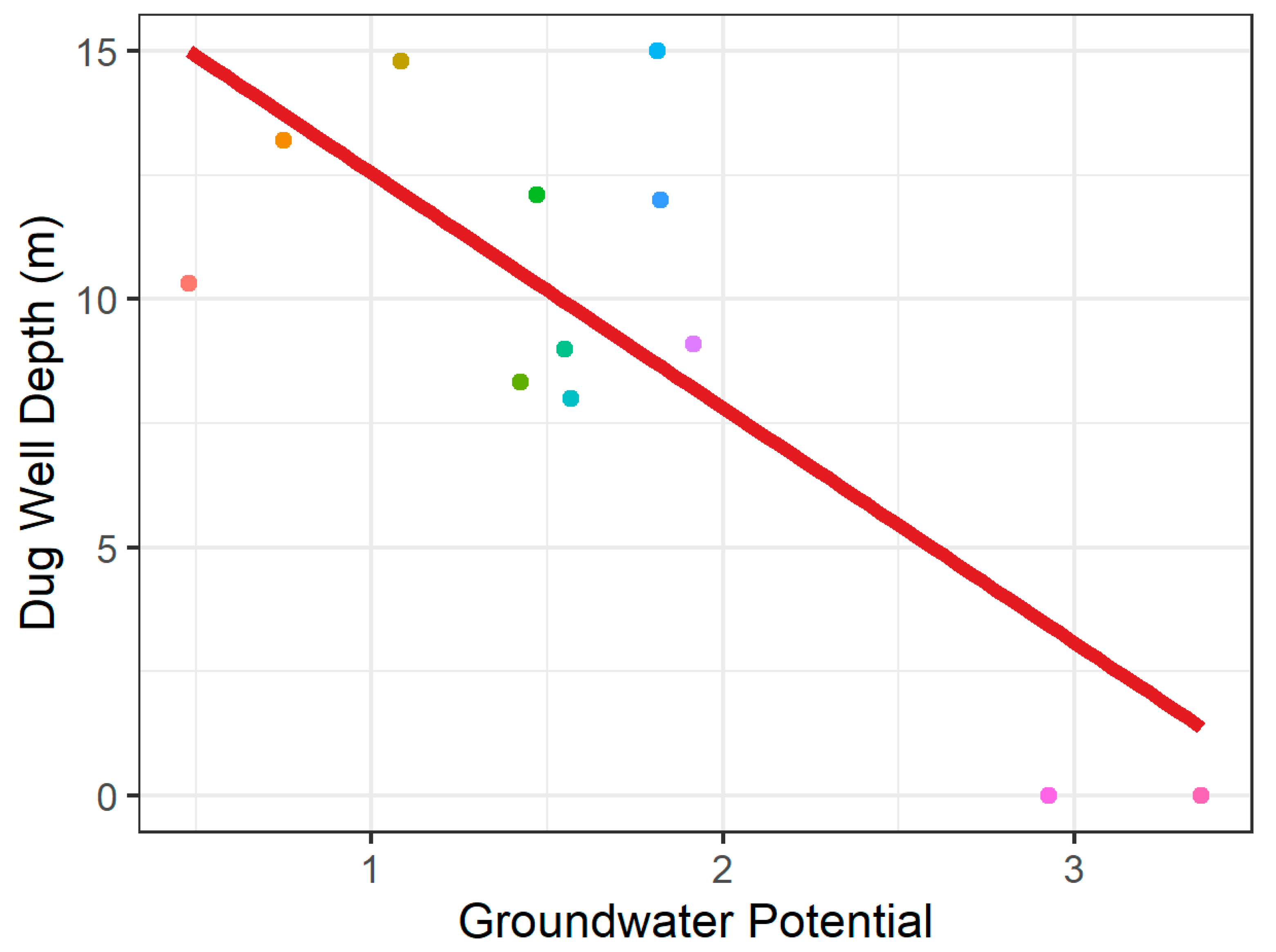
| S.No. | Block Name | Lat | Lon | Site Type | Depth of Dug Well (m) |
|---|---|---|---|---|---|
| 1 | Manwat | 19.3438 | 76.5616 | Dug well | 15 |
| 2 | Parbhani | 19.4263 | 76.7658 | Dug well | 14.8 |
| 3 | Palam | 18.9833 | 76.8666 | Dug well | 13.2 |
| 4 | Jintur | 19.4855 | 76.7225 | Dug well | 12.1 |
| 5 | Pathri | 19.30 | 76.30 | Dug well | 12 |
| 6 | Palam | 19.0194 | 76.8347 | Dug well | 10.32 |
| 7 | Jintur | 19.5447 | 76.9588 | Dug well | 9.1 |
| 8 | Gangakhed | 18.9655 | 76.7311 | Dug well | 9 |
| 9 | Parbhani | 19.2661 | 76.8225 | Dug well | 8.32 |
| 10 | Parbhani | 19.3875 | 76.6875 | Dug Well | 8 |
| 11 | Jintur | 19.6222 | 76.5391 | Dug Well | 0 |
| 12 | Jintur | 19.718 | 76.6572 | Dug Well | 0 |
Disclaimer/Publisher’s Note: The statements, opinions and data contained in all publications are solely those of the individual author(s) and contributor(s) and not of MDPI and/or the editor(s). MDPI and/or the editor(s) disclaim responsibility for any injury to people or property resulting from any ideas, methods, instructions or products referred to in the content. |
© 2023 by the authors. Licensee MDPI, Basel, Switzerland. This article is an open access article distributed under the terms and conditions of the Creative Commons Attribution (CC BY) license (https://creativecommons.org/licenses/by/4.0/).
Share and Cite
Masroor, M.; Sajjad, H.; Kumar, P.; Saha, T.K.; Rahaman, M.H.; Choudhari, P.; Kulimushi, L.C.; Pal, S.; Saito, O. Novel Ensemble Machine Learning Modeling Approach for Groundwater Potential Mapping in Parbhani District of Maharashtra, India. Water 2023, 15, 419. https://doi.org/10.3390/w15030419
Masroor M, Sajjad H, Kumar P, Saha TK, Rahaman MH, Choudhari P, Kulimushi LC, Pal S, Saito O. Novel Ensemble Machine Learning Modeling Approach for Groundwater Potential Mapping in Parbhani District of Maharashtra, India. Water. 2023; 15(3):419. https://doi.org/10.3390/w15030419
Chicago/Turabian StyleMasroor, Md, Haroon Sajjad, Pankaj Kumar, Tamal Kanti Saha, Md Hibjur Rahaman, Pandurang Choudhari, Luc Cimusa Kulimushi, Swades Pal, and Osamu Saito. 2023. "Novel Ensemble Machine Learning Modeling Approach for Groundwater Potential Mapping in Parbhani District of Maharashtra, India" Water 15, no. 3: 419. https://doi.org/10.3390/w15030419