
Propagation Modeling of Rainfall-Induced Landslides: A Case Study of the Shaziba Landslide in Enshi, China


1
Department of Civil Engineering, Shanghai University, Shanghai 200444, China
2
College of Environmental Science and Engineering, Donghua University, Shanghai 201620, China
*
Authors to whom correspondence should be addressed.
Water 2023, 15(3), 424; https://doi.org/10.3390/w15030424
Submission received: 4 December 2022
/
Revised: 15 January 2023
/
Accepted: 17 January 2023
/
Published: 20 January 2023
(This article belongs to the Special Issue Rainfall-Induced Geological Disasters)
Abstract
:Geological disasters, especially landslides, frequently occur in Enshi County, Hubei Province, China. On 21 July 2020, a large-scale landslide occurred in Enshi due to continuous rainfall. The landslide mass blocked the Qingjiang River, formed a dammed lake and caused great damage to surrounding roads and village buildings. In this study, the geomechanical properties of the landslide mass were obtained through field surveys. A three-dimensional topography model of the slope was established using the particle flow code (PFC) and the numerical parameters of the model were calibrated. A 3D discrete element model (DEM) was used to simulate the propagation of Shaziba landslide, and the dynamic behavior of the landslide was divided into five stages. The simulation results show that the landslide movement lasted approximately 1000 s. The maximum average velocity of the landslide reached up to 7.5 m/s and the average runout distance was about 1000 m. The simulated morphology of the landslide deposits was in good agreement with the field data. In addition, the influence of effective modulus on the calculation results was analyzed. The results indicate that the propagation behavior of a landslide and the morphology of landslide deposits are closely related to the effective modulus in the contact model of the PFC3D.
1. Introduction
Landslides are one of the major geological hazards in China, seriously threatening the safety of people’s lives and property. Rainfall is considered as a major trigger of landslides. More than 90% of landslides were reported to be triggered by rainfall events [1,2]. In recent decades, rainfall-induced landslides have caused huge loss of life and property in China. For instance, the Sanxicun landslide occurring in Dujiangyan, Sichuan Province in 2015 caused 166 deaths [3]. In 2019, 52 people were killed in the Jichang landslide in Liupanshui City, Guizhou Province [4]. The Zhongbao landslide occurring in Liujing Village, Chongqing City in 2020 blocked the Yancang River and created a dammed lake, threatening the lives and property of 152 families [5]. In 2021, a massive landslide in Tiejiangwan, Hongya County, Sichuan Province, left three people missing and damaged five houses [6]. Based on the field investigation of the above-mentioned landslides, it was observed that most rainfall-induced landslides can travel a long runout distance with a relative high velocity, which is usually defined as a flow-like landslide in the literature [7,8]. Therefore, it is of great importance to analyze the propagation behavior of typical rainfall-induced landslides for disaster prediction and prevention.
At present, the study of the post-failure behavior of landslides is mainly focused on field investigation [9,10], theoretical analysis [11], physical experiments [12,13,14] and numerical simulation [15,16]. Field surveys are useful to collect reliable primary data and to visually identify the characteristics of slopes after failure. However, most studies are still in the qualitative stage and cannot observe the dynamic characteristics of landslides [17]. The theoretical analysis usually contains many simplifications and assumptions, while the actual landslide situation is often complex [18]. Physical models are limited by scaling effects, so it is difficult to reconstruct accurate 3D topography models [19]. Compared with the above-mentioned methods, numerical simulation has the advantage of low cost and high performance. It can deal with complex engineering problems by building mathematical models [20,21]. Numerical simulation methods include mesh-based methods and mesh-free methods [22]. The mesh-based methods for landslide analysis mainly include FEM, FDM and so on. For example, Ozbay and Cabalar [23] carried out a series of FEM modeling to analyze the stability of slopes and evaluate factors that caused the landslides. Moayedi et al. [24] conducted different FEM analyses to determine susceptibility to landslides and consider appropriate countermeasures. Maugeri et al. [25] presented an FDM model to simulate the seasonal creep in natural slopes and predict the viscous deformations of a landslide body. Bozzano et al. [26] used an FDM approach to investigate the role of local seismic amplification in the reactivation of a landslide. This research shows the obvious advantages of the mesh-based methods in slope stability analysis, deformation prediction, dynamic response analysis and slope-retaining structure design. However, mesh-based methods suffer from some numerical problems, such as mesh winding and deformation, when dealing with the extremely large deformations involved in flow-like landslide propagation. Compared with mesh-based methods, the mesh-free methods have apparent advantages in modeling large deformations of landslides. For instance, Mcdougall and Hungr [27] proposed a Lagrangian solution called DAN for the analysis of rapid landslide propagation across 3D terrain, in which the landslide mass was assumed to be an equivalent fluid. Dai et al. [7] presented a 3D SPH model to simulate the post-failure behavior of a flow-like landslide triggered by a strong earthquake. Sitar et al. [28] carried out dynamic DDA simulations of the Vaiont landslide to discuss the influence of the geometric discontinuity on the kinematic features of landslides. Huang and Zhu [29] developed a modified MPS model for the simulation of flow slides in municipal solid waste dumps. Mast et al. [30] presented an MPM model to predict the flow dynamics of landslides and calculate the interaction force with structures. Some other research works regarding landslide modeling based on mesh-free methods were presented in Dai et al. [31], Mao et al. [32], Wang et al. [33], Yang et al. [34] and Chen et al. [35]. Recently, the discrete element method (DEM) has been widely used to simulate the propagation of catastrophic landslides [36,37,38,39]. As a numerical software based on the DEM method, particle flow code (PFC) has been widely applied to simulate the propagation of flow-like landslides. For example, Zou et al. [37] analyzed the kinetic characteristics of the Jiweishan rockslide in China based on a PFC model. Wei et al. [18] presented a PFC-based model to investigate the kinetics feature of the Mabian landslide. Wu et al. [40] established a 2D PFC model to analyze the dynamic response characteristics and deformation evolution process of loess slopes under seismic loads. Ray et al. [41] applied the PFC method to model the rheological properties of a landslide debris in Uttarkashi, India. Therefore, the PFC model is suitable to simulate the propagation behavior of different types of landslides.
This study aims to explore the propagation behavior of the Shaziba landslide in Enshi County, Hubei Province, China and reveal the kinetic characteristics of the landslide. The authors conducted a systematic survey of topographic features, geological structures, rainfall history and deformation characteristics in the study area. Based on the collected survey data, a landslide model based on PFC3D was presented to reproduce the landslide motion process and study the kinematic characteristics and accumulation morphology. The results of this work can provide a scientific basis for the study of this type of landslide in the Enshi area and contribute to disaster prevention and mitigation.
2. Study Areas
2.1. Overview of the Landslide Area
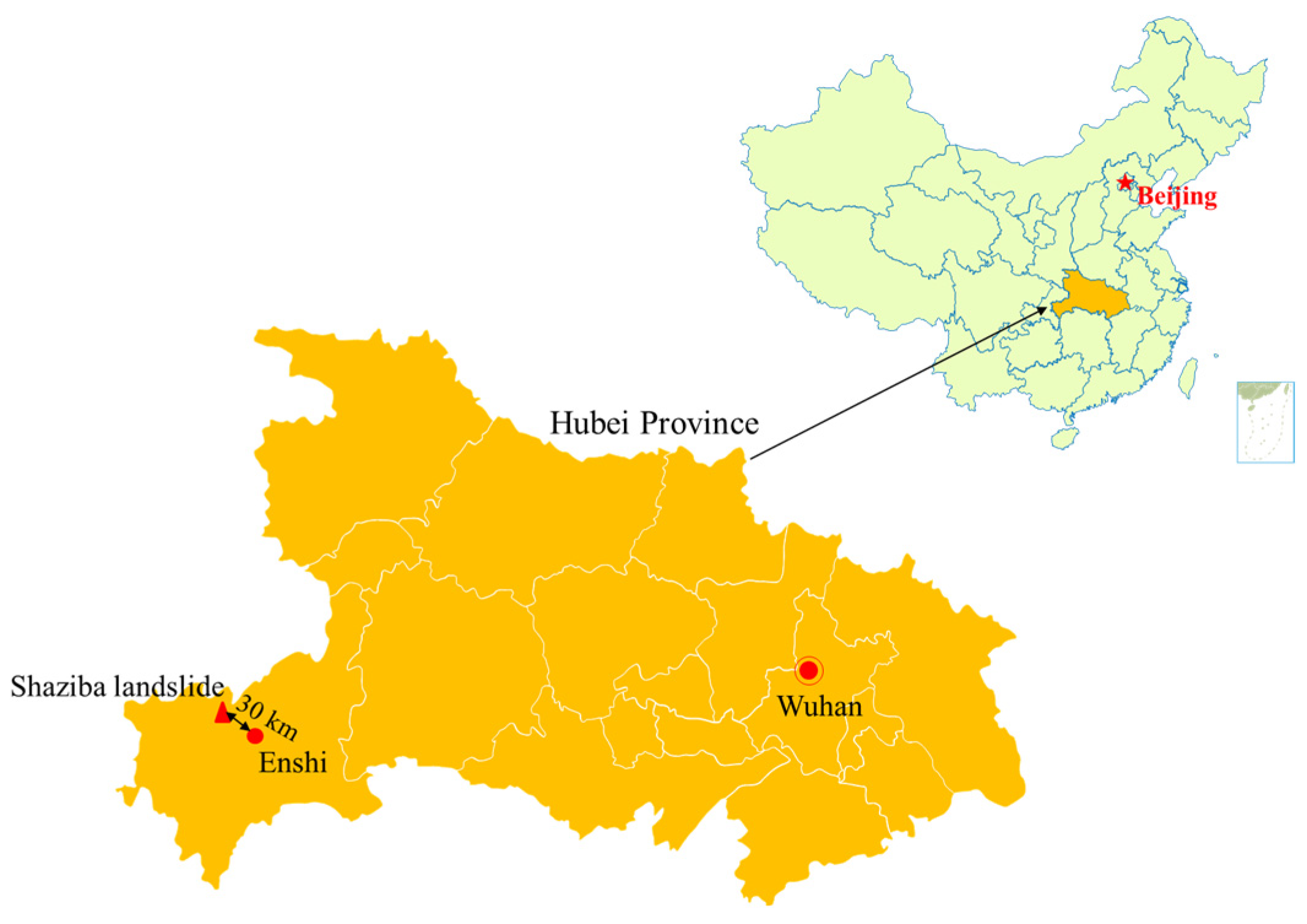
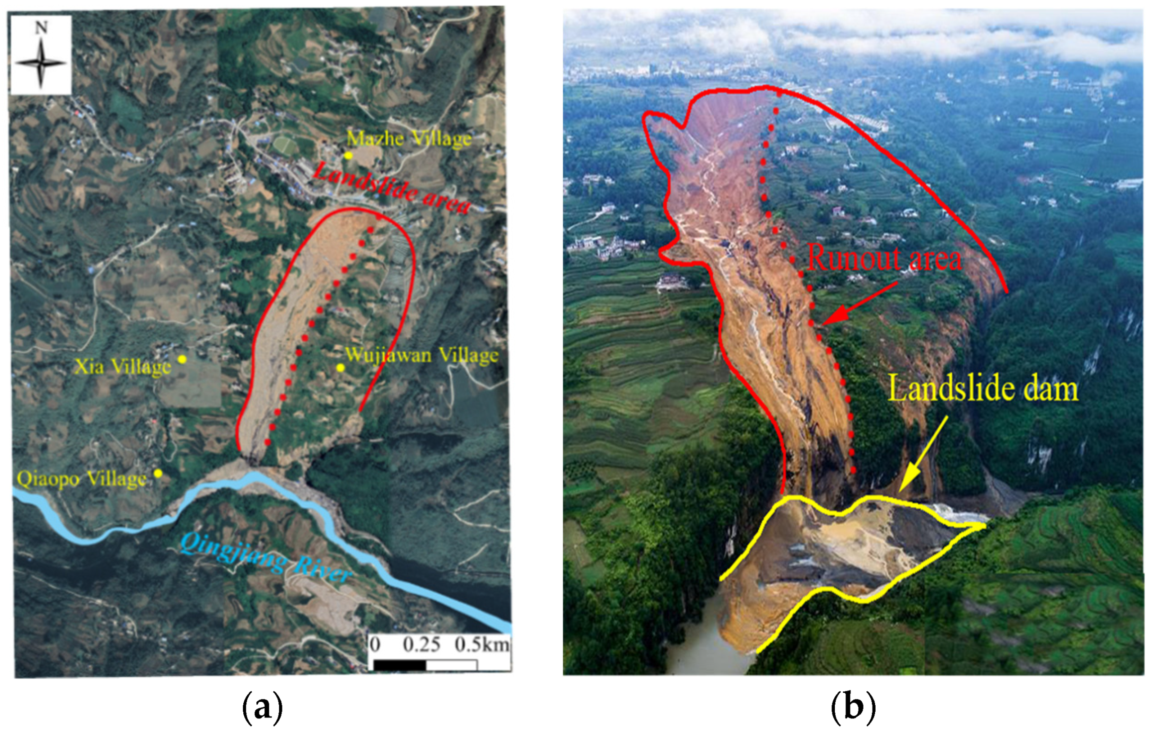
Enshi County is located in the southwest of Hubei Province, China with a geographical latitude of 30°36′5″ N, 109°29′85″ E (Figure 1). This area is dominated by mountainous terrain, and the topography is generally high in the north, northwest, and southeast, and low in the center and south. Enshi has a subtropical monsoon and monsoonal humid climate, with abundant precipitation year-round. The topography and climatic characteristics of Enshi make it prone to geological hazards, particularly landslides [42,43]. At about 5:30 am on 21 July 2020, a large-scale landslide occurred in Shaziba, Mazhe village, about 30 km from Enshi (Figure 1). Mazhe village has more than 1400 residents with a total population of more than 5000 people. It occupies a land area of 33.68 square kilometers with 8828 acres of cultivated land. Mazhe village is rich in selenium elements, which is suitable for the production of tea, tobacco and other economic crops and has important economic value. In addition, the territory is crisscrossed by the Enyu Highway and roads, which provide a good transportation basis for the trade of economic crops. However, this landslide destroyed transportation facilities and fields in the village and eventually blocked the Qingjiang River, seriously threatening the lives and property of 6579 people in 1970 households downstream (Figure 2). Moreover, the disaster caused direct economic losses of over 100 million yuan.
2.2. Geological Condition
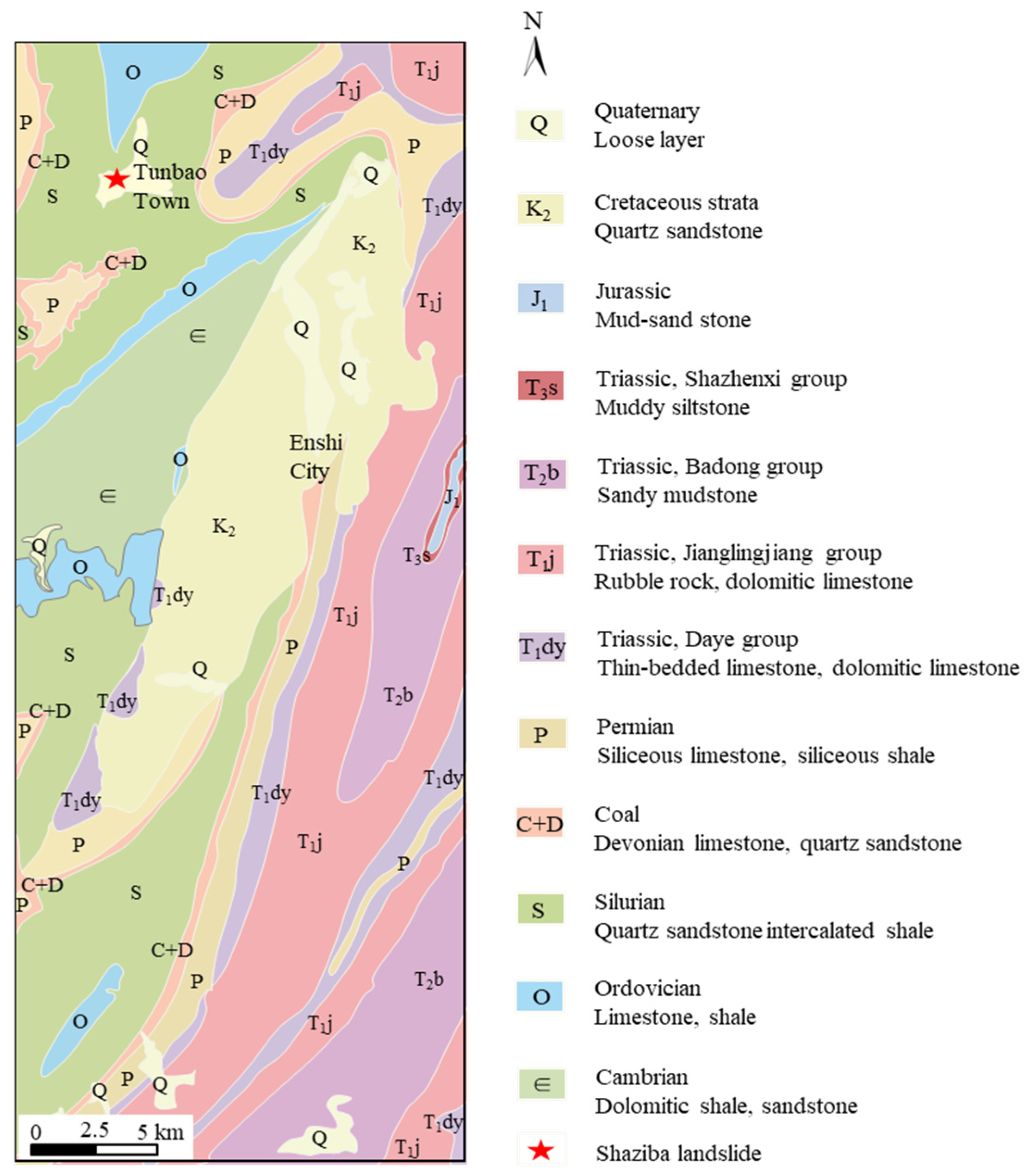
The geological map of the study area is shown in Figure 3. Quaternary loose sediments are widely distributed on the surface of the study area, and the bedrock strata are inter-bedded with Silurian quartz sand stones and shales. The weathering of soft rocks is usually considered as an important factor in the fields of geology, engineering geology and geomorphology. Miscevic and Vlastelica [44] discussed the effect of weathering on slope stability. In the study area, the rock strata area is severely weathered and broken, resulting in the weakness of the rock strata and forming a large amount of loose slope-forming material, which is prone to failure in the rainy season. Peng et al. [43] investigated an area of 1000 km2 in Enshi and analyzed 119 landslides, including the Shaziba landslide. They reported that about 71% of the landslides occurred in two strata: the Silurian strata and the Triassic Badong Formation strata. The Shaziba landslide is located in the Silurian strata. The geological settings in the study area provide abundant loose source material for landslide events.
2.3. Rainfall Characteristics
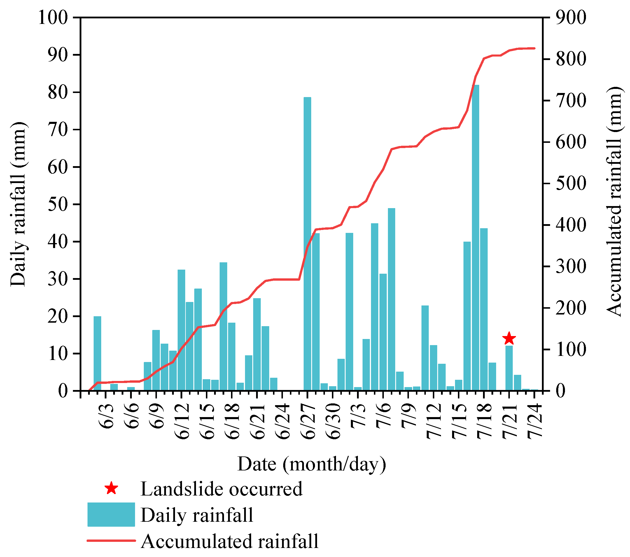
The study area has a typical subtropical monsoon climate with an average annual rainfall of 1500 mm. As shown in Figure 4, the cumulative rainfall in Enshi in the month before the landslide occurrence reached 907 mm, which was the highest monthly precipitation recorded in the past 50 years. In particular, since 15 July 2020, Enshi experienced continuous heavy rainfall, with the highest three days of 16 July (39.8 mm), 17 July (81.8 mm) and 18 July (43.5 mm). As a result, a large-scale landslide was induced at the Shaziba of Mazhe village. Based on the analysis of the relationship between rainfall and landslides in Enshi, Peng et al. [43] classified the rainfall landslides in Enshi area into five different categories. The Shaziba landslide discussed in this paper belongs to the one that was closely related to the cumulative antecedent rainfall before the landslide occurrence. Due to the antecedent rainfall, the slope soil was saturated gradually. In the meantime, the weight of the sliding mass increased and the shear strength of the sliding belt decreased gradually. As a result, the Shaziba landslide occurred under a very small rainfall on 21 July 2020. Therefore, soil saturation was progressive due to antecedent rainfall. Though rainfall on the day of the landslide event was only 10 mm, the antecedent rainfall had already saturated the soil and reduced the stability of the slope to a large extent.
2.4. Landslide Dam
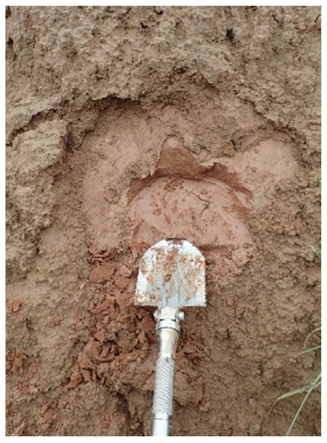
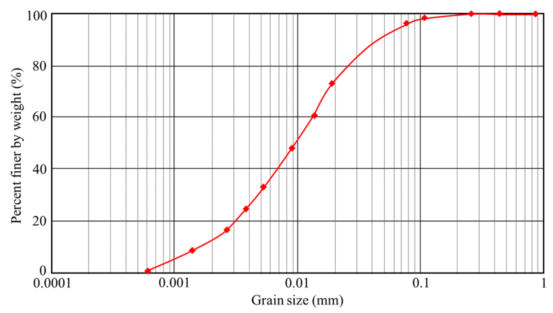
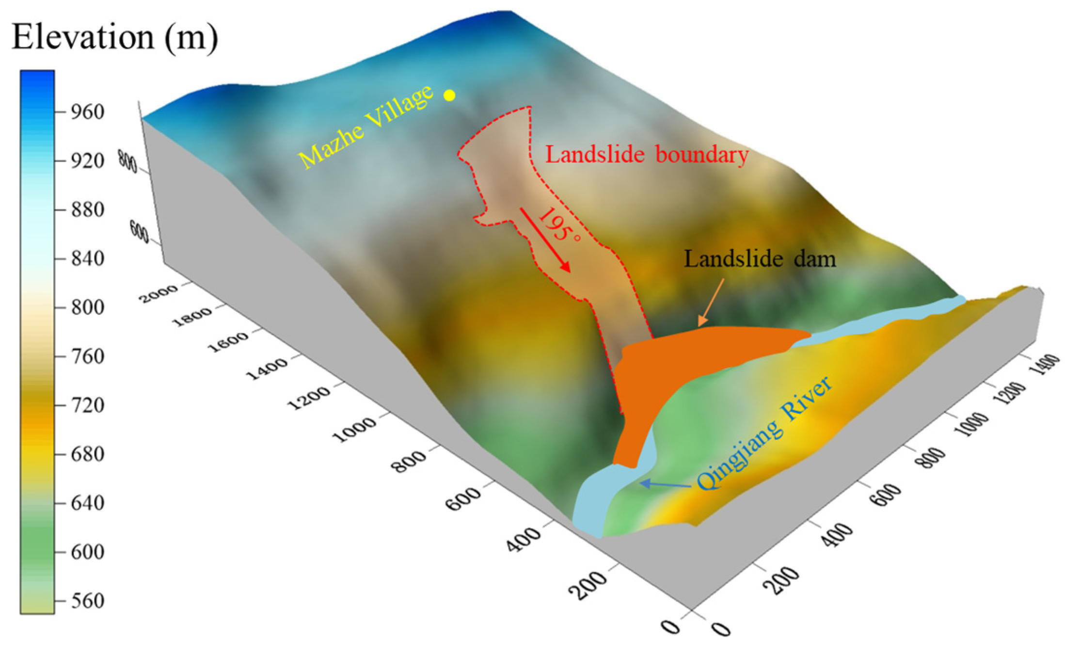
According to the geotechnical material type divisions proposed by Hungr that includes “rock, clay, mud, silt, sand, gravel, boulders, debris, peat” and other material types, the Shaziba landslide can be classified as a gravel–silty clay landslide, of which the geotechnical materials contain silty clay and a few gravels [45]. Figure 5 shows the photo of the silty clay in the landslide site. Figure 6 shows the grain size distribution curve of the silty clay. The plastic limit is 16.52% and the liquid limit is 39.24%. Satellite images (with a resolution of 12.5 m) both before and after the landslide were used to generate the topography model of the slope and identify the landslide boundary, as shown in Figure 7. This shows that the Shaziba slope is located on the right bank of Qingjiang River, with an elevation between 560 m to 960 m. The configuration of the Shaziba landslide was tongue-shaped, and the average slope angle was 10–15°. The sliding direction of the landslide was about 195°, which is approximately consistent with the measured dip angle of the bedrock. The Shaziba landslide had a longitudinal length of 1200 m–1500 m and a transverse width of 320–580 m. The landslide was composed of Quaternary silty clay and a few boulders, with a thickness of 10–43 m and an average thickness of 25 m. The volume of the landslide was approximately 2.8 × 10⁶ m3 [16]. After the landslide, the vegetation was severely damaged, with obvious scars on the left side and sparse vegetation still on the right side (Figure 2).
2.5. Failure Process of the Shaziba Landslide
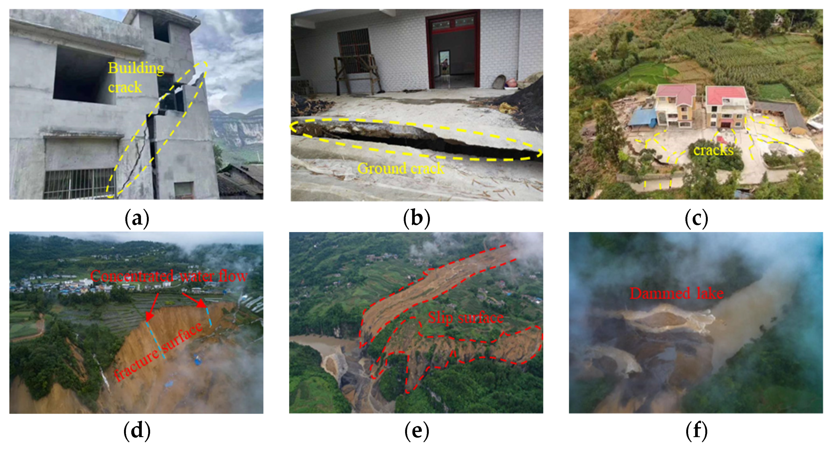
The Shaziba landslide was characterized by progressive failure. As described by local lookout patrols, creep deformation occurred in the slope on 17 July 2020 and cracks appeared on the surface of the ground [16]. The deformation of the landslide intensified on 18 July, causing many cracks in nearby houses and roads (Figure 8a–c). On 19 July, approximately 0.3 × 10⁶ m3 source material on the west of the slope collapsed and flowed downward, some of which slipped into the Qingjiang River. The deformation of the slope developed continuously under the influence of heavy rainfall. Eventually, approximately 2.5 × 10⁶ m3 of source material failed and rushed into the gully at 5:30 am on 21 July 2020. As shown in Figure 2, the gully in the transportation area divided the landslide into two sections. The eastern section had a short moving distance and good integrity, while numerous sliding masses moved outward on the western section, forming a large steep slope. In addition, there were two concentrated flows in the central and western parts of the steep slope, which were the result of surface flows during heavy rainfall (Figure 8d). Under the influence of heavy rainfall and surface flows in the western gully, the sliding mass flowed into the Qingjiang River (Figure 8e,f), forming a landslide dam with a length of 60–80 m, a width of 300–350 m wide, and a height of 8–10 m. The Shaziba landslides caused serious damage to the surrounding farmland, vegetation, houses, and infrastructure.
3. Methodology
3.1. PFC Theory
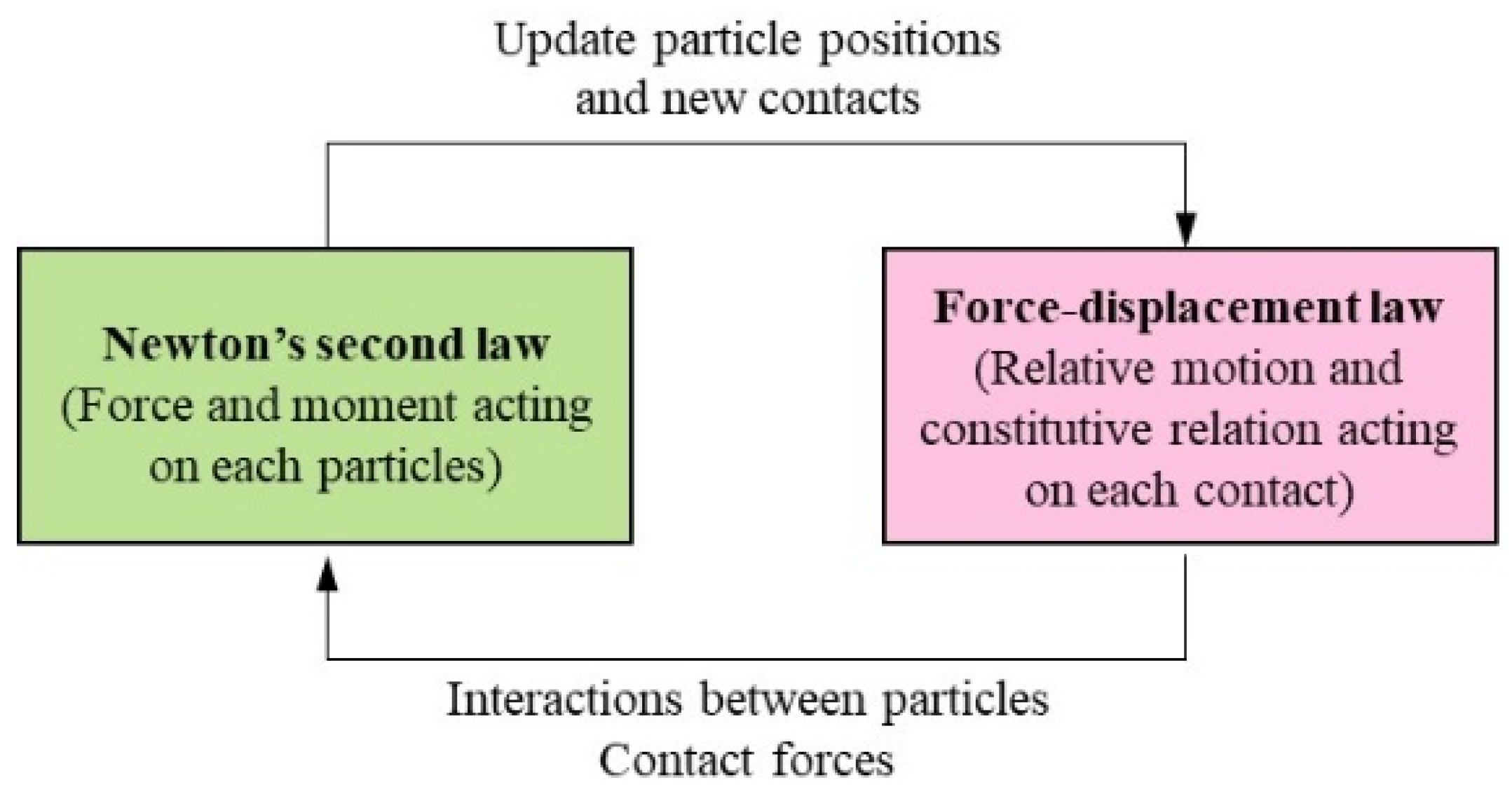
PFC is a computing software developed by the American Itasca company. It was initially proposed to analyze the mechanical properties of soil particles by Cundall and Strack [46]. As a numerical software based on the discrete element method, PFC has been widely used in the field of geotechnical engineering to study the mechanical properties and deformation behavior of rock and soil mass, which are simplified as a granular system in the simulation. The basic element of PFC is a sphere (circle in 2D) carrying the physical properties of the material and interacting with other elements. PFC3D is a three-dimensional version of the software able to analyze complex motions of geo-material on a 3D terrain [47,48]. In the PFC3D model, the geo-material is composed of rigid particles. It can not only directly simulate the movement and interaction of each particle, but also form a combination of optional shapes by connecting any particle with its adjacent particles to simulate a block structural issue. PFC3D uses the wall as the constraint of particle motion. The mechanical relationship between the particles obeys Newton’s second law. The contact force is simulated by the overlap between the particles, allowing limited displacement and rotation, and the particles can be completely separated due to the theory of discontinuities. During the calculation process, new contacts can be automatically identified. The mechanical properties of the geo-material depend on the structure and contact characteristics of the particles. According to the time-step calculation principle and Newton’s second law, it calculates the contact motion, whether particle-to-particle or particle-to-wall [49,50]. In the PFC model, the time-step calculation is automatic and includes the effects of changing stiffnesses due to the contact model. Additionally, during the simulation, the time-step changes with the contact numbers and instantaneous stiffness of the particles. As shown in Figure 9, the model of particles and walls is first established to form the initial contact. During the first time-step, contact generates force and moment on each particle, and Newton’s second law is applied to update the velocity and position of the particles. Next, the force–displacement law is used to update contact forces through relative motion and the constitutive relationships of adjacent entities, which act at each contact. The calculation is repeated at the beginning of each time step until the unbalanced force between particles is less than the set value.
3.2. Model Establishment
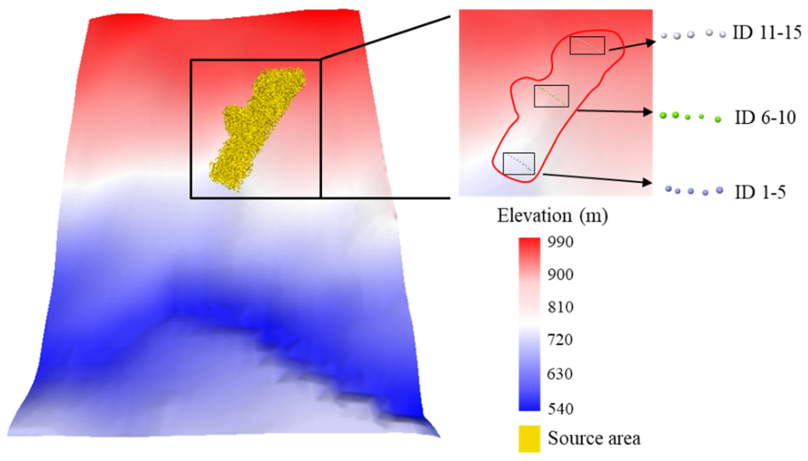
In this study, the numerical model of the Shaziba landslide was established using the Ball-Wall mode. This model uses rigid spherical particles to simulate the sliding body, and the 3D terrain is represented by a series of wall elements. Compared with other modes, the Ball-Wall mode generates fewer particles for the numerical model and significantly improves the computational efficiency. In addition, this method is suitable for landslides of which the sliding surface is determined. The volume of the landslide body was determined to be about 2.8 × 10⁶ m3 based on the field investigation. The calculation accuracy of the PFC model increases when using fine particles, while the computational efficiency decreases sharply when increasing the particle numbers. Therefore, to balance the calculation accuracy and efficiency, the Shaziba landslide was discretized into a total of 13,136 particles with a diameter of 2–2.5 m by using the Ball-Wall mode. The density of the material was 2.1 × 10³ kg/m3. As shown in Figure 10, the sliding surface of the Shaziba landslide was composed of 696,129 wall elements. To capture the evolution of displacement and velocity during landslide propagation, a total of 15 monitored particles were placed in the front, middle and rear parts of the sliding body respectively (Figure 10).
The landslide material is usually very complicated, including the three phases of gas, liquid, and solid. The interaction of different phases may influence the macro-mechanical property of the geo-material. Therefore, it is better to simulate the mechanical behavior of soils using a multi-phase coupled model. However, for large-scale events such as flow-like landslides, it is difficult to quantitatively consider the micro-interaction among different phases when modeling the propagation behavior of landslides. Therefore, the propagation behavior of flow-like landslides is usually simulated as a single-phase viscous fluid in the literature. For example, Hungr [51] proposed a DAN model based on integrated “shallow-flow” theory to simulate flow-like landslides. In this model, the landslide material was assumed to be a single-phase “equivalent fluid”, which was evidenced to be highly efficient. Huang et al. [52] proposed an SPH model to predict the runout distance of flow-like landslides. The flow-like landslides were simulated as a single-phase Bingham fluid, and the accuracy of the modeling results was verified. Li et al. [53] simulated the runout behavior of the Jiweishan landslide using a single-phase model based on PFC and verified the efficiency of the solver. Similar research work can be found in [54,55,56]. Therefore, in the presented study, the propagation of the Shaziba landslide was assumed to be a single-phase material for simplified calculation and the material’s multi-phase nature was ignored, though the source material of the Shaziba landslide was saturated soil containing water and soil phases.
In the PFC model, the parallel bonding model can well simulate the mechanical properties of cohesive soils, such as inter-granular tensile, shear and bending moments. Therefore, it was used in this study to consider the interaction between particles and simulate the dynamic behavior of the saturated sliding body.
3.3. Calibration of Parameters
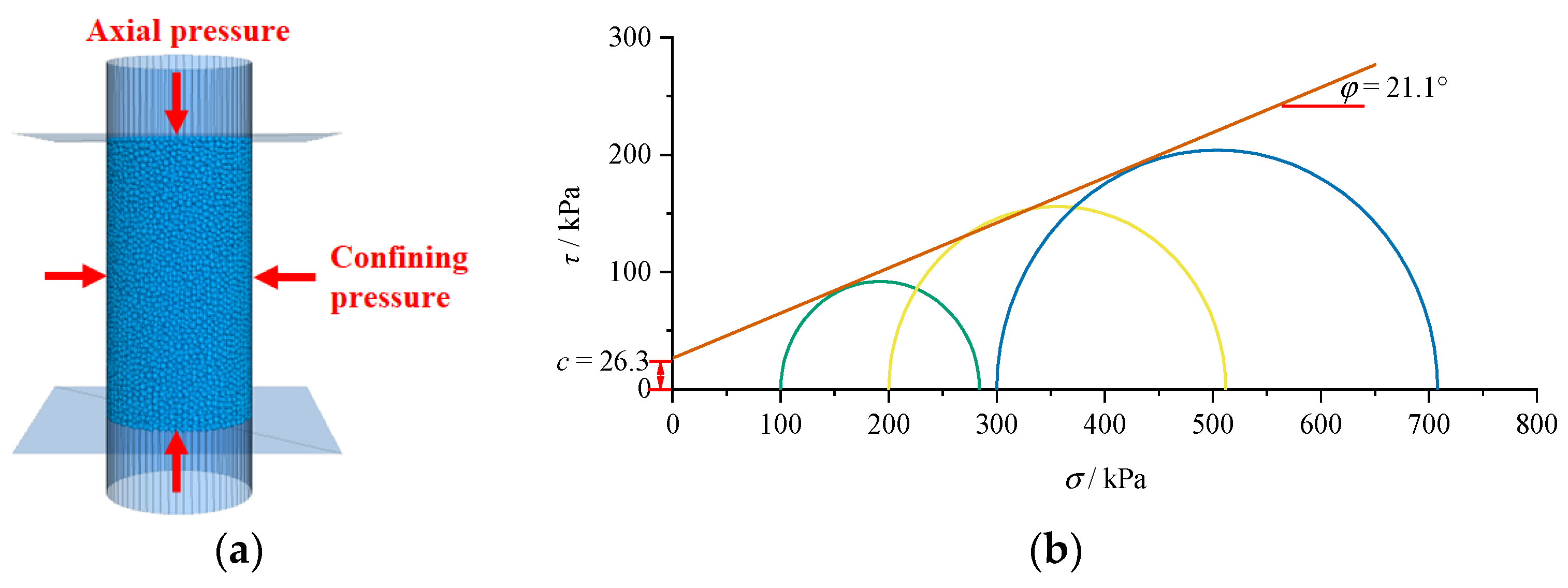
In the PFC model, the macroscopic mechanical behavior of geo-materials is determined by the micro-mechanical properties of granular assembly. However, the determination of these micro-parameters is a challenge with various uncertainties, since they cannot be directly obtained in the laboratory tests, and no complete theory can reliably predict macroscopic behavior from microscopic properties and geometry. The most efficient approach so far involves a trial-and-error process. In the literature, virtual compressive strength tests have been widely performed to calibrate the micro-parameters of PFC models. For example, Tang et al. [55] performed a series of numerical biaxial tests on granular samples to calibrate the PFC parameters before modeling the Tsaoling landslide. Li et al. [53] conducted virtual uniaxial compression tests for parameter calibration before the PFC simulation of the Jiweishan landslide. Similar research works can be found in some recent literature [18,57]. The effectiveness of this method has been validated through the above research works. Therefore, in this study, a series of numerical biaxial compression tests were performed on granular samples to calibrate the parameters used in the PFC simulation, as shown in Figure 11a. The parameters used in the simulations are shown in Table 1. By controlling the confining pressure to be 100 kPa, 200 kPa and 300 kPa, respectively, the Mohr’s circles of the granular assembly under different stress states were obtained as well as the Mohr failure envelope, shown in Figure 11b. From this, the cohesion (c) and internal friction angle (φ) of the granular assembly can be calculated to be 26.3 kPa and 21.1°, respectively. According to the literature [57,58], the cohesion of Quaternary silty clay in the study area is 22–37 kPa, and the internal friction angle is 18–25°. Therefore, the shear strength characteristic of the granular assembly in the PFC model is consistent with that of the source material of the Shaziba landslide. It can be concluded that the PFC particles with the micro-mechanical parameters shown in Table 1 can be used to simulate the mechanical behavior of the source material of the Shaziba landslide.
4. Results
4.1. Kinetic Process of the Shaziba Landslide
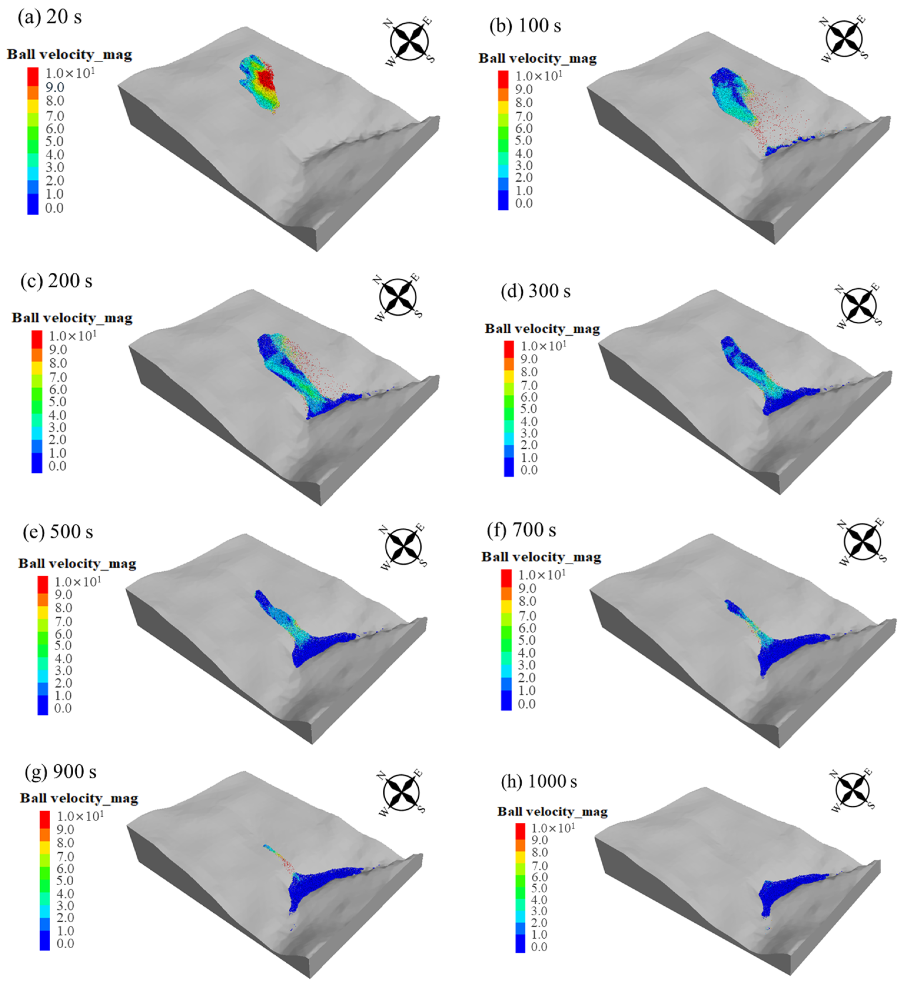
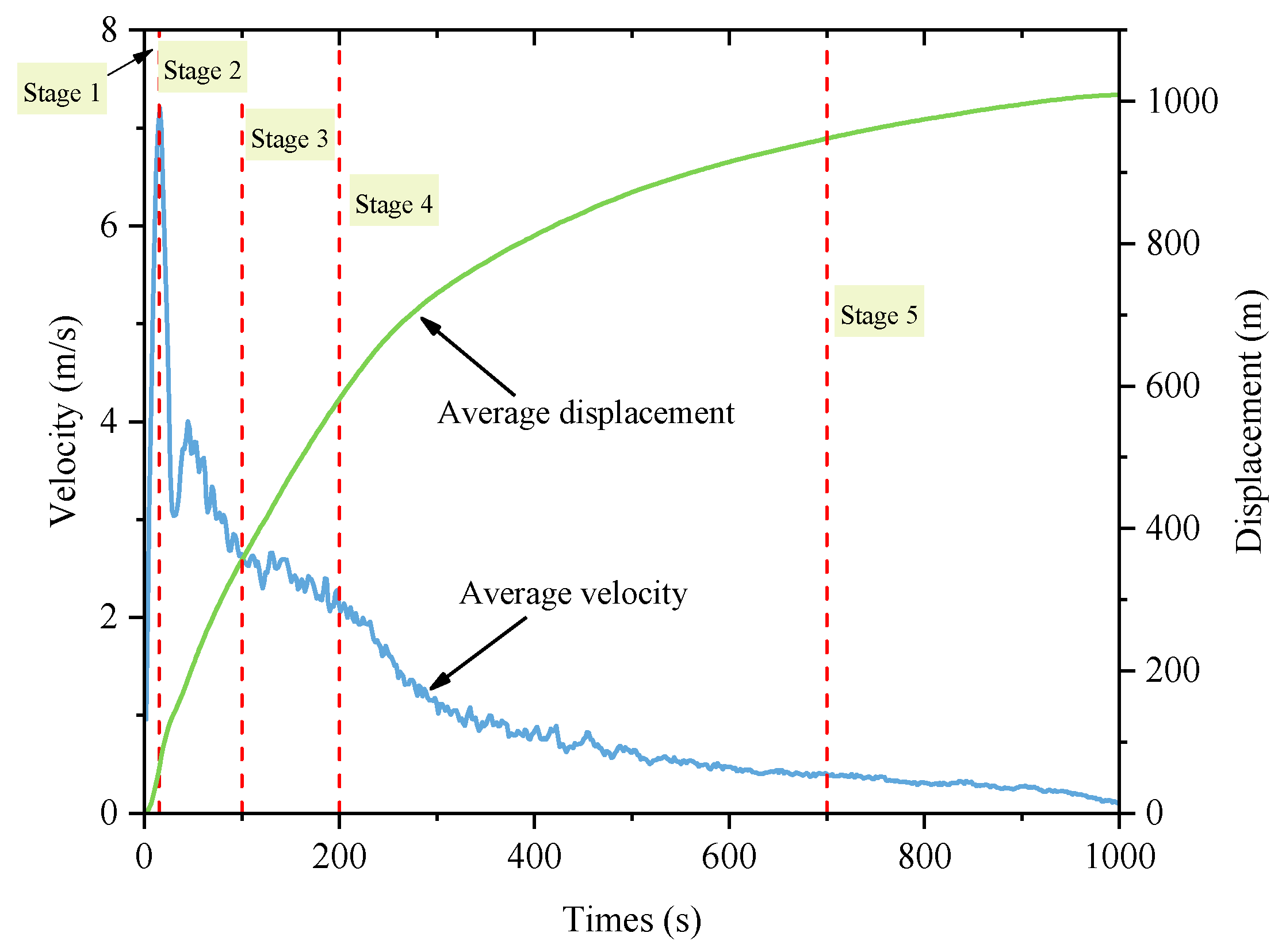
In July 2020, the continuous rainfall in Enshi saturated the soils and increased the pore pressure ratio gradually. Then, the matrix suction in the unsaturated zone reduced and the effective stress of the slope forming material decreased. As a result, the shear strength of the soil in the sliding belt of the slope decreased, which resulted in the landslide event. The dynamic movement of the Shaziba landslide simulated using the PFC3D is shown in Figure 12. After being triggered by continuous rainfall, the landslide moved rapidly downward. The whole process lasted approximately 1000 s, which can be divided into five stages: (1) For the first 20 s, the slope failure occurred along the sliding surface and a rapid downward movement began (Figure 12a). (2) From 20 s to 100 s, the northeastern part of the trailing edge was first separated from the slope. This part was located on flat terrain. After failure, the sliding mass quickly moved to the southeast over the lower terrain. At the same time, the velocity of the landslide rapidly increased. The maximum velocity exceeded 14 m/s and the average velocity also rapidly increased to approximately 7.5 m/s. The remaining parts of the sliding mass gathered and constantly moved downward (Figure 12b). (3) During the period of 100 s to 200 s, the northeastern part of the trailing edge completely separated from the slope and began to accumulate downstream near the Qingjiang River. The velocity also gradually decelerated to 2–4 m/s. The trailing edge of the sliding body formed a distinct steep scarp. The rest of the sliding mass continued to move downward until it reached the channel and gradually accumulated (Figure 12c). (4) In the propagation of the landslide, the velocity gradually decreased due to the collision and friction between particles. Most of the sliding mass began to accumulate in the downstream river channel. (Figure 12d,e). (5) After 700 s, most of the sliding mass had stopped moving and accumulated at the foot of the slope, and only a small amount of sliding mass continued to move down (Figure 12f,g). Finally, the sliding mass was deposited along the channel (Figure 12h). The time history of the average velocity and displacement of soil mass during different stages are shown in Figure 13. The velocity change at each stage is consistent with that in Figure 12. During the whole process, the peak velocity of the landslide body appeared in the second stage, which was 7.5 m/s, and the average runout distance of the landslide exceeded 1000 m.
4.2. Landslide Runout Behavior
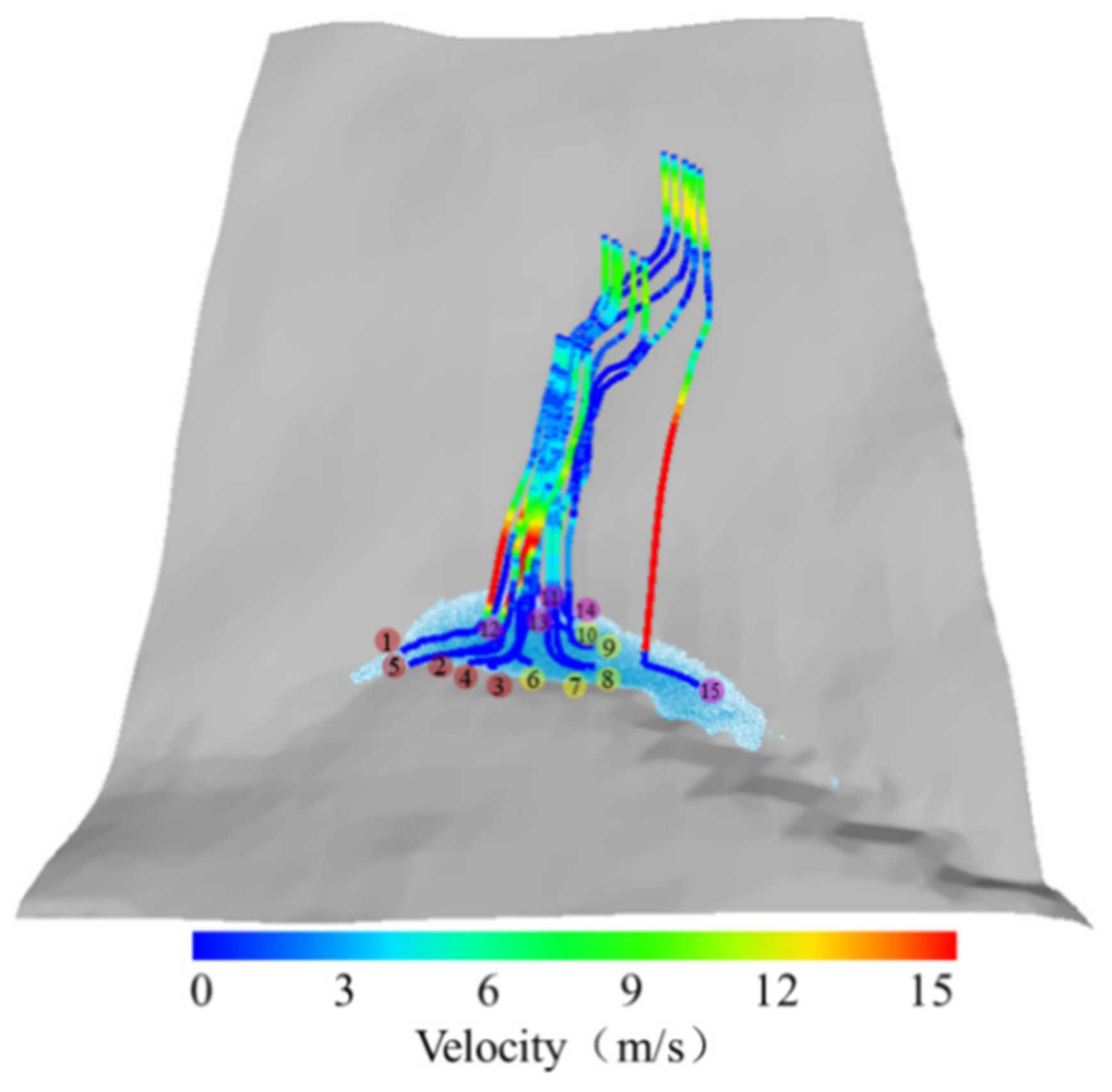
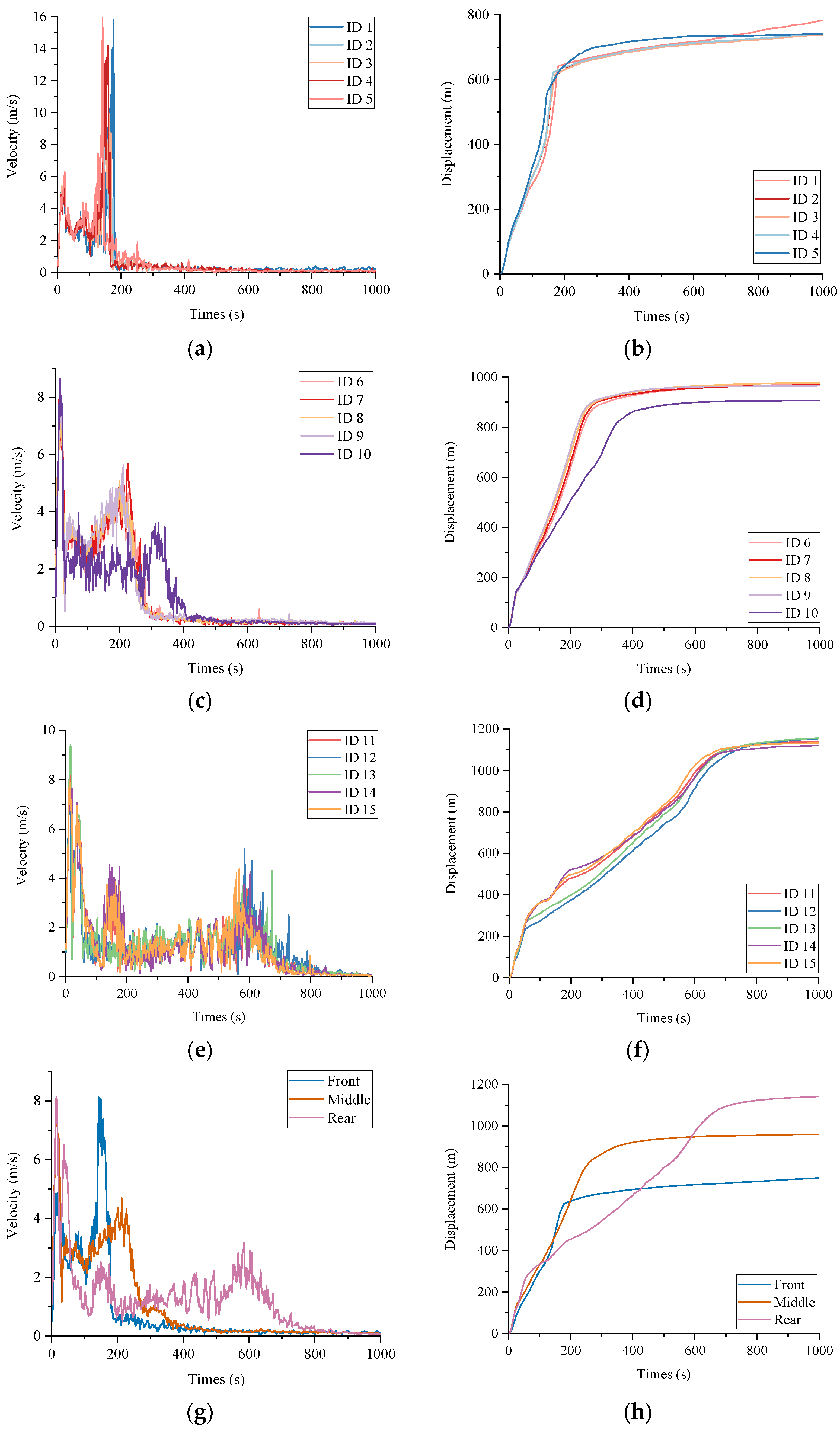
To observe the detailed information of the landslide propagation, 15 monitored particles were set in the front, middle and rear parts of the sliding body, respectively. The trajectories of each monitored particle are shown in Figure 14, and the evolution of velocity and displacement is shown in Figure 15. It is obvious that the velocity of the monitored particles in the front was the largest. It reached a peak value of 16 m/s between 100 s and 200 s. During this time, the front particles moved rapidly towards the lower terrain. The displacement of the particles rapidly increased approximately linearly with time. Due to the gentle terrain at the foot of the slope, the velocity of the particles decreased rapidly until they came to a complete standstill (Figure 15a,b). In addition, the velocity of the particles in the middle and rear parts increased less than that of the front particles (Figure 15a–f). There are two peaks in the velocity histories of the particles in the middle part. The first peak occurred within the first 20 s. During this time, the motion of the particles in the middle parts was affected by the terrain. They collided and moved downwards. The velocity increased rapidly at short times, and the displacement increased linearly. The velocity of the particles gradually decreased as they moved into the flat terrain. At the same time, the inter-particle collisions were also weakened. After 300 s, the velocity reached a second peak as the particles travelled down the steep slope above the channel (Figure 15c). The motion process of the rear part of the sliding mass was similar to the middle part. Due to the higher initial elevation of these particles, the second velocity peak occurred later and the particles traveled the longest distance when they reached the river channel (Figure 15e,f). As shown in Figure 15g, there were two peaks in the velocity histories of all the monitored particles. In the initial stage, the landslide disintegrated and the particles collided violently. As a result, the velocity increased significantly and the first peak occurred. The second peak occurred when the particles rushed down the steep slope above the river channel. Eventually, all the particles stopped moving and piled up on the river bed (Figure 14).
4.3. The Morphology of the Landslide Deposits
In this study, the final morphology of the landslide deposits refers to the geometry of the sliding mass accumulated in the Qingjiang river channel. The morphology of the landslide deposits is usually described by the geometrical parameters of length, width and height. The final morphology of the Shaziba landslide obtained from the simulation is shown in Figure 16. The maximum length (B-b) and width (A-a) of the landslide deposits are approximately 386 m and 127 m, respectively. In addition, as shown in the profile of section A-a, affected by the river channel, the depth of the landslide deposits reaches a maximum of 19 m in the central part. The profile of section B-b shows that the depth of the landslide deposits is almost uniform, and the maximum depth is approximately 18 m. In general, deposits expand along the river channel from middle to both sides. The depth of the landslide deposits is larger in the lower places, and the area of deposits gradually decreases as the terrain increases. Figure 17 shows the simulated and measured landslide deposit area in the contour map of the slope. Through the comparison, it shows that the simulated landslide dam shape is in agreement with the measured results, though the size of the simulated dam is a little larger than the measured one.
5. Discussion
In this section, the mechanism of the landslide is further discussed based on the results of field investigations and numerical simulations. Moreover, numerical simulations of the Shaziba landslide were performed using different effective modulus to further discuss the effect of this parameter on the landslide propagation.
5.1. Mechanism of the Landslide
Landslides can be induced by many factors, such as rainfall, earthquakes and human activities [59,60]. Continuous rainfall can easily induce landslides, causing serious damage to the surroundings [61,62]. The study area Enshi was hit by heavy rainfall in the week before the Shaziba landslide occurrence. When rainfall infiltrates into the unsaturated soil of a hillslope, the increased water content of the soil leads to a loss of matric suction and then reduces the strength of the soil mass. On the other hand, the rainfall increases the soil weight and causes deformation of the slope, eventually triggering large-scale landslides. The results presented in this study show that the mechanism of the Shaziba landslide can be summarized as follows: (1) The average slope angle of the landslide area was 10–15°, and the sliding direction was consistent with the dip angle of the bedrock. Moreover, there was a nearly vertical scarp at the foot of the slope (Figure 8e), providing favorable terrain for landslide occurrence. In addition, the bedrock of the study area was dominated by Silurian strata, and the Quaternary deposits were widely distributed on the surface. The geological conditions made the study area prone to landslides. (2) Field investigation results show that the central and western parts of the Shaziba slope area had already experienced gradual deformation during the past years. The slope deformation was sensitive to seasonal variations, which are most pronounced during the rainy season. A week of heavy rainfall totally saturated the soils at the landslide location and greatly increased the underground water level. As a result, the effective stress and shear strength of the sliding zone soil decreased, and then triggered the slope failure. (3) After the slope failure, a steep scarp was formed on the trailing edge of the landslide (Figure 8d). Rainwater and surface water flows were rapidly accumulated. As a result, large amounts of water flowed into the landslide, significantly increasing the mobility of the landslide body and accelerating the movement. In conclusion, rainfall is a significant trigger of landslide disaster. Therefore, establishing a rainfall threshold for landslide occurrence at the regional level can contribute to disaster prediction and early warning.
5.2. Influence of the Effective Modulus on Landslide Propagation
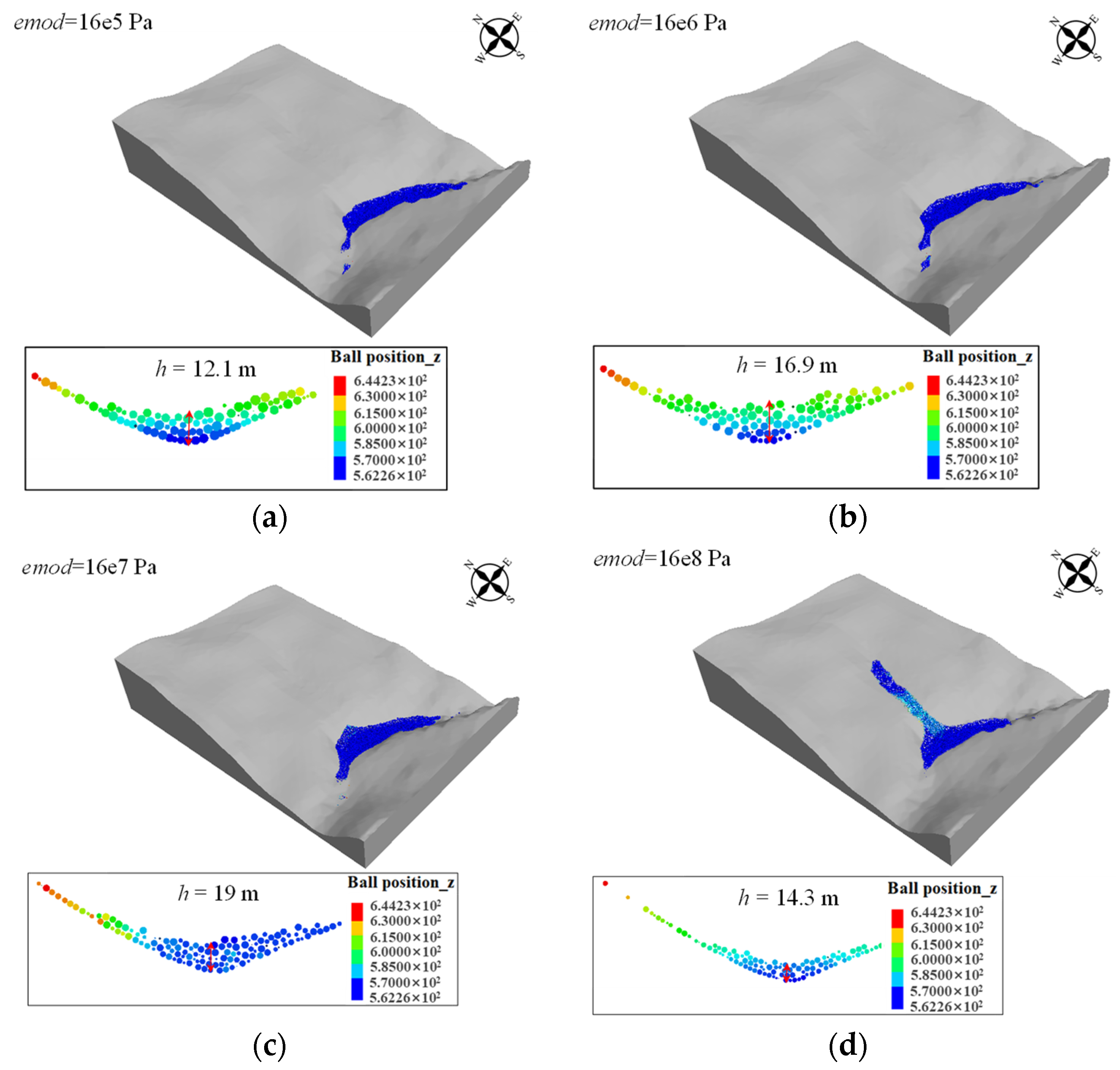
The contact mode between particles (i.e., the collision and the friction) affects the dynamic behavior of particle system. The effective modulus is a key parameter of the contact model used in this work. Therefore, to further study the influence of the effective modulus on the propagation behavior of landslides, its value was set to 16 × 105 Pa, 16 × 106 Pa, 16 × 107 Pa, and 16 × 108 Pa, respectively. The final accumulation area, average velocity, and runout displacement of the landslide under different effective modulus are shown in Figure 18. When the effective modulus was set to 16 × 105 Pa, the particle system was loosely distributed in the accumulation areas. As the effective modulus increases, the distribution of particle system becomes more concentrated, and the height of the final landslide deposits increases (Figure 18a–d). Particularly, when the effective modulus increased to 16 × 108 Pa, due to the close contact of the particles, the velocity of the landslide significantly decreased. As a result, a large number of particles could not reach the river channel (Figure 18d). The results evidently show that the runout behavior of a landslide and the morphology of landslide deposits are closely related to the effective modulus in the contact model.
5.3. Limitations of the Modeling Approach
As a numerical software based on the DEM method, the PFC3D introduced in this study has obvious advantages in modeling extremely large deformation behaviors of geo-material. Therefore, it has been widely applied in the simulation of geological disaster propagation, such as flow-like landslides [53,57], rock avalanches [63,64], and debris flows [41,65] with both dry and saturated source materials. The validity and reliability of the PFC models have been extensively verified.
However, the limitations of the PFC model come to light during the application to a variety of landslide case studies. First, the relationship between the micro-parameters of the PFC particles with the macro-mechanical properties of the granular assembly remains unknown [66]. The determination of the micro-parameters in the model still needs theoretical support. Second, some important phenomena involved in landslide propagation, such as multi-phase interaction [67,68] and bed entrainment [69] are observed in field investigation but cannot be considered in the presented PFC model. Therefore, the performance of the model should be improved and further verified. Third, for rainfall-induced landslides, the shear strength of soil along the slip surface varies during rainfall due to the development of pore pressure. In the presented PFC model, the parameters of the soil keep the same during the simulation of landslide propagation, which may result in some numerical error. In addition, the computation efficiency of the PFC3D is quite low when a large number of PFC particles are generated for the three-dimensional modeling of large-scale landslides. Therefore, although the simulation results in this study are acceptable, much more attention and efforts should be paid to break through the above limitations and improve the model performance.
6. Conclusions
The Shaziba landslide was a typical rainfall-induced landslide in Enshi County, China that caused great damage to surrounding roads and buildings. To investigate the post-failure behavior of this landslide, a three-dimensional numerical model based on the PFC3D was presented to simulate the propagation of the landslide. The main conclusions drawn from this study are as follows:
- (1)
- The Shaziba landslide is located in an area of Silurian strata, which is prone to landslides. Due the continuous heavy rainfall, the precipitation infiltration caused slope failure and triggered the large-scale landslide. After the landslide occurred, a steep scarp was formed on the trailing edge of the landslide. The sliding mass rushed into the Qingjiang River channel. Finally, a landslide dam formed, causing significant damage to the surroundings.
- (2)
- The simulation results show that the whole process of the Shaziba landslide took approximately 1000 s. It can be divided into five stages: early accelerated deformation, disintegration at the trailing edge of the slide, runout along the main sliding surface, decelerated movement and final deposition stage. The average velocity of the landslide could reach up to 7.5 m/s, and the average displacement was approximately 1000 m. The landslide piled up along the Qingjiang River valley after the movement stopped. The thickness of the landslide deposits gradually decreased from the center to the sides. The maximum height of the landslide deposits was about 19 m. The length and width were approximately 108–127 m and 328–386 m, which is in good agreement with the field investigations.
- (3)
- The runout behavior of a landslide and the morphology of landslide deposits are closely related to the effective modulus in the contact model of the PFC3D. As the effective modulus increases, the distribution of particles becomes more concentrated, and the height of the final landslide deposits increases. However, the velocity of the landslide significantly reduces.
- (4)
- The results achieved in this study show that the PFC3D model can provide an effective tool for investigating the dynamic features of flow-like landslides and a means for mapping hazardous areas and estimating hazard intensity.
Author Contributions
Conceptualization, H.C. and Z.D.; methodology, Z.D.; software, L.W.; validation, H.C., L.W. and Z.D.; data curation, H.C., and L.W.; writing—original draft preparation, L.W.; writing—review and editing, H.C., and Z.D.; supervision, Z.D.; funding acquisition, Z.D. All authors have read and agreed to the published version of the manuscript.
Funding
The research work herein was supported by the National Natural Science Foundation of China (grant No. 42102318) and the Program for Professor of Special Appointment (Eastern Scholar) at the Shanghai Institutions of Higher Learning.
Data Availability Statement
The data presented in this study are all available on request.
Conflicts of Interest
The authors declare no conflict of interest.
References
- Evans, S.G.; Degraff, J.V. Catastrophic Landslides; Geological Society of America: Boulder, CO, USA, 2002. [Google Scholar]
- Iverson, R.M. Landslide triggering by rain infiltration. Water Resour. Res. 2000, 36, 1897–1910. [Google Scholar] [CrossRef] [Green Version]
- Yin, Y.P.; Cheng, Y.; Liang, J.; Wang, W. Heavy-rainfall-induced catastrophic rockslide debris flow at Sanxicun, Dujiangyan, after the Wenchuan Ms 8.0 earthquake. Landslides 2015, 13, 9–23. [Google Scholar] [CrossRef]
- Gao, Y.; Li, B.; Gao, H.; Chen, L.; Wang, Y. Dynamic characteristics of high-elevation and long-runout landslides in the Emeishan basalt area: A case study of the Shuicheng “7.23” landslide in Guizhou, China. Landslides 2020, 17, 1663–1677. [Google Scholar] [CrossRef]
- Chen, G.Q.; Xia, M.Y.; Thuy, D.T.; Zhang, Y.B. A possible mechanism of earthquake-induced landslides focusing on pulse-like ground motions. Landslides 2021, 18, 1641–1657. [Google Scholar] [CrossRef]
- Liu, B.; Hu, X.; He, K.; Li, G.; Liu, X.; Luo, G.; Xi, C.J.; Zhou, R.C. Preliminary analyses of the Tiejiangwan landslide occurred on April 5, 2021 in Hongya County, Sichuan Province, China. Landslides 2022, 19, 2047–2051. [Google Scholar] [CrossRef]
- Dai, Z.L.; Huang, Y.; Cheng, H.L.; Xu, Q. 3D numerical modeling using smoothed particle hydrodynamics of flow-like landslide propagation triggered by the 2008 Wenchuan earthquake. Eng. Geol. 2014, 180, 21–33. [Google Scholar] [CrossRef]
- Pastor, M.; Haddad, B.; Sorbino, G.; Cuomo, S.; Drempetic, V. A depth-integrated, coupled SPH model for flow-like landslides and related phenomena. Int. J. Numer. Anal. Methods Geomech. 2009, 33, 143–172. [Google Scholar] [CrossRef]
- Muceku, Y.; Korini, O. Landslide and slope stability evaluation in the historical town of Kruja, Albania. Nat. Hazards Earth Syst. Sci. 2014, 14, 545–556. [Google Scholar] [CrossRef] [Green Version]
- Fan, X.M.; Xu, Q.; Scaringi, G.; Dai, L.X.; Li, W.L.; Dong, X.J.; Zhu, X.; Pei, X.J.; Dai, K.R.; Havenith, H.B. Failure mechanism and kinematics of the deadly June 24th 2017 Xinmo landslide, Maoxian, Sichuan, China. Landslides 2017, 14, 2129–2146. [Google Scholar] [CrossRef]
- Xin, P.; Liang, C.; Wu, S.; Liu, Z.; Shi, J. Kinematic characteristics and dynamic mechanisms of large-scale landslides in a loess plateau a case study for the north bank of the Baoji stream segment of the Wei River, China. Bull. Eng. Geol. Environ. 2016, 75, 659–671. [Google Scholar] [CrossRef]
- Zhou, J.W.; Cui, P.; Hao, M.H. Comprehensive analyses of the initiation and entrainment processes of the 2000 Yigong catastrophic landslide in Tibet, China. Landslides 2015, 13, 39–54. [Google Scholar] [CrossRef]
- Ma, J.; Tang, H.; Hu, X.; Bobet, A.; Yong, R.; Ez Eldin, A.M. Model testing of the spatial–temporal evolution of a landslide failure. Bull. Eng. Geol. Environ. 2016, 76, 323–339. [Google Scholar] [CrossRef]
- Zhang, Z.; Wang, T.; Wu, S.; Tang, H.; Liang, C. Investigation of dormant landslides in earthquake conditions using a physical model. Landslides 2017, 14, 1181–1193. [Google Scholar] [CrossRef]
- Pei, X.; Guo, B.; Cui, S.; Wang, D.; Xu, Q.; Li, T. On the initiation, movement and deposition of a large landslide in Maoxian County, China. J. Mt. Sci. 2018, 15, 1319–1330. [Google Scholar] [CrossRef]
- Shen, D.Y.; Shi, Z.M.; Peng, M.; Zhang, L.M.; Zhu, Y. Preliminary analysis of a rainfall-induced landslide hazard chain in Enshi City, Hubei Province, China in July 2020. Landslides 2021, 4, 509–512. [Google Scholar] [CrossRef]
- Zhou, J.W.; Huang, K.X.; Shi, C.; Hao, M.H.; Guo, C.X. Discrete element modelling of the mass movement and loose material supplying the gully process of a debris avalanche in the Bayi Gully, Southwest China. J. Asian Earth Sci. 2015, 99, 95–111. [Google Scholar] [CrossRef]
- Wei, J.; Zhao, Z.; Xu, C.; Wen, Q. Numerical investigation of landslide kinetics for the recent Mabian landslide (Sichuan, China). Landslides 2019, 16, 2287–2298. [Google Scholar] [CrossRef]
- Deng, Q.; Gong, L.; Zhang, L.; Yuan, R.; Xue, Y.; Geng, X.; Hu, S. Simulating dynamic processes and hypermobility mechanisms of the Wenjiagou rock avalanche triggered by the 2008 Wenchuan earthquake using discrete element modelling. Bull. Eng. Geol. Environ. 2017, 76, 923–936. [Google Scholar] [CrossRef]
- Hu, X.; Fan, X.; Tang, J. Accumulation characteristics and energy conversion of high-speed and long-distance landslide on the basis of DEM: A case study of Sanxicun landslide. J. Geomech. 2019, 25, 527–553. [Google Scholar]
- Lo, C.M.; Huang, W.K.; Lin, M.L. Earthquake-induced deep-seated landslide and landscape evolution process at Hungtsaiping, Nantou County, Taiwan. Environ. Earth Sci. 2016, 75, 645. [Google Scholar] [CrossRef]
- Fei, J.B.; Chen, T.L.; Jie, Y.X.; Zhang, B.Y.; Fu, X.D. A three-dimensional yield-criterion-based flow model for avalanches. Mech. Res. Commun. 2016, 73, 25–30. [Google Scholar] [CrossRef]
- Ozbay, A.; Cabalar, A.F. FEM and LEM stability analyses of the fatal Landslides at Collolar open-cast lignite mine in Elbistan, Turkey. Landslides 2016, 12, 155–163. [Google Scholar] [CrossRef]
- Moayedi, H.; Huat, B.B.K.; Ali, T.A.M.; Asadi, A.; Moayedi, F.; Mokhberi, M. Preventing landslides in times of rainfall: Case study and FEM analyses. Disaster Prev. Manag. Int. J. 2011, 20, 115–124. [Google Scholar] [CrossRef] [Green Version]
- Maugeri, M.; Motta, E.; Raciti, E. Mathematical modelling of the landslide occurred at Gagliano Castelferrato (Italy). Nat. Hazards Earth Syst. Sci. 2006, 6, 133–143. [Google Scholar] [CrossRef] [Green Version]
- Bozzano, F.; Lenti, L.; Martino, S.; Paciello, A.; Mugnozza, G.S. Self-excitation process due to local seismic amplification responsible for the reactivation of the Salcito landslide (Italy) on 31 October 2002. J. Geophys. Res. Solid Earth 2008, 113, B10312. [Google Scholar] [CrossRef] [Green Version]
- McDougall, S.; Hungr, O. A model for the analysis of rapid landslide motion across three-dimensional terrain. Can. Geotech. J. 2004, 41, 1084–1097. [Google Scholar] [CrossRef]
- Sitar, N.; MacLaughlin, M.M.; Doolin, D.M. Influence of kinematics on landslide mobility and failure mode. J. Geotech. Geoenviron. 2005, 131, 716–728. [Google Scholar] [CrossRef]
- Huang, Y.; Zhu, C. Simulation of flow slides in municipal solid waste dumps using a modified MPS method. Nat. Hazards 2014, 74, 491–508. [Google Scholar] [CrossRef]
- Mast, C.M.; Arduino, P.; Miller, G.R.; Mackenzie-Helnwein, P. Avalanche and landslide simulation using the material point method: Flow dynamics and force interaction with structures. Comput. Geosci. 2014, 18, 817–830. [Google Scholar] [CrossRef]
- Dai, Z.L.; Huang, Y.; Cheng, H.L.; Xu, Q. SPH model for fluid-structure interaction and its application to debris flow impact estimation. Landslides 2017, 14, 917–928. [Google Scholar] [CrossRef]
- Mao, Z.R.; Liu, G.R.; Huang, Y.; Bao, Y.J. A conservative and consistent Lagrangian gradient smoothing method for earthquake-induced landslide simulation. Eng. Geol. 2019, 260, 105226. [Google Scholar] [CrossRef]
- Wang, W.; Yin, K.L.; Chen, G.Q.; Chai, B.; Han, Z.; Zhou, J.W. Practical application of the coupled DDA-SPH method in dynamic modeling for the formation of landslide dam. Landslides 2019, 16, 1021–1032. [Google Scholar] [CrossRef]
- Yang, E.; Bui, H.H.; Sterck, H.D.; Nguyen, G.D.; Bouazza, A. A scalable parallel computing SPH framework for predictions of geophysical granular flows. Comput. Geotech. 2020, 121, 1–22. [Google Scholar] [CrossRef]
- Chen, L.; Yang, H.; Song, K.; Huang, W.; Ren, X.; Xu, H. Failure mechanisms and characteristics of the Zhongbao landslide at Liujing Village, Wulong, China. Landslides 2021, 18, 1445–1457. [Google Scholar] [CrossRef]
- Lin, C.H.; Lin, M.L. Evolution of the large landslide induced by Typhoon Morakot: A case study in the Butangbunasi River, southern Taiwan using the discrete element method. Eng. Geol. 2015, 197, 172–187. [Google Scholar] [CrossRef]
- Zou, Z.X.; Tang, H.M.; Xiong, C.R.; Su, A.; Criss, R.E. Kinetic characteristics of debris flows as exemplified by field investigations and discrete element simulation of the catastrophic Jiweishan rockslide, China. Geomorphology 2017, 295, 1–15. [Google Scholar] [CrossRef]
- Li, W.C.; Deng, G.; Cao, W.; Xu, C.; Chen, J.; Lee, M.L. Discrete element modeling of the Hongshiyan landslide triggered by the 2014 Ms 6.5 Ludian earthquake in Yunnan, China. Environ. Earth Sci. 2019, 78, 520. [Google Scholar] [CrossRef]
- Weng, M.C.; Lin, M.L.; Lo, C.M.; Lin, H.H.; Lin, C.H.; Lu, J.H.; Tsai, S.J. Evaluating failure mechanisms of dip slope using a multiscale investigation and discrete element modelling. Eng. Geol. 2019, 263, 105303. [Google Scholar] [CrossRef]
- Wu, T.R.; Huang, C.J.; Chuang, M.H.; Wang, C.Y.; Chu, C.R. Dynamic coupling of multi-phase fluids with a moving obstacle. J. Mar. Sci. Technol. 2011, 19, 643–650. [Google Scholar] [CrossRef]
- Ray, A.; Verma, H.; Bharati, A.K.; Rai, R.; Koner, R.; Singh, T.N. Numerical modelling of rheological properties of landslide debris. Nat. Hazards 2022, 110, 2303–2327. [Google Scholar] [CrossRef]
- Pan, T.F.; Zhu, S.Z.; Li, Z. Factors triggering the frequent occurrence of Landslides in Enshi Tujia-Miao Autonomous prefecture. Soil Eng. Found. 2012, 26, 73–75. (In Chinese) [Google Scholar]
- Peng, L.J.; Wu, Y.P.; Wang, F.; Li, Y.N. Development regularity of Landslides in Enshi area. Chin. J. Geol. Hazard Control 2017, 28, 1–9. (In Chinese) [Google Scholar]
- Miscevic, P.; Vlastelica, G. Impact of weathering on slope stability in soft rock mass. J. Rock Mech. Geotech. Eng. 2014, 6, 240–250. [Google Scholar] [CrossRef]
- Hungr, O.; Leroueil, S.; Picarelli, L. The Varnes classification of landslide types, an update. Landslides 2014, 11, 167–194. [Google Scholar] [CrossRef]
- Cundall, P.A.; Strack, O.D. A discrete numerical model for granular assemblies. Geotechnique 1979, 29, 47–65. [Google Scholar] [CrossRef]
- Poisel, R.; Roth, W. Runout models of rock slope failures. Felsbau 2004, 22, 46–50. [Google Scholar]
- Poisel, R.; Bednarik, M.; Holzer, R.; Liščák, P. Geomechanics of hazardous Landslides. J. Mt. Sci. 2005, 2, 211–217. [Google Scholar]
- Potyondy, D.O.; Cundall, P.A. A bonded-particle model for rock. Int. J. Rock Mech. Min. Sci. 2004, 41, 1239–1364. [Google Scholar] [CrossRef]
- Itasca Consulting Group Inc. PFC3D (Particle Flow Code in 3 Dimensions) User’s Guide; Itasca Consulting Group: Minneapolis, MN, USA, 2008; pp. 1–18. [Google Scholar]
- Hungr, O. Numerical modelling of the motion of rapid, flow-like Landslides for hazard assessment. KSCE J. Civ. Eng. 2009, 13, 281–287. [Google Scholar] [CrossRef]
- Huang, Y.; Zhang, W.J.; Xu, Q.; Xie, P.; Hao, L. Run-out analysis of flow-like Landslides triggered by the Ms 8.0 2008 Wenchuan earthquake using smoothed particle hydrodynamics. Landslides 2012, 9, 275–283. [Google Scholar] [CrossRef]
- Li, B.; Gong, W.; Tang, H.; Zou, Z.; Bowa, V.M.; Juang, C.H. Probabilistic analysis of a discrete element modelling of the runout behavior of the Jiweishan landslide. Int. J. Numer. Anal. Methods Geomech. 2021, 45, 1120–1138. [Google Scholar] [CrossRef]
- Staron, L. Mobility of long-runout rock flows: A discrete numerical investigation. Geophys. J. Int. 2008, 172, 455–463. [Google Scholar] [CrossRef] [Green Version]
- Tang, C.L.; Hu, J.C.; Lin, M.L.; Yuan, R.M.; Cheng, C.C. The mechanism of the 1941 Tsaoling landslide, Taiwan: Insight from a 2D discrete element simulation. Environ. Earth Sci. 2013, 70, 1005–1019. [Google Scholar] [CrossRef] [Green Version]
- Shen, W.; Li, T.L.; Li, P.; Lei, Y.L. Numerical assessment for the efficiencies of check dams in debris flow gullies: A case study. Comput. Geotech. 2020, 122, 103541. [Google Scholar] [CrossRef]
- Hu, X.D.; Zhang, L.; Hu, K.H.; Cui, L.; Wang, L.; Xia, Z.Y.; Huang, Q.Z. Modelling the evolution of propagation and runout from a gravel-silty clay landslide to a debris flow in Shaziba, southwestern Hubei Province, China. Landslides 2022, 19, 2199–2212. [Google Scholar] [CrossRef]
- Zhai, Z.F.; Li, C.; Wang, G.; Wang, S.J.; Zhou, N. Characteristics and causes of Karst ground collapses in a ski resort located in high-middle mountainous area in Enshi City. Resour. Environ. Eng. 2022, 36, 186–192. (In Chinese) [Google Scholar]
- Nichol, S.L.; Hungr, O.; Evans, S.G. Large-scale brittle and ductile toppling of rock slopes. Can. Geotech. J. 2002, 39, 773–788. [Google Scholar] [CrossRef]
- Palis, E.; Lebourg, T.; Tric, E.; Malet, J.P.; Vidal, M. Long-term monitoring of a large deep-seated landslide (La Clapiere, South-East French Alps): Initial study. Landslides 2017, 14, 155–170. [Google Scholar] [CrossRef]
- Stark, T.D.; Baghdady, A.K.; Hungr, O.; Aaron, J. Case study: Oso, washington, landslide of march 22, 2014-material properties and failure mechanism. J. Geotech. Geoenviron. Eng. 2017, 143, 05017001. [Google Scholar] [CrossRef] [Green Version]
- Ma, G.; Hu, X.; Yin, Y.; Luo, G.; Pan, Y. Failure mechanisms and development of catastrophic rockslides triggered by precipitation and open-pit mining in Emei, Sichuan, China. Landslides 2018, 15, 1401–1414. [Google Scholar] [CrossRef]
- Scaringi, G.; Fan, X.M.; Xu, Q.; Liu, C.; Ouyang, C.J.; Domenech, G.; Yang, F.; Dai, L.X. Some considerations on the use of numerical methods to simulate past Landslides and possible new failures: The case of the recent Xinmo landslide (Sichuan, China). Landslides 2018, 15, 1359–1375. [Google Scholar] [CrossRef]
- Zhang, M.; Wu, L.Z.; Zhang, J.C.; Li, L.P. The 2009 Jiweishan rock avalanche, Wulong, China: Deposit characteristics and implications for its fragmentation. Landslides 2019, 16, 893–906. [Google Scholar] [CrossRef]
- Zhou, J.; Li, Y.X.; Jia, M.C.; Li, C.N. Numerical simulation of failure behavior of granular debris flows based on flume model tests. Sci. World J. 2013, 603130. [Google Scholar] [CrossRef] [Green Version]
- Ding, X.; Zhang, L.; Zhu, H.; Zhang, Q. Effect of model scale and particle size distribution on PFC3D simulation results. Rock Mech. Rock Eng. 2013, 47, 2139–2156. [Google Scholar] [CrossRef]
- Wu, Y.M.; Lan, H.X. Landslide Analysta landslide propagation model considering block size heterogeneity. Landslides 2019, 16, 1107–1120. [Google Scholar] [CrossRef]
- Pudasaini, S.P.; Mergili, M.A. Multi-phase mass flow model. J. Geophys. Res. Earth Surf. 2019, 124, 2920–2942. [Google Scholar] [CrossRef]
- Kang, C.; Chan, D. Numerical simulation of 2D granular flow entrainment using DEM. Granul. Matter 2018, 20, 13. [Google Scholar] [CrossRef]
Figure 1.
Location of the Shaziba landslide.

Figure 2.
Topographic map of Shaziba landslide and surrounding area: (a) top view of the Shaziba landslide and surrounding villages; (b) landslide dam on the Qingjiang River.
Figure 2.
Topographic map of Shaziba landslide and surrounding area: (a) top view of the Shaziba landslide and surrounding villages; (b) landslide dam on the Qingjiang River.

Figure 3.
The geological map of the study area.

Figure 4.
Accumulated and daily rainfall data of Shaziba landslide.

Figure 5.
Silty clay in the landslide site.

Figure 6.
Grain size distribution of the silty clay.

Figure 7.
Three-dimensional topography of the landslide.

Figure 8.
Damages caused by the Shaziba landslide: (a) cracks in the building; (b) ground cracks; (c) cracks near the houses; (d) main scarp of the landslide; (e) slip surface; (f) dammed lake.
Figure 8.
Damages caused by the Shaziba landslide: (a) cracks in the building; (b) ground cracks; (c) cracks near the houses; (d) main scarp of the landslide; (e) slip surface; (f) dammed lake.

Figure 9.
Flow chart of PFC calculation.

Figure 10.
PFC model of the Shaziba landslide with monitored particles.

Figure 11.
Parameters calibration: (a) the model used in the biaxial compression tests, (b) Mohr failure envelopes.
Figure 11.
Parameters calibration: (a) the model used in the biaxial compression tests, (b) Mohr failure envelopes.

Figure 12.
Dynamic process of the Shaziba landslide (velocity nephogram): (a) t = 20 s; (b) t = 100 s; (c) t = 200 s; (d) t = 300 s; (e) t = 500 s; (f) t = 700 s; (g) = 900 s; (h) t = 1000 s.
Figure 12.
Dynamic process of the Shaziba landslide (velocity nephogram): (a) t = 20 s; (b) t = 100 s; (c) t = 200 s; (d) t = 300 s; (e) t = 500 s; (f) t = 700 s; (g) = 900 s; (h) t = 1000 s.

Figure 13.
Average velocity and displacement evolution during different stages.

Figure 14.
The trajectory of the monitored particles.

Figure 15.
The velocity and displacement histories of the monitored particles: (a) velocity history of particle ID 1-5; (b) displacement history of particle ID 1-5; (c) velocity history of particle ID 6-10; (d) displacement history of particle ID 6-10; (e) velocity history of particle ID 11-15; (f) displacement history of particle ID 11-15; (g) velocity history of landslide front; (f) displacement history in the front, middle and rear parts; (h) velocity history in the front, middle and rear parts.

Figure 16.
The transverse and longitudinal slices of the landslide dam: (a) the simulated geometry of the landslide dam, (b) the transverse slice along the A-a section of the landslide dam, (c) the longitudinal slice along the B-b section of the landslide dam.
Figure 16.
The transverse and longitudinal slices of the landslide dam: (a) the simulated geometry of the landslide dam, (b) the transverse slice along the A-a section of the landslide dam, (c) the longitudinal slice along the B-b section of the landslide dam.

Figure 17.
Comparison of the simulated and measured deposition zone of the Shaziba landslide.

Figure 18.
Simulation results with different effective modulus of the particles: (a) emod = 16 × 105 Pa; (b) emod = 16 × 106 Pa; (c) emod = 16 × 107 Pa; (d) emod = 16 × 108 Pa.
Figure 18.
Simulation results with different effective modulus of the particles: (a) emod = 16 × 105 Pa; (b) emod = 16 × 106 Pa; (c) emod = 16 × 107 Pa; (d) emod = 16 × 108 Pa.


Table 1.
Parameters used in the numerical simulation.
| Parameters | Values |
|---|---|
| Particle density (kg/m3) | 2100 |
| Effective modulus (Pa) | 16 × 107 |
| Normal-to-shear stiffness ratio (/) | 2 |
| Bond effective modulus (Pa) | 16 × 107 |
| Bond normal-to-shear stiffness ratio (/) | 2 |
| Friction coefficient (/) | 0.3 |
| Cohesion (Pa) | 3 × 10⁴ |
| Tensile strength (Pa) | 1 × 10⁵ |
| Friction angle (°) | 30 |
Disclaimer/Publisher’s Note: The statements, opinions and data contained in all publications are solely those of the individual author(s) and contributor(s) and not of MDPI and/or the editor(s). MDPI and/or the editor(s) disclaim responsibility for any injury to people or property resulting from any ideas, methods, instructions or products referred to in the content. |
© 2023 by the authors. Licensee MDPI, Basel, Switzerland. This article is an open access article distributed under the terms and conditions of the Creative Commons Attribution (CC BY) license (https://creativecommons.org/licenses/by/4.0/).
Share and Cite
MDPI and ACS Style
Wei, L.; Cheng, H.; Dai, Z. Propagation Modeling of Rainfall-Induced Landslides: A Case Study of the Shaziba Landslide in Enshi, China. Water 2023, 15, 424. https://doi.org/10.3390/w15030424
AMA Style
Wei L, Cheng H, Dai Z. Propagation Modeling of Rainfall-Induced Landslides: A Case Study of the Shaziba Landslide in Enshi, China. Water. 2023; 15(3):424. https://doi.org/10.3390/w15030424
Chicago/Turabian StyleWei, Li, Hualin Cheng, and Zili Dai. 2023. "Propagation Modeling of Rainfall-Induced Landslides: A Case Study of the Shaziba Landslide in Enshi, China" Water 15, no. 3: 424. https://doi.org/10.3390/w15030424
Note that from the first issue of 2016, this journal uses article numbers instead of page numbers. See further details here.