
Flood Management with SUDS: A Simulation–Optimization Framework

1
Doctoral School, University of the Basque Country UPV/EHU, 48940 Leioa, Spain
2
Institute for Urban Water Management, Department of Hydrosciences, Technische Universität Dresden, 01062 Dresden, Germany
3
Department of Water and Environmental Sciences and Techniques, Cantabria University, 39005 Santander, Spain
*
Author to whom correspondence should be addressed.
Water 2023, 15(3), 426; https://doi.org/10.3390/w15030426
Submission received: 13 December 2022
/
Revised: 14 January 2023
/
Accepted: 17 January 2023
/
Published: 20 January 2023
(This article belongs to the Special Issue Innovative Methods and Applications of Stormwater Management)
Abstract
:Urbanization and climate change are the main driving force in the development of sustainable strategies for managing water in cities, such as sustainable urban drainage systems (SUDS). Previous studies have identified the necessity to develop decision-making tools for SUDS in order to adequately implement these structures. This study proposes a simulation–optimization methodology that aims to ease the decision-making process when selecting and placing SUDS, with the specific goal of managing urban flooding. The methodology was applied to a real case study in Dresden, Germany. The most relevant variables when selecting SUDS were the spatial distribution of floods and the land uses in the catchment. Furthermore, the rainfall characteristics played an important role when selecting the different SUDS configurations. After the optimal SUDS configurations were determined, flood maps were developed, identifying the high potential that SUDS have for reducing flood volumes and depth, but showing them to be quite limited in reducing the flooded areas. The final section of the study proposes a combined frequency map of SUDS implementation, which is suggested for use as a final guide for the present study. The study successfully implemented a novel methodology that included land-use patterns and flood indicators to select SUDS in a real case study.
1. Introduction
Due to the pressures exerted by urbanization on watersheds, as well as the need to dispose of and treat stormwater, urban drainage systems have always been a major concern when designing and managing cities. Furthermore, the effect of climate change in altering rainfall patterns (e.g., more extreme events) is nowadays a major concern when designing sustainable strategies for stormwater management [1]. For more than 15 years, the concept of sustainability in urban drainage has become more relevant, and today it is considered fundamental when designing and managing urban drainage systems [2]. Alternative approaches have emerged seeking to complement and alleviate conventional urban drainage systems. The concept of sustainable urban drainage systems (SUDS) has emerged as a water management alternative, with the main objective of changing the paradigm of traditional urban water management [3]. The general idea of this type of strategy is to decrease the negative effects of urbanization on watersheds, by enhancing decentralized water infiltration, retention, and detention [4].
In this context, it is vital to develop decision-support tools (DST) for SUDS in order to implement them widely and properly. A DST corresponds to any functionality that develops a technical methodology to evaluate performance criteria or constraints, in order to assist in a practical way in making a decision [5]. These decisions may be in regard to their design or their location.
The first study to perform a categorization of DST-SUDS was conducted by Lerer et al. [6]. This research categorized tools depending on the issue they helped to solve, the issues being how many, where, and which SUDS to adopt. Based on this, subsequent studies and reviews considered DST-SUDS that specialized in spatial location [7]. Progressively, these tools were coupled with optimization methodologies that allowed to the determination of optimal and cost-efficient SUDS configurations [8].
Table 1 presents a summary of the studies assessed in the literature review, including the main findings and contributions from each author. In general terms, the field of DST-SUDS, which includes optimization, is a recent field. The first reported studies addressing this subject were published in 2018 [4,9,10,11]. Before this, there had been isolated efforts to include processes that aimed to define some variable referring to SUDS, such as Baek et al. [12] and Chui et al. [13], which performed basic iterative methodologies.
Regarding the optimization algorithms employed, most of these approaches were based on meta-heuristics, such as genetic algorithms. However, some studies employed particle swarm optimization [14] and simulated annealing [15,16]. Independently from the algorithm employed, two performance variables were used: the structure cost and one performance variable (e.g., volume, peak flow, or pollutant loads reductions). This implies that, in most cases, the problems were constituted as multi-objective optimization.
Regarding the types of solutions, most of the studies that included a multi-objective optimization approach yielded a graph with a Pareto front as the final result [17,18,19,20,21]. Only a few studies, mainly those focused on finding optimal designs, produced a single optimal solution [15,22].
From the literature review presented in Table 1, some gaps in the field were identified. First, studies mainly focused on small [20] or hypothetical [20] catchments, thus reducing the real-life applicability. Furthermore, studies focused mainly on peak or volume runoff reductions, but failed to evaluate the effect of SUDS in reducing flood risk. Li [23] focused on the application of optimization methodologies for flood control measures, but the study did not involve SUDS. Furthermore, the available studies are based on simplified models that are usually not calibrated and are not discretized into different land uses, which makes it impossible to guarantee that SUDS are being allocated on feasible surfaces [18]. Moreover, all of the mentioned studies have focused on one or two design events, but a meticulous study on the effect of the design event of SUDS selection is still needed.
The present work proposed an innovative tool that aimed to address the previously mentioned gaps in the field. To this end, the tool placed a special emphasis on flood risk mitigation by implementing SUDS. Regarding real-life applicability, the present approach was developed using a calibrated urban drainage model (UDM) from a part of the city of Dresden (Germany). As an innovative proposal, the locations of different SUDS typologies were identified according to suitable land uses for each of the structures. Furthermore, the present study proposed novel performance indicators that adequately represented the flood risk reduction (flooded volume, area, and depth). In order to do so, the UDM was coupled with a 2D flood propagation model. Finally, twelve different rainfall events were used to evaluate the effects of the hydrological characteristics of rainfall events on the performance and selection of SUDS.

Table 1.
Studies including optimization algorithms for SUDS-DST.
| Study | Algorithm | Independent Variables | Dependent Variables | Type of Solution | Type of Temporal Modelation | Study Case Area (ha) |
|---|---|---|---|---|---|---|
| [12] | Fixed iterative steps | Area | Loads | Sensitivity analysis | Design events | 1.25 |
| [22] | Genetic algorithms | Design | Costs | Unique design | Design events | 2137 |
| [17] | Genetic algorithms | Area | Multi-objective | Pareto front | Design events | 500 |
| [9] | Particle swarm | Design | Multi-objective | Pareto front | Design events | 870 |
| [24] | Fixed iterative steps | Design Area | Cost | Unique design | Design events | Hypothetical |
| [10] | Genetic algorithms | Design | Multi-objective | Pareto front | Design events | 77 |
| [25] | Genetic algorithms | Type Location Area | Runoff volume Cost | Unique design | Design events | 73,000 |
| [15] | Simulated annealing | Area Number of structures | Cost/benefit | Unique design | Design events | 140 |
| [26] | Genetic algorithms | Area | Cost/benefit | Optimal scenarios | Continuous | |
| [18] | Genetic algorithms | Design | Volume Cost Peak flow | Pareto front | Design events | 14.7 |
| [27] | Genetic algorithms | Area | Volume Cost | Design events | ||
| [20] | PICEA-g | Area | Volume Loads Costs | Pareto front | Design events | 60 |
| [19] | Particle swarm | Number of structures | Volume Loads Costs | Pareto front | Design events | 1800 |
| [16] | Simulated annealing | Design | Volume Loads Costs | Optimal scenarios | Continuous | 181.97 |
| [21] | Genetic algorithms | Area | Volume Costs | Pareto front | Continuous | 11 |
| [11] | Genetic algorithms Particle swarm | Location | Volume Costs | Pareto front | Design events | 1398 |
2. Case Study
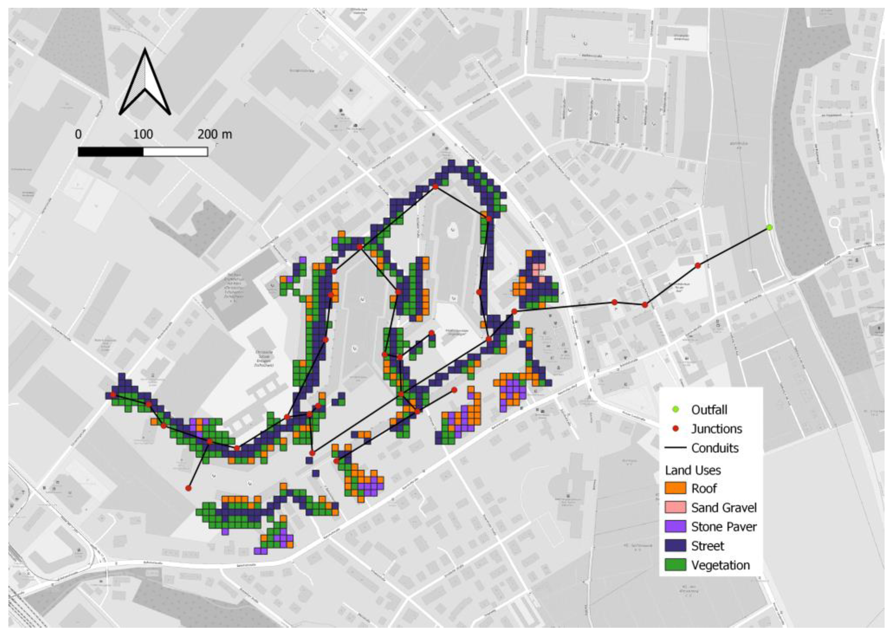
An urban catchment in Dresden, the capital of Saxony, eastern Germany was used as the study area. The catchment has a total surface of 22.9 ha, and it is comprised of different land uses, such as mixed settlement, residential areas, schools, and vegetated areas. Land cover data were obtained from the European Settlement Map of the Copernicus Project [28]. Approximately 42.7% of the total catchment area corresponds to impervious surfaces, mainly buildings, streets, and parking lots. The rest of the catchment, i.e., 57.3%, corresponds to vegetated surfaces, such as gardens, lawns, and other pervious surfaces. The climate in Dresden is classified as temperate oceanic climate (Cfb), according to the Köppen Climate Classification [29]. The average annual temperature is 9.4 °C, and the average annual precipitation is 665 mm [30].
The sewer system in the area follows a separate scheme; hence, two different types of sewer subnetworks are present. On the one hand, a sanitary system collects the wastewater generated by the different buildings in the area and transports it to a collector in the north of the area, which further transports it to the wastewater treatment plant. Furthermore, runoff produced in the area is collected by a stormwater system and discharged into a nearby river, called Lockwitzbach. In the present study, only the stormwater system was considered in all analyses. Figure 1 illustrates the different characteristics of the study area and its drainage network.
3. Materials and Methods
3.1. Hydrodynamic Simulation and Flooding
Urban drainage models (UDMs) can reproduce the complex dynamics and processes associated with urban pluvial flooding and provide reliable estimations of their dynamics and magnitude. Furthermore, UDMs can also simulate the effects of different types of SUDS on the water balance and drainage networks. In this context, a hydrodynamic model of the study area was developed and implemented in the EPA Stormwater Management Model (SWMM) [31].
Information regarding the structure and hydraulic properties of the separate system in the area was provided by the local wastewater company Stadtentwässerung Dresden GmbH. An automatic subcatchment generator tool (GisToSWMM) was used to determine and delineate the contributing areas and their connection to the sewer system [32]. As an input, the tool requires information about the sewer network structure, a digital elevation model (DEM), and land cover data. Topographic data were obtained from the state service for geoinformation and geodesy Saxony (Staatsbetrieb Geobasisinformation und Vermessung Sachsen [GeoSN]), while land cover types were obtained and adapted from the European Settlement Map of the Copernicus Project [28].
The model performance and accuracy were assessed by comparing simulation data with observed discharge values in the outlet. Available measured data corresponded to fifteen rain events between October 2017 and April 2018. These corresponded to precipitation events with depths above 5 mm and at least 5 h of dry-weather conditions before and after the events. Three performance indicators were used to evaluate model accuracy: Nash–Sutcliffe efficiency (NSE) [33], peak flow error (PFE) [34] and volumetric efficiency (VE) [33]. The outcomes of these indicated that the developed model performed quite well in general, with most of the NSE values higher than 0.7, and most of the PFE and VE values lower than 0.3. Table 2 summarizes the characteristics of the rain events and the goodness-of-fit results obtained.
As mentioned before, hydrologic–hydrodynamic simulations were used to determine which nodes of the sewer system flooded and their corresponding flood volume. Twelve rainfall scenarios were simulated in EPA SWMM. They corresponded to ‘Euler Type II’ design storms [35] with reference to the precipitation intensities of the city of Dresden, Germany, according to the coordinated storm event intensities [36]. Such synthetic events had a five-minute discretization step and were based on the assumption that the largest instantaneous precipitation depth occurred at the end of the first third of the event duration. The twelve Euler Type II design storms used in this study were a combination of three different durations, 30, 120, and 360 min, and four return periods of 10, 20, 50, and 100 years. Synthetic events were selected instead of real precipitation data in order to preserve the occurrence frequency of flooding events, and hence to systematically analyze the influence of SUDS on the network during such conditions.
3.2. Flooded Area and Depth Definition
Determination of flooded areas and their corresponding flooded water depths was achieved by coupling results obtained in EPA SWMM with a surface diffusive overland flow model proposed by Chen et al. [37]. The hydrodynamic model was used to determine the locations of flooding junctions and the total flooded volume in each of them. This information was then used together with a DEM of the study area as an input in the diffusive overland flow model to simulate surface flow to estimate flood extension and depths. In this approach, every raster cell from the DEM acted as storage. The cells located above a flooding node were considered initial source cells and they were filled with the corresponding flood volume from the hydrodynamic simulation results. Flood water was allocated into adjacent cells only if the elevation of the source cell was higher than the nearby ones, thus resembling gravitational surface flow. Using the distributed water volume and the number of cells flooded with water, a flood depth was calculated. If this depth was higher than a given threshold, the new cells filled with water acted as new source cells. The process continued iteratively until a depth threshold was reached or until no new flooded cells were identified. The result of this process was a raster map with the same resolution as the DEM used as input. The values of each cell in the generated flooded map corresponded to water depths. Based on this, it was possible to analyze the extent of flooded areas and flood depths associated with each flooded node in the study area.
3.3. SUDS Design and Costs Estimation
The typologies included in the study were green roofs (GR), permeable pavements (PP), infiltration trenches (IT), and rain gardens (RG). These were selected since they corresponded to the minimum combination of structures that would allow the inclusion of source treatment, transport, and storage/retention strategies. The design parameters for each typology (Table 3) were defined from a previous study [38], in which the authors defined the optimal parameters from the SWMM LID editor by means of a sensitivity analysis.
Different construction and design manuals were evaluated in order to fix a nominal cost (per area unit) for each typology. Torres et al. [39] reported similar conditions to those in the present study, and therefore similar costs were used. These costs were reported as capital and annual maintenance costs (Table 4). The latest were reported annually as a percentage of the capital cost. For calculating the total cost of the solutions, the net present value was estimated, using 25 years as the life expectancy for the structures.
3.4. Optimization Algorithm and Modes Coupling
As can be seen in Table 1, genetic algorithms (GA) are efficient and easily adapted to this type of problems. Due to this reason, it was decided to implement this algorithm for the present study, using MATLAB [40] as the coding platform. Although it was intended to use different optimization algorithms, i.e., simulated annealing, particle swarm, or other non-traditional optimization methodologies, and compare their computational efficiencies, the high running time was a crucial constraint that did not allow for this. However, it is highly recommendable to use and compare different algorithms and methodologies for future studies.
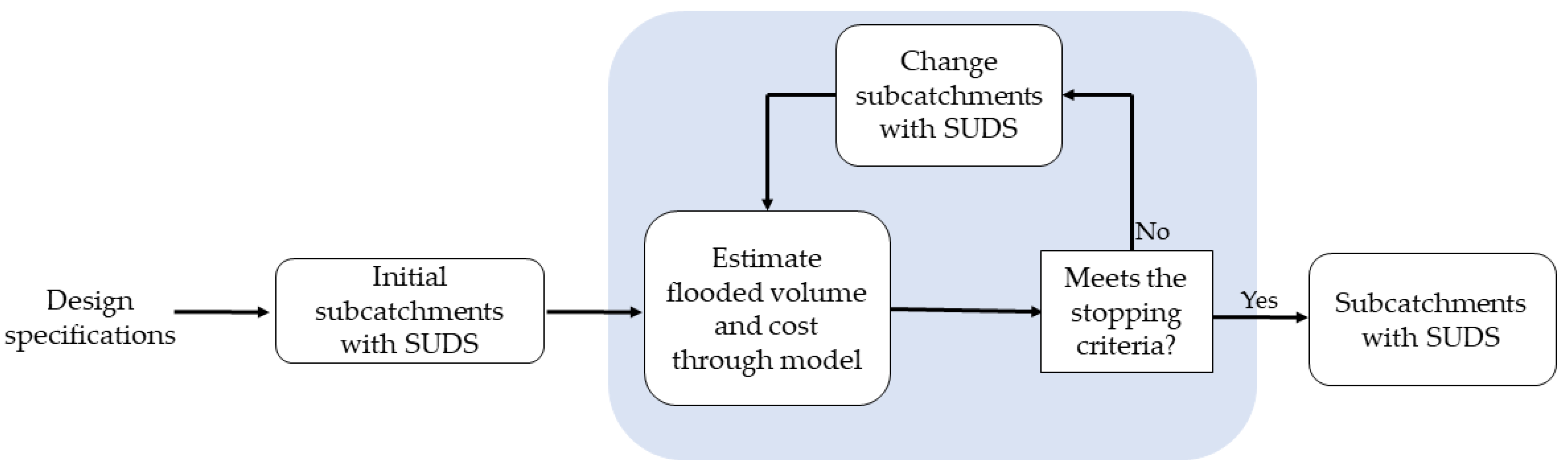
The general framework proposed for the procedure is presented in Figure 2. Regarding the design specifications, the objective functions were defined as total flooded volume and cost of SUDS. At the same time, the independent or decision variables were set as the subcatchments from the EPA SWMM model, which would have the presence of SUDS. The constraints for assigning SUDS were defined depending on the land uses. Hence, typologies were assigned following the description made in Table 5. It is worth clarifying that the presence of SUDS in each subcatchment was defined as total or null, which means that, if a subcatchment was selected, it was assumed that it was completely covered by the corresponding SUDS.
Following the design specifications, the initial configuration was randomly defined by the GA algorithm. After this step, the iterative process (defined as the blue rectangle from Figure 2) started. The total flooded volume (calculated as the sum of the volume flooded in each node) and the costs of the solutions were determined. At each step, the GA automatically defined whether the stopping criteria had been met, defined in MATLAB as: Max_Stall_Generations = 20, and Tol_Fun = 0.001. If the stopping criteria were not met, the algorithm automatically assigned SUDS in different subcatchments, and started the process again. Once the stopping criteria were met, the final design was reached. As this problem consisted of a multi-objective optimization, the final design was a Pareto front, which presented the optimal solutions of SUDS in terms of costs and flooded volume.
The computational complexity of the methodology consisted of interconnecting the different modules/stages of the process. Initially, the UDM developed in SWMM had to be automatically coupled with a Python-based tool to develop, run, and extract the results of the models systematically. With this capability, the next step of the procedure consisted of developing a MATLAB script that processed the results of the UDM and used the extracted results as the objective functions of the GA algorithms. Once the optimal configurations of SUDS were found, another computational resource had to be developed in order to generate the results. On one side, MATLAB was used to develop a script to generate and analyze the Pareto fronts. On the other side, a QGIS-Python script was developed that allowed the mapping of the results, based on the selection of SUDS yielded by the optimization problem. Lastly, each optimal scenario was coupled with the 2D flood propagation model, which generated flood maps using and flood depths. The complete codes are publicly available in the GitHub profile of the first author of this article.
4. Results and Discussion
4.1. Reference Scenarios
The reference scenarios consisted of hydrodynamic and flooding simulations on the study area for the 12 design events, without the presence of SUDS. The results obtained were the total flooded volume, area, and depth for each rainfall event. Results indicated that flooding occurred in all scenarios, but in different amounts, ranging from 471 m3 to 1250 m3 of flooded water (see Table 6). As expected, the return period and the duration of the rainfall events had a strong influence on the generated flood volumes. The increase in these two variables always generated a larger amount of water flooding. Something similar occurred with the maximum flood height, in which the difference among events did not exceed 25 cm.
However, the flooded area did not present the same dynamics. In this case, results were not directly related to the nature of the rainfall events, as the flooded area only varied from 4020 m2 to 4712 m2. These variations were not directly related to the characteristics of the events. The only outlier was the rainfall event with T = 100 years and d = 360 min, where the area flooded reached 6100 m2.
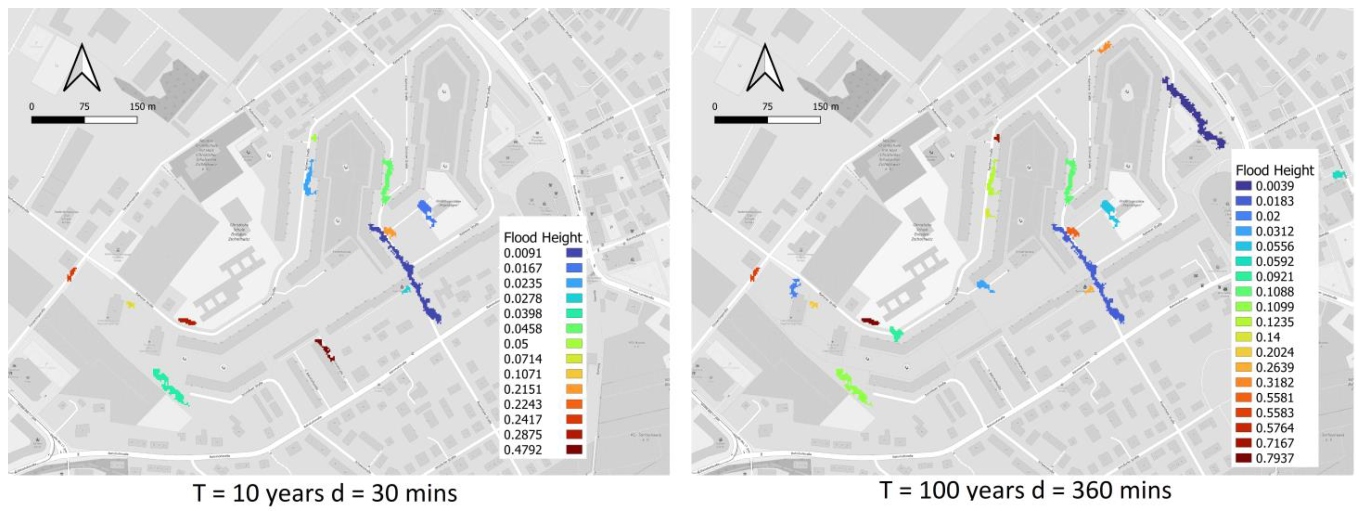
Figure 3 presents the flood maps obtained for the two extreme rain events (lowest and highest rainfall depth). The analysis of these events, which coincided with the dynamics identified for the rest of them, showed that the most susceptible areas to be flooded were the same in all cases. Regarding flood heights, they ranged between 0.009 m and 0.47 m for the smallest event. As the design event was larger, the maximum flood depths increased, and also new flooded areas gradually appeared. The event with the highest flood depths reached values of up to 0.8 m, and presented new flooded areas with higher water levels.
4.2. Pareto Front for SUDS Cost Efficiency
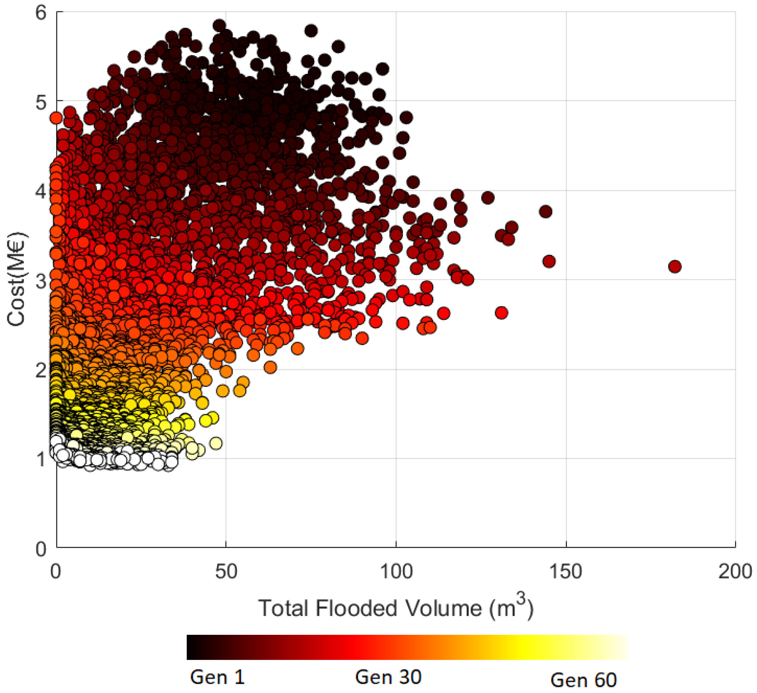
The optimization–selection process was performed 12 times, one for each rainfall design event. Overall, each process took from 6000 to 30,000 iterations, depending on the rain event, which took between 6 and 9 h of computational processing time. Furthermore, the number of generations needed for the GA algorithm to reach the stopping criteria ranged from 20 to 60. To illustrate the performance of the GA algorithm and the improvements reached at each generation, Figure 4 shows the 11,600 iterations that were necessary to reach the Pareto front for the event with T = 10 years and d = 30 min.
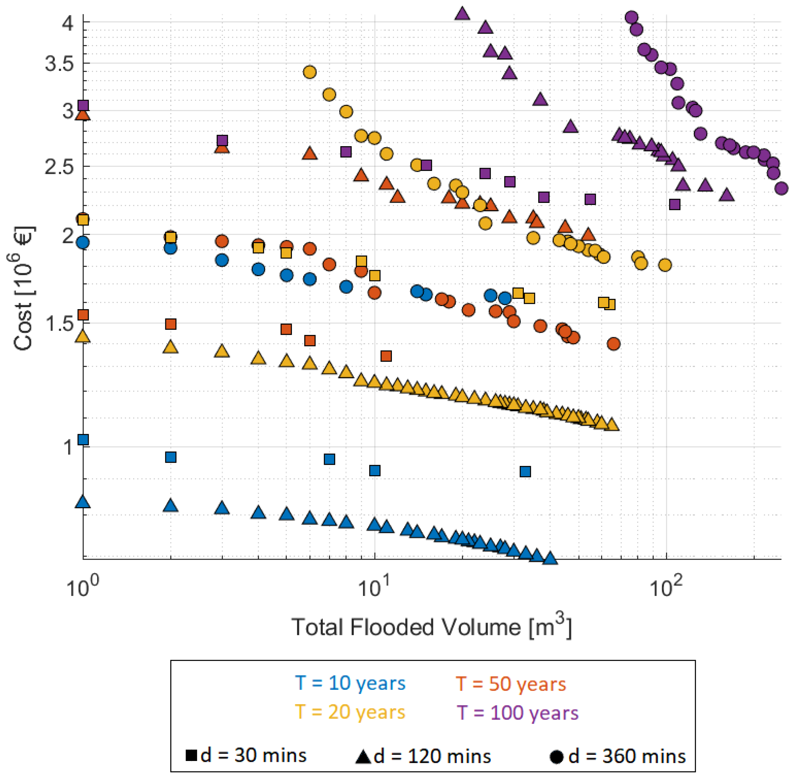
The twelve Pareto fronts were highly variable, depending on the rainfall events (see Figure 5). Overall, it was identified that the larger the event was, the greater the range of variation of costs and flooded volume. From the twelve events, nine offered solutions in which flooding was reduced completely.
Regarding the influence of hydrological variables of rain events, it was not possible to identify a clear pattern. In all cases, the events with the highest costs were the ones with a duration of 360 min. However, for the 10- and 20-year return period events, the 120 min duration event had lower implementation costs. For 50 and 100 years, the 30 min event had the lowest costs. In addition, it was identified that there were events with similar behaviors within them, and in none of these cases were the return period or the duration the same.
To select a specific configuration from each Pareto front, the cost efficiency of each point was calculated, and the one with the highest performance was selected (Table 7). This efficiency was calculated as the percentage of volume reduced with respect to the reference scenario, per million euros invested. Additionally, the total investment for each configuration was included. In this case, the indicator was highly correlated with the return period of the events. The cost efficiency of each scenario reduced progressively when the return period increased. Consequently, these solutions were selected for assessing the effect of SUDS in the flooding areas and depths (Section 4.4). In all cases, it was identified that the process was influenced by the costs of the solutions: the solution with the lowest investment was always the most cost efficient.
4.3. Typologies Selection and Distribution
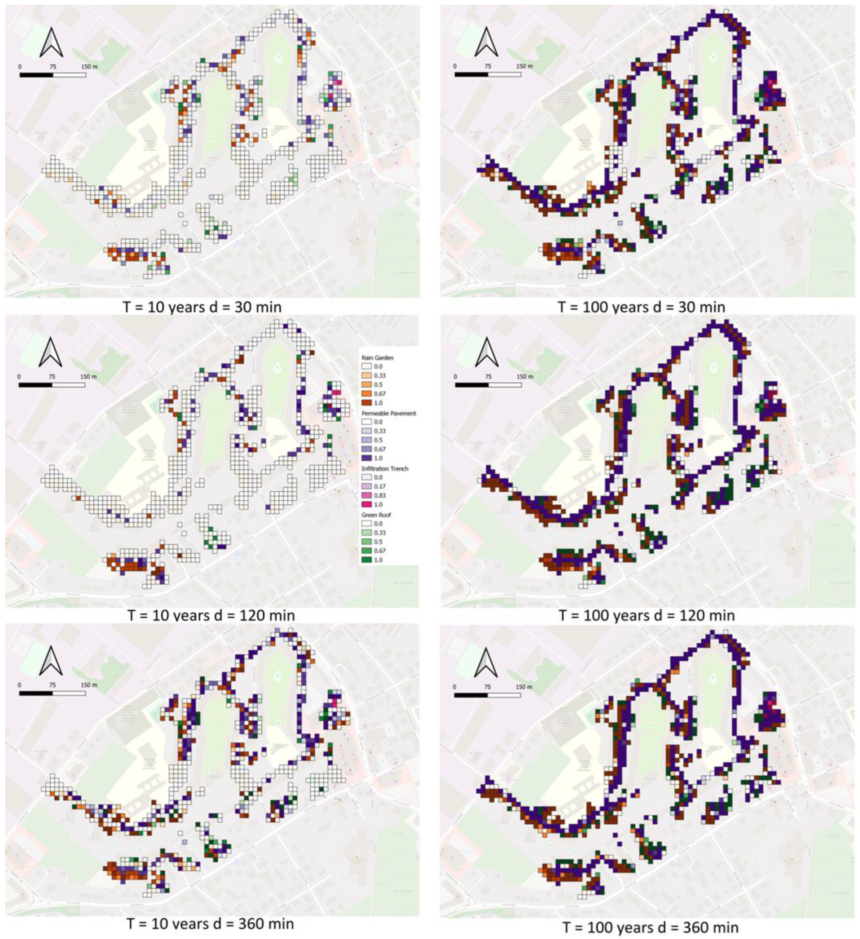
Figure 6 presents the frequency with which each subcatchment was selected for SUDS implementation over the different configurations in the Pareto front. Results are shown only for the two extreme return periods (10 and 100 years). However, the dynamics found for the rest of the events were similar. As expected, results suggested that increasing return periods led to a higher implementation of SUDS. This makes practical sense and is in agreement with previous studies [17,19]. The same dynamics were identified for the duration of the events. These results suggest that the nature of the rainfall design event has a clear effect on SUDS implementation, and it is highly advisable to select an accurate design event from the beginning of the process.
Regarding the spatial distribution of SUDS, in the events with T = 100 years, almost all subcatchments were selected, and their selection frequencies were high (in many cases 1). It was also possible to identify some differences between the three events, with progressive but slight increases in the implementation of SUDS, as the duration of the event increased. On the other hand, for the 10-year return period, it was identified that the differences between the three events were sharper. In all cases, the distribution of SUDS started from focused and specific locations, and as the duration of the event increased, these zones were expanded. These areas coincided with the susceptible areas of flooding from Figure 3, leading to the conclusion that this is an important aspect to consider when placing and designing SUDS.
With respect to the use of typologies, PP were identified as the most used, followed by RG and GR, while IT were rarely used. It was identified that the frequency and distribution of SUDS were directly related to the land uses in the basin. Thus, PP constituted the most used typology due to the fact that the land use suitable for their installation (stone paver and streets) was the most common in the basin. The same occurred with the rest of the typologies. This was evidenced by the clear similarity between the SUDS selection maps and the land-use maps of the case study (Figure 1). From this, it was possible to identify that the selection of SUDS was based primarily on land uses, rather than on the suitability or performance of each typology. No clear pattern was identified regarding how certain typologies were favored depending on the hydrological conditions of the design events.
4.4. Flooded Area and Depth
The analysis of flood areas also identified a differential effect of SUDS depending on the rainfall event (see Table 8). The range of flooded area reduction (with respect to the reference scenario) varied between 0.5% and 40%. When investigating the reasons for such a high range of reductions, it was found that, although the return period and the duration of the events did show some relationship with the results, this dynamic was not conclusive. A tendency was identified showing that the higher the return period, the greater the percentage reduction in the flooded area. However, this did not apply for all return periods (e.g., 10 and 20 years). Likewise, variability in the results was identified within the same return periods, which could be attributed to the effects of the durations of the events. However, this dynamic was not consistent for all durations.
The variables that did have a direct and consistent relationship with the reduction in the flooded area were the total cost of the solution and the flooded area of the reference scenario (presented in Table 7). In both cases, a proportional relationship was identified between the variables and the performance of SUDS. This latest statement leads to the conclusion that when assessing the effectiveness of SUDS mitigating areas flooded, the most relevant variables to consider are the reference area flooded and the money to be invested in the solution.
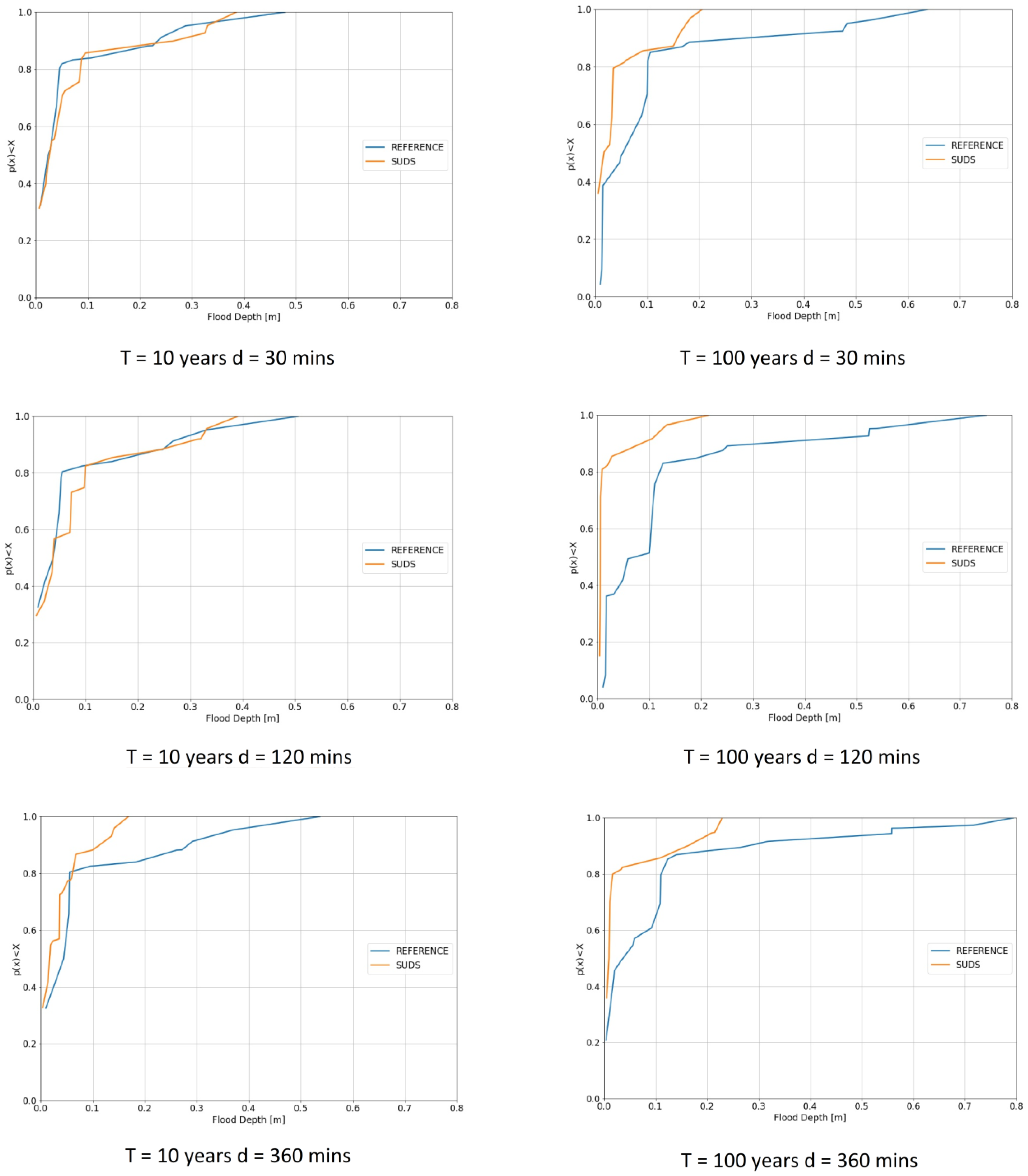
Figure 7 illustrates the effect of SUDS on the flood depths as a function of the return period and the duration of the rain events. The empirical cumulative distributions of flood depths for the reference (i.e., without SUDS implementation) and SUDS scenarios are compared. Only the results for the 10- and 100-year return period scenarios are shown. Regarding the reference conditions, outcomes of this analysis indicate that for all rainfall scenarios, between 85% and 90% of the flooded areas had an associated depth equal to or lower than 0.2 m. Furthermore, maximum flooded depths ranged between 0.4 and 0.8 m, and increased with higher durations and higher return periods, as expected due to the increase in flooded volumes.
The implementation of SUDS led to a general reduction in maximum flooded depths, which ranged between 0.15 and 0.4 m. The results suggest that the efficiency of water depth reduction may have been influenced by the event intensity. In fact, the highest reductions were obtained for the 100-year return period events, where the SUDS implementation led to a decrease in depths from values higher than 0.65 m in the reference conditions to depths lower than 0.25 m. A similar behavior can be seen for the 10-year return period event with the highest duration, i.e., 360 min. However, for the other two scenarios of the 10-year return period, the reduction in maximum flood depths was not as significant as in the other cases.
The reason for this type of behavior may be associated with the optimization algorithm used. The current approach focused on reducing total flood volume, however this does not necessarily imply that flooded areas and depths were proportionally decreased. In some cases, topography does not allow for a wide diffusion of flood water, thus leading to small flooded areas with greater depths. Reducing total flooding volumes in the catchment may then lead to small reductions in flooded areas and depth, since it would focus only on specific parts of the catchment. This can be seen, for example, in the low percentage of reduced flooded areas in most of the scenarios (see Table 8) and the low depth reductions in scenarios 10T_30D and 10T_120D. For events with a higher intensity and duration, in which total flood was influenced by more than one overflowing node, more SUDS were allocated in the catchment, and the reduction in flooded areas and depths were higher, as can be seen in the results obtained in Table 8 and Figure 7. Further developments of the approach could be focused on using flooded areas or depths as additional objectives of the optimization algorithm.
4.5. Combined Frequencies Analysis
The final step of the study consisted of generating a combined scenario (Figure 8) by calculating the cumulative frequency of selection of the subcatchments, calculated as the normalized sum of the 12 independent scenarios. This final scenario was performed in order to provide a final recommendation for SUDS implementation in the area considering all the 12 rainfall events. Results showed that certain subcatchments were selected in 83% of the cases for RG, PP, and GR. At the same time, the maximum frequency of selection for IT was 65%.
The results suggest that the most relevant variable in the process was the spatial distribution of floods. This is evidenced by the high correlation between the flood map (Figure 3) and the cumulative frequency map (Figure 8). The area most susceptible to flooding, and therefore the most recommended for implementing SUDS, was the southwestern portion of the basin, with cumulative SUDS implementation frequencies of 0.83. Furthermore, there were zones with intermediate cumulative frequencies (between 0.4 and 0.8), which in all cases were spatially focused. Based on the results obtained, it is suggested that priority should be given to the selection of subcatchments based on the cumulative frequency criteria, but it should also be attempted to cover each of the sensitive areas.
Finally, an analysis was conducted regarding the selection of the different SUDS typologies. As in the individual analyses (of each event), the results suggested that the selection and suitability of the SUDS typologies were due to spatial and land-use criteria, rather than to the inherent characteristics of each typology.
5. Conclusions
The proposed methodology proved to be efficient and applicable to a real case study. The genetic algorithms showed a good performance. However, the running times of the models were high (between 6 and 9 h per scenario). The EPA SWMM hydrodynamic models were successfully coupled to meta-heuristic methodologies, and the flood propagation model allowed successful evaluation of the actual effect of SUDS on flood mitigation. Overall, SUDS showed a high capacity to mitigate flood risk, and in 9 of the 12 scenarios it was possible to find configurations that reduced the flooded volume to 0. The Pareto front results were highly variable depending on the design event used. Consequently, SUDS configurations and their performance also depended highly on the type of event.
Cost efficiency was proposed as a suitable indicator to select configurations within the Pareto front. However, the multiple solutions offered by this type of solution also allowed the inclusion of other selection criteria, such as maximum allowable costs or minimum expected performances. In any case, the proposed methodology seems to be an important asset to assist SUDS decision-making in real case studies.
Regarding the location and frequency of SUDS location, the key aspects identified were the areas susceptible to flooding and the land uses of the basin. Consequently, both the spatial location and the selection of typologies depended more on these aspects than on other possibilities, such as the suitability of the typologies to manage certain rainfall conditions. The cumulative frequency analysis allowed the identification of the most sensitive areas when analyzing the 12 rainfall events. It is suggested that this latest map should be used as the general recommendation for implementing SUDS, as it jointly assesses the effect of SUDS, regardless of the hydrologic characteristics of the rainfall events.
The analysis of flooded areas allowed the identification of a wide range of performances of SUDS, depending on the rainfall event. The investment and the total flooded areas for the reference scenarios were identified as relevant variables when determining these effects. These two variables were even more important than the hydrologic characteristics of the rainfall events.
The analysis of flood depths led to the conclusion that SUDS presented a high potential for reducing the maximum depths. This behavior is clearly correlated with the nature of the rainfall events, as the potential for reduction increased when the return period of the events was higher. As the area and the height of the flooding were identified as key aspects, it is highly recommended to include these variables as part of the objective variables in the optimization algorithm, as it was proven that, for this case, the algorithm prioritized the volume reduction, rather than these two variables.
So far, the existing methodologies and studies in the field had not coupled the optimization algorithms for SUDS selection with a flood propagation model, which is expected to be an important contribution of the present study to the field. Another novel benefit with regard to the methodology proposed was the successful inclusion of different flood indicators, such as flooded volume, depth, and area. Furthermore, it is proposed that selecting SUDS based on the actual suitability of the land uses will strengthen the value of the study. On the other side, there were some limitations regarding the methodology used. First, it is acknowledged that the running time for the optimization algorithms remained very high, and some refinement in this field is still lacking. Secondly, the framework proposed only used four different typologies, and it is still necessary to diversify the number of structures and allow the possibility of interconnecting these structures into treatment trains. Furthermore, an opportunity for future research was identified in the aspect of including climate-change mitigation potential with SUDS. Furthermore, for future studies, it is recommended to evaluate the efficiency of different multi-objective optimization algorithms in order to compare them with GA, and to evaluate the suitability of using a non-parametric test. Additionally, it is suggested to include different objective variables, such as area or flood height. Regarding the cost analysis, it is advisable to include life cost analyses that allow the quantification of the economic benefits obtained due to the reduction in the flood risk by SUDS. Finally, it is necessary to apply the same methodology to different case studies in order to ensure the replicability of the proposed framework.
Author Contributions
Conceptualization, P.F. and J.D.R.-S.; methodology, P.F.; software, P.F.; validation, J.T. and P.K.; formal analysis, P.F.; investigation, P.F.; resources, P.F.; data curation P.F.; writing—original draft preparation, P.F. and J.D.R.-S.; writing—review and editing, P.F.; visualization, P.F.; supervision, J.T. and P.K. All authors have read and agreed to the published version of the manuscript.
Funding
This research was funded by ICETEX, grant number 5334506, granted to the first author. This research was funded by the German Federal Ministry of Education and Research, grant number 01LR2005A.
Institutional Review Board Statement
Not applicable.
Informed Consent Statement
Not applicable.
Data Availability Statement
The scripts and information used are publicly available in the GitHub profile of the first author.
Acknowledgments
The presented work was conducted under the framework of the KlimaKonform project. It is supported by the German Federal Ministry of Education and Research through the funding measure RegIKlim (Regional Information on Climate Action, focus on Model Regions). The KlimaKonform project is a join initiative between the Technische Universität Dresden, the Sächsisches Landesamt für Umwelt, Landwirtschaft und Geologie, the Friedrich-Schiller-Universität Jena, the Helmholtz Zentrum für Umweltforschung and the Leibniz-Institut für ökologische Raumentwicklung e.V. The authors gratefully acknowledge the cooperation with the Stadentwässerung Dresden GmbH.
Conflicts of Interest
The authors declare no conflict of interest.
References
- Arnone, E.; Pumo, D.; Francipane, A.; La Loggia, G.; Noto, L.V. The role of urban growth, climate change, and their interplay in altering runoff extremes. Hydrol. Process. 2018, 32, 1755–1770. [Google Scholar] [CrossRef]
- Zhou, Q. A Review of Sustainable Urban Drainage Systems Considering the Climate Change and Urbanization Impacts. Water 2014, 6, 976–992. [Google Scholar] [CrossRef] [Green Version]
- Ahiablame, L.; Shakya, R. Modeling flood reduction effects of low impact development at a watershed scale. J. Environ. Manag. 2016, 171, 81–91. [Google Scholar] [CrossRef]
- Muthanna, T.M.; Sivertsen, E.; Kliewer, D.; Jotta, L. Coupling Field Observations and Geographical Information System (GIS)-Based Analysis for Improved Sustainable Urban Drainage Systems (SUDS) Performance. Sustainability 2018, 10, 4683. [Google Scholar] [CrossRef] [Green Version]
- Ferrans, P.; Torres, M.N.; Temprano, J.; Sánchez, J.P.R. Sustainable Urban Drainage System (SUDS) modeling supporting decision-making: A systematic quantitative review. Sci. Total. Environ. 2021, 806, 150447. [Google Scholar] [CrossRef]
- Lerer, S.M.; Arnbjerg-Nielsen, K.; Mikkelsen, P.S. A Mapping of Tools for Informing Water Sensitive Urban Design Planning Decisions—Questions, Aspects and Context Sensitivity. Water 2015, 7, 993–1012. [Google Scholar] [CrossRef] [Green Version]
- Torres, M.N.; Sánchez, J.R.; Leitão, J.P.; de Oliveira Nascimento, N.; Granceri, M. Decision support tools for sustainable urban drainage systems: A systematic quantitative review. In Proceedings of the 9th International Conference on Planning and Technologies for Sustainable Management of Water in the City, Lyon, France, 28 June 2016. [Google Scholar]
- Zhang, K.; Chui, T.F.M.; Yang, Y. Simulating the hydrological performance of low impact development in shallow groundwater via a modified SWMM. J. Hydrol. 2018, 566, 313–331. [Google Scholar] [CrossRef]
- Yazdi, J.; Mohammadiun, S.; Sadiq, R.; Neyshabouri, S.S.; Gharahbagh, A.A. Assessment of different MOEAs for rehabilitation evaluation of Urban Stormwater Drainage Systems—Case study: Eastern catchment of Tehran. J. Hydro-Environ. Res. 2018, 21, 76–85. [Google Scholar] [CrossRef]
- Eckart, K.; McPhee, Z.; Bolisetti, T. Multiobjective optimization of low impact development stormwater controls. J. Hydrol. 2018, 562, 564–576. [Google Scholar] [CrossRef]
- Wang, Q.; Zhou, Q.; Lei, X.; Savić, D.A. Comparison of Multiobjective Optimization Methods Applied to Urban Drainage Adaptation Problems. J. Water Resour. Plan. Manag. 2018, 144, 4018070. [Google Scholar] [CrossRef]
- Baek, S.-S.; Choi, D.-H.; Jung, J.-W.; Lee, H.-J.; Lee, H.; Yoon, K.-S.; Cho, K.H. Optimizing low impact development (LID) for stormwater runoff treatment in urban area, Korea: Experimental and modeling approach. Water Res. 2016, 86, 122–131. [Google Scholar] [CrossRef]
- Yang, Y.; Chui, T.F.M. Optimizing surface and contributing areas of bioretention cells for stormwater runoff quality and quantity management. J. Environ. Manag. 2018, 206, 1090–1103. [Google Scholar] [CrossRef]
- Behroozi, A.; Niksokhan, M.H.; Nazariha, M. Developing a simulation-optimisation model for quantitative and qualitative control of urban run-off using best management practices. J. Flood Risk Manag. 2015, 11, S340–S351. [Google Scholar] [CrossRef]
- Huang, C.-L.; Hsu, N.-S.; Liu, H.-J.; Huang, Y.-H. Optimization of low impact development layout designs for megacity flood mitigation. J. Hydrol. 2018, 564, 542–558. [Google Scholar] [CrossRef]
- She, L.; Wei, M.; You, X.-Y. Multi-objective layout optimization for sponge city by annealing algorithm and its environmental benefits analysis. Sustain. Cities Soc. 2021, 66, 102706. [Google Scholar] [CrossRef]
- Bakhshipour, A.E.; Dittmer, U.; Haghighi, A.; Nowak, W. Toward Sustainable Urban Drainage Infrastructure Planning: A Combined Multiobjective Optimization and Multicriteria Decision-Making Platform. J. Water Resour. Plan. Manag. 2021, 147, 04021049. [Google Scholar] [CrossRef]
- Lopes, M.D.; da Silva, G.B.L. An efficient simulation-optimization approach based on genetic algorithms and hydrologic modeling to assist in identifying optimal low impact development designs. Landsc. Urban Plan. 2021, 216, 104251. [Google Scholar] [CrossRef]
- Rezaei, A.R.; Ismail, Z.; Niksokhan, M.H.; Dayarian, M.A.; Ramli, A.H.; Yusoff, S. Optimal implementation of low impact development for urban stormwater quantity and quality control using multi-objective optimization. Environ. Monit. Assess. 2021, 193, 241. [Google Scholar] [CrossRef]
- Men, H.; Lu, H.; Jiang, W.; Xu, D. Mathematical Optimization Method of Low-Impact Development Layout in the Sponge City. Math. Probl. Eng. 2020, 2020, 6734081. [Google Scholar] [CrossRef]
- Tavakol-Davani, H.E.; Tavakol-Davani, H.; Burian, S.J.; McPherson, B.J.; Barber, M.E. Green infrastructure optimization to achieve pre-development conditions of a semiarid urban catchment. Environ. Sci. Water Res. Technol. 2019, 5, 1157–1171. [Google Scholar] [CrossRef]
- Bahrami, M.; Bozorg-Haddad, O.; Loáiciga, H.A. Optimizing stormwater low-impact development strategies in an urban watershed considering sensitivity and uncertainty. Environ. Monit. Assess. 2019, 191, 14. [Google Scholar] [CrossRef] [PubMed]
- Li, J. A data-driven improved fuzzy logic control optimization-simulation tool for reducing flooding volume at downstream urban drainage systems. Sci. Total. Environ. 2020, 732, 138931. [Google Scholar] [CrossRef] [PubMed]
- Chui, T.F.M.; Liu, X.; Zhan, W. Assessing cost-effectiveness of specific LID practice designs in response to large storm events. J. Hydrol. 2015, 533, 353–364. [Google Scholar] [CrossRef]
- Ghodsi, S.H.; Zahmatkesh, Z.; Goharian, E.; Kerachian, R.; Zhu, Z. Optimal design of low impact development practices in response to climate change. J. Hydrol. 2019, 580, 124266. [Google Scholar] [CrossRef]
- Kumar, S.; Guntu, R.K.; Agarwal, A.; Villuri, V.G.K.; Pasupuleti, S.; Kaushal, D.R.; Gosian, A.K.; Bronstert, A. Multi-objective optimization for stormwater management by green-roofs and infiltration trenches to reduce urban flooding in central Delhi. J. Hydrol. 2022, 606, 127455. [Google Scholar] [CrossRef]
- Lu, W.; Qin, X. An Integrated Fuzzy Simulation-Optimization Model for Supporting Low Impact Development Design under Uncertainty. Water Resour. Manag. 2019, 33, 4351–4365. [Google Scholar] [CrossRef]
- JRC. The European Settlement Map 2017 Release; Methodology and Outputof the European Settlement Map (ESM2p5m); European Comission: Brussels, Belgium, 2017; 2p.
- Mindat.org. The Köppen Climate Classification. 2022. Available online: https://www.mindat.org/climate.php (accessed on 15 January 2023).
- DWD. Deutsche Wetter Dienst. 2022. Available online: https://www.dwd.de/DE/wetter/wetterundklima_vorort/sachsen/dresden/_node.html (accessed on 15 January 2023).
- Rossman, L. Storm Water Management Model Users Manual Version 5.1; US EPA Office of Research and Development; EPA: Washington, DC, USA, 2015.
- Warsta, L.; Niemi, T.J.; Taka, M.; Krebs, G.; Haahti, K.; Koivusalo, H.; Kokkonen, T. Development and application of an automated subcatchment generator for SWMM using open data. Urban Water J. 2017, 14, 954–963. [Google Scholar] [CrossRef]
- Criss, R.E.; Winston, W.E. Do Nash values have value? Discussion and alternate proposals. Hydrol. Process. 2008, 22, 2723–2725. [Google Scholar] [CrossRef]
- Kim, Y.; Chung, E.-S.; Won, K.; Gil, K. Robust Parameter Estimation Framework of a Rainfall-Runoff Model Using Pareto Optimum and Minimax Regret Approach. Water 2015, 7, 1246–1263. [Google Scholar] [CrossRef]
- DWA-A118; Abwasser und Abfall e.V. DWA Deutsche Vereinigung fur Wasserwirtschaft.Arbeitsblatt DWA-A 118 Hydraulische Bemessungund Nachweis Hydraulische Bemessung und Nachweis. Abwasser und Abfall e.V. DWA Deutsche Vereinigung fur Wasserwirtschaft: Hennef, Germany, 2006.
- Junghaenel, T.; Ertel, H.; Deutschländer, T. Bericht zur Revision der Koordinierten Starkregen Regionalisierung und -Auswertung des Deutschen Wetterdienstes in der Version; German Meteorological Service: Offenbach am Main, Germany, 2010.
- Chen, W.; Huang, G.; Zhang, H. Urban stormwater inundation simulation based on SWMM and diffusive overland-flow model. Water Sci. Technol. 2017, 76, 3392–3403. [Google Scholar] [CrossRef]
- Ferrans, P.; Temprano, J. Continuous Quantity and Quality Modeling for Assessing the Effect of SUDS: Application on a Conceptual Urban Drainage Basin. Environ. Process. 2022, 9, 58. [Google Scholar] [CrossRef]
- Torres, A.M. E2STORMED decision support tool guidelines. 2015. [Google Scholar]
- Matlab. 2022. Available online: https://es.mathworks.com/products/matlab.html (accessed on 15 January 2023).
Figure 1.
Case Study Area representing land uses and drainage network.

Figure 2.
Optimization framework for SUDS definition.

Figure 3.
Reference scenario flood map for the two extreme events.

Figure 4.
Pareto front with generations history for rainfall event T = 10 years and d = 30 min.

Figure 5.
Pareto front for volume reduction vs. costs for SUDS optimization process in 12 different rainfall design events. Color scale for different return periods, and marker shapes for the duration of the events.
Figure 5.
Pareto front for volume reduction vs. costs for SUDS optimization process in 12 different rainfall design events. Color scale for different return periods, and marker shapes for the duration of the events.

Figure 6.
SUDS frequency selection in the Pareto front solutions for events.

Figure 7.
Cumulative density probability curve of flood depths for reference and SUDS scenarios in 6 rainfall events.
Figure 7.
Cumulative density probability curve of flood depths for reference and SUDS scenarios in 6 rainfall events.

Figure 8.
Combined scenario of subcatchment selection for SUDS implementation.

Table 2.
Rain characteristics and goodness-of-fit results.
| Event | Depth [mm] | Duration [h] | Return Period [Years] | NSE | PFE | VE |
|---|---|---|---|---|---|---|
| 1 | 5.8 | 220 | 0.16 | 0.72 | 0.07 | 0.02 |
| 2 | 6 | 255 | 0.16 | 0.87 | 0.23 | 0.28 |
| 3 | 5.3 | 240 | 0.13 | 0.77 | 0.30 | 0.30 |
| 4 | 10.6 | 235 | 0.50 | 0.95 | 0.03 | 0.07 |
| 5 | 5.9 | 150 | 0.17 | 0.95 | 0.30 | 0.04 |
| 6 | 9.5 | 245 | 0.39 | 0.55 | 0.24 | 0.20 |
| 7 | 11.8 | 365 | 0.62 | 0.87 | 0.25 | 0.17 |
| 8 | 9 | 305 | 0.35 | 0.78 | 0.28 | 0.22 |
| 9 | 5.4 | 220 | 0.14 | 0.49 | 0.08 | 0.48 |
| 10 | 6.9 | 335 | 0.21 | 0.78 | 0.33 | 0.03 |
| 11 | 7.5 | 195 | 0.25 | 0.87 | 0.29 | 0.05 |
| 12 | 9.9 | 380 | 0.42 | 0.74 | 0.00 | 0.12 |
| 13 | 5.1 | 205 | 0.13 | 0.69 | 0.60 | 0.08 |
| 14 | 22.1 | 670 | 3.15 | 0.84 | 0.36 | 0.24 |
| 15 | 5.7 | 70 | 0.17 | 0.70 | 0.26 | 0.09 |
Table 3.
Design parameters used in the EPA SWMM LID editor for green roofs (GR), rain gardens (RG), infiltration trenches (IT, and permeable pavements (PP).
Table 3.
Design parameters used in the EPA SWMM LID editor for green roofs (GR), rain gardens (RG), infiltration trenches (IT, and permeable pavements (PP).
| Variable | Units | GR | RG | IT | PP |
|---|---|---|---|---|---|
| Surface | |||||
| Berm Height | mm | 90.00 | 150.00 | 0.00 | 0.00 |
| Vegetation volume | mm | 0.10 | 0.00 | ||
| n Manning | mm | 0.09 | 0.11 | 0.24 | 0.03 |
| Slope | % | 1.00 | 1.00 | 1.00 | 1.00 |
| Soil | |||||
| Thickness | mm | 30.00 | 500.00 | 150.00 | |
| Porosity | % | 0.47 | 0.40 | 0.43 | |
| Field capacity | % | 0.24 | 0.17 | 0.10 | |
| Wilting point | % | 0.07 | 0.11 | 0.02 | |
| Conductivity | mm/h | 265.67 | 167.99 | 115.00 | |
| Conductivity slope | - | 10.00 | 21.09 | 10.00 | |
| Suction head | mm/h | 65.00 | 37.31 | 65.00 | |
| Storage | |||||
| Thickness | mm | 200.00 | 500.00 | 10.00 | |
| Void ratio | % | 0.58 | 0.75 | 0.54 | |
| Seepage rate | mm/h | 101.10 | 24.00 | 172.00 | |
| Drain | |||||
| Flow coefficient | - | 2.00 | 2.00 | ||
| Flow exponent | - | 0.50 | 0.50 | ||
| Offset | mm | 0.00 | 0.00 | ||
| Pavement | |||||
| Thickness | mm | 50.00 | |||
| Void ratio | % | 0.37 | |||
| Impervious surface fraction | % | 0.08 | |||
| Permeability | mm/h | 745.33 | |||
| Drainage Mat (Green Roofs) | |||||
| Thickness | mm | 10.00 | |||
| Void fraction | % | 0.47 | |||
| n Manning | mm | 0.07 | |||
Table 4.
Capital and annual maintenance costs for SUDS.
| Typology | Capital Cost [€/m2] | Annual Maintenance Cost [%/m2-Year] |
|---|---|---|
| GR | 145 | 10 |
| RG | 50 | 5 |
| IT | 120 | 2.5 |
| PP | 60 | 0.1 |
Table 5.
Typologies assigned by land use.
| Land Use | Typology Assigned |
|---|---|
| Stone paver | Permeable pavement |
| Vegetation | Rain garden |
| Roof | Green roof |
| Street | Permeable pavement |
| Sand gravel | Infiltration trench |
Table 6.
Flooded volume, area, and height for the reference scenarios.
| R. Period [Years] | Duration [Mins] | Flooded Volume [m3] | Flooded Area [m2] | Maximum Flooded Height [m] |
|---|---|---|---|---|
| 10 | 30 | 471 | 4172 | 0.48 |
| 10 | 120 | 526 | 4420 | 0.51 |
| 10 | 360 | 565 | 4020 | 0.54 |
| 20 | 30 | 612 | 4048 | 0.59 |
| 20 | 120 | 688 | 4212 | 0.64 |
| 20 | 360 | 724 | 4236 | 0.66 |
| 50 | 30 | 813 | 4236 | 0.76 |
| 50 | 120 | 937 | 4564 | 0.83 |
| 50 | 360 | 987 | 4480 | 0.66 |
| 100 | 30 | 978 | 4488 | 0.64 |
| 100 | 120 | 1182 | 4712 | 0.75 |
| 100 | 360 | 1250 | 6100 | 0.79 |
Table 7.
Cost efficiency for the 12 rainfall events.
| R. Period [Years] | Duration [Mins] | Total Investment [106 €] | Cost Efficiency of Selected Configuration [% Volume Reduced/106 €] |
|---|---|---|---|
| 10 | 30 | 0.92 | 1.06 |
| 10 | 120 | 0.69 | 1.34 |
| 10 | 360 | 1.64 | 0.59 |
| 20 | 30 | 1.35 | 0.73 |
| 20 | 120 | 1.99 | 0.46 |
| 20 | 360 | 1.43 | 0.65 |
| 50 | 30 | 1.62 | 0.59 |
| 50 | 120 | 1.08 | 0.87 |
| 50 | 360 | 1.86 | 0.50 |
| 100 | 30 | 2.26 | 0.43 |
| 100 | 120 | 2.34 | 0.39 |
| 100 | 360 | 2.32 | 0.34 |
Table 8.
Reference areas flooded and SUDS performance reducing these areas.
| R. Period [Years] | Duration [Mins] | Total Investment [106 €] | Reference Flooded Area [m2] | SUDS Flooded Area [m2] | Reduction Area Flooded [%] |
|---|---|---|---|---|---|
| 10 | 30 | 0.92 | 4172 | 4020 | 3.64 |
| 10 | 120 | 0.69 | 4420 | 4020 | 9.05 |
| 10 | 360 | 1.64 | 4020 | 4000 | 0.50 |
| 20 | 30 | 1.35 | 4048 | 4040 | 0.20 |
| 20 | 120 | 1.99 | 4212 | 3936 | 6.55 |
| 20 | 360 | 1.43 | 4236 | 3972 | 6.23 |
| 50 | 30 | 1.62 | 4236 | 3960 | 6.52 |
| 50 | 120 | 1.08 | 4564 | 4480 | 1.84 |
| 50 | 360 | 1.86 | 4480 | 2896 | 35.36 |
| 100 | 30 | 2.26 | 4488 | 3636 | 18.98 |
| 100 | 120 | 2.34 | 4712 | 3464 | 26.49 |
| 100 | 360 | 2.32 | 6100 | 3656 | 40.07 |
Disclaimer/Publisher’s Note: The statements, opinions and data contained in all publications are solely those of the individual author(s) and contributor(s) and not of MDPI and/or the editor(s). MDPI and/or the editor(s) disclaim responsibility for any injury to people or property resulting from any ideas, methods, instructions or products referred to in the content. |
© 2023 by the authors. Licensee MDPI, Basel, Switzerland. This article is an open access article distributed under the terms and conditions of the Creative Commons Attribution (CC BY) license (https://creativecommons.org/licenses/by/4.0/).
Share and Cite
MDPI and ACS Style
Ferrans, P.; Reyes-Silva, J.D.; Krebs, P.; Temprano, J. Flood Management with SUDS: A Simulation–Optimization Framework. Water 2023, 15, 426. https://doi.org/10.3390/w15030426
AMA Style
Ferrans P, Reyes-Silva JD, Krebs P, Temprano J. Flood Management with SUDS: A Simulation–Optimization Framework. Water. 2023; 15(3):426. https://doi.org/10.3390/w15030426
Chicago/Turabian StyleFerrans, Pascual, Julian David Reyes-Silva, Peter Krebs, and Javier Temprano. 2023. "Flood Management with SUDS: A Simulation–Optimization Framework" Water 15, no. 3: 426. https://doi.org/10.3390/w15030426
Note that from the first issue of 2016, this journal uses article numbers instead of page numbers. See further details here.