
Hydraulic Geometry and Theory of Equilibrium Water Depth of Branching River


1
School of Marine Engineering Equipment, Zhejiang Ocean University, Zhoushan 316022, China
2
School of Naval Architecture and Maritime, Zhejiang Ocean University, Zhoushan 316022, China
*
Author to whom correspondence should be addressed.
Water 2023, 15(3), 430; https://doi.org/10.3390/w15030430
Submission received: 24 October 2022
/
Revised: 29 December 2022
/
Accepted: 17 January 2023
/
Published: 20 January 2023
(This article belongs to the Special Issue Hydraulics and Hydrodynamics of Overland Flow—Catchment, Subcatchment, Plot Scale and Experimental Approach)
Abstract
:Based on the flow continuity formula, resistance formula, sediment transport capacity formula and width-depth ratio relationship, the hydraulic geometry relationship and theory of equilibrium water depth for a branching river are established and are suitable for arbitrary section shape. The ratio of cross-sectional area of a distributary channel and the main stream is a power function of its bifurcation ratio with an exponent of 6/7. This was applied to a 12.5 m deep-water channel of the Yangtze River (the North Passage, Fujiangsha Waterway and Shiyezhou Waterway). The reliability of the equilibrium water depth was verified and the construction effect of the channel regulation project was predicted. The results show that the regulation project has achieved certain results on the whole, but some waterways still cannot meet the requirement of 12.5 m navigation depth. It is necessary to adjust the layout of the regulation project and focus on increasing the bifurcation ratio and reducing the flow resistance so as to increase the maximum equilibrium water depth.
1. Introduction
The relationship of hydraulic geometry refers to a functional relationship between channel morphology and the dynamic conditions of water and sediment under certain inflow and sediment and boundary conditions, also known as the river facies relationship. Since 1895, when Kennedy [1] proposed the first empirical formula for the river facies relationship without scouring and silting, many scholars have conducted long-term research on the relationships of hydraulic geometry. The early river facies relationship is basically based on empirical formulas. Researchers pursued empirical verification that these relationships indeed exhibited strong goodness of fit for different physiographic sites and settings [2,3,4,5,6,7,8,9]. Based on the relationship between average flow velocity U and average water depth h, which was proposed by Kennedy, Lacey [10] established equations of wetted perimeter χ, hydraulic radius R, and hydraulic gradient J on flow Q and sediment coefficient f. Since then, Blench [11] further introduced the river bank sediment coefficient fw to supplement the formula. Leopold and Maddock [12] proposed a hydraulic geometry relationship as a power function between width, depth, velocity and flow discharge. They used data from 119 measurement stations in nine different basins of America in their study and indicated that the hydraulic geometry of the channel can be expressed as a function of flow discharge.
However, the dimensions of the early river facies relationship formulas are generally not harmonious [13,14]. Since modern times, the study of the river facies relationship has been greatly improved. Velicanov [15] used the bed-forming discharge Q, hydraulic gradient J and the sediment particle size d50 to represent the three factors of meteorology, topography and geological structure, respectively. Using the dimensional analysis method, the expression of river width and water depth is obtained, which is widely used as after simplification.
Many scholars have also studied the hydraulic geometric relationship of branching rivers. Taylor [16] studied the relationship between the bifurcation ratio and the water depth ratio via flume experiments. Marra [17] conducted an experiment on the near bed flow and surface flow diversion model in river bifurcation. Wang [18] obtained the bed material flux upstream and downstream of the Mississippi Achafaraya River Diversion by estimating the controlled large bifurcations. Ding [19] established a formula for calculating the diversion ratio and sediment ratio of the branch channel and verified it based on the measured water and sediment data of several branches in the middle and lower reaches of the Yangtze River. Xie [20] discussed the relationship between the hydraulic elements of the bifurcated channel and the hydraulic elements of the single section and summarized the formation mechanism and evolution law of the bifurcated channel. Wang [21] and Bolla-Pitaluga [22] studied the equilibrium morphology and stability of the channel through a one-dimensional dynamic geomorphological model. According to the vertical distribution of flow velocity and sediment concentration, Han [23] analyzed the relationship between the diversion ratio and the sediment ratio by introducing the equivalent water depth determined by the diversion ratio of the distributary channel. On this basis, Qin [24] considered the transverse circulation effect, further improved the sediment diversion model and obtained the relationship between the sediment diversion ratio and the topography. The model was applied to the qualitative analysis and verification calculation of the Jingjiang channel and the distributary channels in the middle reaches of the Yangtze River, and the results are in good agreement. Lane [25] obtained the flow pattern of a multi-channel river through a high-precision two-dimensional space model. Neary [26], Barkdoll [27] and Dargahi [28] studied the characteristics of water and sediment movement in the branching estuary using a three-dimensional model. Using the theory of minimum energy consumption, Yan [29] analyzed the hydraulic geometry relationship of the branches of alluvial rivers under the condition of free development or restriction and obtained the calculation formulas of diversion angle and deflection angle. Meselhe‘s [30] analysis focused on the dynamics between the flow and sediment delta interconnected channel networks. Bertoldi [31] studied the equilibrium cross-section shape of the branching river through experimental observation. Tong [32] derived two formulas for calculating the diversion ratio of branching rivers by using the equal sediment concentration method and the momentum balance method and considered the formula based on the momentum balance method more accurate. Based on the theories of minimum energy dissipation theory of fluid movement and river morphodynamics, Yang [33] analyzed the relationship between river island shape coefficient and flow and sediment dynamics under stable equilibrium conditions.
Some researchers proposed two different forms of power law, hydropower station hydraulic geometry (AHG) and downstream hydraulic geometry (DHG), and derived the theoretical expressions of AHG and DHG [34,35,36]. Tran used a process-based morphodynamic model to simulate the evolution of tidal inlets towards equilibrium when subjected to a range of tide and wave conditions. Specific attention was given to the evolution of the cross-sectional area of the inlet channel. [37]. D’Alpaos [38] verified that the P-A relationship is not only applicable to the portal section, but also to any section of the tidal inlet, which can be used to predict the long-term seabed terrain evolution of the tidal inlet. Arkesteijn tried to develop analytical solutions for balanced channel profiles [39]. In this study, the term ‘‘hydraulic geometry’’ refers to downstream hydraulic geometry, and discharge values are denoted by bed-forming discharge.
For the river facies relationship with four unknowns B, H, V and J, a set of simultaneous equations can also be used to solve the hydraulic geometric relationship. Usually, only three equations can be introduced, i.e., the flow continuity formula, the resistance formula and the sediment transport capacity formula. In order to make the equations closed, one more equation is needed. In this paper, the aforementioned empirical relationship of the width–depth ratio is introduced to establish a hydraulic geometry relationship suitable for arbitrary section shape.
2. Methods
2.1. Hydraulic Geometry
The relationship of hydraulic geometry refers to a functional relationship between channel morphology and dynamic conditions of water and sediment under certain inflow and sediment and boundary conditions. As for a branching river, considering that the water depth varies along the river width y direction, while the vertical average velocity varies along the river width direction with the water depth, the two-dimensional continuity equation in the integral form is shown as follows:
where Qi is the bed-forming discharge, Bi is the river width, hi(y) is the water depth, ui(y) is the vertical average velocity, and y represents the lateral direction, that is, the river width direction. The subscript i = 0 represents the main stream, and i = 1, 2 represents a distributary channel, as shown in Figure 1.
Similarly, according to the Chezy formula, the two-dimensional resistance equation in integral form is:
where Ji is the hydraulic gradient and Ci is the dimensionless Chezy coefficient, which reflects the river resistance.
The sediment transport capacity can be calculated by the following formula [40]:
where is the sediment transport capacity by volume, that is, the (equilibrium) suspended sediment concentration, Hi is the average water depth, Ui is the average velocity in section, and k0 is a dimensionless constant.
The ratio of width–depth reflects the change in channel morphology, which can be expressed by the following expression:
where Dm is the average particle size, which reflects the influence of the composition of non-uniform sediment on the cross-section morphology. It is usually assumed that the average particle size Dm and morphological coefficient remain unchanged before and after branching.
Based on the Equations (1)–(4), the relationship of hydraulic geometry for arbitrary section shape can be obtained.
Assume that the cross-section morphology of main stream and distributary channel satisfy a same function:
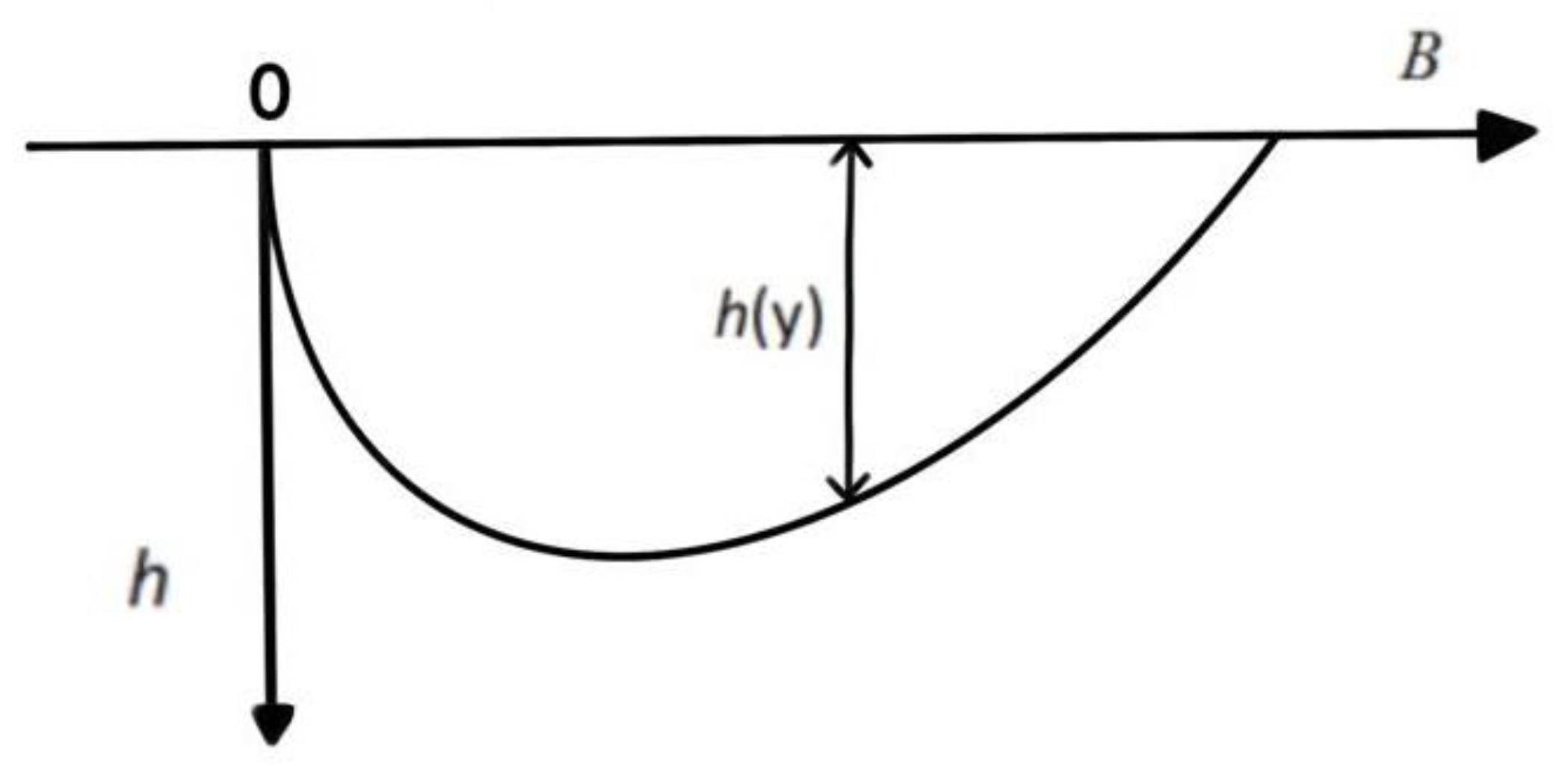
and ; hmax is the maximum water depth in the section, as shown in Figure 2.
Then, the discharge of main stream and distributary channel is:
Let , and
then
k1 is an integral related to the lateral distribution of relative water depth, which can be obtained by numerical integration of terrain curves or calculated using actual terrain data. It is applicable to arbitrary terrain curve, and its value varies with terrain.
Therefore, the bifurcation ratio can be expressed as follows:
The cross-sectional area of the main stream and distributary channel is:
where
k2 is the integral coefficient of the terrain curve, generally between 0.5 and 1. The average velocity of the main stream and distributary channel is:
The average depth of main stream and distributary channel is:
The branch river is in a balanced or quasi-balanced state after long-term dynamic adjustment, and it is generally considered that the sediment transport capacity is the same before and after branching. That is,
According to Equations (3)–(14):
Therefore
Substituting Equation (16) into Equation (9) leads to:
According to Equations (4) and (17), it can be derived:
Equations (19)–(21) are the hydraulic geometry relationship of a branching river, which is suitable for different channel morphology. The ratio of water depth, river width and cross-sectional area of a distributary channel to the main stream is a power function of its bifurcation ratio with exponents of 2/7, 4/7 and 6/7, respectively.
2.2. Theory of Equilibrium Water Depth
For navigable channels, the distribution of equilibrium water depth h(y) along the cross section can be calculated according to Equations (5)–(21):
Equation (22) can be used to calculate the equilibrium water depth.
The equilibrium water depth provides a method to predict the evolution trend of the branch river in addition to the mathematical model and the physical model. It pays more attention to the exploration of the final result, different from the mathematical model, which attaches importance to the process change. For balanced water depth, the mathematical model and physical model have their own advantages and disadvantages.
The flow parameters used in the calculation of equilibrium water depth should be multi-year averages to reflect the equilibrium state of the branching river. However, it is difficult to obtain the measured data of a long river for many years; this is generally calculated using a mathematical model. The upstream boundary condition of the model is the bed-forming discharge, which is calculated using the Makaviev method, and the downstream boundary is the tidal level corresponding to the bed-forming discharge, so as to calculate the flow parameters of the multi-year average value.
When the section shape function is a parabolic curve, that is,
and the integral coefficient of terrain curve k2 = 2/3, then
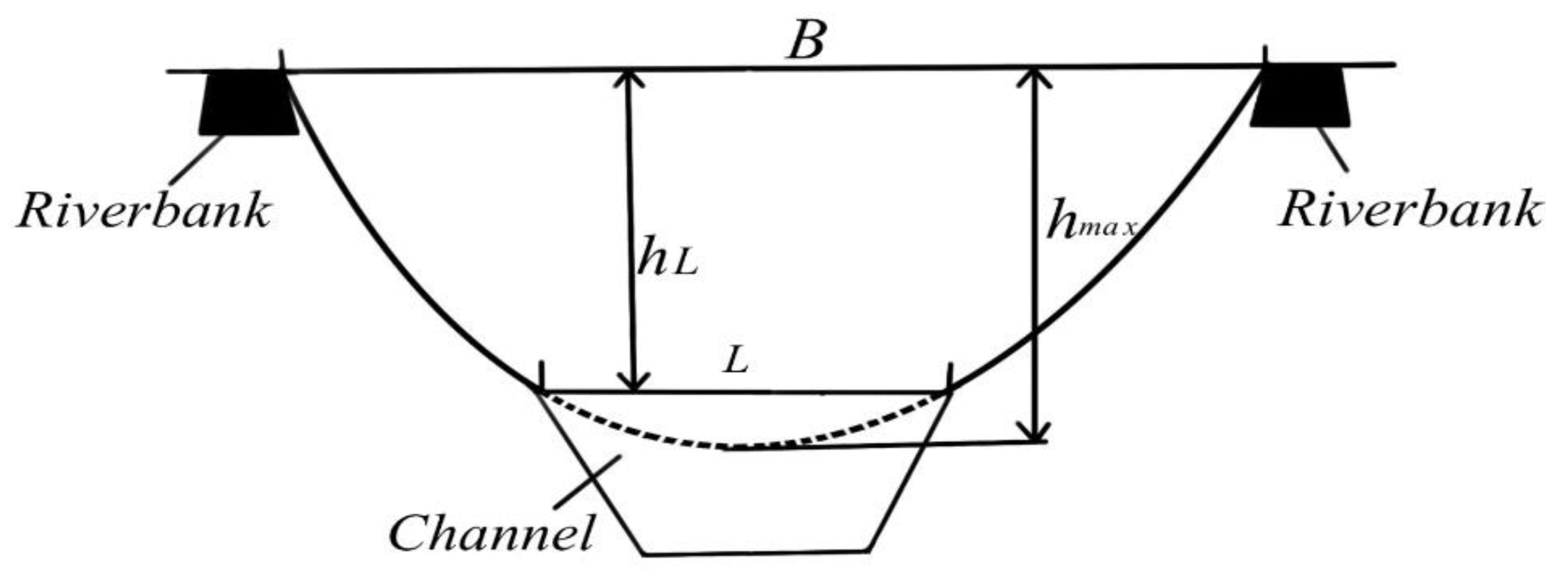
When the channel width is L and the channel is located in the middle of the river (shown in Figure 3), the navigable depth hL within the channel width is:
The difference from the designed navigable depth Hs is:
means the dredging depth required to meet navigation requirements.
When other cross-section shape functions are used, the navigable depth hL can still be calculated according to the channel position by Equation (22).
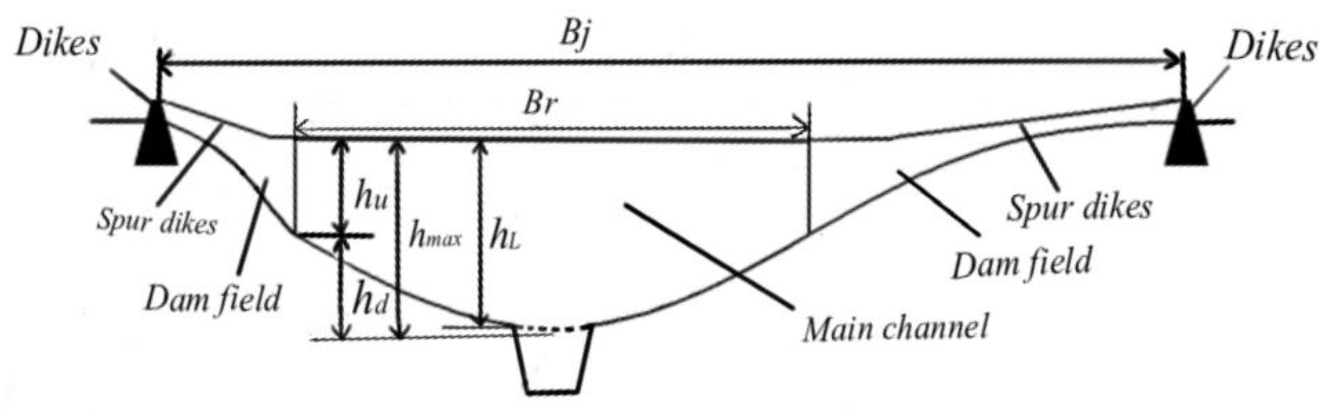
In addition, in waterway regulation and the flood control revetment project, in order to achieve the effect of scouring the riverbed and increasing the water depth of the channel, spur dikes and other regulation buildings are often used to narrow the river channel and flow. The root of the spur dike is generally connected to the river bank or the guide embankment, and the dam head extends to the river center. The line connecting the head of the spur dike group is the regulation line, and the section between the regulation lines is the main channel. Under the action of the spur dike, the flow structures of the main channel and the dam field are quite different. The discharge in main channel is the main factor determining the riverbed topography, and the flow in the dam field has little effect on the riverbed topography.
The average water depth and cross section area of the main channel, which have great influence on navigation, are exactly what we are concerned about. Therefore, the hydraulic geometry of the branching river proposed above should be modified. When there are spur dikes, dikes and other regulation buildings in the branch channel, the hydraulic geometry of the branching river can be changed into the following form:
The cross-section area here only considers the main channel range. The channel section with the spur dike is generalized as shown in Figure 4, and the lower part of the main channel is set to be parabolic.
When Br is the distance between the regulation lines, Bj is the total width, hu is the water depth of the upper rectangular, determined according to the average water depth on the regulation line, and hd is the maximum water depth of lower parabolic, then the main channel section area is:
The equilibrium water depth of the main channel is expressed as:
The maximum equilibrium depth of the main channel hmax is expressed as:
When the channel width is L and the channel is located in the middle of the river, the navigable depth within the channel width is:
When the channel is not in the middle, the navigable depth should be calculated by Equation (30) according to the channel position.
3. Results
The regulation of the Yangtze River deep-water channel project strives to gradually realize the navigation depths of 8.5, 10 and 12.5 m in three phases. In this paper, the equilibrium water depth of the Yangtze River deep-water channel (North Passage, Fujiangsha Waterway and Shiyezhou Waterway) before and after the multi-branch channel project was calculated. The reliability of the equilibrium water depth is verified and the construction effect of the channel regulation project is predicted.
3.1. Equilibrium Water Depth of North Passage
3.1.1. Before the Project
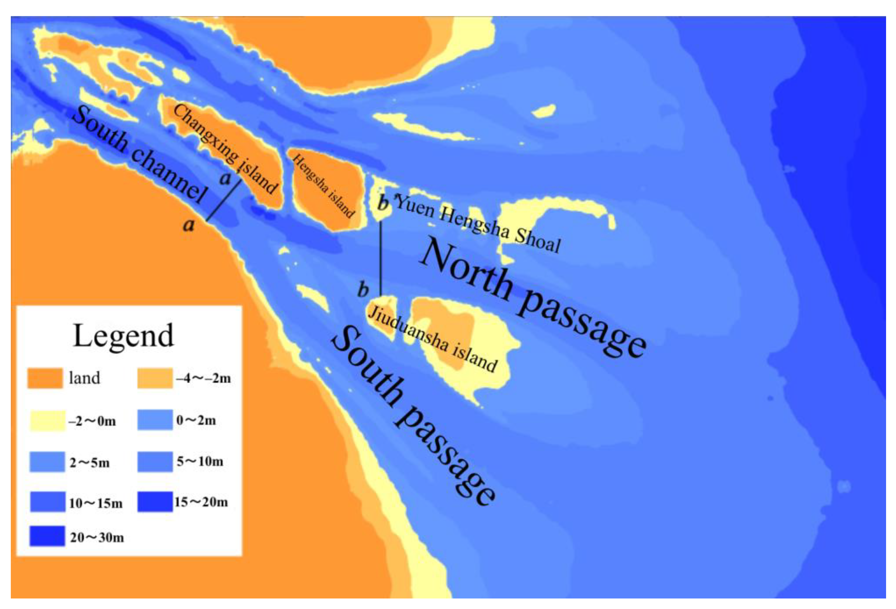
The South Branch of Yangtze Estuary is divided into the South Channel and the North Channel by Changxing Island and Hengsha Island, and the South Channel is divided into the South Passage and North Passage by Jiuduansha. The section a-a’ of the South Channel and the section b-b’ of the North Passage were selected to calculate the maximum equilibrium water depth hmax before the project. The positions of the sections are shown in Figure 5. The shape function of the sections was set as a parabola.
The equilibrium water depth was calculated after obtaining relevant flow parameters from the numerical model. The result is shown in Table 1. The maximum water depth hmax is 6.9 m, which is basically consistent with the actual situation, wherethe water depth at the top of the bar sand section of the Yangtze Estuary channel was maintained at 6–7 m for a long time before the project. This shows that the hydraulic geometry proposed in this paper is suitable for estimating the equilibrium water depth of a branching river.
3.1.2. After the Project
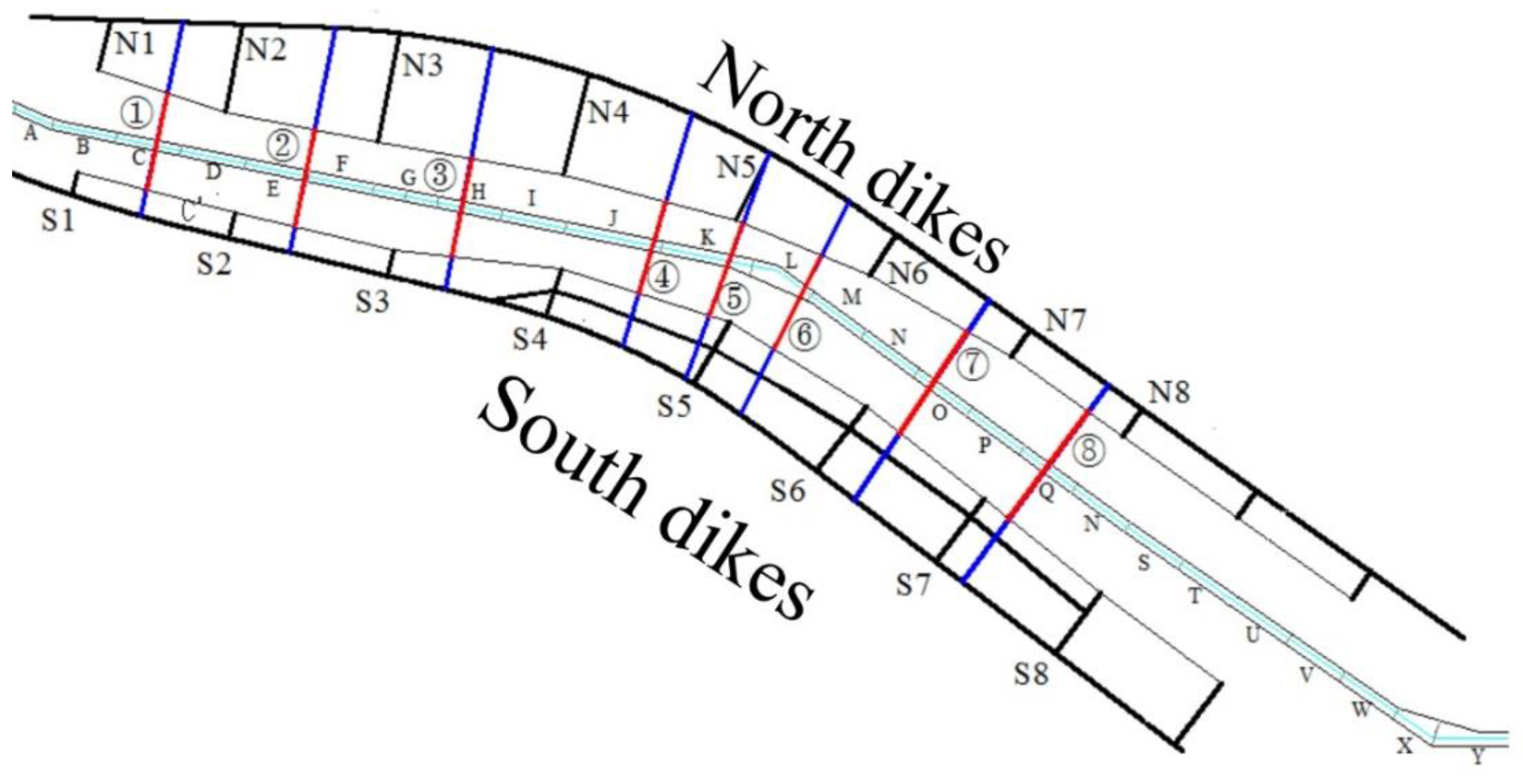
The construction of the North Passage regulation project began in January 1998, and the third phase of the project was completed in March 2010. The north and south guide dikes and spur dikes were built along the shoals on the south and north sides of the North Passage, which significantly changed the hydrodynamics, sediment transport, riverbed topography and cross-section morphology of the North Passage. The target navigation depth is 12.5 m. However, after the third phase of the project, the annual siltation of the channel is still large, and the annual maintenance and dredging volume of the channel is up to 80 million m3. Considering the influence of spur dikes, we used the modified hydraulic geometry relationship to calculate the navigable water depth in the channel. The layout of the regulating structure is shown in Figure 6.
The positions of calculated sections (①~⑧), which are located between spur dikes, are shown in Figure 7.
The navigable water depth calculated according to the hydraulic geometry is shown in Table 2. The navigable water depths in the ①~③ sections of the upper section of the North Passage are 11.46 m, 11.43 m and 11.40 m, respectively, and the difference from the designed water depth is about 1.1 m. The navigable water depths of the ④~⑥ sections of the middle section of the North Passage are 9.66 m, 9.52 m and 9.78 m, respectively, and the difference from the designed water depth is about 2.8 m. The navigable water depths of the ⑦~⑧ sections of the lower section of the North Passage are 10.36 m and 10.39 m, respectively, and the difference from the designed water depth is about 2.1 m. In general, after the third phase of the project, the navigable water depth of the upper section of the North Passage is greater than that of the lower section, and the middle section is the smallest, which is consistent with the actual situation.
The double dikes and spur dikes in the regulation project narrowed the channel. On the one hand, it is beneficial to increase the unit width flow; to a certain extent, it has the effect of beaming water to attack sand and scour the deep channel, which makes the theoretical navigation depth of the North Passage increase obviously, reaching about 10.51 m on average. However, on the other hand, the engineering buildings increase the resistance of the riverbed shape, which reduces the flow. The change of the maximum navigable depth depends on the combined effect of the above two factors. Finally, there is still a gap of about 2 m between the theoretical navigable depth and the designed depth of 12.5 m. This shows that according to the current regulation projects, the navigable depth of 12.5 m cannot be naturally maintained. If the navigable depth of 12.5 m is to be maintained, other regulation projects or a certain amount of dredging is required every year.
3.2. Equilibrium Water Depth of Fujiangsha Waterway
The second phase of the 12.5 m deep-water channel below Nanjing of the Yangtze River mainly extends from Nantong (Tianshenggang) to Nanjing (Xinshengwei) by implementing the regulation project of the key parts of the inner beach of the Yangtze River from Nantong to Nanjing and combining with dredging measures.
3.2.1. Before the Project
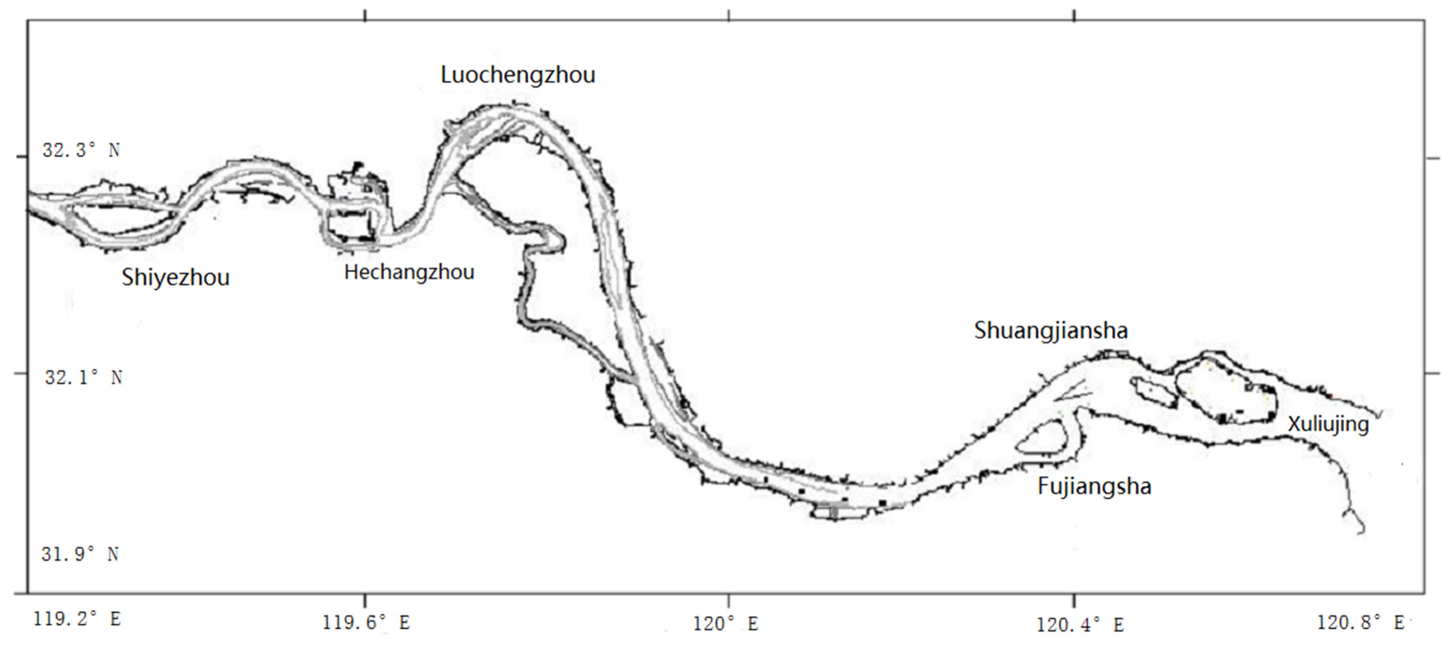
Located between Jiangyin and Jiulonggang, shown in Figure 8, the Fujiangsha Waterway is about 40 km. It is in a pattern of “two-level branching and three-branch coexistence” on the plane. This is the difficulty of the 12.5 m channel regulation below Nanjing and the key control section of the deep-water channel.
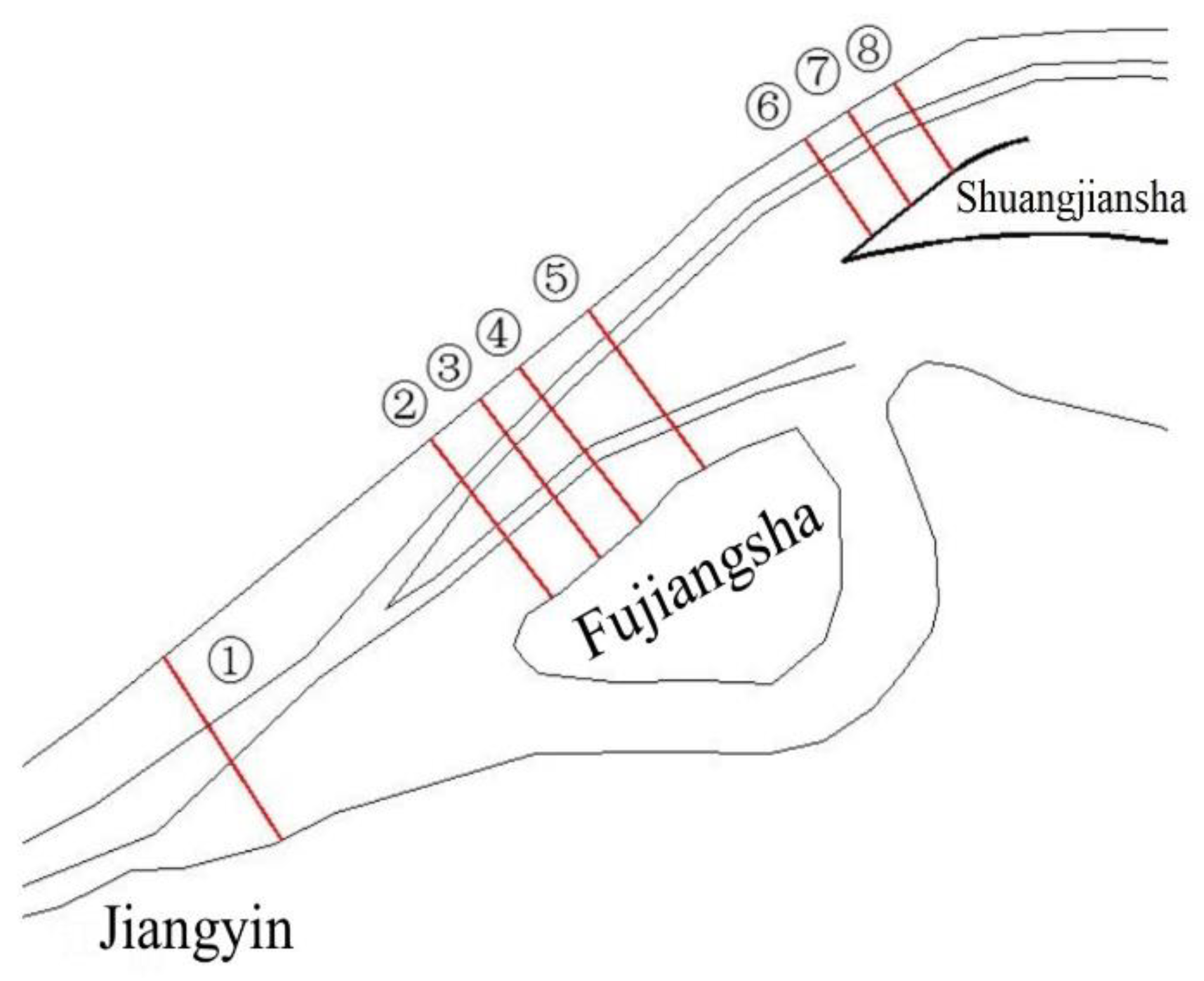
Section ① in the main stream, sections ②~⑤ in the Fujiangsha branch and sections ⑥~⑧ in the Shuangjiansha branch were chosen to calculate the navigable depth hL before the project. The shape function of the sections was set as a parabola. The positions of the sections are shown in Figure 9.
The navigable water depth was calculated after obtaining relevant flow parameters from the numerical model. The results are shown in Table 3.
According to Table 3, the navigable water depth of the Fujiangsha branch is 12.1 m, and the difference from the designed navigable water depth of 12.5 m is about 0.4 m. After proper treatment, it can meet the navigation requirement. The navigable water depth of the Shuangjiansha branch is 7.59 m, and the difference from the designed navigable water depth is 4.91 m. There is a big gap, and it is necessary to carry out large-scale engineering measures to adjust the main stream into the Shuangjiansha branch, so as to realize the design’s navigable water depth of 12.5 m.
3.2.2. After the Project
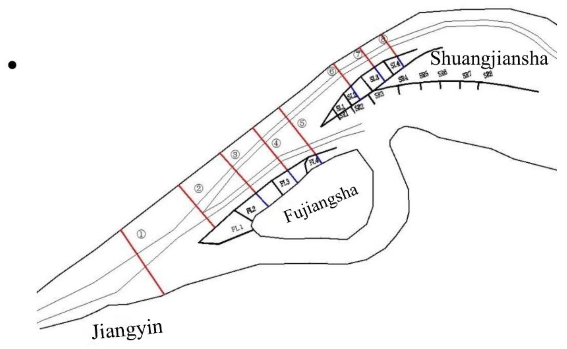
According to the project design, the layout of spur dikes in Fujiangsha and Shuangjiansha branch is shown in Figure 10.
Section ① in the main stream, sections ②~⑤ in the Fujiangsha branch and sections ⑥~⑧ in the Shuangjiansha branch were chosen to calculate the navigable depth hL after the project. Compared with the design navigable depth of 12.5 m, the effect of channel regulation can be predicted and analyzed, which will provide follow-up ideas and scientific basis for channel regulation. The positions of the calculated sections, which are located between spur dikes, are shown in Figure 11.
The navigable water depth calculated according to the hydraulic geometry is shown in Table 4.
The results show that the navigable water depth of the Fujiangsha branch increased from 12.1 m to 13.05 m, which can meet the requirements of the design navigable water depth. However, for the Shuangjiansha branch, although the navigable water depth increased to 10.63 m, it still cannot meet the requirements of the design navigable water depth, which means that there is a certain limit to increasing the equilibrium water depth. The spur dike plays the role of narrowing the river channel, and also leads to increase in the branch resistance and decrease in the bifurcation ratio, which makes the regulation effect fail to achieve the expected goal. Therefore, we should focus on increasing the bifurcation ratio of the channel and reducing the flow resistance to increase the maintainable equilibrium water depth.
3.3. Equilibrium Water Depth of Shiyezhou Waterway
3.3.1. Before the Project
The total length of the Shiyezhou Waterway is about 31 km, shown in Figure 8. Section ① in the main stream and sections ②~⑤ in the Shiyezhou branch were chosen to calculate the navigable depth hL before the project. The shape function of the sections was also set as a parabola. The positions of the sections are shown in Figure 12.
The navigable depth was calculated after obtaining relevant flow parameters from the numerical model. The results are shown in Table 5.
According to the Table 5, the navigable water depth of the Shiyezhou branch is 10.79 m, and the difference from the designed navigable water depth of 12.5 m is about 1.71 m. There is a certain gap, and necessary engineering remediation measures are needed. This shows that according to the current regulation projects, the navigable depth of 12.5 m cannot be naturally maintained. If the navigable depth of 12.5 m is to be maintained, other regulation projects or a certain amount of dredging is required every year.
3.3.2. After the Project
According to the project design, the layout of spur dikes in Shiyezhou Waterway is shown in Figure 13.
Section ① in the main stream and sections ②~⑤ in the Shiyezhou branch were chosen to calculate the navigable depth hL after the project. The positions of the sections are shown in Figure 14. The navigable depth calculated according to the hydraulic geometry is shown in Table 6.
The calculation shows that the navigable water depth of the Shiyezhou branch increased from 10.79 m to 12.95 m, which can meet the requirements of the design navigable water depth. It can be seen that the engineering scheme has a certain regulation effect on the Shiyezhou branch. This shows that according to the current regulation projects, the navigable depth of 12.5 m can be naturally maintained.
4. Discussion
Sediment transport causes riverbed erosion and siltation, which determines the trend of riverbed evolution. When the sediment transport capacity exceeds the sediment concentration, the river channel will be scoured; on the contrary, siltation will occur, which will cause siltation of the channel. Erosion and siltation always exist in natural rivers. If we need to accurately calculate the erosion and siltation of a certain river at a certain time, we can use a mathematical model to calculate it through the difference between the sediment transport capacity and the sediment concentration. However, it is difficult to calculate the water depth of the final form of a river in the future through numerical simulation, because the boundary conditions are always changing. However, this ideal state of balance is also a very interesting and meaningful state. This state is the balance form formed by the long-term dynamic adjustment of the river and the final result of sediment transport. The water depth in this state is the maximum water depth that the channel or river can maintain or reach under certain conditions. Its determination is of great significance for the determination of the design water depth of the channel or the design and implementation of engineering regulation measures.
In the process of establishing our theory and method, we made some assumptions and simplifications, mainly from non-tidal rivers, and assumed a future equilibrium state, in which water depth may approach equilibrium depth. Based on the relevant control equations, the exact relationship between the sections before and after branching under the ideal balance state were obtained. In fact, this is also applicable to tidal rivers and estuaries, just as many relationships applicable to tidal rivers and estuaries were originally derived from flume experiments or non-tidal rivers.
From the results above, we found that the maximum water depth calculated in the North Passage before the project was 6.9 m, which is basically consistent with the actual situation that the water depth at the top of the bar sand section of the Yangtze Estuary channel was maintained at 6–7 m for a long time. Obviously, the results successfully verify the reliability of the proposed method.
The basic reason why this method can be applicable to tidal rivers and estuaries lies in the following two points: Firstly, one of the biggest differences between tidal rivers and estuaries and non-tidal rivers is the change of flow direction, but when we choose a certain time point, this is basically the same as that of non-tidal rivers, that is, it can also conform to our four control equations (Equations (1)–(4)). This is the main reason why this relationship can be also applicable to tidal rivers and estuaries. Secondly, it is obvious that the most critical element in Equation (26) for calculating the equilibrium water depth is the bifurcation ratio before and after branching. In fact, the most important factor here is the ratio of representative discharge before and after branching, rather than a single discharge. Therefore, as long as the corresponding fluctuation flow is selected, the results will be feasible. In this paper, the runoff calculated was used as the representative discharge for non-tidal rivers, the ebb flow calculated was used as the representative discharge for tidal rivers and estuaries, and good results were obtained. This is another important reason why this relationship can be applicable to tidal rivers and estuaries. The calculation of the equilibrium water depth pays more attention to the exploration of the final results, which is different from the characteristics of the mathematical model that pays more attention to the process changes. The impact of scouring and silting changes or sediment transport imbalance in a short period of time on the final results is small and can be ignored to some extent. This provides a method to predict the trend of riverbed evolution in addition to mathematical and physical models that is on a longer time scale. In general, our theoretical derivation method and calculation method of equilibrium water depth are new and unique and are of great convenience and significance in the engineering field.
5. Conclusions
Based on the flow continuity formula, resistance formula, sediment transport capacity formula and width–depth ratio relationship, the hydraulic geometry relationship of a branching river was established that is suitable for arbitrary section shape. The ratio of cross-sectional area of a distributary channel and the main stream is a power function of its bifurcation ratio with an exponent of 6/7. On this basis, the theory of the equilibrium water depth and its calculation method were constructed.
The theory of equilibrium depth provides a method to predict the trend of riverbed evolution in addition to mathematical models and physical models. It pays more attention to the exploration of the final results, which is different from the characteristics of mathematical models that attach importance to process changes. Each has advantages and disadvantages and complements the other.
The theory and calculation method of equilibrium water depth based on hydraulic geometry was applied to the North Passage, Fujiangsha Waterway and Shiyezhou Waterway of Yangtze River. The reliability of equilibrium water depth was verified and the construction effect of the channel regulation project was predicted.
On the one hand, the regulation project is conducive to increasing the unit width flow to a certain extent; it has the effect of water and sand attacking and scouring the deep channel, which increases the equilibrium water depth. On the other hand, the regulation project increases the resistance of the channel, which is not conducive to the maintenance of channel water depth. The variation in the maximum equilibrium depth of the section depends on the combined effect of the above two factors. For the river sections that cannot reach the navigable depth of 12.5 m, it is necessary to focus on increasing the bifurcation ratio and reducing the flow resistance.
In this paper, we use the theory of equilibrium water depth to verify the equilibrium water depth of branching rivers and estimate the equilibrium water depth after the project. In fact, the calculation of equilibrium water depth can also be used to guide the design of regulation projects of branching rivers. Before the design of the engineering solutions, the equilibrium water depth first provides a basis for us to select which bifurcated channel to use as the regulation channel. Furthermore, as discussed before, the change in the equilibrium water depth of the branch depends on the combined effect of the above two factors. A reasonable width of the regulation line must be selected, which can also be calculated using the target equilibrium water depth in reverse.
Author Contributions
Conceptualization, Y.G. and E.Y.; methodology, Y.G.; software, Y.L. (Yufeng Lv); validation, Y.G., Y.L. (Yufeng Lv), Y.L. (Ying Li), E.Y. and Y.P.; formal analysis, Y.G.; investigation, Y.G.; resources, Y.G.; writing—original draft preparation, Y.G.; writing—review and editing, Y.G., Y.L. (Yufeng Lv), Y.L. (Ying Li), E.Y. and Y.P.; visualization, Y.G.; funding acquisition, Y.P. All authors have read and agreed to the published version of the manuscript.
Funding
This research was funded by the National Natural Science Foundation of China, grant number 52101330.
Data Availability Statement
Not applicable.
Acknowledgments
Thank you very much to all the teachers and students who revised the study and put forward their opinions. We are sincerely grateful to the reviewers for their constructive comments. All authors have read and agreed to the published version of the manuscript.
Conflicts of Interest
The authors declare no conflict of interest.
References
- Kennedy, R.G. The prevention of silting in irrigation canals. Minutes Proc. Inst. Civ. Eng. 1895, 119, 281–290. [Google Scholar] [CrossRef] [Green Version]
- Ackers, P. Experiments on small streams in alluvium. J. Hydraul. Div. Proc. Am. Soc. Civ. Eng. 1964, 90, 1–37. [Google Scholar] [CrossRef]
- Brush, L.M. Drainage Basins, Channels and Flow Characteristics of Selected Streams in Central Pennsylvania; US Government Printing Office: Washington, DC, USA, 1961; Volume 282-F. [CrossRef]
- Fahnestock, R.K. Morphology and Hydrology of a Glacial Stream: White River, Mount Rainier, Washington; US Government Printing Office: Washington, DC, USA, 1963; Volume 422-A. [CrossRef]
- Leopold, L.B.; Miller, J.P. Ephemeral Streams: Hydraulic Factors, and Their Relation to the Drainage Net; US Government Printing Office: Washington, DC, USA, 1956; Volume 282-A. [CrossRef]
- Lewis, L.A. The adjustment of some hydraulic variables at discharges less than one cfs. Prof. Geogr. 1966, 18, 230–234. [Google Scholar] [CrossRef]
- Miller, J.P. High Mountain Streams: Effect of Geology on Channel Characteristics and Bed Material; New Mexico Bureau of Mines and Mineral Resources Memoir: Socorro, NM, USA, 1958; Volume 4, Available online: https://docslib.org/doc/5832274/high-mountain-streams-effects-of-geology-on-channel-characteristics-and-bed-material (accessed on 23 October 2022).
- Stall, J.B.; Fok, Y.S. Hydraulic Geometry of Illinois Streams; Research Report; University of Illinois Water Resources Center: Champaign, IL, USA, 1968; Volume 15, Available online: https://catalog.library.tamu.edu/Record/in00000588148 (accessed on 23 October 2022).
- Wolman, M.G. The Natural Channel of Brandywine Creek, Pennsylvania; US Government Printing Office: Washington, DC, USA, 1955; Volume 271. [CrossRef]
- Lacey, G. Stable channels in alluvium. Minutes Proc. Inst. Civ. Eng. 1930, 229, 259–292. [Google Scholar] [CrossRef]
- Blench, T. Regime Behaviour of Canals and Rivers; Butterworths Scientific Publications: Waltham, MA, USA, 1957; Available online: https://www.semanticscholar.org/paper/Regime-behaviour-of-canals-and-rivers-Blench/1a9d784e82aed05fbfa042b5e1bd64c50c5ca5d7 (accessed on 23 October 2022).
- Leopold, L.B.; Maddock, T.J. The Hydraulic Geometry of Stream Channels and Some Physiographic Implication; US Government Printing Office: Washington, DC, USA, 1953; Volume 252. [CrossRef] [Green Version]
- Gleason, C.J. Hydraulic geometry of natural rivers: A review and future directions. Prog. Phys. Geogr. Earth Environ. 2015, 39, 337–360. [Google Scholar] [CrossRef]
- Julien, P.Y. Downstream hydraulic geometry of alluvial rivers. Proc. Int. Assoc. Hydrol. Sci. 2014, 367, 3–11. [Google Scholar] [CrossRef] [Green Version]
- Velikanov, M.A. Alluvial Process. In Alluvial Process: Findamental Principles; Velikanov, M.A., Ed.; State Publishing House for Physical and Mathematical Literature: Moscow, Russia, 1958; pp. 241–245. [Google Scholar]
- Taylor, E.H. Flow characteristics at rectangular open-channel junctions. Trans. Am. Soc. Civ. Eng. 1944, 109, 893–902. Available online: https://www.semanticscholar.org/paper/Flow-Characteristics-at-Rectangular-Open-Channel-Taylor/4c6add5c5c25136cbb5ba6549573757978f0af96 (accessed on 23 October 2022). [CrossRef]
- Marra, W.A.; Parsons, D.R.; Kleinhans, M.G.; Keevil, G.M.; Thomas, R.E. Near-bed and surface flow division patterns in experimental river bifurcations. Water Resour. Res. 2014, 50, 1506–1530. [Google Scholar] [CrossRef]
- Wang, B.; Xu, Y. Estimating bed material fluxes upstream and downstream of a controlled large bifurcation—the MississippiAtchafalaya River diversion. Hydrol. Process. 2020, 34, 2864–2877. [Google Scholar] [CrossRef]
- Ding, S.J.; Qiu, F.L. Calculation of branch sediment diversion. J. Sediment Res. 1981, 1, 58–64. [Google Scholar] [CrossRef]
- Xie, J.H. Riverbed Evolution and Regulation; China Water Resources and Hydropower Publishing House: Beijing, China, 1990. [Google Scholar]
- Wang, Z.B.; De Vries, M.; Fokkink, R.J.; Langerak, A. Stability of river bifurcations in ID morphodynamic models. J. Hydraul. Res. 1995, 33, 739–750. [Google Scholar] [CrossRef]
- Bolla Pittaluga, M.; Repetto, R.; Tubino, M. Channel bifurcation in braided rivers: Equilibrium configurations and stability. Water Resour. Res. 2003, 39, 1046. [Google Scholar] [CrossRef]
- Han, Q.W.; He, M.M.; Chen, X.W. Model of suspended sediment separation in branch channel. J. Sediment Res. 1992, 1, 44–54. [Google Scholar] [CrossRef]
- Qin, W.K.; Fu, R.S.; Han, Q.W. A model of suspended load diversion in branched channel. J. Sediment Res. 1996, 3, 21–29. [Google Scholar] [CrossRef]
- Lane, S.N.; Richards, K.S. High resolution, two-dimensional spatial modelling offlow processes in a multi-thread channel. Hydrological Processes. 1998, 12, 1279–1298. [Google Scholar] [CrossRef]
- Neary, V.S.; Odgaard, A.J. Three-Dimensional Flow Structure at Open-Channel Diversions. J. Hydraul. Eng. 1993, 119, 1223–1230. [Google Scholar] [CrossRef]
- Barkdoll, B.D.; Hagen, B.L.; Odgaard, A.J. Experimental Comparison of Dividing Open-Channel with Duct Flow in T-Junction. J. Hydraul. Eng. 1998, 124, 92–95. [Google Scholar] [CrossRef]
- Dargahi, B. Three-dimensional flow modelling and sediment transport in the River Klarälven. Earth Surf. Process. Landforms 2004, 29, 821–852. [Google Scholar] [CrossRef]
- Yan, Y.X.; Gao, J.; Song, Z.Y.; Zhu, Y.L. Calculation method for stream passing around the Jiuduan sandbank in the river mouth of Yangtze River. J. Hydraul. Eng. 2001, 4, 79–84. [Google Scholar] [CrossRef]
- Meselhe, E.; Sadid, K.; Khadka, A. Sediment Distribution, Retention and Morphodynamic Analysis of a River-Dominated Deltaic System. Water 2021, 13, 1341. [Google Scholar] [CrossRef]
- Bertoldi, W.; Tubino, M. River bifurcations: Experimental observations on equilibrium configurations. Water Resour. Res. 2007, 43, w10437. [Google Scholar] [CrossRef]
- Tong, C.F.; Yan, Y.X.; Meng, Y.Q.; Yue, L.L. Methods for evaluating flow diversion ratio of bifurcated rivers. Adv. Sci. Technol. Water Resour. 2011, 31, 7–9. [Google Scholar] [CrossRef]
- Yang, X.; Sun, Z.; Deng, J.; Li, D.; Li, Y. Relationship between the equilibrium morphology of river islands and flow-sediment dynamics based on the theory of minimum energy dissipation. Int. J. Sediment Res. 2022, 37, 514–521. [Google Scholar] [CrossRef]
- Xu, F.; Coco, G.; Townend, I.; Guo, L.; He, Q.; Zhao, K.; Zhou, Z. Rationalizing the Differences Among Hydraulic Relationships Using a Process-Based Model. Water Resour. Res. 2021, 57, e2020WR029430. [Google Scholar] [CrossRef]
- Zhao, K.; Gong, Z.; Zhang, K.; Wang, K.; Jin, C.; Zhou, Z.; Xu, F.; Coco, G. Laboratory Experiments of Bank Collapse: The Role of Bank Height and Near-Bank Water Depth. J. Geophys. Res. Earth Surf. 2020, 125, e2019JF005281. [Google Scholar] [CrossRef]
- Barber, C.A.; Gleason, C.J. Verifying the prevalence, properties, and congruent hydraulics of at-many-stations hydraulic geometry (AMHG) for rivers in the continental United States. J. Hydrol. 2018, 556, 625–633. [Google Scholar] [CrossRef]
- Tran, T.-T.; van de Kreeke, J.; Stive, M.J.; Walstra, D.-J.R. Cross-sectional stability of tidal inlets: A comparison between numerical and empirical approaches. Coast. Eng. 2011, 60, 21–29. [Google Scholar] [CrossRef]
- D’Alpaos, A.; Lanzoni, S.; Marani, M.; Rinaldo, A. On the tidal prism–channel area relations. J. Geophys. Res. Atmos. 2010, 115, F01003. [Google Scholar] [CrossRef] [Green Version]
- Arkesteijn, L.; Blom, A.; Czapiga, M.J.; Chavarrías, V.; Labeur, R.J. The Quasi-Equilibrium Longitudinal Profile in Backwater Reaches of the Engineered Alluvial River: A Space-Marching Method. J. Geophys. Res. Earth Surf. 2019, 124, 2542–2560. [Google Scholar] [CrossRef] [Green Version]
- Sun, Z.; Xia, S.; Zhu, X.; Xu, D.; Ni, X.; Huang, S. Formula of time-dependent sediment transport capacity in estuaries. J. Tsinghua Univ. 2010, 3, 383–386. [Google Scholar] [CrossRef]
Figure 1.
Sketch of branching channel.

Figure 2.
Sketch of cross-section morphology.

Figure 3.
Sketch of the navigable depth.

Figure 4.
Generalization of cross-section with spur dikes.

Figure 5.
Positions of the sections in the North Passage before the project.

Figure 6.
Layout of regulating structure in the North Passage.

Figure 7.
Positions of the sections in North Passage after the project.

Figure 8.
Locations of waterways in the 12.5 m deep-water channel below Nanjing of the Yangtze River.
Figure 8.
Locations of waterways in the 12.5 m deep-water channel below Nanjing of the Yangtze River.

Figure 9.
Positions of the sections in Fujiangsha Waterway before the project.

Figure 10.
Layout of regulating structure in Fujiangsha Waterway.

Figure 11.
Positions of the sections in Fujiangsha Waterway after the project.

Figure 12.
Positions of the sections of Shiyezhou Waterway before the project.

Figure 13.
Layout of regulating structure in Shiyezhou Waterway.

Figure 14.
Positions of the sections of Shiyezhou Waterway after the project.


Table 1.
Equilibrium water depth of the North Passage before the project.
| Section | A0 (m2) | Bi (m) | Qi/Q0 | Ai (m2) | hmax (m) |
|---|---|---|---|---|---|
| b-b’ | 69,539 | 8303 | 0.793 | 57,002 | 6.9 |
Table 2.
Equilibrium water depth of the North Passage after the project.
| Section | A0 (m2) | Br (m) | Qi/Q0 | Ai (m2) | hL (m) | (m) |
|---|---|---|---|---|---|---|
| ① | 73,012 | 3030 | 0.439 | 36,053 | 11.46 | −1.04 |
| ② | 3044 | 0.455 | 37,176 | 11.43 | −1.07 | |
| ③ | 3068 | 0.473 | 38,433 | 11.40 | −1.10 | |
| ④ | 2942 | 0.376 | 31,586 | 9.66 | −2.84 | |
| ⑤ | 3023 | 0.404 | 33,585 | 9.52 | −2.98 | |
| ⑥ | 3211 | 0.442 | 36,215 | 9.78 | −2.72 | |
| ⑦ | 3724 | 0.501 | 40,344 | 10.36 | −2.14 | |
| ⑧ | 4118 | 0.564 | 44,693 | 10.39 | −2.11 |
Table 3.
Equilibrium water depth of Fujiangsha Waterway.
| Section | A0 (m2) | Qi/Q0 | Ai (m2) | Bi (m) | hL (m) | (m) |
|---|---|---|---|---|---|---|
| ② | 40,389 | 0.802 | 33,429 | 3409 | 12.10 | −0.40 |
| ③ | 3385 | 12.20 | −0.30 | |||
| ④ | 3396 | 12.14 | −0.36 | |||
| ⑤ | 3405 | 12.11 | −0.39 | |||
| ⑥ | 0.376 | 17,463 | 1859 | 7.59 | −4.91 | |
| ⑦ | 1836 | 7.77 | −4.73 | |||
| ⑧ | 1844 | 7.71 | −4.79 |
Table 4.
Equilibrium water depth of the Fujiangsha Waterway after the project.
| Section | A0 (m2) | Qi/Q0 | Ai (m2) | B (m) | hL (m) | (m) |
|---|---|---|---|---|---|---|
| ② | 43,089 | 0.749 | 33,634 | 2625 | 13.21 | +0.71 |
| ③ | 0.746 | 33,519 | 2531 | 13.22 | +0.72 | |
| ④ | 0.748 | 33,596 | 2590 | 13.05 | +0.55 | |
| ⑤ | 0.754 | 33,826 | 2795 | 13.06 | +0.56 | |
| ⑥ | 0.282 | 12,161 | 1344 | 10.71 | −1.79 | |
| ⑦ | 0.301 | 13,003 | 1159 | 10.63 | −1.87 | |
| ⑧ | 0.312 | 13,454 | 1271 | 10.66 | −1.84 |
Table 5.
Equilibrium water depth of Shiyezhou Waterway.
| Section | A0 (m2) | Qi/Q0 | Ai (m2) | B (m) | hL (m) | (m) |
|---|---|---|---|---|---|---|
| ② | 38,900 | 0.609 | 25,429 | 1772 | 10.79 | −1.71 |
| ③ | 1802 | 11.12 | −1.38 | |||
| ④ | 1848 | 11.56 | −0.94 | |||
| ⑤ | 1869 | 11.90 | −0.60 |
Table 6.
Equilibrium water depth of the Shiyezhou Waterway after the project.
| Section | A0 (m2) | Qi/Q0 | Ai (m2) | B (m) | hL (m) | (m) |
|---|---|---|---|---|---|---|
| ② | 38,900 | 0.491 | 21,143 | 1252 | 12.95 | +0.45 |
| ③ | 0.509 | 21,805 | 1226 | 13.30 | +0.80 | |
| ④ | 0.493 | 21,217 | 1216 | 13.36 | +0.86 | |
| ⑤ | 0.512 | 21,916 | 1234 | 14.15 | +1.65 |
Disclaimer/Publisher’s Note: The statements, opinions and data contained in all publications are solely those of the individual author(s) and contributor(s) and not of MDPI and/or the editor(s). MDPI and/or the editor(s) disclaim responsibility for any injury to people or property resulting from any ideas, methods, instructions or products referred to in the content. |
© 2023 by the authors. Licensee MDPI, Basel, Switzerland. This article is an open access article distributed under the terms and conditions of the Creative Commons Attribution (CC BY) license (https://creativecommons.org/licenses/by/4.0/).
Share and Cite
MDPI and ACS Style
Gao, Y.; Lv, Y.; Li, Y.; Pan, Y.; Yang, E. Hydraulic Geometry and Theory of Equilibrium Water Depth of Branching River. Water 2023, 15, 430. https://doi.org/10.3390/w15030430
AMA Style
Gao Y, Lv Y, Li Y, Pan Y, Yang E. Hydraulic Geometry and Theory of Equilibrium Water Depth of Branching River. Water. 2023; 15(3):430. https://doi.org/10.3390/w15030430
Chicago/Turabian StyleGao, Yun, Yufeng Lv, Ying Li, Yun Pan, and Enshang Yang. 2023. "Hydraulic Geometry and Theory of Equilibrium Water Depth of Branching River" Water 15, no. 3: 430. https://doi.org/10.3390/w15030430
Note that from the first issue of 2016, this journal uses article numbers instead of page numbers. See further details here.