
Carbon Dioxide Emission Equivalent Analysis of Water Resource Behaviors: Determination and Application of CEEA Function Table


1
School of Water Conservancy Engineering, Zhengzhou University, Zhengzhou 450001, China
2
Henan International Joint Laboratory of Water Cycle Simulation and Environmental Protection, Zhengzhou 450001, China
*
Author to whom correspondence should be addressed.
Water 2023, 15(3), 431; https://doi.org/10.3390/w15030431
Submission received: 10 January 2023
/
Revised: 18 January 2023
/
Accepted: 18 January 2023
/
Published: 20 January 2023
(This article belongs to the Special Issue China Water Forum 2022)
Abstract
:To achieve the global temperature control target under the background of climate warming, it is necessary to establish a systematic carbon dioxide (CO2) emission accounting method system in the field of water resources as soon as possible. In this study, the carbon dioxide emission equivalent analysis (CEEA) method for different water resource behaviors (WRBs) is proposed from four dimensions of development, allocation, utilization, and protection, and a function table of CEEA (FT-CEEA) for WRBs is constructed. The FT-CEEA includes CEEA formulae for 16 aspects in four categories of water resource development, allocation, utilization, and protection. The CEEA method is applied to 31 provinces in China. The results reveal that: (1) There are significant spatial differences in the carbon dioxide emission equivalent (CEE) of WRBs in different provinces of China under the influence of various factors such as water supply structure and natural conditions. (2) Reservoir storage, tap water allocation, and wastewater treatment are the main contributors to CEE in the categories of water resource development, allocation, and protection behaviors, respectively. (3) The water resource utilization behavior category has the most significant CO2 emission and absorption effects, and industrial and domestic water utilization behaviors are the main sources of emission effects. (4) The overall CO2 emission effect of WRBs is greater than the absorption effect. Measures such as increasing the proportion of hydroelectric power generation, improving ecological water security capacity, and strengthening the level of wastewater treatment and reclaimed water reuse are effective ways to promote the goal of carbon neutrality in the field of water resources.
1. Introduction
1.1. Motivation
Since the industrial civilization, under the combined influence of human activities and natural factors, the global warming trend has become increasingly significant. How to deal with the challenges posed by climate change to sustainable development has become a major scientific issue facing mankind [1]. Building a low-carbon future development mode has gradually become a global consensus. The United Nations Framework Convention on Climate Change (UNFCCC), as the world’s first international convention to control carbon dioxide (CO2) emissions, provides a basic framework for international cooperation on climate change [2]. The 21st United Nations Climate Change Conference (UNFCCC COP21) held in 2015 formally adopted the Paris Agreement, which sets the global average temperature increase within 2 °C as an explicit goal [3]. However, with the current trend of CO2 emissions, the temperature control targets of the Paris Agreement will be difficult to achieve. Deep CO2 reductions in the coming years are key to achieving that goal [4,5]. Currently, 133 countries have made carbon neutral commitments. China has adopted “carbon neutrality” as a long-term national strategy to address climate change. Compared with developed countries that have achieved carbon peak, developing countries are currently facing the dual pressures of low-carbon transformation and economic development [6,7].
Water resources are the material basis for human survival and the key support for social development and ecological protection. The field of water resources is an important area for implementing the goal of “carbon neutrality” and supporting sustainable development. The “2030 Carbon Peak Action Plan” issued by the Chinese government in 2021 regards hydropower generation, water ecological protection, and efficient utilization of water resources as important ways to promote carbon neutrality [8]. In addition, improving the carbon emission accounting mechanism in different fields and carrying out research on CO2 emission accounting methods are also important contents of the action plan. Therefore, it is of great significance to explore the CO2 emission equivalent analysis (CEEA) method for different water resource behaviors (WRBs), and to find a reference “ruler” for the accounting of CO2 emission equivalent (CEE) in the field of water resources. This “ruler” also has certain positive significance for the global control of CO2 emissions.
1.2. Literature Review
The identification of source-sink relationships and the assessment of emission intensity of CO2 are the basis for scientific research in the field of climate change. Accounting for carbon emission and sink effects has been a popular research topic in this field. In terms of carbon emission assessment, most studies have focused on the carbon emission intensity of human activities and carbon footprint accounting in different fields. Carbon footprint can be simply defined as the total amount of greenhouse gases (GHG), mainly carbon dioxide, released directly or indirectly from human activities [9]. Carbon footprint accounting can be divided into macro and micro levels. The methods involved are mainly input-output analysis (IOA) [10] and life cycle assessment (LCA) [11]. In recent years, many scholars have carried out multidimensional accounting of carbon footprints at the mesoscale and macroscale, such as countries [12], cities [13], and industries [14]. Carbon footprint accounting research on the microscale such as enterprise [15], product [16], and technology [17] is also ongoing. For example, Chai et al. [17] used a life-cycle approach to compare the carbon footprints of three mainstream wastewater treatment technologies in China. Accounting for CO2 emissions caused by land use change [18] is also a popular research topic. In addition, some studies have explored the carbon emission effects of lake wetland [19], reservoir [20], farmland [21], and other ecosystems. For example, Keller et al. conducted a study on carbon emissions from reservoir fallout zones and concluded that reservoirs are a source rather than a sink of carbon in the global carbon cycle [20].
In terms of carbon sink effect assessment, relevant studies have mostly focused on carbon sink effects in terrestrial ecosystems such as forest, grassland, and wetland. The research methods include ground investigation, eddy covariance carbon flux observation [22], ecosystem process model simulation [23], etc. It is worth mentioning that in 2019, the IPCC added the “top-down” atmospheric inversion methodological system to the basic methodological framework for future global GHG accounting [24]. Atmospheric inversion methods have received more attention in recent years in the study of ecosystem carbon sinks. For example, Fernández-Martínez et al. [25] analyzed the trend of global carbon sinks based on atmospheric inversion and vegetation models and explored the relationship between CO2 emissions and temperature. The research on the carbon sink effects of terrestrial ecosystems has formed a sound theoretical and methodological system. However, compared to terrestrial ecosystems, research on carbon sinks in marine ecosystems is still in the developmental stage.
In particular, studies on energy consumption and CO2 emission accounting in the field of water resources have been carried out by relevant institutions. In 2005, California released a report on California’s water–energy nexus [26], which systematically studied the energy consumption of water supply, water transmission, water utilization, and water treatment in California. Further, the River Network, a U.S. research organization, released The Carbon Footprint of Water [27] in 2009 comprehensively assessed the various water-related carbon footprints in the United States. In addition, the issue of energy consumption and carbon emissions in the field of water resources has been actively discussed by scholars from different countries. LCA and IOA are still the most mainstream research methods under this research topic. The research results basically cover all aspects of social water cycle and urban water system. Although more research has been done in urban water systems, the scale of research has involved countries [28], regions [29], cities [30], schools [31], etc. For example, Wakeel et al. [28] analyzed the energy consumption of different countries in various segments of the social water cycle and compared different methods for measuring energy consumption in the water sector. Using energy consumption as a bridge to quantitatively assess the relationship between water and carbon emissions, Rothausen and Conway [29] systematically explored the GHG emissions in the water sector in different countries and regions. At the urban scale, Valek et al. [32] quantified the CO2 emissions associated with the water system in Mexico City based on survey data. Based on the LCA method, Friedrich et al. [30] assessed the carbon footprint of different parts of the urban water system (storage, treatment, distribution, collection, and wastewater treatment) in Durban, South Africa. Similarly, Sambito and Freni [33] used the LCA method to quantify the carbon footprint of a metropolitan water system in Italy. In addition, Li et al. [31] quantified the water–energy–carbon relationship on a campus in northern China and explored the spatial distribution pattern of carbon sources/sinks at a small scale.
In addition to the overall study of the carbon emissions from the social water cycle and urban water system, some scholars have carried out targeted discussions on different links of the water system (water production and supply, desalination, water utilization, wastewater treatment, etc.). In terms of water production and supply, relevant studies mainly focus on carbon footprint accounting of water supply system and water distribution system. For example, Fang and Newell [34] used the LCA method to assess the carbon footprint of Southern California’s water supply system, arguing that the carbon footprint of local reclaimed water is much lower than that of long-distance water supply. Boulos and Bros [35] proposed a WNEE (Water network energy efficiency) method for measuring the carbon footprint of energy consumption in a water distribution system, which was applied in a European city. Moreover, Heihsel and Lenzen [36] constructed a multi-regional input-output model (MIOA) for measuring GHG emissions from desalination in Australia, which provides a solution for the calculation of the carbon footprint of desalination at a macro-scale. In terms of water end-use, the studies mainly cover energy consumption and carbon emission measurement for domestic and agricultural water use. For example, Siddiqi and Fletcher [37] summarized the range of energy intensity of domestic water and agricultural water in the end-use process. Escriva-Bou et al. [38] simulated GHG emissions associated with domestic water use in California using probability distribution models and emission factors. Wang et al. [39] evaluated the carbon footprint of agricultural groundwater use in 31 provinces of China based on statistical survey data. In terms of wastewater collection and treatment, the carbon emission effects and measurement methods of wastewater treatment plants and municipal wastewater sectors in different countries such as China [40], the United States [41], and Italy [42] have been deeply discussed. Further, the carbon emission effects of different wastewater treatment technologies and options have been studied in comparison [43]. It is worth mentioning that research on carbon emissions accounting for water saving behavior has also been carried out, covering different scales such as city [44] and campus [45]. In addition, Wang et al. [46] explored the water footprint and carbon footprint in hydropower stations in China and made recommendations for carbon emission reduction of hydropower stations. Some of the studies addressing the carbon emission effects in the water resources sector are summarized in Table 1.
In general, relevant research results provide important reference value for the quantitative identification of water-carbon relationship and carbon neutrality in the field of water resources. However, some of the studies are too targeted, difficult to obtain data, and the experimental methods are not easily reproducible to meet the demand for systematic research on CO2 emission accounting in the field of water resources. In addition, carbon dioxide emissions related to water resource behaviors involve many links and are not limited to the scope discussed above. How to make a comprehensive and feasible “ruler” to provide convenience and reference for the estimation of water-related CO2 emissions is still a problem to be further explored. To facilitate the discussion of CO2 emission or absorption effects in the field of water resources, this paper is devoted to the study of water resource behaviors, that is, a series of activities related to the development, allocation, utilization, and protection of water resources. Different links of the water cycle or water resources system can be understood as different WRBs. Researching the methodologies for quantifying the CO2 emission effects of different WRBs is a further refinement and extension of the carbon source/sink effects accounting in the field of water resources.
1.3. Contribution and Objectives
Based on the literature review, this study proposes a carbon dioxide emission equivalent analysis (CEEA) method for several common water resource behaviors (WRBs) from four dimensions: water resources development, water resources allocation, water resources utilization, and water resources protection. The function table of CO2 emission equivalent analysis (FT-CEEA) of WRBs is constructed for the first time, which provides a method set for researchers in different regions and industries to evaluate the CO2 emission equivalent (CEE) of WRBs. Compared to existing studies, the contributions of this study are: (1) The CEEA method is proposed to realize the quantitative calculation of CEE for different WRBs; (2) the FT-CEEA is developed to provide a convenient and feasible “ruler” for the measurement of CEE in the field of water resources; (3) based on the FT-CEEA, the spatial distribution characteristics of CO2 emission or absorption effects of WRBs in 31 provinces in China are clarified.
2. Methodology
2.1. CEEA Method Framework of Water Resource Behaviors
Water resource behavior (WRB) is a collective term for a range of activities related to the development, allocation, utilization, and protection of water resources. The carbon dioxide emission equivalent (CEE) of water resource behaviors refers to the CO2 emission or absorption effects directly or indirectly caused by water resource behaviors. In this study, the method to quantify the CEE generated by WRBs is called the carbon dioxide emission equivalent analysis method (CEEA) of WRBs. Most WRBs do not emit CO2 themselves and are not explicitly linked to CO2. However, WRBs are often accompanied by energy consumption, which in turn leads to CO2 emissions. Therefore, compared to “carbon dioxide emission”, “carbon dioxide emission equivalent” is more accurate to represent the CO2 emission or absorption effects of WRBs.
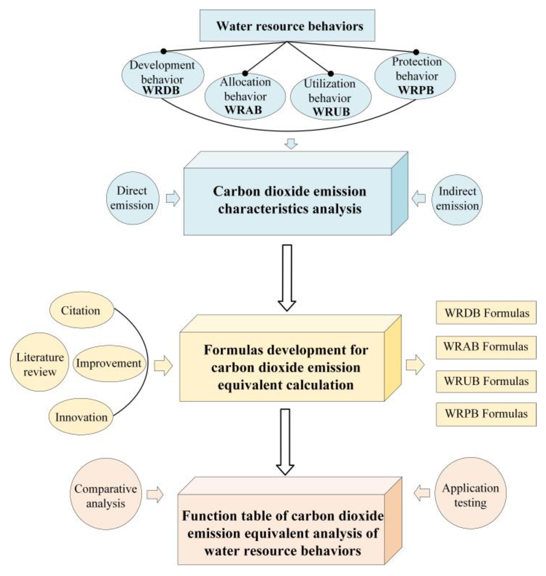
This study proposes the CEEA method and develops the FT-CEEA (the function table of carbon dioxide emission equivalent analysis), aiming to find a reference “ruler” to provide methodological reference and technical support for the accounting of CEE related to WRBs. The general idea of the CEEA method is to develop diversified CEE functions for WRBs in different dimensions by direct reference, refinement, and innovation, and finally integrate them into a unified calculation platform to form a relatively complete “ruler”, namely FT-CEEA. The general idea diagram of the CEEA method is shown in Figure 1.
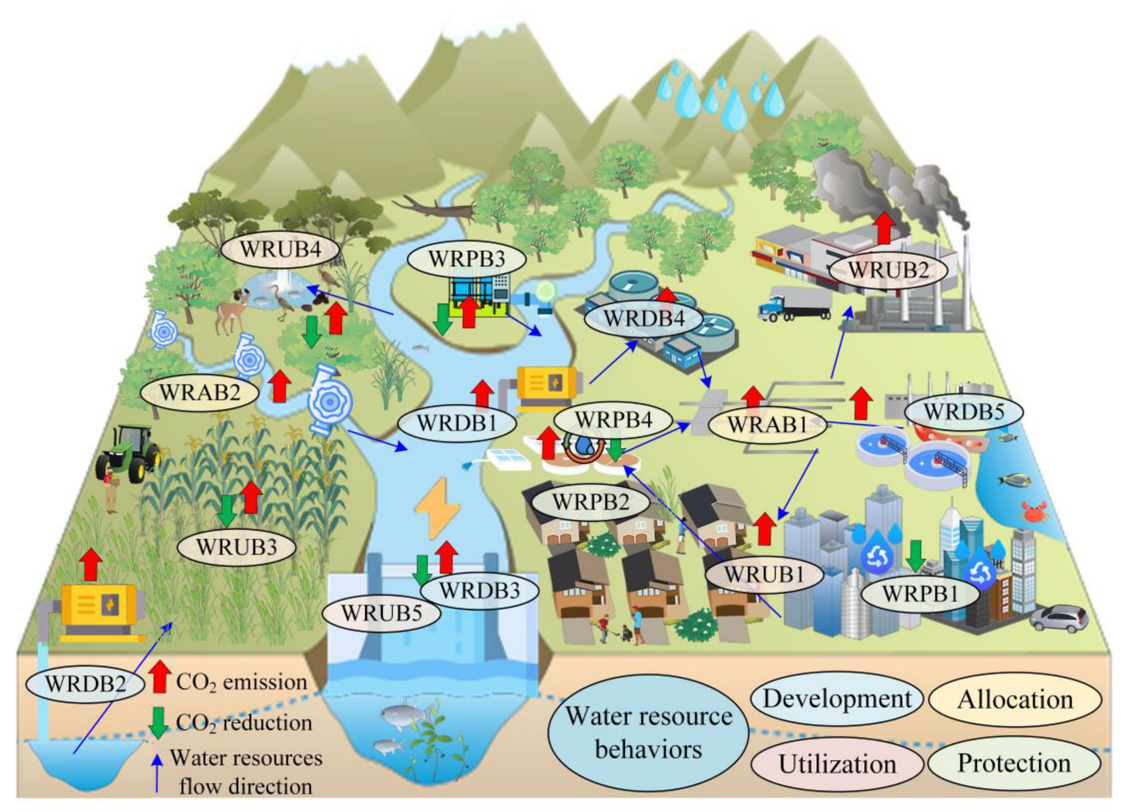
The WRBs involve a wide range of fields and factors, and the CEE accounting of WRBs should have a clear system boundary to avoid the infinite extension of indirect calculations. The principle of this study for system boundary formulation is to focus on CEE directly caused by WRBs, with appropriate consideration of indirect CEE that are closely related to such WRBs. Based on the definition of WRBs, the system boundary of CEE accounting is determined, as shown in Figure 2. The categories of WRBs can be roughly divided into water resource development behaviors (WRDBs), water resource allocation behaviors (WRABs), water resource utilization behaviors (WRUBs), and water resource protection behaviors (WRPBs). Each category contains a variety of typical WRBs, each WRB has a corresponding CEEA method.
2.2. CEEA Method to Water Resource Development Behaviors
Water resource development behaviors (WRDBs) refer to a series of activities related to water resources development. In this study, WRDBs are preliminarily defined as surface water lifting (WRDB1), groundwater extraction (WRDB2), reservoir storage (WRDB3), raw water treatment (WRDB4), and seawater desalination (WRDB5).
(1) Surface water lifting (WRDB1): Surface water resources are extracted from natural rivers or lakes to higher elevations using water extraction projects to achieve centralized treatment and unified distribution of “raw freshwater”. The electric energy consumed by the water lifting project is converted into the mechanical energy needed for water resources lifting, so the CO2 emissions of this behavior are mainly concentrated in the energy consumption link of the water lifting project. The CEEA formula of WRDB1 based on emission factor [52] is as follows:
where E1 is the carbon dioxide emission equivalent of surface water lifting behavior, kg; Q1 is the amount of surface water lifting, m3; EI1 is the energy intensity of WRDB1 (the amount of electricity required to lift per unit of surface water) kWh/m3; ρ is the density of surface water (typically 1000), kg/m3; g is the acceleration of gravity (typically 9.8), m/s2; h1 is the surface water lifting head, m; η is the efficiency of the water lifting project; EI1 is the power system CO2 emission factor (the amount of CO2 emitted per unit of electricity consumed), kg/kWh; EG is the total net power generation during the calculation period of the power system, kWh; FC is the consumption of fuel by the generator set during the calculation period, in mass or volume units; NCV is the average low-level heat content of the fuel during the calculation period, in GJ/mass or volume units; EFCO2 is the CO2 emission factor of the fuel (amount of CO2 emitted per unit of energy) during the calculation period, kgCO2/GJ; i is the type of fossil fuels consumed to generate electricity; and y is the year. Power-related departments in different countries will regularly release the EF of the power system. For example, the Ministry of Ecology and Environment of China has issued EF reference values for different provinces in China. In China, EI1 is mainly related to the water head, which can be 0.2 kWh/m3 [53,54] on average. The global level can refer to the value range given by relevant research: 0.0002–1.74 kWh/m3 [55].
(2) Groundwater extraction (WRDB2): Similar to the principle of WRDB1, groundwater extraction behavior also needs to convert the electrical energy of pumping equipment into the mechanical energy required for groundwater rise. CO2 emissions are mainly concentrated in the energy consumption of pumping equipment:
where E2 is the CEE of WRDB2, kg; Q2 is the amount of groundwater extraction, m3; EI2 is the energy intensity of WRDB2 (the amount of electricity required to extract per unit of groundwater) kWh/m3; h2 is the groundwater depth, m. Other variables have the same meaning as above. Unlike surface water, the energy intensity of WRDB2 varies considerably with different groundwater burial depths. The value of EI2 can be obtained according to the actual situation of the study area, and EI2 in different regions of China can also refer to Table 4 [39]. In addition, the EI2 of different countries is available in studies: 0.18–0.49 kWh/m3 (USA) [56], 0.48–0.53 kWh/m3 (Australia) [57], and 0.37–1.44 kWh/m3 (Global) [55].
(3) Reservoir storage (WRDB3): The energy consumption of WRDB3 mainly comes from the daily operation and management of water storage infrastructure [54], such as gate control, lighting, and monitoring equipment operation. This process also produces CO2 emissions. The calculation formula is as follows:
where E3 is the CEE of WRDB3, kg; Q3 is the actual volume of water stored in the reservoir, m3; EI3 is the energy intensity of WRDB3 (the amount of electricity required to store per unit of water in the reservoir) kWh/m3. EI3 varies due to differences in reservoir conditions in different regions. Field visits to reservoirs can be conducted to obtain the value of EI3. EI3 can also refer to existing research. Studies have shown that the energy intensity range of WRDB3 in China is [0.07,0.2] kWh/m3 [54], and 0.14 kWh/m3 can be used to study the average state of China [58].
(4) Raw water treatment (WRDB4): After taking raw water from the water source, it needs to be treated by the waterworks, including coagulation, sedimentation, filtration, and disinfection [41]. Each process relies mainly on electricity to maintain the normal operation of the processing equipment, so WRDB4 also produces CO2 emissions [51]:
where E4 is the CEE of WRDB4, kg; Q4 is the volume of raw water treatment, m3; EI4 is the energy intensity of WRDB4 (the amount of electricity required to treat per unit of raw water) kWh/m3. EI4 can be determined by the statistical calculation of energy consumption data of each link of WRDB4. According to the yearbook of Chinese urban water supply, the national average is 0.31 kWh/m3 [54,59], which can be used for reference. Existing studies have also given the values of different countries for reference: 0.371–0.392 kWh/m3 (USA) [56]; 0.1–0.6 kWh/m3 (Australia) [60]; 0.38–1.44 kWh/m3 (Canada) [61]; 0.11–1.5 kWh/m3 (Spain) [62]; 0.15–0.44 kWh/m3 (New Zealand) [63].
(5) Seawater Desalination (WRDB5): Nine coastal provinces in China have large-scale seawater desalination capacity. Although the industrialization process of desalination in China is slow, seawater desalination is an important behavior in the process of sustainable development of water resources in the future [51].
where E5 is the CEE of WRDB5, kg; Q5 is the volume of seawater desalination, m3; EI5 is the energy intensity of WRDB5 (the amount of electricity required to treat per unit of seawater) kWh/m3; EI5 should be obtained based on the survey data of desalination plants, and can also refer to existing studies: 5.9 kWh/m3 (China) [64,65,66]; 4 kWh/m3 (Australia) [57]; 2.4–8.5 kWh/m3 (Global) [55,67].
2.3. CEEA Method to Water Resource Allocation Behaviors
Water resource allocation behaviors (WRABs) refer to a series of activities related to water resource transportation and distribution. Representative WRABs include urban-rural tap water allocation (WRAB1) and inter-regional water transfer (WRAB2).
(1) Tap water allocation (WRAB1): The treated water from the waterworks is distributed to individual water users through the urban and rural water distribution system. The energy consumption of WRAB1 is mainly the head loss in the water transmission and distribution process, and the CEE is focused on the power consumption in the pressurization process [68]:
where E6 is the CEE of WRAB1, kg; Q6 is the amount of urban and rural tap water allocation, m3; EI6 is the energy intensity of WRAB1 (the amount of electricity required to distribute per unit of tap water) kWh/m3; hf is head loss along the path, λ is the drag coefficient along the path, l is the length of tap water allocation, R is the hydraulic radius, m; v is the average velocity of tap water transmission and distribution, m3/s; hj is local head loss, m; ζ is local drag coefficient; η is the efficiency of the pressurized pump station. Head loss can be calculated by the Darcy formula. EI6 can be obtained according to the investigation and statistics of unit water distribution power consumption data of water supply company. The energy intensity of tap water companies in different regions of China is quite different [69]. Combined with the China Urban Water Supply Yearbook and related research [68,69,70], the recommended value is 0.2 kWh/m3 for reference. Reference values of EI6 in other countries: 0.2–0.32 kWh/m3 (California, USA) [26]; 0.12–0.22 kWh/m3 (Spain) [71]; 0.1 kWh/m3 (South Africa) [72].
(2) Inter-regional water transfer (WRAB2): Most of the inter-regional water transfer projects require pumping stations for pressurized delivery to overcome the energy loss from head loss. The CEE calculation principle of WRAB2 is similar to that of WRAB1. The difference is that the urban and rural tap water allocation system is mostly pressure pipe flow, while the inter-regional water transfer is mostly open channel constant flow:
where E7 is the CEE of WRAB2, kg; Q7 is the amount of water transferred across regions, m3; EI7 is the energy intensity of WRAB2 (the amount of electricity required to transfer per unit water resources across regions) kWh/m3; hf and hj are the head loss along the open channel and local head loss, m; the specific calculation can be referred to the relevant formula of open channel hydraulics [73]. In the absence of the necessary investigation conditions, EI7 can refer to the value of 0.815 kWh/m3 (China) taken in existing studies [54,74].
2.4. CEEA Method to Water Resource Utilization Behaviors
Water resource utilization behaviors (WRUBs) refer to a series of activities related to water use. WRUBs include domestic water utilization (WRUB1), industrial water utilization (WRUB2), agricultural water utilization (WRUB3), ecological water utilization (WRUB4), and hydroelectric power generation (WRUB5). Many carbon emission studies based on LCA methods do not consider the end-use process, because the emission effects caused by end-use are not part of the life cycle [29]. However, some indirect emission effects closely related to WRBs are generated or caused by these behaviors, and end-use often results in a high proportion of CEE [27]. Therefore, based on the definition of WRBs, this study also includes CEE in the end-use process of water resources in the calculation range.
(1) Domestic water utilization (WRUB1): WRUB1 does not include public domestic water because the end-use purpose of public domestic water is so broad that it is difficult to achieve a relatively accurate quantification. The main source of CO2 emissions from WRUB1 is the energy consumption of the heating process [27]. Combined with the actual domestic water consumption in China, CO2 emissions in the energy-consuming process of cooking and bath heating can be taken as the CEE of WRUB1, and its CEEA method is as follows:
where E8 is the CEE of WRUB1, kg; Q8 is the total amount of domestic water consumption, m3; ρ is the density of surface water (typically 1000), kg/m3; Cw is the heat capacity of the water (generally 1.162 × 10⁻³ kWh/(kg·°C) [74]); ∆T is the temperature difference before and after heating, °C; η is the efficiency of the heating equipment (generally 95% [74]). Rhousehold is the proportion of residential household domestic water consumption in total domestic water consumption; Rheat is the proportion of water used for heating in residential household domestic water consumption, where Rheat1 is the proportion of cooking and drinking water, and Rheat2 is the proportion of bathing water. Depending on different research needs, Rhousehold can be obtained according to the actual investigation, or according to the proportion in the water resources bulletin. In addition, studies have examined the energy intensity (EI8) of household water use in different regions for reference: 7.43 kWh/m3 (China) [75], 24.6 kWh/m3 (Ontario, Canada) [61].
(2) Industrial water utilization (WRUB2): China has a wide range of industrial sectors, and the water use processes in different sectors have different CO2 emission characteristics. The energy consumption of WRUB2 is mainly concentrated in the link of water cooling and water heating [59], which is also the main source of CO2 emission. There are two ideas for calculating the CEE of WRUB2:
where E9 is the CEE of WRUB2, kg; Q9 is the total amount of industrial water consumption, m3; EI9 is the energy intensity of WRUB2 (energy consumption per unit of industrial water) kWh/m3. EI9 can be determined from field surveys, and relevant studies have concluded that the energy intensity of industrial water use in a typical Chinese city is 5.033 kWh/m3 [76]. Another idea is to calculate CEE by determining the power consumption of WRUB2 through the power consumption structure of the industrial sector [59]. A study suggests that water-related electricity consumption in the industrial sector in typical Chinese cities accounts for about 10% [59]. Cindustry is total industrial electricity consumption, kWh; Rwater is the ratio of water cooling and water heating power consumption to total power consumption in the industrial sector, %.
(3) Agricultural water utilization (WRUB3): Unlike domestic and industrial water, CO2 emissions from agricultural water utilization are mainly concentrated in the irrigation process. There are five main sources of carbon emissions from farmland ecosystems: chemical fertilizers, pesticides, agricultural films, agricultural machinery, and agricultural irrigation [77]. In this study, CO2 emissions from agricultural irrigation are used as the CEE of WRUB3. In addition, the carbon sink effect occurs on farmland due to photosynthesis during crop growth [78]. Therefore, the CO2 absorption effect of WRUB3 should be considered [79]. The three elements of crop growth are: sunlight, water, and fertilizer, and the carbon sink effect in farmland is the result of the joint action of these three elements. Obviously, it is not appropriate to consider the entire amount of CO2 absorbed by the farmland as the CO2 absorption effect of WRUB3. Therefore, the CO2 absorption effect of WRUB3 is separated from the overall CO2 absorption effect of farmland by setting weights. Assuming that the three elements of sunlight, water, and fertilizer are equally important for the crop growth process [80], the contribution of these three elements to the carbon sink effect can be distributed by equal weight method. Of course, the weight distribution scheme can be discussed and adjusted according to the actual situation of crop planting. The CEE calculation method of WRUB3 is as follows:
where E10 is the CEE of WRUB3, kg; E10emission is the total CO2 emissions of WRUB3, kg; E10absorption is the amount of CO2 absorbed by agricultural water utilization; A is the actual agricultural irrigation area, ha; δe and δa are CO2 emission and absorption coefficient per unit irrigated area, t/ha; ω is the weight, which is initially set to 1/3.
(4) Ecological water utilization (WRUB4): Water resources are the foundation and core of ecosystem functions. The function of ecosystems such as woodlands, grasslands, wetlands, and watersheds cannot be performed without the maintenance of ecological water [81]. WRUB4 refers to artificial ecological water, that is, urban environmental water and rivers, lakes, and wetland replenishment water supplied by human measures [82]. Different from domestic and production water utilization behaviors, the CEE of WRUB4 cannot be directly quantified by energy as a medium. Therefore, in this study, the CO2 absorbed by four land types closely related to ecological water use, namely, urban garden, urban green space (excluding garden area), water area within the jurisdiction, and wetland within the jurisdiction, is roughly taken as the CEE of WRUB4. Of course, the actual process of CO2 absorption from WRUB4 is far more complicated than described.
where E11 is the CEE of WRUB4, kg; A is the area of ecological water land type, ha; δ is the CO2 absorption coefficient of ecological water land type (the amount of CO2 absorbed per unit area of ecological water land), t/ha. i is the type of land. δ can be obtained by field measurements in the study area, or by referring to existing studies [78].
(5) Hydroelectric power generation (WRUB5): CO2 emissions from hydropower generation are much lower than those from thermal power [83]. Based on the UN CDM (United Nations’ Clean Development Mechanism), GHG emissions from hydropower generation can be disregarded in the calculation of hydropower CDM projects [84]. Therefore, the relative carbon reduction effect of hydropower compared to thermal power is used in this study to quantify the CEE of WRUB5.
where E12 is the CEE of WRUB5, kg; G is the total amount of hydroelectric power, kWh; CPG is the standard coal consumption of power generation unit, tce/kWh; EFc is the CO2 emission coefficient of standard coal, kg/tce. CPG can be obtained from the investigation of the thermal power industry in the study area. Studies have shown that the average coal consumption of thermal power generating units in China is 3.7 × 10⁻⁴ tce/kWh [85]. EFc can refer to IPCC guidelines for national greenhouse gas inventories [52] or existing studies [85].
2.5. CEEA Method to Water Resource Protection Behaviors
Water resource protection behaviors (WRPBs) refer to a series of activities related to water resources protection, including water saving (WRPB1), wastewater collection (WRPB2), wastewater treatment (WRPB3), and reclaimed water reuse (WRPB4).
(1) Water saving (WRPB1): Water saving behavior directly avoids part of the energy consumed in the development and allocation of water resources, so it can be regarded as a carbon reduction behavior [32,86]. Its CEEA method is as follows:
where E13 is the CEE of WRPB1, kg; Q13 is the total amount of water saved, m3; EPexploitation is the comprehensive CO2 emission coefficient of water resource exploitation (CO2 emissions per unit of water resource exploitation), kg/m3; EPdistribution is the comprehensive CO2 emission coefficient of water resource allocation (CO2 emissions per unit of water resource allocation), kg/m3. Other variables have the same meaning as above.
(2) Wastewater collection (WRPB2): Wastewater from different sources usually relies on gravity to converge to the wastewater network, and then is pressurized by the wastewater network pump to the wastewater treatment plant. Similar to WRAB1, the CEE of WRPB2 is mainly generated by energy consumption to overcome head loss [49]:
where E14 is the CEE of WRPB2, kg; Q14 is the total amount of wastewater collected, m3; EI14 is the energy intensity of WRPB2 (electricity consumption by collecting unit of wastewater), kWh/m3. EI14 should be obtained based on the investigation and statistics of the wastewater collection system in the study area, and can also refer to the values in related studies: 0.013 kWh/m3 (China) [86].
(3) Wastewater treatment (WRPB3): The treatment methods of wastewater treatment plants in different countries are different, but generally include three stages: primary treatment, secondary treatment, and tertiary treatment. Each stage has different processes, and the energy consumption intensity of each process is different. The main CO2 emissions are concentrated in the secondary and tertiary treatment stages [87]. On the other hand, untreated wastewater contains more pollutants such as COD and BOD5, which can produce large amounts of carbon emissions. WRPB3 has a positive CO2 reduction effect by reducing the concentration of such pollutants [88]. In addition, wastewater treatment plants generally use sludge in wastewater for power generation [89], and its carbon reduction effect should also be considered. In this study, the CO2 absorption effect of WRPB3 is considered based on the concentration difference of major carbon emission pollutants before and after wastewater treatment and the sludge power generation:
where E15 is the CEE of wastewater treatment behavior, kg; Q15 is the total amount of wastewater treatment, m3; EI15 is the energy intensity of WRPB3 (electricity consumption by treating unit of wastewater), kWh/m3. EIij is the energy consumption intensity of the process j in stage i, kWh/m3. The energy intensity or emission factor of unit wastewater treatment can be obtained by investigating the energy consumption and treatment capacity of the wastewater treatment plant [28,29]. EI15 from relevant studies are available for reference: 0.24 kWh/m3 (China) [74]; 0.8–1.5 kWh/m3 (Australia) [60]; 0.177–0.78 kWh/m3 (USA) [56]; 0.41–0.61 kWh/m3 (Spain) [71]; 0.44 kWh/m3 (South Africa) [72]; 0.38–1.122 kWh/m3 (Global) [55]. Rs is the sludge concentration in wastewater, generally 0.3–0.5% [90]; Ps is the power generation of unit sludge, and the coefficient in related research is 14.27 kWh/m3 for reference [89]. ∆RCOD and ∆RBOD5 are the concentration differences of COD and BOD5 before and after wastewater treatment, respectively. When the measurement conditions are available, the measurement results shall prevail. When conducting large-scale research, ∆RCOD and ∆RBOD5 can also be determined according to relevant emission standards. According to China’s comprehensive wastewater discharge standard, the concentration difference between COD and BOD5 before wastewater treatment (Level 3 standard) and after wastewater treatment (Level 1 standard) is 0.94 kg/m3 and 0.58 kg/m3. EFCOD and EFBOD5 are the amount of CO2 reduced by removing unit COD and BOD5, and the units are kgCO2/kgCOD and kgCO2/kgBOD5, respectively. According to the relevant emission factors released by IPCC [52], EFCOD and EFBOD5 are 0.69 and 1.65, respectively.
(4) Reclaimed water reuse (WRPB4): Reclaimed water reuse reduces the extraction of surface water and groundwater, and can therefore be considered as a WRB to reduce CO2 emissions. The calculation formula of CEE is as follows:
where E16 is the CEE of reclaimed water reuse behavior, kg; Q16 is the amount of reclaimed water reuse, m3; EP is the comprehensive CO2 emission coefficient of water resources exploitation (CO2 emissions per unit of water resource exploitation), kg/m3.
2.6. Function Table of CEEA for Water Resource Behaviors
The above methods and ideas are summarized and all the CEEA formulas are combined to form a table, which is the function table of CEEA (FT-CEEA) for WRBs (Table 2). In addition, in view of the large regional differences in the grid CO2 emission factor and the energy intensity of groundwater extraction, the referenceable values (Table 3 and Table 4) for different regions of China are given [54], which can be selected according to the actual situation of the study area. The instructions for using FT-CEEA are as follows.
(1) FT-CEEA is a collection of formulas for estimating and cross-sectionally comparing the CEE of various WRBs. The CEEA formulas for different WRBs in FT-CEEA can be used selectively depending on the study purpose and study scale. The quantity, type, and calculation method of WRBs in FT-CEEA are not static and can be updated and improved according to the changing situation and new research progress.
(2) The results of each formula are not necessarily an absolute measurement of the emission or absorption effects of CO2, but the idea of each formula is relatively reasonable. FT-CEEA is equivalent to setting up a “ruler” as a relative comparison of CEE generated by WRBs calculated by different researchers. FT-CEEA has no scale limitation and can be applied to different scales with limited accuracy requirements. However, the specific parameters need to be adjusted according to the actual situation of the research object.
(3) Most of the formulas in FT-CEEA need to be supported by relevant parameters, but in most cases, it is difficult to carry out field investigations and measurements of the parameters. Given this situation, some valuable reference values are provided in this table. Of course, some changes can be made in the selection of parameter reference values according to different research needs and actual conditions.
3. Case Study
3.1. Overview of the Study Area
China has a vast territory, and there are significant spatial differences in industrial structure, water use mode, and carbon emission intensity in different regions. In terms of CO2 emissions in 2019, Shanxi (the province with the highest emission intensity) is 37 times higher than Qinghai (the province with the lowest emission intensity) under different development orientation [91]. In the past 20 years, under the background of rapid economic and social development, some provinces in China are facing many challenges such as the insufficient capacity for sustainable utilization of water resources and prominent conflict between carbon emission reduction and economic development [92]. Since the 1990s, China has been in a new period of rapid growth in carbon emissions, lagging behind developed countries in time. Although China’s total carbon emissions ranked first in the world in recent years, China’s per capita carbon emissions are still far lower than developed countries. Many traditional industries in China still maintain a production mode with high consumption and high emission. Promoting the low-carbon transformation of traditional industries has become an urgent bottleneck to achieving China’s carbon neutrality goal [7].
3.2. Data source and Description
In addition to the important parameters in FT-CEEA, the data used in the case study are mainly the data of indicators involved in different WRBs of 31 provinces in China in 2020. The data involved in WRABs include tap water allocation and inter-regional water transfer. The data involved in WRUBs include domestic water consumption, industrial water consumption, actual agricultural irrigation area, land area of four kinds of artificial ecological water utilization, and hydroelectric power generation. The data involved in WRPBs include water saving, wastewater treatment, and reclaimed water reuse.
The sources of the above data include China Water Resources Bulletin 2020, China Seawater Utilization Bulletin 2020, Water Resources Bulletin of 31 provinces in 2020, China Statistical Yearbook 2021, China Water Statistical Yearbook 2021, China Energy Statistical Yearbook 2021, China Environmental Statistical Yearbook 2021, and China Urban Construction Statistical Yearbook 2021.
3.3. Results and Discussion
3.3.1. Carbon Dioxide Emission Equivalent Analysis of WRDBs
Based on FT-CEEA and the above data, the CEE of WRBs in 31 provinces and 8 regions of China in 2020 was calculated. The calculation results of the eight regions are obtained by summing the included provinces.
The CEEA results of WRDBs are presented in Table 5. In 2020, the surface water lifting behavior (WRDB1) in eight regions of China generated 63.52 million tons of CEE, accounting for 29.8% of the total CEE produced by WRDBs. Among them, the WRDB1 in middle Yangtze River and east coast provinces produced higher CEE of 12.63 million tons and 11.9 million tons, respectively. The three provinces of Shanghai, Jiangsu, and Zhejiang in the east coast region are dominated by surface water utilization. The surface water supply of Jiangsu Province in 2020 is 55.6 billion cubic meters, resulting in the CEE generated by WRDB1 ranking first among 31 provinces (8.18 million tons). The region with the smallest CEE of WRDB1 is the north coast region (4.64 million tons). On the other hand, WRDB2 in the north coast region produced the most CEE (8.2 million tons). In contrast, groundwater extraction in the east coast region produced only 0.12 million tons of CEE in 2020. The spatial distribution characteristics of CEEA results of WRDB1 and WRDB2 are closely related to the water supply structure in different regions. Compared with the southern provinces of China, the northern provinces have a higher degree of groundwater exploitation and a larger proportion of groundwater utilization, which is also a manifestation of the uneven spatial distribution of water resources in China [94]. In addition, Xinjiang is the province with the most CEE generated by WRDB2 in 31 provinces (5.69 million tons). The reason is that Xinjiang has a large amount of groundwater supply. In 2020, the groundwater supply in Xinjiang is 12.43 billion cubic meters, second only to Heilongjiang (12.94 billion cubic meters). Another important factor is that Xinjiang’s higher altitude means it takes much more energy to extract per unit of groundwater than the eastern provinces [39].
WRDB3 is the behavior that produces the most CEE in WRDBs, generating 75.9 million tons of CEE in 2020, accounting for 35.6% of the total CEE produced by WRDBs. Among them, the CEE produced in middle Yangtze River and southwest regions was significantly higher than that in other regions, and the CEE produced by WRDB3 in the east coast region was less (4.69 million tons). Raw water treatment behavior (WRDB4) produced 39.55 million tons of CEE in 2020. Due to the high proportion of domestic and industrial water, the east coast, the middle Yangtze River and the southern coastal provinces have become the main contributors to the CEE generated by WRDB4. In 2020, the CEE generated by seawater desalination behavior (WRDB5) was 2.92 million tons, accounting for 1.4% of the total CEE generated by WRDBs. China’s desalination plants are mainly concentrated in 9 coastal provinces [64], which are Shandong, Hebei, Zhejiang, Tianjin, Liaoning, Guangdong, Fujian, Hainan, and Jiangsu in descending order according to CEE. The proportion of CEE generated by WRDB5 in the north and east coast provinces exceeded 87%.
3.3.2. Carbon Dioxide Emission Equivalent Analysis of WRABs
The CEEA results of water resource allocation behaviors (WRABs) are shown in Table 5. WRAB1 produced 26.36 million tons of CEE in 2020, accounting for 60.9% of the total CEE produced by WRABs. The CEE of WRAB1 is similar to WRDB4 in spatial distribution. The difference in water resources utilization structure in different regions of China can explain the distribution characteristics to some extent. Compared with the eastern provinces of China, the northwest provinces have a higher proportion of agricultural water and a lower proportion of industrial and domestic water [95]. Tap water supply is mainly concentrated in industrial and domestic water. Therefore, the water use structure dominated by agricultural water has led to the CO2 emission effect of WRAB1 in the northwest region being much lower than that in the eastern region. Cross-regional water transfer behavior produced 16.95 million tons of CEE in 2020. Due to the existence of large-scale water diversion projects such as the South-to-North Water Diversion Project and the Luanhe River Diversion Project, the CEE generated by WRAB2 in the north coast and the middle Yellow River provinces accounted for up to 89%. This spatial distribution feature is similar to the research results of Xiang and Jia [54].
3.3.3. Carbon Dioxide Emission Equivalent Analysis of WRUBs
The CEEA results of WRUBs are shown in Table 6. Among the five kinds of WRUBs, the CEE value of domestic water utilization and industrial water utilization is positive, resulting in the CO2 emission effect. The CEE value of agricultural water utilization, ecological water utilization, and hydroelectric power generation is negative, resulting in the CO2 absorption effect. Among them, the CEE calculation of WRUB2 is based on the first calculation scheme (energy intensity scheme).
In 2020, the CEE of WRUB1 (326.88 million tons) and WRUB2 (353.54 million tons) in 31 provinces of China are not very different in total, but there are large differences between regions. The CEE generated by WRUB2 in the east coast and middle Yangtze River provinces is higher than that generated by WRUB1, especially in the east coast provinces. The outstanding proportion of industrial and domestic water in Jiangsu Province leads to the highest CEE generated by WRUB2. The difference in water use structure is the main reason for the difference in CEE of industrial and domestic water in different regions [96]. The absorption effect of WRUB3 (288.84 million tons) is greater than the emission effect (57.02 million tons), so the CEE of agricultural water utilization behavior is negative in total (−231.83 million tons). The WRUB3 of the northwest provinces has produced a considerable CO2 emission effect (6.48 million tons), which is consistent with the local water resource utilization structure [97]. The middle Yangtze River provinces have more agricultural irrigation area, and the CO2 absorption effect produced by WRUB3 is also the highest among the eight regions (51.9 million tons).
Ecological water utilization behavior (WRUB4) produced −144.06 million tons of CEE in 2020. The CEE of WRUB4 in southwest and northwest provinces was nearly half of the total CEE produced by WRUB4. The main reason is that the wetland and water area of Sichuan, Tibet, Qinghai, Xinjiang, and other provinces is much higher than other regions. The strong guarantee of ecological water use in the above-mentioned provinces has played an important role in maintaining the carbon sink function of wetland and water ecosystem [98]. In 2020, the hydroelectric power generation behavior (WRUB5) in eight regions of China produced a total of −335.95 million tons of CEE with significant spatial differences. Southwest provinces have the most abundant hydropower resources [99], while the proportion of hydropower in the energy structure of the north coast provinces is very small. The distribution of hydropower resources in China is the main reason for the CEE spatial difference of WRUB5.
3.3.4. Carbon Dioxide Emission Equivalent Analysis of WRPBs
The CEEA results of WRPBs are shown in Table 7. Among the four WRPBs, only the CEE value of wastewater collection behavior (WRPB2) is positive, resulting in CO2 emission effect. The CEE values of the other three WRPBs are negative, resulting in the CO2 absorption effect. Water saving behavior (WRPB1) can undoubtedly provide a positive impact on reducing CO2 emissions [100]. If only the energy saving effect of WRPB1 on water resources development and allocation is considered, the CEE of WRPB1 in 2020 is −2.05 million tons. In general, Shanghai, Guangdong, Zhejiang, Jiangsu, and Beijing are at the forefront of the construction of water-saving society [101], and there is still a large room for improvement in the capacity of water-saving and emission reduction in northwest provinces. The CEE of WRPB2 is the smallest among all WRBs in FT-CEEA (0.5 million tons). The CO2 absorption effect produced by wastewater treatment behavior (WRPB3) is significantly greater than the emission effect. The spatial distribution characteristics of CEE of WRPB3 are directly related to the wastewater treatment capacity of different regions. The east coast and south coast provinces have a large amount of wastewater discharge and a strong wastewater treatment capacity [102], which correspondingly brings a higher carbon dioxide emission and absorption effect. If only the energy saving effect of reclaimed water reuse behavior on water resources development is considered, the CEE generated by WRPB4 in 2020 is −2.68 million tons. The CEEA results of WRPB4 are closely related to regional water resource endowment and water supply structure. Compared with the southern provinces, Beijing, Hebei, Shandong, Henan, and other northern provinces are relatively short of water, so the reuse of reclaimed water has become an effective means to alleviate the contradiction between local water supply and demand [103]. As a result, the amount of reclaimed water supplied by these provinces is much higher than that of other provinces, and correspondingly, more CO2 absorption effect is generated.
4. Conclusions
In this study, the carbon dioxide emission equivalent analysis (CEEA) method of water resource behaviors (WRBs) was developed, and a function table of carbon dioxide emission equivalent (FT-CEEA) was constructed. Based on the FT-CEEA, the CEE of different WRBs in 31 provinces of China in 2020 was analyzed. Some valuable conclusions are as follows:
- (1)
- Four categories of WRBs in 31 provinces of China produced a total of 0.137 billion tons of CEE in 2020, of which the emission effect was 1.001 billion tons and the absorption effect was 0.864 billion tons. There is significant spatial variability in CEE of WRBs in eight regions of China, and the spatial distribution characteristics of CEE produced by different WRBs are also different. Water supply/utilization structure, energy consumption structure, water resources endowment, physical geographic characteristics, hydropower resources distribution are important reasons for the spatial differences of CEE.
- (2)
- The WRDBs and WRABs produced a total of 0.256 billion tons of CEE. Among the WRDBs, reservoir storage and surface water lifting have the most CO2 emission effect. Among the WRABs, the CEE from inter-regional water transfer is smaller than that from tap water allocation. Water resource protection behaviors produced −87 million tons of CEE. The absorption effect of wastewater treatment behavior is the main contributor to CEE, followed by reclaimed water reuse behavior and water saving behavior.
- (3)
- The CO2 emission and absorption effects of WRUBs are most significant among four categories. Domestic water and industrial water utilization are the two main sources of emission effects, hydroelectric power generation behavior produced the greatest absorption effect. There is still a certain distance to achieve carbon neutrality in the field of water resources.
Based on the above conclusions, some targeted measures and suggestions are discussed for the carbon neutrality goal in the field of water resources. Increasing the proportion of hydropower generation, improving the capacity of ecological water security, strengthening wastewater treatment and reclaimed water reuse, and promoting the construction of water-saving society can be considered as effective ways to promote carbon neutrality in this field.
However, there are still some limitations. The consideration of water resource behavior categories may not be comprehensive. In this study, the water resource behaviors were divided into four categories: development, allocation, utilization, and protection. However, water resource behaviors are not limited to the four categories, and the number of WRBs is far more than 16. Therefore, FT-CEEA is dynamic rather than static, and needs to be constantly updated. In addition, many CEE calculations of WRB are completed by using energy as an intermediate medium, which is the quantitative scheme adopted by most related studies. Although the energy consumption is the major factor in the generation of CEE by those WRBs, it cannot be excluded that there may be other potential factors contributing to carbon emissions. When these potential factors reach a certain scale, the resulting CEE also needs to be considered. Moreover, for some WRBs, the CEEA method may not be considered perfect. For example, the CO2 absorbed by the four types of land closely related to ecological water utilization was roughly used as the CEE of WRUB3. In fact, the CO2 absorbed by the lands is due to many factors, including ecological water utilization. How to separate the CEE of ecological water and CEE produced by other factors? Further exploration and refinement are still needed.
Author Contributions
Conceptualization, formal analysis, funding acquisition, project administration, Q.Z.; data curation, methodology, software, visualization, writing—original draft, Z.Z., C.Z. and X.Q.; investigation, J.M., Z.Z., C.Z., and X.Q.; supervision, Q.Z. and J.M.; resources, Q.Z. and Z.Z.; writing—review and editing, Q.Z., Z.Z., J.M., C.Z. and X.Q. All authors have read and agreed to the published version of the manuscript.
Funding
This research was funded by the Natural Science Foundation of China (no. 52279027), the National Key Research and Development Program of China (no. 2021YFC3200201), and the Major Science and Technology Projects for Public Welfare of Henan Province (no. 201300311500).
Institutional Review Board Statement
Not applicable.
Informed Consent Statement
Not applicable.
Data Availability Statement
Publicly available datasets were analyzed in this study. These data can be found and downloaded on relevant websites.
Conflicts of Interest
The authors declare no conflict of interest.
References
- Michalak, A.M. Study role of climate change in extreme threats to water quality. Nature 2016, 535, 349–350. [Google Scholar] [CrossRef] [PubMed] [Green Version]
- Hermwille, L.; Obergassel, W.; Ott, H.E.; Beuermann, C. UNFCCC before and after Paris–what’s necessary for an effective climate regime? Clim. Policy 2017, 17, 150–170. [Google Scholar] [CrossRef]
- Christoff, P. The promissory note: COP 21 and the Paris Climate Agreement. Environ. Politics 2016, 25, 765–787. [Google Scholar] [CrossRef]
- Azar, C.; Johansson, D.J.A. IPCC and the effectiveness of carbon sinks. Environ. Res. Lett. 2022, 17, 041004. [Google Scholar] [CrossRef]
- Salvia, M.; Reckien, D.; Pietrapertosa, F.; Eckersley, P.; Spyridaki, N.-A.; Krook-Riekkola, A.; Olazabal, M.; De Gregorio Hurtado, S.; Simoes, S.G.; Geneletti, D.; et al. Will climate mitigation ambitions lead to carbon neutrality? An analysis of the local-level plans of 327 cities in the EU. Renew. Sustain. Energy Rev. 2021, 135, 110253. [Google Scholar] [CrossRef]
- Mallapaty, S. How China could be carbon neutral by mid-century. Nature 2020, 586, 482–483. [Google Scholar] [CrossRef]
- Liu, Z.; Deng, Z.; He, G.; Wang, H.; Zhang, X.; Lin, J.; Qi, Y.; Liang, X. Challenges and opportunities for carbon neutrality in China. Nat. Rev. Earth Environ. 2022, 3, 141–155. [Google Scholar] [CrossRef]
- Wu, Y.; Xu, B. When will China’s carbon emissions peak? Evidence from judgment criteria and emissions reduction paths. Energy Rep. 2022, 8, 8722–8735. [Google Scholar] [CrossRef]
- Mancini, M.S.; Galli, A.; Niccolucci, V.; Lin, D.; Bastianoni, S.; Wackernagel, M.; Marchettini, N. Ecological Footprint: Refining the carbon Footprint calculation. Ecol. Indic. 2016, 61, 390–403. [Google Scholar] [CrossRef]
- Wiedmann, T.; Minx, J.; Barrett, J.; Wackernagel, M. Allocating ecological footprints to final consumption categories with input–output analysis. Ecol. Econ. 2006, 56, 28–48. [Google Scholar] [CrossRef]
- Dong, H.; Geng, Y.; Xi, F.; Fujita, T. Carbon footprint evaluation at industrial park level: A hybrid life cycle assessment approach. Energy Policy 2013, 57, 298–307. [Google Scholar] [CrossRef]
- Lenzen, M.; Sun, Y.-Y.; Faturay, F.; Ting, Y.-P.; Geschke, A.; Malik, A. The carbon footprint of global tourism. Nat. Clim. Chang. 2018, 8, 522–528. [Google Scholar] [CrossRef]
- Lombardi, M.; Laiola, E.; Tricase, C.; Rana, R. Assessing the urban carbon footprint: An overview. Environ. Impact Assess. Rev. 2017, 66, 43–52. [Google Scholar] [CrossRef]
- Onat, N.C.; Kucukvar, M. Carbon footprint of construction industry: A global review and supply chain analysis. Renew. Sustain. Energy Rev. 2020, 124, 109783. [Google Scholar] [CrossRef]
- Radonjič, G.; Tompa, S. Carbon footprint calculation in telecommunications companies—The importance and relevance of scope 3 greenhouse gases emissions. Renew. Sustain. Energy Rev. 2018, 98, 361–375. [Google Scholar] [CrossRef]
- Henriksson, P.J.G.; Heijungs, R.; Dao, H.M.; Phan, L.T.; De Snoo, G.R.; Guinée, J. Product Carbon Footprints and Their Uncertainties in Comparative Decision Contexts. PLoS ONE 2015, 10, e0121221. [Google Scholar] [CrossRef]
- Chai, C.; Zhang, D.; Yu, Y.; Feng, Y.; Wong, M.S. Carbon Footprint Analyses of Mainstream Wastewater Treatment Technologies under Different Sludge Treatment Scenarios in China. Water 2015, 7, 918–938. [Google Scholar] [CrossRef]
- Zhou, Y.; Chen, M.; Tang, Z.; Mei, Z. Urbanization, land use change, and carbon emissions: Quantitative assessments for city-level carbon emissions in Beijing-Tianjin-Hebei region. Sustain. Cities Soc. 2021, 66, 102701. [Google Scholar] [CrossRef]
- Raymond, P.A.; Hartmann, J.; Lauerwald, R.; Sobek, S.; McDonald, C.; Hoover, M.; Butman, D.; Striegl, R.; Mayorga, E.; Humborg, C.; et al. Global carbon dioxide emissions from inland waters. Nature 2013, 503, 355–359. [Google Scholar] [CrossRef] [Green Version]
- Keller, P.S.; Marcé, R.; Obrador, B.; Koschorreck, M. Global carbon budget of reservoirs is overturned by the quantification of drawdown areas. Nat. Geosci. 2021, 14, 402–408. [Google Scholar] [CrossRef]
- Guotong, Q.; Fei, C.; Na, W.; Dandan, Z. Inter-annual variation patterns in the carbon footprint of farmland ecosystems in Guangdong Province, China. Sci. Rep. 2022, 12, 14134. [Google Scholar] [CrossRef] [PubMed]
- Ran, Y.; Li, X.; Sun, R.; Kljun, N.; Zhang, L.; Wang, X.; Zhu, G. Spatial representativeness and uncertainty of eddy covariance carbon flux measurements for upscaling net ecosystem productivity to the grid scale. Agric. For. Meteorol. 2016, 230–231, 114–127. [Google Scholar] [CrossRef] [Green Version]
- Feng, X.; Fu, B.; Lu, N.; Zeng, Y.; Wu, B. How ecological restoration alters ecosystem services: An analysis of carbon sequestration in China’s Loess Plateau. Sci. Rep. 2013, 3, 2846. [Google Scholar] [CrossRef] [PubMed] [Green Version]
- Thompson, R.L.; Lassaletta, L.; Patra, P.K.; Wilson, C.; Wells, K.C.; Gressent, A.; Koffi, E.N.; Chipperfield, M.P.; Winiwarter, W.; Davidson, E.A.; et al. Acceleration of global N2O emissions seen from two decades of atmospheric inversion. Nat. Clim. Chang. 2019, 9, 993–998. [Google Scholar] [CrossRef]
- Fernández-Martínez, M.; Sardans, J.; Chevallier, F.; Ciais, P.; Obersteiner, M.; Vicca, S.; Canadell, J.G.; Bastos, A.; Friedlingstein, P.; Sitch, S.; et al. Global trends in carbon sinks and their relationships with CO2 and temperature. Nat. Clim. Chang. 2018, 9, 73–79. [Google Scholar] [CrossRef] [Green Version]
- Trask, M. Water-Energy Relationship; California Energy Commission: Sacramento, CA, USA, 2005. [Google Scholar]
- Griffiths-Sattenspiel, B.; Wilson, W. The Carbon Footprint of Water; River Network: Portland, OR, USA, 2009. [Google Scholar]
- Wakeel, M.; Chen, B.; Hayat, T.; Alsaedi, A.; Ahmad, B. Energy consumption for water use cycles in different countries: A review. Appl. Energy 2016, 178, 868–885. [Google Scholar] [CrossRef]
- Rothausen SG, S.A.; Conway, D. Greenhouse-gas emissions from energy use in the water sector. Nat. Clim. Change 2011, 1, 210–219. [Google Scholar] [CrossRef]
- Friedrich, E.; Pillay, S.; Buckley, C. Carbon footprint analysis for increasing water supply and sanitation in South Africa: A case study. J. Clean. Prod. 2009, 17, 1–12. [Google Scholar] [CrossRef]
- Li, R.; Zhao, R.; Xie, Z.; Xiao, L.; Chuai, X.; Feng, M.; Zhang, H.; Luo, H. Water–energy–carbon nexus at campus scale: Case of North China University of Water Resources and Electric Power. Energy Policy 2022, 166, 113001. [Google Scholar] [CrossRef]
- Valek, A.M.; Sušnik, J.; Grafakos, S. Quantification of the urban water-energy nexus in México City, México, with an assessment of water-system related carbon emissions. Sci. Total Environ. 2017, 590, 258–268. [Google Scholar] [CrossRef]
- Sambito, M.; Freni, G. LCA Methodology for the Quantification of the Carbon Footprint of the Integrated Urban Water System. Water 2017, 9, 395. [Google Scholar] [CrossRef] [Green Version]
- Fang, A.; Newell, J.P.; Cousins, J. The energy and emissions footprint of water supply for Southern California. Environ. Res. Lett. 2015, 10, 114002. [Google Scholar] [CrossRef]
- Boulos, P.F.; Bros, C.M. Assessing the carbon footprint of water supply and distribution systems. J. Am. Water Work. Assoc. 2010, 102, 47–54. [Google Scholar] [CrossRef]
- Heihsel, M.; Lenzen, M.; Malik, A.; Geschke, A. The carbon footprint of desalination: An input-output analysis of seawater re-verse osmosis desalination in Australia for 2005–2015. Desalination 2019, 454, 71–81. [Google Scholar] [CrossRef]
- Siddiqi, A.; Fletcher, S. Energy intensity of water end-uses. Curr. Sustain./Renew. Energy Rep. 2015, 2, 25–31. [Google Scholar] [CrossRef]
- Escriva-Bou, A.; Lund, J.R.; Pulido-Velazquez, M. Modeling residential water and related energy, carbon footprint and costs in California. Environ. Sci. Policy 2015, 50, 270–281. [Google Scholar] [CrossRef] [Green Version]
- Wang, J.; Rothausen, S.G.; Conway, D.; Zhang, L.; Xiong, W.; Holman, I.P.; Li, Y. China’s water–energy nexus: Greenhouse-gas emissions from ground-water use for agriculture. Environ. Res. Lett. 2012, 7, 014035. [Google Scholar] [CrossRef]
- Zeng, S.; Chen, X.; Dong, X.; Liu, Y. Efficiency assessment of urban wastewater treatment plants in China: Considering greenhouse gas emissions. Resour. Conserv. Recycl. 2017, 120, 157–165. [Google Scholar] [CrossRef]
- Zib, I.I.I.L.; Byrne, D.M.; Marston, L.T. Operational carbon footprint of the US water and wastewater sector’s en-ergy consumption. J. Clean. Prod. 2021, 321, 128815. [Google Scholar] [CrossRef]
- Marinelli, E.; Radini, S.; Foglia, A.; Lancioni, N.; Piasentin, A.; Eusebi, A.L.; Fatone, F. Validation of an evidence-based methodology to support regional carbon foot-print assessment and decarbonisation of wastewater treatment service in Italy. Water Res. 2021, 207, 117831. [Google Scholar] [CrossRef]
- Wu, Z.; Duan, H.; Li, K.; Ye, L. A comprehensive carbon footprint analysis of different wastewater treatment plant configurations. Environ. Res. 2022, 214, 113818. [Google Scholar] [CrossRef]
- Zhou, Y.; Zhang, B.; Wang, H.; Bi, J. Drops of Energy: Conserving Urban Water to Reduce Greenhouse Gas Emissions. Environ. Sci. Technol. 2013, 47, 10753–10761. [Google Scholar] [CrossRef] [PubMed]
- Parece, T.E.; Grossman, L.; Geller, E.S. Reducing Carbon Footprint of Water Consumption: A Case Study of Water Conservation at a University Campus. In The Handbook of Environmental Chemistry; Younos, T., Grady, C., Eds.; Springer: Berlin/Heidelberg, Germany, 2013; pp. 199–218. [Google Scholar] [CrossRef]
- Wang, J.; Chen, X.; Liu, Z.; Frans, V.F.; Xu, Z.; Qiu, X.; Xu, F.; Li, Y. Assessing the water and carbon footprint of hydropower stations at a national scale. Sci. Total. Environ. 2019, 676, 595–612. [Google Scholar] [CrossRef] [PubMed]
- Zhang, L.; Chen, S. Carbon peaks of water systems in Chinese cities under varying water demand dynamics and energy transition pathways. J. Clean. Prod. 2022, 379, 134695. [Google Scholar] [CrossRef]
- Venkatesh, G.; Chan, A.; Brattebø, H. Understanding the water-energy-carbon nexus in urban water utilities: Comparison of four city case studies and the relevant influencing factors. Energy 2014, 75, 153–166. [Google Scholar] [CrossRef]
- Bakhshi, A.A.; Demonsabert, S.M. Estimating the carbon footprint of the municipal water cycle. J. Am. Water Work. Assoc. 2012, 104, E337–E347. [Google Scholar] [CrossRef]
- Stokes, J.R.; Horvath, A. Energy and Air Emission Effects of Water Supply. Environ. Sci. Technol. 2009, 43, 2680–2687. [Google Scholar] [CrossRef] [Green Version]
- Presura, E.; Robescu, L.D. Energy use and carbon footprint for potable water and wastewater treatment. Proceedings of the International Conference on Business Excellence. 2017, Volume 11, pp. 191–198. Available online: https://sciendo.com/article/10.1515/picbe-2017-0020 (accessed on 17 January 2023).
- Eggleston, H.S.; Buendia, L.; Miwa, K.; Ngara, T.; Tanabe, K. 2006 IPCC Guidelines for National Greenhouse Gas Inventories; Institute for Global Environmental Strategies: Hayama, Japan, 2006. [Google Scholar]
- Hu, G.; Ou, X.; Zhang, Q.; Karplus, V.J. Analysis on energy–water nexus by Sankey diagram: The case of Beijing. Desalination Water Treat. 2013, 51, 4183–4193. [Google Scholar] [CrossRef]
- Xiang, X.; Jia, S. China’s water-energy nexus: Assessment of water-related energy use. Resour. Conserv. Recycl. 2019, 144, 32–38. [Google Scholar] [CrossRef]
- Plappally, A.K.; Lienhard, V.J.H. Energy requirements for water production, treatment, end use, reclamation, and disposal. Renew. Sustain. Energy Rev. 2012, 16, 4818–4848. [Google Scholar] [CrossRef]
- Appelbaum, B. Water and sustainability: US electricity consumption for water supply and treatment—The next half century. Water Supply. 2002, 4, 93. [Google Scholar]
- Rocheta, E.; Peirson, W. Urban Water Supply in a Carbon Constrained Australia; UNSW Water Research Centre: Kensington, Australia, 2011. [Google Scholar]
- Li, X.; Liu, J.; Zheng, C.; Han, G.; Hoff, H. Energy for water utilization in China and policy implications for integrated planning. Int. J. Water Resour. Dev. 2016, 32, 477–494. [Google Scholar] [CrossRef]
- He, G.; Zhao, Y.; Wang, J.; Zhu, Y.; Jiang, S.; Li, H.; Wang, Q. The effects of urban water cycle on energy consumption in Beijing, China. J. Geogr. Sci. 2019, 29, 959–970. [Google Scholar] [CrossRef] [Green Version]
- Marsh, D. The Water–Energy Nexus: A Comprehensive Analysis in the Context of New South Wales. Ph.D. Dissertation, Faculty of Engineering and Information Technology, University of Technology, Sydney, Australia, 2008. [Google Scholar]
- Maas, C. Ontario’s Water-Energy Nexus: Will We Find Ourselves in Hot Water or Tap into Opportunity? POLIS Project on Ecological Governance; University of Victoria: Victoria, BC, Canada, 2010. [Google Scholar]
- Muñoz, I.; Milà-i-Canals, L.; Fernández-Alba, A.R. Life cycle assessment of water supply plans in Mediterranean Spain: The Ebro river transfer versus the AGUA Programme. J. Ind. Ecol. 2010, 14, 902–918. [Google Scholar] [CrossRef]
- Kneppers, B.; Birchfield, D.; Lawton, M. Energy-water relationships in reticulated water infrastructure systems. Water Supply 2009, 76, 1–27. [Google Scholar]
- Lin, S.; Zhao, H.; Zhu, L.; He, T.; Chen, S.; Gao, C.; Zhang, L. Seawater desalination technology and engineering in China: A review. Desalination 2020, 498, 114728. [Google Scholar] [CrossRef]
- Liu, S.; Wang, Z.; Han, M.; Wang, G.; Hayat, T.; Chen, G. Energy-water nexus in seawater desalination project: A typical water production system in China. J. Clean. Prod. 2020, 279, 123412. [Google Scholar] [CrossRef]
- Buonomenna, M.G. Membrane processes for a sustainable industrial growth. RSC Adv. 2012, 3, 5694–5740. [Google Scholar] [CrossRef]
- von Medeazza, G.M. “Direct” and socially-induced environmental impacts of desalination. Desalination 2005, 185, 57–70. [Google Scholar] [CrossRef]
- Sharif, M.N.; Haider, H.; Farahat, A.; Hewage, K.; Sadiq, R. Water–energy nexus for water distribution systems: A literature review. Environ. Rev. 2019, 27, 519–544. [Google Scholar] [CrossRef]
- Smith, K.; Liu, S.; Liu, Y.; Guo, S. Can China reduce energy for water? A review of energy for urban water supply and wastewater treatment and suggestions for change. Renew. Sustain. Energy Rev. 2018, 91, 41–58. [Google Scholar] [CrossRef]
- He, G.; Zhao, Y.; Wang, J.; Li, H.; Zhu, Y.; Jiang, S. The water–energy nexus: Energy use for water supply in China. Int. J. Water Resour. Dev. 2018, 35, 587–604. [Google Scholar] [CrossRef]
- Corominas, J. Agua y energía en el riego, en la época de la sostenibilidad. Ing. Del Agua 2010, 17, 219–233. [Google Scholar] [CrossRef] [Green Version]
- Buckley, C.; Friedrich, E.; von Blottnitz, H. Life-cycle assessments in the South African water sector: A review and future challenges. Water SA 2011, 37, 719–726. [Google Scholar] [CrossRef] [Green Version]
- Sturm, T.W. Open Channel Hydraulics; McGraw-Hill: New York, NY, USA, 2001. [Google Scholar]
- Sousa, V.; Meireles, I. Dynamic simulation of the energy consumption and carbon emissions for domestic hot water production in a touristic region. J. Clean. Prod. 2022, 355, 131828. [Google Scholar] [CrossRef]
- Qiu, G.Y.; Zou, Z.; Li, W.; Li, L.; Yan, C. A quantitative study on the water-related energy use in the urban water system of Shenzhen. Sustain. Cities Soc. 2022, 80, 103786. [Google Scholar] [CrossRef]
- Zhao, R.; Yu, J.; Xiao, L.; Sun, J.; Luo, H.; Yang, W.; Chuai, X.; Jiao, S. Carbon emissions of urban water system based on water-energy-carbon nexus. Acta Geogr. Sin. 2021, 76, 3119–3134. [Google Scholar]
- Duan, H.P.; Zhang, Y.; Zhao, J.B.; Bian, X.M. Carbon footprint analysis of farmland ecosystem in China. J. Soil Water Conserv. 2011, 25, 203–208. [Google Scholar]
- Feng, M.; Zhao, R.; Huang, H.; Xiao, L.; Xie, Z.; Zhang, L.; Sun, J.; Chuai, X. Water–energy–carbon nexus of different land use types: The case of Zhengzhou, China. Ecol. Indic. 2022, 141, 109073. [Google Scholar] [CrossRef]
- Wu, H.; Guo, S.; Guo, P.; Shan, B.; Zhang, Y. Agricultural water and land resources allocation considering carbon sink/source and water scarcity/degradation footprint. Sci. Total. Environ. 2021, 819, 152058. [Google Scholar] [CrossRef]
- van Diepen, C.A.; Wolf, J.; van Keulen, H.; Rappoldt, C. WOFOST: A simulation model of crop production. Soil Use Manag. 1989, 5, 16–24. [Google Scholar] [CrossRef]
- Qiu, M.; Zuo, Q.; Wu, Q.; Yang, Z.; Zhang, J. Water ecological security assessment and spatial autocorrelation analysis of prefectural regions involved in the Yellow River Basin. Sci. Rep. 2022, 12, 5105. [Google Scholar] [CrossRef] [PubMed]
- Zuo, Q.; Zhou, K.; Yang, L. Study on the quantity of water resources and the water quantity for ecosystem use in water resources programming. Arid. Land Geogr. 2002, 4, 296–301. [Google Scholar]
- Xu, J.; Wang, F.; Lv, C.; Xie, H. Carbon emission reduction and reliable power supply equilibrium based daily scheduling towards hydro-thermal-wind generation system: A perspective from China. Energy Convers. Manag. 2018, 164, 1–14. [Google Scholar] [CrossRef]
- Whittington, R. Hydro and the CDM: The role of hydroelectricity in meeting Kyoto obligations. Refocus 2007, 8, 54–56. [Google Scholar] [CrossRef]
- Wu, B.; Chen, Y.; Zeng, Y.; Zhao, Y.; Yuan, C. Evaluation of carbon emission reduction in power generation and shipping of the Three Gorges Reservoir. Resour. Environ. Yangtze Basin 2011, 20, 257–261. [Google Scholar]
- Meng, F.; Liu, G.; Liang, S.; Su, M.; Yang, Z. Critical review of the energy-water-carbon nexus in cities. Energy 2019, 171, 1017–1032. [Google Scholar] [CrossRef]
- Racoviceanu, A.I.; Karney, B.W.; Kennedy, C.A.; Colombo, A.F. Life-Cycle Energy Use and Greenhouse Gas Emissions Inventory for Water Treatment Systems. J. Infrastruct. Syst. 2007, 13, 261–270. [Google Scholar] [CrossRef] [Green Version]
- Qamar, M.A.; Javed, M.; Shahid, S.; Iqbal, S.; Abubshait, S.A.; Abubshait, H.A.; Ramay, S.M.; Mahmood, A.; Ghaithan, H.M. Designing of highly active g-C3N4/Co@ ZnO ternary nanocomposites for the disinfection of pathogens and degradation of the organic pollutants from wastewater under visible light. J. Environ. Chem. Eng. 2021, 9, 105534. [Google Scholar] [CrossRef]
- Zhang, Q.; Sun, D.; Wang, M.; Yin, C. Analysis of Typical Energy Saving Technology in the Sewage Treatment Plant. Energy Procedia 2017, 142, 1230–1237. [Google Scholar] [CrossRef]
- Peng, L.; Nairuo, Z.; Wei, X. COD and Carbon Emission Reduction in Sludge Deep Dewatering Treatment and Disposal. Environ. Sanit. Eng. 2012, 20, 9–12. [Google Scholar]
- Guan, Y.; Shan, Y.; Huang, Q.; Chen, H.; Wang, D.; Hubacek, K. Assessment to China’s recent emission pattern shifts. Earth’s Future 2021, 9, e2021EF002241. [Google Scholar] [CrossRef]
- Wu, Q.; Zuo, Q.; Ma, J.; Zhang, Z.; Jiang, L. Evolution analysis of water consumption and economic growth based on Decomposition-Decoupling Two-stage Method: A case study of Xinjiang Uygur Autonomous Region, China. Sustain. Cities Soc. 2021, 75, 103337. [Google Scholar] [CrossRef]
- Li, D.; Zuo, Q.; Zhang, Z. A new assessment method of sustainable water resources utilization considering fair-ness-efficiency-security: A case study of 31 provinces and cities in China. Sustain. Cities Soc. 2022, 81, 103839. [Google Scholar] [CrossRef]
- Wang, Y.; Wang, Y.; Su, X.; Qi, L.; Liu, M. Evaluation of the comprehensive carrying capacity of interprovincial water resources in China and the spatial effect. J. Hydrol. 2019, 575, 794–809. [Google Scholar] [CrossRef]
- Liu, X.; Xu, Y.; Sun, S.; Zhao, X.; Wang, Y. Analysis of the Coupling Characteristics of Water Resources and Food Security: The Case of Northwest China. Agriculture 2022, 12, 1114. [Google Scholar] [CrossRef]
- Zhou, Y.; Ma, M.; Gao, P.; Xu, Q.; Bi, J.; Naren, T. Managing water resources from the energy-water nexus perspective under a changing climate: A case study of Jiangsu province, China. Energy Policy 2018, 126, 380–390. [Google Scholar] [CrossRef]
- Shi, Q.; Chen, S.; Shi, C.; Wang, Z.; Deng, X. The Impact of Industrial Transformation on Water Use Efficiency in Northwest Region of China. Sustainability 2014, 7, 56–74. [Google Scholar] [CrossRef] [Green Version]
- Yang, Q.; Liu, G.; Casazza, M.; Hao, Y.; Giannetti, B.F. Emergy-based accounting method for aquatic ecosystem services valuation: A case of China. J. Clean. Prod. 2019, 230, 55–68. [Google Scholar] [CrossRef]
- Li, X.-Z.; Chen, Z.-J.; Fan, X.-C.; Cheng, Z.-J. Hydropower development situation and prospects in China. Renew. Sustain. Energy Rev. 2018, 82, 232–239. [Google Scholar] [CrossRef]
- Shimizu, Y.; Toyosada, K.; Yoshitaka, M.; Sakaue, K. Creation of Carbon Credits by Water Saving. Water 2012, 4, 533–544. [Google Scholar] [CrossRef]
- Xu, Y.; Tian, Q.; Yu, Y.; Li, M.; Li, C. Water-Saving Efficiency and Inequality of Virtual Water Trade in China. Water 2021, 13, 2994. [Google Scholar] [CrossRef]
- Chen, K.; Liu, X.; Ding, L.; Huang, G.; Li, Z. Spatial Characteristics and Driving Factors of Provincial Wastewater Discharge in China. Int. J. Environ. Res. Public Health 2016, 13, 1221. [Google Scholar] [CrossRef]
- Yi, L.; Jiao, W.; Chen, X.; Chen, W. An overview of reclaimed water reuse in China. J. Environ. Sci. 2011, 23, 1585–1593. [Google Scholar] [CrossRef] [PubMed]
Figure 1.
The general idea of the CEEA method.

Figure 2.
Schematic diagram of CEE accounting for WRBs.

Figure 3.
The study area.


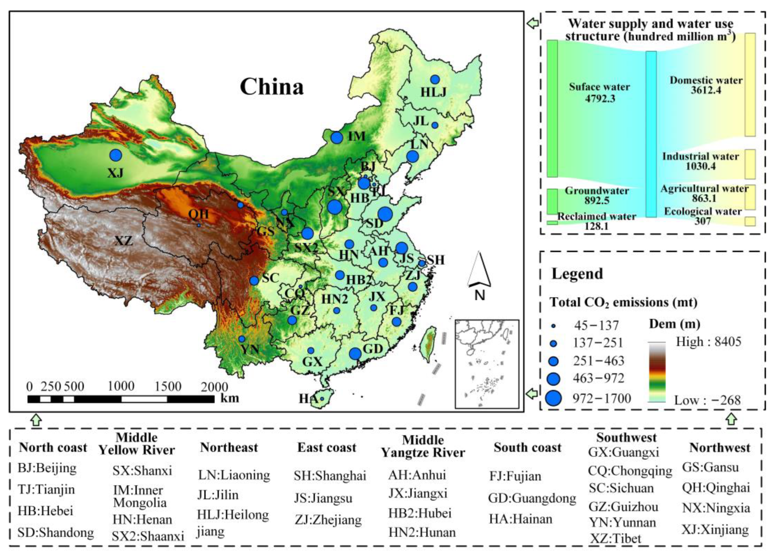
Table 1.
Selected representative literature of carbon emission effect studies in the field of water resources.
Table 1.
Selected representative literature of carbon emission effect studies in the field of water resources.
| Author(s) | Region(s) | Water-Related Activities | Methodology |
|---|---|---|---|
| Griffiths-Sattenspiel et al. [27] | United States | Water Supply and Conveyance | Carbon emission estimation based on statistical survey data and emission factors |
| Water Treatment | |||
| Water Distribution | |||
| Water End-Uses | |||
| Wastewater Collection and Treatment | |||
| Wastewater Discharge | |||
| Friedrich et al. [30] | Durban, South Africa | Water Impoundment | Carbon footprint analysis based on LCA method |
| Water Treatment | |||
| Water Distribution | |||
| Water Collection | |||
| Wastewater Treatment | |||
| Water Recycling | |||
| Bottled Water | |||
| Zhang et al. [47] | All cities in Guangdong Province, China | Water Extraction and Conveyance | Accounting for CO2 emissions based on energy intensity and emission factors |
| Water Purification and Supply | |||
| Water Distribution | |||
| Wastewater Treatment | |||
| Venkatesh et al. [48] | Nantes (France), Oslo (Norway), Turin (Italy), Toronto (Canada) | Water Supply | System analysis method |
| Water Treatment | |||
| Water Distribution | |||
| Wastewater Collection | |||
| Wastewater Treatment | |||
| Bakhshi and Demonsabert [49] | Loudoun, United States | Raw Water Extraction and Treatment | Carbon emission estimation based on survey data and Geographic information system models |
| Water Distribution | |||
| Wastewater Collection | |||
| Wastewater Treatment | |||
| Stokes and Horvath [50] | Southern California, United States | Imported Water | Carbon emission measurement of water supply system based on hybrid LCA method |
| Desalinated Ocean Water (Conventional pretreatment) | |||
| Desalinated Ocean Water (Membrane pretreatment) | |||
| Desalinated Brackish Groundwater | |||
| Recycled Water | |||
| Valek et al. [32] | México City, México | Water Supply | CO2 equivalent analysis based on statistical survey data and emission factors |
| Water Treatment System | |||
| Sambito and Freni [33] | Sicily, Italy | Water Supply and Treatment System | Carbon footprint analysis based on LCA approach |
| Distribution of Water and Sewer System | |||
| Wastewater Treatment Plant | |||
| Presura and Robescu [51] | Constanta, Romania | Potable Water Treatment | Carbon footprint analysis based on energy intensity and emission factors |
| Wastewater Treatment | |||
| Heihsel and Lenzen [36] | Australia | Seawater Desalination | Carbon footprint analysis based on multi-regional input-output model |
| Wang et al. [39] | China | Groundwater Use for Agriculture | Carbon footprint analysis based on energy intensity and emission factors |
| Wu et al. [43] | Australia | Wastewater Treatment (Direct emission) | Carbon footprint analysis based on emission factors |
| Wastewater Treatment (Indirect emission) | |||
| Wastewater Treatment (Value chain emission) |
Table 2.
FT-CEEA for water resource behaviors.
| WRBs | CEEA Formulas | Parameter Reference Values |
|---|---|---|
| WRDB1 (Surface water lifting) | : 0.2 kWh/m3 (China); 0.0002–1.74 kWh/m3 (Global) : Table 3 (China) | |
| WRDB2 (Groundwater extraction) | : Table 4 (China); 0.18–0.49 kWh/m3 kWh/m3 (USA); 0.48–0.53 kWh/m3 (Australia); 0.37–1.44 kWh/m3 (Global) | |
| WRDB3 (Reservoir storage) | : 0.14 kWh/m3 (China) | |
| WRDB4 (Raw water treatment) | : 0.31 kWh/m3 (China); 0.371–0.392 kWh/m3 (USA); 0.1–0.6 kWh/m3 (Australia); 0.38–1.44 kWh/m3 (Canada); 0.11–1.5 kWh/m3 (Spain); 0.15–0.44 kWh/m3 (New Zealand) | |
| WRDB5 (Seawater Desalination) | : 5.9 kWh/m3 (China); 4 kWh/m3 (Australia); 2.4–8.5 kWh/m3 (Global) | |
| WRAB1 (Tap water allocation) | ; | : 0.2 kWh/m3 (China); 0.2–0.32 kWh/m3 (California, USA); 0.12–0.22 kWh/m3 (Spain); 0.1 kWh/m3 (South Africa) |
| WRAB2 (Inter–regional water transfer) | : 0.815 kWh/m3 (China) | |
| WRUB1 (Domestic water utilization) | : 7.43 kWh/m3 (China); 24.6 kWh/m3 (Ontario, Canada) | |
| WRUB2 (Industrial water utilization) | : 5.033 kWh/m3 (China) : 10% (China) | |
| WRUB3 (Agricultural water utilization) | : 0.266 tC/ha (China) : 4.05 tC/ha (China) : 1/3 | |
| WRUB4 (Ecological water utilization) | : Garden 3.81 tC/ha; Green Space 0.948 tC/ha; Wetland 0.567 tC/ha; Water Area 0.567 tC/ha (China) | |
| WRUB5 (Hydroelectric power generation) | : 3.7 × 10⁻⁴ tce/kWh (China) : 670 kg/tce (China) | |
| WRPB1 (Water saving) | For the parameters of E1, E2, and E7, see WRDB1, WRDB2, and WRAB2 | |
| WRPB2 (Wastewater collection) | : 0.013 kWh/m3 (China) | |
| WRPB3 (Wastewater treatment) | : 0.24 kWh/m3 (China); 0.8–1.5 kWh/m3 (Australia); 0.177–0.78 kWh/m3 (USA); 0.41–0.61 kWh/m3 (Spain); 0.44 kWh/m3 (South Africa); 0.38–1.122 kWh/m3 (Global) : 0.3~0.5% (China) : 0.69 kgCO2/kgCOD (IPCC); : 1.65 kgCO2/kgBOD5 (IPCC) | |
| WRPB4 (Reclaimed water reuse) | For the parameters of E1 and E2, see WRDB1 and WRDB2 |
Table 3.
Average CO2 emission factor of power grids in different regions of China (kgCO2/kWh).
| Provinces | EF | Provinces | EF |
|---|---|---|---|
| Beijing | 0.8292 | Henan | 0.8444 |
| Tianjin | 0.8733 | Hubei | 0.3717 |
| Hebei | 0.9148 | Hunan | 0.5523 |
| Shanxi | 0.8798 | Chongqing | 0.6294 |
| Inner Mongolia | 0.8503 | Sichuan | 0.2891 |
| Shandong | 0.9236 | Guangdong | 0.6379 |
| Liaoning | 0.8357 | Guangxi | 0.4821 |
| Jilin | 0.6787 | Guizhou | 0.6556 |
| Heilongjiang | 0.8158 | Yunnan | 0.415 |
| Shanghai | 0.7934 | Hainan | 0.6463 |
| Jiangsu | 0.7356 | Shaanxi | 0.8696 |
| Zhejiang | 0.6822 | Gansu | 0.6124 |
| Anhui | 0.7913 | Qinghai | 0.2263 |
| Fujian | 0.5439 | Ningxia | 0.8184 |
| Jiangxi | 0.7635 | Xinjiang | 0.7636 |
Table 4.
Energy intensity of unit groundwater extraction in different regions of China (kWh/m3).
| Provinces | EI2 | Provinces | EI2 |
|---|---|---|---|
| Beijing | 0.44 | Henan | 0.3 |
| Tianjin | 0.66 | Hubei | 0.22 |
| Hebei | 0.53 | Hunan | 0.4 |
| Shanxi | 0.62 | Chongqing | 0.57 |
| Inner Mongolia | 0.3 | Sichuan | 0.3 |
| Shandong | 0.47 | Guangdong | 0.41 |
| Liaoning | 0.21 | Guangxi | 0.34 |
| Jilin | 0.35 | Guizhou | 0.36 |
| Heilongjiang | 0.43 | Yunnan | 0.45 |
| Shanghai | 0.39 | Hainan | 0.41 |
| Jiangsu | 0.36 | Shaanxi | 0.64 |
| Zhejiang | 0.43 | Gansu | 0.5 |
| Anhui | 0.32 | Qinghai | 0.52 |
| Fujian | 0.4 | Ningxia | 0.27 |
| Jiangxi | 0.37 | Xinjiang | 0.6 |
Table 5.
CEE of WRDBs and WRABs in eight regions of China in 2020 (10,000 tons).
| Regions | WRDB1 | WRDB2 | WRDB3 | WRDB4 | WRDB5 | WRAB1 | WRAB2 |
|---|---|---|---|---|---|---|---|
| North coast | 464.39 | 819.75 | 595.18 | 408.86 | 193.61 | 275.50 | 1062.86 |
| Middle Yellow River | 550.14 | 799.23 | 943.75 | 425.88 | 0.00 | 268.61 | 447.79 |
| Northeast | 528.18 | 628.60 | 983.30 | 243.08 | 20.66 | 157.29 | 0.00 |
| East coast | 1190.44 | 12.27 | 468.52 | 1061.67 | 61.60 | 725.56 | 34.30 |
| Middle Yangtze River | 1262.68 | 103.99 | 1650.82 | 793.48 | 0.00 | 530.31 | 40.53 |
| South coast | 746.55 | 39.34 | 663.31 | 516.33 | 16.56 | 336.86 | 90.46 |
| Southwest | 720.44 | 44.23 | 1807.78 | 385.87 | 0.00 | 260.99 | 6.60 |
| Northwest | 889.61 | 660.88 | 477.18 | 119.54 | 0.00 | 80.88 | 12.48 |
| Total | 6352.42 | 3108.29 | 7589.83 | 3954.71 | 292.43 | 2636.02 | 1695.02 |
Table 6.
CEE of WRUBs in eight regions of China in 2020 (10,000 tons).
| Regions | WRUB1 | WRUB2 | WRUB3 | WRUB3 | WRUB3 | WRUB4 | WRUB5 |
|---|---|---|---|---|---|---|---|
| Emission | Absorption | ||||||
| North coast | 4684.22 | 2643.82 | −3600.23 | 885.44 | 4485.67 | −873.39 | −87.73 |
| Middle Yellow River | 4514.91 | 3112.55 | −3901.06 | 959.42 | 4860.49 | −1514.52 | −923.25 |
| Northeast | 2547.60 | 1812.01 | −2873.56 | 706.72 | 3580.28 | −1629.72 | −452.12 |
| East coast | 5229.36 | 12,308.51 | −2085.14 | 512.82 | 2597.96 | −1188.59 | −598.08 |
| Middle Yangtze River | 5225.80 | 8202.69 | −4165.40 | 1024.44 | 5189.84 | −1616.46 | −6028.88 |
| South coast | 5044.67 | 3755.17 | −1065.50 | 262.05 | 1327.55 | −858.01 | −1472.20 |
| Southwest | 4103.96 | 2716.85 | −2855.96 | 702.39 | 3558.36 | −3286.00 | −20,571.24 |
| Northwest | 1337.90 | 802.65 | −2635.73 | 648.23 | 3283.96 | −3439.65 | −3461.95 |
| Total | 32,688.42 | 35,354.25 | −23,182.59 | 5701.51 | 28,884.10 | −14,406.34 | −33,595.46 |
Table 7.
CEE of WRPBs in eight regions of China in 2020 (10,000 tons).
| Regions | WRPB1 | WRPB2 | WRPB3 | WRPB3 | WRPB3 | WRPB4 |
|---|---|---|---|---|---|---|
| Emission | Absorption | |||||
| North coast | −24.69 | 9.33 | −1158.76 | 131.27 | 1290.03 | −109.55 |
| Middle Yellow River | −24.16 | 5.42 | −703.43 | 76.30 | 779.73 | −67.26 |
| Northeast | −12.51 | 5.73 | −809.33 | 80.63 | 889.96 | −17.91 |
| East coast | −57.17 | 9.61 | −1489.48 | 135.17 | 1624.65 | −22.95 |
| Middle Yangtze River | −38.73 | 6.29 | −1255.82 | 88.55 | 1344.37 | −16.36 |
| South coast | −33.13 | 8.07 | −1482.34 | 113.53 | 1595.87 | −7.12 |
| Southwest | −10.26 | 4.51 | −1153.53 | 63.40 | 1216.93 | −12.19 |
| Northwest | −4.62 | 1.35 | −231.80 | 19.06 | 250.86 | −14.82 |
| Total | −205.27 | 50.31 | −8284.47 | 707.91 | 8992.38 | −268.15 |
Disclaimer/Publisher’s Note: The statements, opinions and data contained in all publications are solely those of the individual author(s) and contributor(s) and not of MDPI and/or the editor(s). MDPI and/or the editor(s) disclaim responsibility for any injury to people or property resulting from any ideas, methods, instructions or products referred to in the content. |
© 2023 by the authors. Licensee MDPI, Basel, Switzerland. This article is an open access article distributed under the terms and conditions of the Creative Commons Attribution (CC BY) license (https://creativecommons.org/licenses/by/4.0/).
Share and Cite
MDPI and ACS Style
Zuo, Q.; Zhang, Z.; Ma, J.; Zhao, C.; Qin, X. Carbon Dioxide Emission Equivalent Analysis of Water Resource Behaviors: Determination and Application of CEEA Function Table. Water 2023, 15, 431. https://doi.org/10.3390/w15030431
AMA Style
Zuo Q, Zhang Z, Ma J, Zhao C, Qin X. Carbon Dioxide Emission Equivalent Analysis of Water Resource Behaviors: Determination and Application of CEEA Function Table. Water. 2023; 15(3):431. https://doi.org/10.3390/w15030431
Chicago/Turabian StyleZuo, Qiting, Zhizhuo Zhang, Junxia Ma, Chenguang Zhao, and Xi Qin. 2023. "Carbon Dioxide Emission Equivalent Analysis of Water Resource Behaviors: Determination and Application of CEEA Function Table" Water 15, no. 3: 431. https://doi.org/10.3390/w15030431
Note that from the first issue of 2016, this journal uses article numbers instead of page numbers. See further details here.