Comparison of Hydrological Platforms in Assessing Rainfall-Runoff Behavior in a Mediterranean Watershed of Northern Morocco

Abstract

This research evaluates the applicability of different types of hydrological models to simulate discharge behavior scenarios in a northern Moroccan watershed, Oued Laou Watershed (OLW). In this context, an improved understanding of the runoff mechanisms through hydrological modeling of the OLW can assist in the hazard risk management and facilitate the effective planning of water resources. For that end, a multitude of hydrological models were used to perform a very efficient modelling, and a comparative approach was adopted. Comparison of the models allowed the determination of potential sources of uncertainty in hydrological modelling of a subhumid watershed. Three models (ATelier Hydrologique Spatialisé (ATHYS), Hydrologic Modeling System (HEC-HMS), and Soil and Water Assessment Tool (SWAT)) with different characteristics were employed for a continuous modelling approach. The models were calibrated and validated using observed daily rainfall and streamflow data for 4 years (2004–2008) and 3 years (2009–2011), respectively. The multi-criteria model comparison (R², NSE, RSR, and PBIAS) showed that all three models are capable of reproducing the observed flows. The SWAT model performed well over both periods (NSE = 0.76 for calibration), with an improvement in validation (NSE = 0.84). A good agreement was also observed in the HEC-HMS model outputs, with an approximately stable NSE of 0.77 and 0.78 for calibration and validation phases, respectively. The ATHYS model showed a NSE value of 0.67 during the calibration, with a decrease of 0.06 towards the validation period. The other performance criteria confirmed these findings. Additionally, results suggest that semi-distributed and conceptual hydrological models are particularly suitable for the OLW given their physical heterogeneity. Generally, the integration of these models may be suitable for water resources assessment in OLW.

1. Introduction

Water is a major component of life and a universally recognized regulator of the development of countries. For that, it must be managed and quantified by the implementation of tools that could help decision-support and management processes. Among these tools, hydrological models have emerged over the last thirty years [1,2,3,4,5,6,7], particularly models of rainfall–runoff transformation, recharge, and evaporation [8,9,10]. The primary focus of hydrological modeling is to reproduce the flows with the smallest possible error. A successful model is expected to be robust to changes in watershed conditions. A hydrological model is one of the tools used to obtain “trustworthy” hydrological data for the conception of essential water infrastructure for social and economic well-being [11,12].

The increase in computing capacity and the improvement of computer tools make the simulation of the partitioning of precipitation into runoff by mathematical models a very reactive and globally relevant subject [13,14]. A multitude of hydrological models are available to users, where distributed, semi-distributed, and global conceptual models are the most used in hydrological studies due to their adaptability in different climatic settings. This applicability generally differs from one climate setting to another and within the same climate zone. In addition, the models’ performance depends significantly on the simulation period [15,16,17,18,19,20,21,22,23,24,25]. Conceptual models have several advantages in terms of applicability, especially in watersheds in developing countries, where input and calibration data are not always available and/or accessible to hydrological model users [26,27]. Among these advantages is the reduced number of usable input data and calibration parameters. Hence, the applicability of these conceptual models to a wide range of watersheds around the world can be easily understood given their great simplicity. However, the hydrologic modeling process used by these models is subject to a number of uncertainties that prevent robust parameter estimation.

During the last decades, several conceptual hydrological models platforms have been developed and used worldwide, such as MIKE-SHE [28], HBV [29], HYPE [30], PRMS-IV [31], SWAT [32], HEC-HMS [33], and ATHYS [34]. Despite the different descriptions of the integrated processes, conceptual hydrologic model applications often face uncertainties in model structure, input data accuracy, and calibration parameter [35]. In the watersheds of Morocco, HEC-HMS [36,37], SWAT [38,39], and recently ATHYS [40,41,42] are among the models most commonly used by hydrologists. These three model use different methods to represent each component of the rainfall-runoff process, including loss (runoff volume), transformation (direct runoff), routing (channel flow), and basic flow. HEC-HMS is a physically and conceptually based semi-distributed model for simulating rainfall-runoff processes in various geographic regions. SWAT is a continuous-time, semi-distributed [43] model, and it is among the most internationally used eco-hydrological models, as demonstrated by previous review studies and a large collection of papers now exceeding 5000 studies [44]. ATHYS is a spatially distributed hydrological modelling platform that includes several production and transfer models [41]. The principal working hypotheses of these three models are detailed in the method Section 2.3.

The novelty of this study is the testing, applying, and comparison of these three hydrological models to quantify the water balance in OLW. It should also be noted that the comparison of the model performance is widely used to detect the weaknesses and advantages of hydrological models when moving from one area to another or from one climate zone to another [45,46,47,48,49]. The large Mediterranean watersheds of Morocco, including the OLW, have a major constraint the flooding and inundation [50,51]. The OLW witnessed a large number of flood events that significantly affected the economic activities of this watershed and caused considerable damage to basic infrastructure and agricultural production, which is the main source of income for most of the inhabitants in this region [52]. A major challenge for the OLW’s decision makers is to predict runoff responses to rainfall events in order to anticipate inundations and to better understand the water balance in this region. Hydrological models significantly contribute to the proper functioning and management of water resources in OLW and similar watersheds. Results of these models (e.g., runoff rates and locations) can effectively be used to predict and mitigate risk [53,54,55].

The objective of this study is to apply a continuous modelling approach to better understand uncertainty in rainfall runoff in the Mediterranean watershed (OLW) and to discuss the best hydrologic modelling approaches by comparing simulation results based on three different model platforms, namely ATHYS, HEC-HMS, and SWAT, using more comprehensive performance criteria approaches (NSE, R², RSR, and PBIAS).

2. Materials and Methods

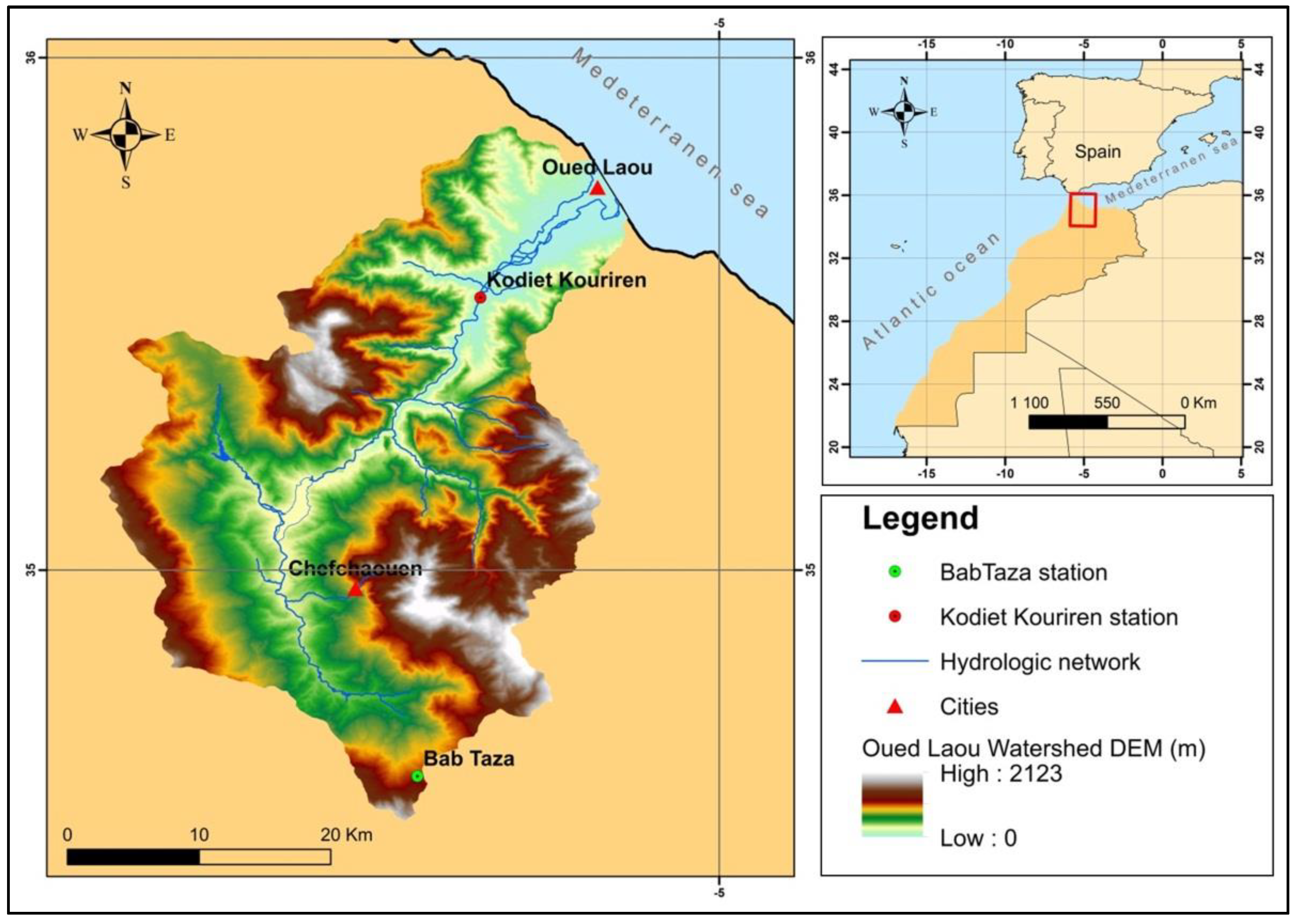
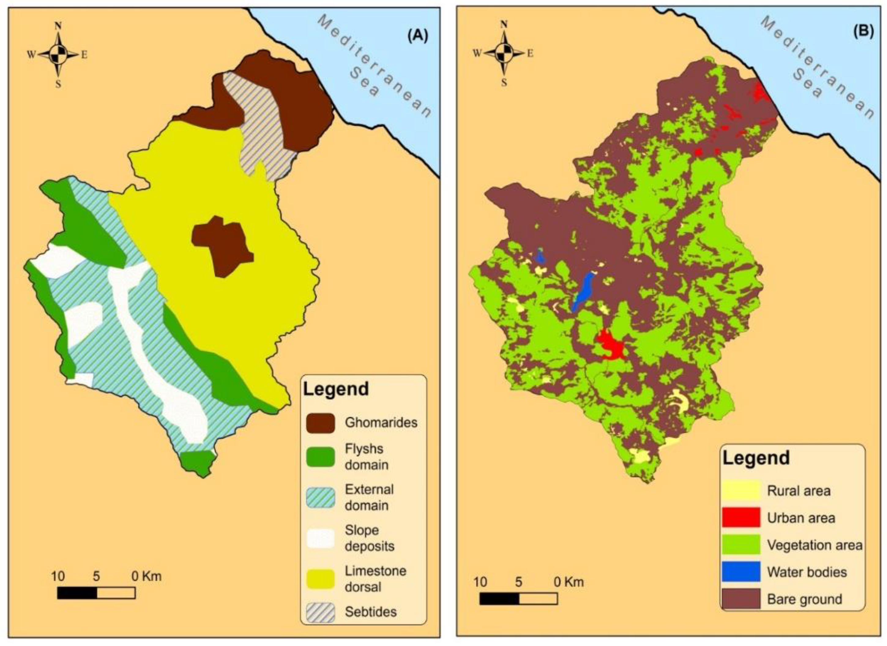
2.1. Description of OLW Area

The OLW (area: 940 km²) is located in the northern part of Morocco (Figure 1). The OLW is surrounded by the summits of Jebel Soukna (elevation: 1800 m above sea level) and Tissouka (2180 m) to the southeast, Jebel Kelti (1928 m) to the west, and Jebel Tazoute (1800 m) to the northeast and the Mediterranean Sea to the north (Figure 1). The OLW is marked by its rugged slopes [36]. In terms of climate, the OLW is stretched over a Mediterranean sub-humid climate zone with high rainfall in winter and hot, dry summers [50].

Precipitation is the highest of all in Morocco [56], reaching up to 1602 mm/year in the southern upstream parts of the OLW and decreasing to 300 mm/year in the northern parts of the watershed (Figure 2).

Geologically, the OLW is characterized by a significant geological diversity given its location in the Rifan Chain; it is composed of formations of the internal domain (limestone ridge and Paleozoic sheet) and external domain and also of flysch sheet or shale (Figure 3A). In terms of permeability, the OLW is covered by impermeable or low-permeability facies, and only the limestone chain, the plains, and the alluvial valleys witness high infiltration [56]. The OLW is occupied by forest and moderately cultivated land (60%) and bare soil (33%), while urban, rural, and water areas occupy 2.46%, 1.78%, and 2.76% of the OLW, respectively (Figure 3B).

2.2. Data

Daily rainfall and streamflow data from 2004 to 2012, which are equivalent to 2920 days, were selected to assess the performance of three hydrological models platforms to continuously simulate streamflow patterns in the OLW. The hydroclimatic data used in this modelling approach mainly consist of precipitation, solar radiation, temperature (max, min, average daily), relative humidity, wind speed, and discharge time series recorded at two rain gauges (Kodiet Kouriren and Bab Taza; Figure 1) and at a streamflow gauge (Kodiet Kouriren; Figure 1). The data used in this project were obtained from the Loukkos Hydraulic Basin Agency in Tetouan. Furthermore, a 12.5 m spatial resolution digital elevation model (DEM) downloaded over the OLW area from the Alaska Satellite Facility was used for the geographic analysis. Land-use data from (www.globallandcover.com, accessed on 1 January 2019) with a 30 m spatial resolution were used for the daily time step as the watershed coverage. The World Soil Database (www.fao.org, accessed on 31 December 2018) was used as the input data for the soil maps.

2.3. Description of Selected Rainfall-Runoff Models

The availability of a wide variety of rainfall-runoff models provides unprecedented opportunities to model the hydrogeologic behaviors of different hydrologic units. However, the model selection is a challenging task. In this context, Melsen et al. [57] have indicated that for an appropriate selection of a hydrological model, the primary need is to clarify the purpose of the study (e.g., water resources management or flood modelling). In the same line of thought, Paul et al. [58] underlined that the selection of an adequate model should be based on its suitability for the research questions comprising the study objective, the spatiotemporal scales, as well as the landscape of the region. In this study, three structurally and physically different hydrological models, namely ATHYS [59], HEC-HMS [60], and SWAT [43], were selected to quantify runoff rates and locations in the OLW and determine the optimal model for assessment of the rainfall-runoff behavior in the OLW and similar watersheds. These models are different in their physics, structures, input/output parameters, and spatial discretization.

2.3.1. HEC-HMS

The HEC-HMS model was developed by the United States (U.S.) Army Corps of Engineers and designed to simulate continuous hydrological processes and flood events [60]. This semi-distributed model has been successfully used worldwide to simulate hydrological processes by different hydrologists [61,62,63,64,65,66].

In this study, the basin model files and meteorological model files were prepared using the HEC-GeoHMS extension tool of Arc-GIS software. The watershed is given as an interconnected system with hydrologic and hydraulic components that are combined to simulate the basin processes. Each component is representative of the factors to convert precipitation to runoff within a part of the basin, which is usually considered as the sub-basin. The SCS-CN (soil conservation service-curve number) production function is used for the estimation of the infiltration and surface drainage process in the Mediterranean watershed [67,68].

$$P_e=\frac{{\left(P-I_a\right)}^2}{P-I_a+S}$$

(1)

where P_e is the excess precipitation, P is the total precipitation, I_a is the initial losses, and S is the maximum retention potential. In the SCS-CN method, the initial losses are given by the relationship I_a = 0.2S. The retention potential S is related to the CN, which in turn can be estimated as a function of hydrologic soil group HSG, land-cover classification, and hydrologic conditions according to USDA and NEH-4 standard lookup tables [69] or by calibration with observed data [70]:

$$S=\frac{\mathrm{254,400}-254 CN}{CN}$$

(2)

The Muskingum–Cunge method was adopted for the representation of the flood propagation process in the water bodies, while the rainfall transformation in runoff was estimated by the SCS Unit Hydrograph method.

In this model, the adopted modelling approach for simulating the hydrological behavior of OLW is a lumped one without spatialization of rainfall, land-use, or soil properties. The SCS-CN function, which is known to be the most sensitive parameter, was selected to be calibrated, while the concentration time parameter of the transfer function was computed and fixed based on an empirical formula. These methods are the most used and appropriate in the Moroccan watersheds [36,37,71]. Details of the underlying principles of the HEC-HMS model can be found in [33].

2.3.2. ATHYS

The ATHYS modelling platform (http://www.athys-soft.org, accessed on 15 January 2019) [72] has been used successfully to reproduce the hydrological behavior of several Mediterranean watersheds [40,73,74]. The ATHYS platform includes a set of spatialized hydrological models associated with hydroclimatic and geographic data processing. Such advantages allowed selecting the coupling model that combines the SCS production function and the lag and route (LR) transfer function. The SCS-LR model is a distributed model with reservoirs based on a discretization of the considered watershed into regular square cells in the Mediterranean watershed. The SCS production function is used to estimate the runoff production of the cell based on the following equation:

$$R\left(t\right)=C\left(t\right).Pb\left(t\right)$$

(3)

where R(t) is the runoff of the cell (mm.h⁻¹), C(t) is a time variable runoff coefficient (%), and Pb(t) is the instantaneous precipitation (mm.h⁻¹).

The cell production is routed to the downstream based on the LR transfer function as follows:

$$q_m\left(t\right)=0 \mathrm{if} \mathrm{t} <t_0+T_m$$

(4)

$$q_m\left(t\right)=\frac{p_e\left(t_0\right)}{K_m}exp\left(-\frac{t-\left(t_0-T_m\right)}{K_m}\right).A \mathrm{if} \mathrm{t}<t_0+T_m$$

(5)

where P_e(t₀) is the effective rainfall of cell (mm) at time to, Tm is propagation time at the outlet (s), Km is a diffusion time (s), A is the cell size (m²), and q(t) is the elementary discharge (m³/s). The complete flood hydrograph is produced by adding up all the contributions of the cells at each time.

In this model, the OLW divided into regular cells with the rainfall information is spatially interpolated based on the Thiessen polygons method. The SCS-LR combined model does not take into account the physical properties of the considered watershed. The S parameter of SCS production function and flow velocity V0 of the LR transfer function were calibrated, while the remaining parameters were set based on the literature values. An extended background on the ATHYS model can be viewed at (http://www.athys-soft.org, accessed on 15 January 2019) [72].

2.3.3. SWAT

SWAT was developed by the United States Department of Agriculture (USDA). It is a physical-based spatially distributed model, which requires specific information related to the watershed’s weather conditions, soil properties, land management, cultural practices, and flows. SWAT, as a semi-distributed model, has been largely used to model runoff, water quality, and sediment in many different watersheds [75,76,77,78,79].

In this model, the simulations are performed on a continuous time scale, and the basin is divided into sub-basins, which are then divided into hydrological response units (HRU). HRU are defined as homogeneous spatial units that have similar hydrological and geomorphological properties [80]. The hydrologic cycle in SWAT is simulated based on the water balance:

$$S{W}_t=S{W}_0+{{\displaystyle \sum }}_{n=1}^t\left(R_{day}-Q_{surf}-E_a-W_{seep}-Q_{gw}\right)$$

(6)

where SW_t refers to the final soil water content (mm), SW₀ refers to the initial soil water content (mm), Rday refers to the amount of precipitation (mm), t is time (days), Q_surf represents the amount of surface runoff (mm), E_a represents the amount of evapotranspiration (mm), Wseep is the amount of water entering the vadose zone from the soil profile (mm), and Q_gw is the amount of return flow (mm).

In SWAT model, the surface runoff is simulated based on the SCS-CN function. The surface flow is routed based on kinematic wave transfer function, while the return flow is predicted assuming a shallow aquifer [81,82,83].

In this model, the OLW is divided into several HRUs. To simulate the hydrological behavior of the studied watershed, SWAT provides us with 28 parameters to set up. The large number of parameters included in the SWAT model makes its parameterizations particularly challenging. A sensitivity analysis was carried out to select sensitive parameters to be included for calibration. After 250 runs, the assessment of sensitivity of 28 different SWAT parameters revealed that six parameters were the most influential: CN (curve number, moisture condition II (dimensionless)); ESCO (soil evaporation compensation factor (dimensionless)); SOL_AWC (available soil moisture capacity, mm h⁻¹); ALPH_BF (base flow recession constant, days); CH_N2 (Manning’s “n” value for the main channel); and CH_K2 (effective hydraulic conductivity in the channel alluvium), which were all identified to be calibrated. A full description of the SWAT model can be found in the literature [38,84].

2.4. Calibration and Validation Procedures and Performance Criteria

The process of model calibration and validation is performed manually by applying the classical split sample test. In this method, the streamflow time series is divided into two sets. The first set (2004 to 2009) is used for the calibration phase and the remaining set (2009 to 2011) for model validation. The median values of calibrated parameters for best fit between observed and estimated streamflow were used for validation.

In all three models, the simulations were performed in continuous mode with a daily time step.

2.5. Performance Criteria

In order to test the performance of the parameterized models and their ability to reproduce the flows at the outlet of the OLW, the modeled flows were assessed using four indices, and their equations are described below:

Nash and Sutcliffe (NSE)

$$NSE=1-\left[\frac{{{\displaystyle \sum }}_{i=1}^n\left(Q_i^{obs}-Q_i^{sim}\right)²}{{{\displaystyle \sum }}_{i=1}^n\left( Q_i^{obs}-Q^{mean}\right)²}\right]$$

(7)

It is estimated that the simulation is of poor quality when the Nash criterion is low (<0.5), it is acceptable when it is greater than (>0.7), and it is perfect when it is equal to (1) [85].

Linear correlation coefficient (R²)

$$R²=\frac{{{\displaystyle \sum }}_{i=1}^n(Q_{obs}-\overline{Q_{obs}})\left(Q_{sim }-\overline{Q_{sim }} \right)}{\sqrt{{{\displaystyle \sum }}_{i=1}^n(Q_{obs}-\overline{Q_{obs }} )²}\sqrt{{{\displaystyle \sum }}_{i=1}^n(Q_{sim }-\overline{Q_{sim }} )²}}$$

(8)

The closer R² is to 1, the closer the result of simulation is to the observation [86].

Root mean square error observations standard deviation ratio (RSR)

To quantify the prediction error in terms of units of the variable computed by the model, we selected the (RSR). It uses observations’ standard deviation (SD) to standardize root mean square error (RMSE). RSR is the ratio of the RMSE and SD of observed data. This is a frequently used indicator and its definition is as follows:

$$RSR=\sqrt{\frac{{{\displaystyle \sum }}_{i=1}^N{(Q_i^{obs}-Q_i^{sim})}^2}{{{\displaystyle \sum }}_{i=1}^N{(Q_i^{obs}-Q_{ave}^{obs})}^2}}$$

(9)

where $Q_i^{sim}$ and $Q_i^{obs}$ are the sample (of size N) containing the model estimates and the observations, respectively. It ranges from 0 to +∞, where RSR = 0 indicates a perfect fit [87].

Percent bias coefficient (PBIAS)

$$PBIAS=\left[\frac{{{\displaystyle \sum }}_{i=1}^n\left(Q_i^{obs}-Q_i^{sim}\right)\times \left(100\right)}{{{\displaystyle \sum }}_{i=1}^n\left(Q_i^{obs}\right)}\right]$$

(10)

The optimum value is 0.0, with values of low magnitude denoting accurate simulation of the model. A positive value denotes model overestimation bias, and negative values denote model underestimation bias. It is useful for continuous long-term simulations and can help identify average model simulation bias (over prediction vs. under prediction) and can incorporate measurement uncertainty [88].

Here, $Q_i^{obs} \mathrm{and} Q_i^{sim}$ are the observed and estimated flow, respectively; n is the number of data points; and ${\mathrm{Q}}^{\mathrm{mean}}$ is the mean of the observed flow peak over the investigated period.

It is significant to consider that the performance of the evaluation criteria differs depending on the targeted portion (peak, medium, and low flows) of the hydrograph [60].

3. Results and Discussion

In this study, the overall performance and robustness of the three models were assessed by analyzing the physical meaning of calibrated parameters and evaluating models performances in the calibration and validation periods.

3.1. Optimized Values of Calibrated Parameters

The optimized values of calibrated parameters for each model are shown in

Table 1. Calibrated parameter median values for the three models.

Model	Calibrated Parameters	Parameters Names	Values	Parameter Range
HEC-HMS	CN (dimensionless)	Curve number, moisture condition II	75	(69.8–93.0)
	Lag (min)	Lag time	4.5
ATHYS	CN (dimensionless)	Curve number, moisture condition II	73.57	(69.8–93.0)
	ds (1/day)	Drainage coefficient f(t) infiltration	0.12	-
	VO (m/s)	Flow velocity	1.80	-
	S (mm/mm)	Soil reservoir capacity (the potential maximum retention)	91.25	(0–+∞)
SWAT	CN2 (dimensionless)	Curve number, moisture condition II	74	(69.8–93.0)
	ESCO (dimensionless)	Soil evaporation compensation factor	0.83	(0.01–1)
	SOL_AWC (mm/mm)	Available soil moisture capacity, mm h −1	0.4	(−0.6 to 0.6)
	ALPHA_BF (1/day)	Base flow recession constant, days	0.43	(0–0.048)
	CH_N2 (s/m1/3)	Manning’s “n” value for the main channel	0.15	(0.01–0.25)
	CH_k2 (mm/h)	Effective hydraulic conductivity in the channel alluvium	58	(0–150)

. The number of sensitive parameters increases with increasing model complexity (2 for HEC-HMS, 4 for ATHYS, and 6 for SWAT). In this sense, the CN parameter showed a significant impact on the simulated flow in all three models, which confirms that the land-use and soil parameters have a significant influence on the hydrological simulations. The CN values are approximately equal in the SWAT, HEC-HMS, and ATHYS models, with calibrated values of 74, 75 and 73, 57, respectively (Table 1).

The values of the calibrated parameters in the HEC-HMS model may be related to the fact that the model was designed to consider fixed values for the physical parameters during the simulation period (CN, Lag, and Ia); however, land-use changes resulting from human activities sometimes lead to uncertainty in the CN. In addition, the CN method was originally designed for a temperate regime.

The sensitivity analysis revealed that the efficiency of the ATHYS model depends mainly on three parameters: S, ds, and V0. The S variable relies on several factures of the impermeable layer of the roads and urban regions, and changing these variables leads to the increase of the flows at the outlets [41,79].

The SWAT model employs certain parameters that the HEC-HMS and ATHYS models do not take into account (Table 1). However, the structure of the SWAT model is more complex than that of ATHYS, which is a bit complex when compared with the HEC-HMS model. This difference in complexity may raise the uncertainty of the modeled streamflow outputs. Among the six SWAT model parameters shown in (Table 1), the initial SCS-CN was found to be the most sensitive. Despite SWAT being a physical-based model, certain processes are represented by empirical functions, such as the runoff, and for this reason, the CN was quite important during simulation. The sensitivity analysis allowed decreasing the number of parameters to be calibrated for the SWAT model, which enabled avoiding the problem of over parameterization and improvement of the results of the simulations.

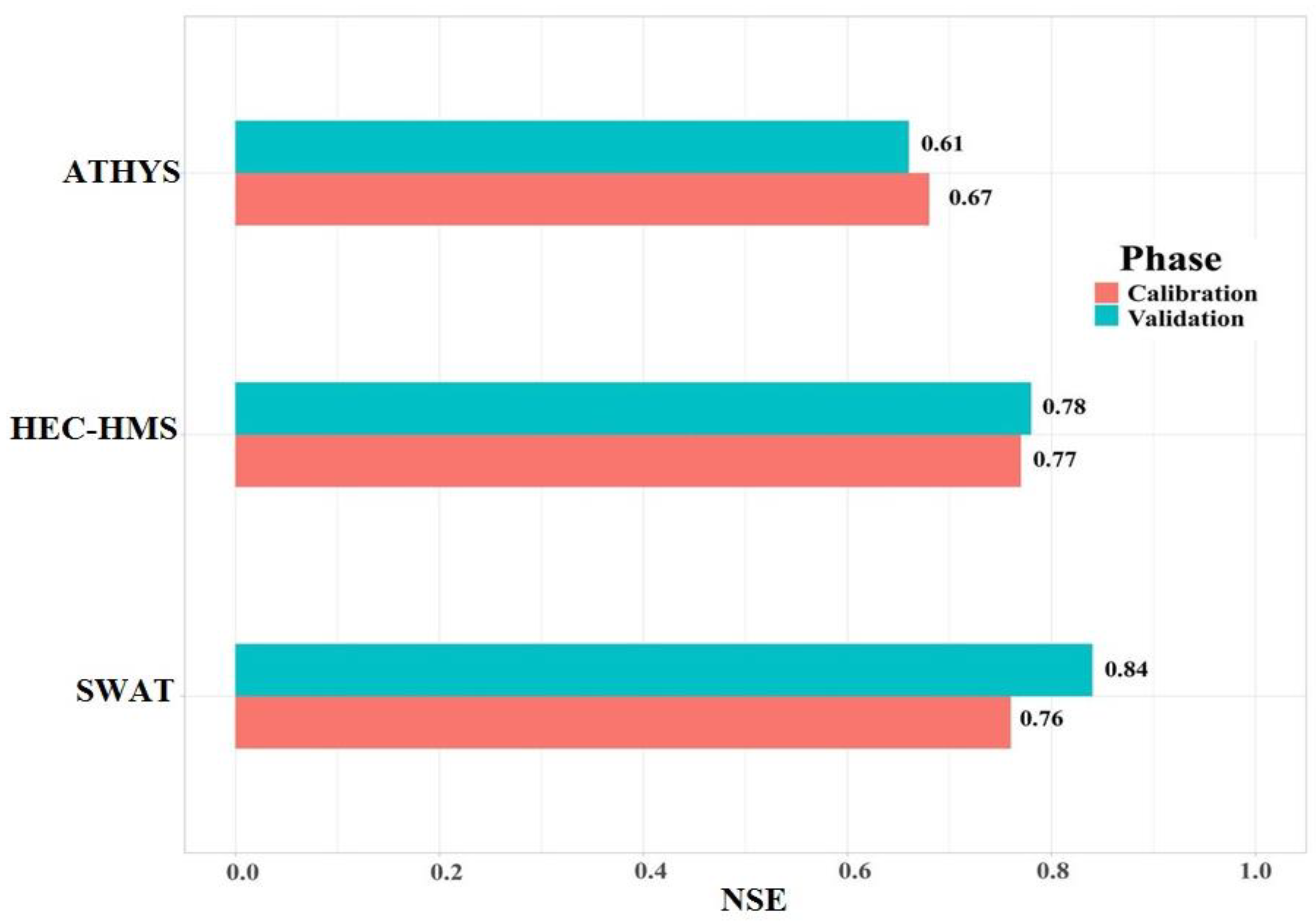
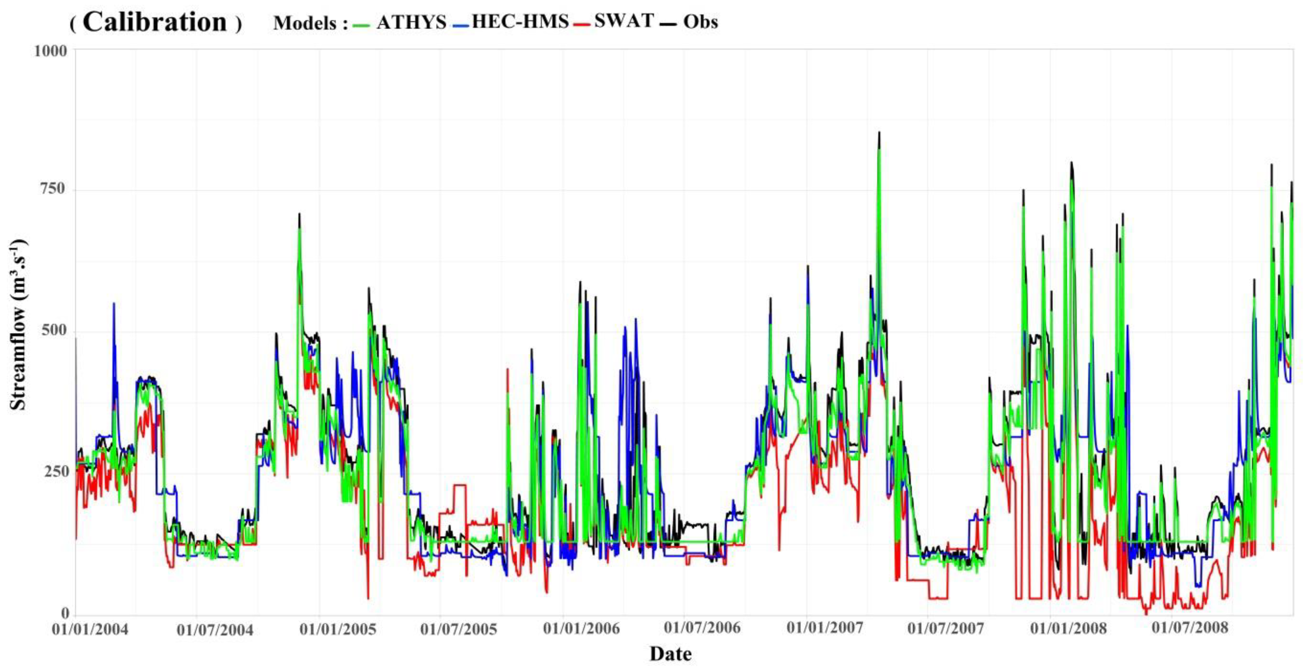
3.2. Analysis of the Calibration and Validation Performances

The NSE of the SWAT-derived runoff during the validation phase is higher than that of HEC-HMS and ATHYS (Figure 4). During the calibration phase, the Nash–Sutcliff coefficients of HEC-HMS and SWAT are approximately the same, while during the validation, a good improvement is detected in the Nash–Sutcliff coefficient of SWAT, which reaches 0.84. A minor Nash–Sutcliff coefficient improvement is detected in the validation phase of the HEC-HMS model, while the ATHYS model shows a decrease in performance from 0.67 during the calibration period to 0.61 during the validation period, which might be related to the structure and concept of the model. The inter-comparison of the three models shows a clear improvement in terms of discharge restitution when moving from calibration to validation for the SWAT and HEC HMS models (Figure 4).

The SWAT model performs well (NSE = 0.76) over both periods, with an improvement of 0.08 in validation. A good agreement can be observed in the HEC-HMS model outputs, with an approximately stable NSE of 0.77 and 0.78 for the calibration and validation phases, respectively. The coefficient of determination (R²) and scatterplots for all models are shown in (Figure 5). The results of the linear correlation of simulated discharge in the ATHYS model show an R² of 0.68 during the calibration with a decrease of 0.02 towards the validation. The observed drop in the ATHYS model performance based on R² and NSE criteria in the validation phase reveals that it is the least adapted to the particularities of the study area.

The results of the other performances criteria, namely RSR and PBIAS (

Table 2. RSR and PBIAS values for the calibration and validation periods.

Model	RSR		PBIAS
	Calibration	Validation	Calibration	Validation
HEC-HMS	0.53	0.51	15%	14%
ATHYS	0.51	0.53	14%	16%
SWAT	0.52	0.41	12%	9%

), confirm the findings mentioned above. The performance criteria show good results; however, they differ significantly. The SWAT model underestimates the discharge. This could be due to the fact that SWAT-derived lateral discharge relies on the relative slope, and the OLW possesses a relatively steep slope. Therefore, we may argue that the SWAT model underestimates the flow in the steep slope area in OLW. This deficiency leads to a surface runoff fraction of nearly 35% in OLW, as surface runoff and base flow compensate for the missing interflow. Soil characteristics, particularly hydraulic conductivity data, create uncertainty and cause problems in representing infiltration characteristics correctly.

Examination of Table 2 indicates that the ATHYS does not manage to improve the simulation in the validation phase, contrary to HEC-HMS and SWAT, which show a certain improvement in this phase by reduction in residue error, especially in the SWAT model. (RSR decreases from 0.52 in calibration to 0.41 in validation.)

The ATHYS model exhibits some prediction uncertainties in the simulations and in the discharge estimate. It can be observed that simply introducing more realistic soil characteristics improves the simulation, increasing the high flow peaks, especially in the driest seasons where low flow decreases in a more realistic simulation. In the ATHYS model, the continuous mode simulation is very time-consuming compared to other models (e.g., SWAT and HEC-HMS). The performance of the HEC-HMS model for both simulation periods indicates a positive trend with a small improvement in validation. In the HEC-HMS model, the watershed is presented as an interconnected system with hydrologic and hydraulic components. Several components are combined to simulate processes in the watershed; each component is representative of the factors that convert precipitation to runoff in parts of the watershed that are usually considered sub-basins. The graphical results show that the HEC-HMS model gives better results for the OLW.

The graphic comparison of the model-derived discharge allows the identification of possible sources of uncertainty in the hydrological modelling of the OLW. Figure 6 shows the difference between observed and measured streamflow for the three models (e.g., SWAT, ATHYS, and HEC-HMS) during calibration and validation phases.

The HEC-HMS model overestimates the discharge at the beginning of the calibration period, and it underestimates the discharge towards the end of the simulation during the calibration and during the validation period (Figure 6).

Despite the fact that the SWAT model underestimated the base flow, this model perfectly reproduces the observed hydrograph in term of peak flows on the OLW (Figure 6).

The ATHYS model gave satisfactory results for the two simulation periods in the studied watershed. The model underestimates the observed flow at the beginning of the calibration and overestimates the flow in the middle and towards the end of the calibration; from the graphical analysis, we can notice that the model oscillates between underestimating and overestimating of the discharge during the calibration and validation period (Figure 6).

The maximum simulated flows are often underestimated by the three models. The majority of hydrologists agree that underestimation of rainfall measurements is the main driver of uncertainty [89,90,91]. The results obtained for the three model platforms are relatively good. These results reinforced the multi-functionality and reliability of these three models as relevant tools for the management and control of water resources in Morocco.

3.3. Detailed Discussion on Models’ Performance

An overview of the performance of the three models was provided to verify which of them is most applicable to the study area. Figure 4 shows that the SWAT model performs best in terms of the NSE criterion, especially during the validation period, with the other performance criteria (R², PBIAS, and RSR) showing the same results. According to the results presented by Shekar and Vinay [92] in a sub-humid tropical watershed, SWAT performed better then HEC-HMS, while a study in the Ethiopian Rift Valley lake basin comparing HEC-HMS with the SWAT model found contradictory results [93]: they found an increase in the performance of the HEC-HMS model in the validation period, and they found that the results provided by the HEC-HMS model are more satisfactory than those provided by the SWAT model. From our results and these studies, we could see that the performance of these models relies on the soil type, elevation, and other characteristics of the watershed. The SWAT model uses characteristics such as soil type, land-use and cover, and slope, which influence the characteristics of the flow of a watershed, minimum temperature, solar radiation, precipitation, relative temperature, humidity, and wind speed for modelling various physical processes. Although the models of the SWAT platform give us good results in simulations, SWAT proves to be more adapted to the simulation of continuous scenarios of large scales of time (more than 30 years) because SWAT requires a great deal of input data. This model can be used in the OLW to study the phenomena of water erosion caused by deforestation and flash floods. SWAT can also be used for futuristic prediction of climate change, land use and land cover, and other watershed management scenarios [38].

The HEC-HMS model presents good result in the two simulations periods, similar to SWAT, while the HEC-HMS model fails to correctly estimate peak flows although the overall performance is better. The HEC-HMS model is less demanding than the SWAT model in terms of input data for runoff calibration, and the simulation results are very good; after taking into account all types of uncertainties during the model input and daily parameterization process, better correlation and good agreement between the measured data and the estimated daily flow data were shown. During the application, it is observed that the modelling procedure by HEC-HMS platform is flexible; however, some appropriate ground measurements and analysis can be used to improve the simulation results.

The most noticeable distinctions between the HEC-HMS and SWAT and ATHYS models are several properties described as follows: The HEC-HMS and SWAT models are treated as semi-distributed models that spatially interpolate rainfall inputs, and ATHYS is processed as a spatially distributed model. The simulated runoff differs between them probably due to the complexity of the model and the rationality of the parameterization. The reason for the greater uncertainty in model calibration and validation observed for ATHYS compared to SWAT and HEC-HMS can be explained by the complexity of the model structure.

The results show that the simulated peak flows are underestimated for the majority of the simulation periods, and the origin of this underestimation is probably related to the underestimation of rainfall, which is marked by significant spatial heterogeneity, which therefore represents the main difficulties in quantifying rainfall. The heterogeneity of rainfall was demonstrated by the observations of [94], who found that the more pronounced the rainfall intensity is, the smaller the affected area will be [95], confirming that the runoff production and hydrological process in a watershed are strongly influenced by the spatial variability of rainfall. Bouizrou et al. [41] demonstrated that the performance of the ATHYS model was higher when precipitation information was obtained from multiple rain gauges, suggesting that additional knowledge of the spatial variability of precipitation can improve model performance.

The difference between the coefficient of determination and the Nash–Sutcliffe coefficient for the three models is due to the underestimation of peak flows by SWAT model, underestimates in the major phases by HEC-HMS, and fluctuations between underestimation and overestimation of flow by the ATHYS model.

The advantages and limitations of these three models remain to be explored in more comprehensive applications. As discussed here, they hold considerable promise for meeting important contemporary challenges, for characterizing OLW diversity, and more widely for helping to move toward a more unified watershed-scale hydrologic theory. We emphasize that the generation and testing of multiple model alternatives must be carefully controlled. It is equally critical to avoid “over-fitting” a model setup.

4. Conclusions

In this study, we examined three rainfall-runoff patterns in the OLW located in northern Morocco. Daily rainfall data for 4 years (2004–2008) were used for calibration and 3 years (2009–2011) to validate the three structurally and physically different hydrological models. The multi-criteria model comparison shows that all three models are capable of reproducing the observed flows at calibration and validation phases. The SWAT model performs well over both periods, with an improvement in validation, which confirms its applicability in the sub-humid context. Furthermore, a good agreement can be observed in the HEC-HMS model outputs, with an approximately stable R² = 0.82 during the two simulation periods, while the ATHYS model shows a decrease in performance from 0.67 in the calibration period to 0.61 in the validation period, which might be related to the structure and concept of the model.

The precision of the three hydrological models used in simulation depends on the accuracy of the precipitation, land-use, and soil parameters. Therefore, a detailed spatial distribution and good quality of data measurements are necessary to obtain more accurate hydrological model results. However, rain gauges are scarce and unevenly distributed in the OLW due to financial and other technological constraints. However, we propose to implement more accurate estimates of surface precipitation and rain gauge stations in the near future in order to obtain specific hydrological models for the OLW. As a result, in this study, SWAT and HEC-HMS are the most appropriate models for OLW rainfall-runoff simulation because they have the best compromise between parameterization efforts and physical representativeness, followed by ATHYS.

References

1. Hong, X.; Guo, S.; Chen, G.; Guo, N.; Jiang, C. A Modified Two-Parameter Monthly Water Balance Model for Runoff Simulation to Assess Hydrological Drought. Water 2022, 14, 3715. [Google Scholar] [CrossRef]
2. Shigute, M.; Alamirew, T.; Abebe, A.; Ndehedehe, C.E.; Kassahun, H.T. Understanding Hydrological Processes under Land Use Land Cover Change in the Upper Genale River Basin, Ethiopia. Water 2022, 14, 3881. [Google Scholar] [CrossRef]
3. Rueda, V.; Young, M.H.; Faust, K.; Rateb, A.; Leibowicz, B.D. System Dynamics Modeling in Local Water Management: Assessing Strategies for the City of Boerne, Texas. Water 2022, 14, 3682. [Google Scholar] [CrossRef]
4. Mendez, M.; Calvo-Valverde, L.-A.; Imbach, P.; Maathuis, B.; Hein-Grigg, D.; Hidalgo-Madriz, J.-A.; Alvarado-Gamboa, L.-F. Hydrological Response of Tropical Catchments to Climate Change as Modeled by the GR2M Model: A Case Study in Costa Rica. Sustainability 2022, 14, 16938. [Google Scholar] [CrossRef]
5. Rufino, P.R.; Gücker, B.; Faramarzi, M.; Boëchat, I.G.; Cardozo, F.D.S.; Santos, P.R.; Zanin, G.D.; Mataveli, G.; Pereira, G. Evaluation of the SWAT Model for the Simulation of Flow and Water Balance Based on Orbital Data in a Poorly Monitored Basin in the Brazilian Amazon. Geographies 2022, 3, 1–18. [Google Scholar] [CrossRef]
6. Janicka, E.; Kanclerz, J. Assessing the Effects of Urbanization on Water Flow and Flood Events Using the HEC-HMS Model in the Wirynka River Catchment, Poland. Water 2022, 15, 86. [Google Scholar] [CrossRef]
7. Rocha, J.; Duarte, A.; Fabres, S.; Quintela, A.; Serpa, D. Influence of DEM Resolution on the Hydrological Responses of a Terraced Catchment: An Exploratory Modelling Approach. Remote Sens. 2022, 15, 169. [Google Scholar] [CrossRef]
8. Van, S.P.; Le, H.M.; Thanh, D.V.; Dang, T.D.; Loc, H.H.; Anh, D.T. Deep learning convolutional neural network in rainfall–runoff modelling. J. Hydroinforma. 2020, 22, 541–561. [Google Scholar] [CrossRef] [Green Version]
9. Deb, P.; Kiem, A.S. Evaluation of rainfall–runoff model performance under non-stationary hydroclimatic conditions. Hydrol. Sci. J. 2020, 65, 1667–1684. [Google Scholar] [CrossRef]
10. Dubovský, V.; Dlouhá, D.; Pospíšil, L. The Calibration of Evaporation Models against the Penman–Monteith Equation on Lake Most. Sustainability 2020, 13, 313. [Google Scholar] [CrossRef]
11. Paniconi, C.; Putti, M. Physically based modeling in catchment hydrology at 50: Survey and outlook. Water Resour. Res. 2015, 51, 7090–7129. [Google Scholar] [CrossRef] [Green Version]
12. Ouermi, K.S.; Paturel, J.-E.; Adounpke, J.; Lawin, A.E.; Goula, B.T.A.; Amoussou, E. Comparison of hydrological models for use in climate change studies: A test on 241 catchments in West and Central Africa. Comptes Rendus Geosci. 2019, 351, 477–486. [Google Scholar] [CrossRef]
13. Archfield, S.A.; Clark, M.P.; Arheimer, B.; Hay, L.E.; McMillan, H.; Kiang, J.E.; Seibert, J.; Hakala-Assendelft, K.; Bock, A.; Wagener, T.; et al. Accelerating advances in continental domain hydrologic modeling. Water Resour. Res. 2015, 51, 10078–10091. [Google Scholar] [CrossRef] [Green Version]
14. Xu, T.; Liang, F. Machine learning for hydrologic sciences: An introductory overview. WIREs Water 2021, 8, e1533. [Google Scholar] [CrossRef]
15. KlemeŠ, V. Operational Testing of Hydrological Simulation Models. Hydrol. Sci. J. 1986, 31, 13–24. [Google Scholar] [CrossRef]
16. Ewen, J.; Parkin, G. Validation of Catchment Models for Predicting Land-Use and Climate Change Impacts. 1. Method. J. Hydrol. 1996, 175, 583–594. [Google Scholar] [CrossRef]
17. Wood, A.; Leung, L.R.; Sridhar, V.; Lettenmaier, D.P. Hydrologic Implications of Dynamical and Statistical Approaches to Downscaling Climate Model Outputs. Clim. Chang. 2004, 62, 189–216. [Google Scholar] [CrossRef]
18. Fowler, H.J.; Blenkinsop, S.; Tebaldi, C. Linking Climate Change Modelling to Impacts Studies: Recent Advances in Downscaling Techniques for Hydrological Modelling. Int. J. Climatol. 2007, 27, 1547–1578. [Google Scholar] [CrossRef]
19. Rosero, E.; Yang, Z.-L.; Wagener, T.; Gulden, L.E.; Yatheendradas, S.; Niu, G.-Y. Quantifying Parameter Sensitivity, Interaction, and Transferability in Hydrologically Enhanced Versions of the Noah Land Surface Model over Transition Zones during the Warm Season. J. Geophys. Res. 2010, 115. [Google Scholar] [CrossRef] [Green Version]
20. Merz, R.; Parajka, J.; Blöschl, G. Time Stability of Catchment Model Parameters: Implications for Climate Impact Analyses. Water Resour. Res. 2011, 47, 1–17. [Google Scholar] [CrossRef]
21. Seiller, G.; Anctil, F.; Perrin, C. Multimodel Evaluation of Twenty Lumped Hydrological Models under Contrasted Climate Conditions. Hydrol. Earth Syst. Sci. 2012, 16, 1171–1189. [Google Scholar] [CrossRef] [Green Version]
22. Gharari, S.; Hrachowitz, M.; Fenicia, F.; Savenije, H.H.G. An Approach to Identify Time Consistent Model Parameters: Sub-Period Calibration. Hydrol. Earth Syst. Sci. 2013, 17, 149–161. [Google Scholar] [CrossRef] [Green Version]
23. Coron, L.; Andréassian, V.; Perrin, C.; Bourqui, M.; Hendrickx, F. On the Lack of Robustness of Hydrologic Models Regarding Water Balance Simulation: A Diagnostic Approach Applied to Three Models of Increasing Complexity on 20 Mountainous Catchments. Hydrol. Earth Syst. Sci. 2014, 18, 727–746. [Google Scholar] [CrossRef] [Green Version]
24. Ewert, F.; Rötter, R.P.; Bindi, M.; Webber, H.; Trnka, M.; Kersebaum, K.C.; Olesen, J.E.; van Ittersum, M.K.; Janssen, S.; Rivington, M.; et al. Crop Modelling for Integrated Assessment of Risk to Food Production from Climate Change. Environ. Model. Softw. 2015, 72, 287–303. [Google Scholar] [CrossRef]
25. Dakhlaoui, H.; Ruelland, D.; Tramblay, Y.; Bargaoui, Z. Evaluating the Robustness of Conceptual Rainfall-Runoff Models under Climate Variability in Northern Tunisia. J. Hydrol. 2017, 550, 201–217. [Google Scholar] [CrossRef]
26. Wilby, R.L.; Dessai, S. Robust Adaptation to Climate Change. Weather 2010, 65, 180–185. [Google Scholar] [CrossRef] [Green Version]
27. Tramblay, Y.; Ruelland, D.; Somot, S.; Bouaicha, R.; Servat, E. High-Resolution Med-CORDEX Regional Climate Model Simulations for Hydrological Impact Studies: A First Evaluation of the ALADIN-Climate Model in Morocco. Hydrol. Earth Syst. Sci. 2013, 17, 3721–3739. [Google Scholar] [CrossRef] [Green Version]
28. Jaber, F.H.; Shukla, S. MIKE SHE: Model use, calibration, and validation. Trans. ASABE 2012, 55, 1479–1489. [Google Scholar] [CrossRef]
29. Bergström, S. The HBV model. Comput. Model. Watershed Hydrol. 1995, 443–476–476. [Google Scholar]
30. Lindström, G.; Pers, C.; Rosberg, J.; Strömqvist, J.; Arheimer, B. Development and testing of the HYPE (Hydrological Predictions for the Environment) water quality model for different spatial scales. Hydrol. Res. 2010, 41, 295–319. [Google Scholar] [CrossRef]
31. Markstrom, S.L.; Regan, R.S.; Hay, L.E.; Viger, R.J.; Webb, R.M.; Payn, R.A.; LaFontaine, J.H. PRMS-IV, the precipitation-runoff modeling system, version 4. US Geol. Surv. Tech. Methods 2015, 6, B7. [Google Scholar]
32. Akoko, G.; Le, T.; Gomi, T.; Kato, T. A Review of SWAT Model Application in Africa. Water 2021, 13, 1313. [Google Scholar] [CrossRef]
33. Halwatura, D.; Najim, M. Application of the HEC-HMS model for runoff simulation in a tropical catchment. Environ. Model. Softw. 2013, 46, 155–162. [Google Scholar] [CrossRef]
34. Bouvier, C.; DelClaux, F. ATHYS: A hydrological environment for spatial modelling and coupling with GIS. Appl. GIS Hydrol. Water Resour. Manag. 1996, 235, 572–582. [Google Scholar]
35. Yang, S.; Tan, M.L.; Song, Q.; He, J.; Yao, N.; Li, X.; Yang, X. Coupling SWAT and Bi-LSTM for improving daily-scale hydro-climatic simulation and climate change impact assessment in a tropical river basin. J. Environ. Manag. 2023, 330, 117244. [Google Scholar] [CrossRef] [PubMed]
36. Aqnouy, M.; Stitou El Massari, J.E.; Bouadila, A.; Bouizrou, I.; Aoulad Mansour, M.R. Application of Hydrological Model “HEC HMS” In a Mediterranean Watershed (Oued Laou, Northern of Morocco). Int. J. Innov. Appl. Stud. 2018, 24, 1773–1781. [Google Scholar]
37. Faouzi, E.; Arioua, A.; Hssaisoune, M.; Boudhar, A.; Elaloui, A.; Karaoui, I. Sensitivity analysis of CN using SCS-CN approach, rain gauges and TRMM satellite data assessment into HEC-HMS hydrological model in the upper basin of Oum Er Rbia, Morocco. Model. Earth Syst. Environ. 2022, 8, 4707–4729. [Google Scholar] [CrossRef]
38. Aqnouy, M.; El Messari, J.E.S.; Ismail, H.; Bouadila, A.; Navarro, J.G.M.; Loubna, B.; Mansour, M.R.A. Assessment of the SWAT Model and the Parameters Affecting the Flow Simulation in the Watershed of Oued Laou (Northern Morocco). J. Ecol. Eng. 2019, 20, 104–113. [Google Scholar] [CrossRef]
39. Ouallali, A.; Briak, H.; Aassoumi, H.; Beroho, M.; Bouhsane, N.; Moukhchane, M. Hydrological foretelling uncertainty evaluation of water balance components and sediments yield using a multi-variable optimization approach in an external Rif’s catchment. Morocco. Alex. Eng. J. 2020, 59, 775–789. [Google Scholar] [CrossRef]
40. Aqnouy, M.; El Messari, J.E.S.; Bouadila, A.; Morabbi, A.; Benaabidate, L.; Al-Djazouli, M.O. Modeling of Continuous and Extreme Hydrological Processes Using Spatially Distributed Models Mercedes, Vicair and Vishyr in a Mediterranean Watershed. Ecol. Eng. Environ. Technol. 2021, 22, 9–23. [Google Scholar] [CrossRef]
41. Bouizrou, I.; Chahinian, N.; Perrin, J.L.; Müller, R.; Rais, N. Network Representation in Hydrological Modelling on Urban Catchments in Data-Scarce Contexts: A Case Study on the Oued Fez Catchment (Morocco). J. Hydrol. Reg. Stud. 2021, 34. [Google Scholar] [CrossRef]
42. Abdelmounim, B.; Benaabidate, L.; Bouizrou, I.; Aqnouy, M. Implementation of Distributed Hydrological Modeling in a Semi-Arid Mediterranean Catchment “Azzaba, Morocco”. J. Ecol. Eng. 2019, 20, 236–254. [Google Scholar] [CrossRef]
43. Arnold, J.G.; Srinivasan, R.; Muttiah, R.S.; Williams, J.R. Large area hydrologic modeling and assessment part I: Model development 1. JAWRA J. Am. Water Resour. Assoc. 1998, 34, 73–89. [Google Scholar] [CrossRef]
44. CARD. SWAT Literature Database for Peer-Reviewed Journal Articles. 2019. Available online: https://www.card.iastate.edu/swat_articles/ (accessed on 31 December 2018).
45. Perrin, C.; Michel, C.; Andréassian, V. Does a Large Number of Parameters Enhance Model Performance? Comparative Assessment of Common Catchment Model Structures on 429 Catchments. J. Hydrol. 2001, 242, 275–301. [Google Scholar] [CrossRef]
46. Perrin, C.; Michel, C.; Andréassian, V. Improvement of a Parsimonious Model for Streamflow Simulation. J. Hydrol. 2003, 279, 275–289. [Google Scholar] [CrossRef]
47. Bormann, H.; Breuer, L.; Gräff, T.; Huisman, J.A. Analysing the Effects of Soil Properties Changes Associated with Land Use Changes on the Simulated Water Balance: A Comparison of Three Hydrological Catchment Models for Scenario Analysis. Ecol. Model. 2007, 209, 29–40. [Google Scholar] [CrossRef]
48. Gao, C.; Yao, M.T.; Wang, Y.J.; Zhai, J.Q.; Buda, S.; Fischer, T.; Zeng, X.F.; Wang, W.P. Hydrological Model Comparison and Assessment: Criteria from Catchment Scales and Temporal Resolution. Hydrol. Sci. J. 2016, 61, 1941–1951. [Google Scholar] [CrossRef] [Green Version]
49. Koch, J.; Cornelissen, T.; Fang, Z.; Bogena, H.; Diekkrüger, B.; Kollet, S.; Stisen, S. Inter-Comparison of Three Distributed Hydrological Models with Respect to Seasonal Variability of Soil Moisture Patterns at a Small Forested Catchment. J. Hydrol. 2016, 533, 234–249. [Google Scholar] [CrossRef]
50. Stitou Messari, J. Aplicación Del Método DRASTIC Para Evaluar La Vulnerabilidad a La Contaminación Del Acuífero de Oued Laou (Marruecos). Geogaceta 2006, 41, 191–194. [Google Scholar]
51. Qadem, Z.; Obda, K.; Qadem, A.; Lasri, M.; Bouizrou, I. Contribution of the GIS in Terms of Knowledge of the Situation of the Water Resources of the Plain of Saïs Fez and Its Middle Atlasic Borders—Morocco: Aspects, Methods and Quantification of Water Resources. In Geospatial Technology; Springer: Cham, Switzerland, 2020; pp. 83–94. [Google Scholar]
52. Amellah, O.; El Morabiti, K.; Al-Djazouli, M.O. Spatialization and assessment of flood hazard using 1D numerical simulation in the plain of Oued Laou (north Morocco). Arab. J. Geosci. 2020, 13, 635. [Google Scholar] [CrossRef]
53. Serur, A.B. Modeling blue and green water resources availability at the basin and sub-basin level under changing climate in the Weyb River basin in Ethiopia. Sci. Afr. 2020, 7, e00299. [Google Scholar] [CrossRef]
54. Guiamel, I.A.; Lee, H.S. Watershed Modelling of the Mindanao River Basin in the Philippines Using the SWAT for Water Resource Management. Civ. Eng. J. 2020, 6, 626–648. [Google Scholar] [CrossRef] [Green Version]
55. Fels, A.E.A.E.; Alaa, N.; Bachnou, A. Modelling of flood propagation in a semi-arid environment case of the N’FIS basin—Moroccan Western high atlas. Sci. Afr. 2020, 7, e00306. [Google Scholar] [CrossRef]
56. Bouizrou, I.; Aqnouy, M.; Bouadila, A. Spatio-temporal analysis of trends and variability in precipitation across Morocco: Comparative analysis of recent and old non-parametric methods. J. Afr. Earth Sci. 2022, 196, 104691. [Google Scholar] [CrossRef]
57. Melsen, L.A.; Addor, N.; Mizukami, N.; Newman, A.J.; Torfs, P.J.J.F.; Clark, M.P.; Uijlenhoet, R.; Teuling, A.J. Mapping (Dis)Agreement in Hydrologic Projections. Hydrol. Earth Syst. Sci. 2018, 22, 1775–1791. [Google Scholar] [CrossRef]
58. Paul, P.K.; Zhang, Y.; Ma, N.; Mishra, A.; Panigrahy, N.; Singh, R. Selecting hydrological models for developing countries: Perspective of global, continental, and country scale models over catchment scale models. J. Hydrol. 2021, 600, 126561. [Google Scholar] [CrossRef]
59. Bouvier, C.; Fuentes, G.; Dominguez, R. MERCEDES: Un Modèle Hydrologique d’analyse et de Prévision de Crues En Milieu Hétérogène. Crues et inondations. 23emes journées de l’hydraulique. In Proceedings of the Congrès de la Société Hydrotechnique de France, Nîmes France, 14–16 September 1994; Volume 23, pp. 257–260. [Google Scholar]
60. Feldman, A.D. Hydrologic Modeling System HEC-HMS, Technical Reference Manual; U.S. Army Corps of Engineers, Hydrologic Engineering Center, HEC: Davis, CA, USA, 2000.
61. Abushandi, E.; Merkel, B. Modelling Rainfall Runoff Relations Using HEC-HMS and IHACRES for a Single Rain Event in an Arid Region of Jordan. Water Resour. Manag. 2013, 27, 2391–2409. [Google Scholar] [CrossRef]
62. Lehbab-Boukezzi, Z.; Boukezzi, L.; Errih, M. Uncertainty analysis of HEC-HMS model using the GLUE method for flash flood forecasting of Mekerra watershed, Algeria. Arab. J. Geosci. 2016, 9, 751. [Google Scholar] [CrossRef]
63. brahim-Bathis, K.; Ahmed, S.A. Rainfall-runoff modelling of Doddahalla watershed—An application of HEC-HMS and SCN-CN in ungauged agricultural watershed. Arab. J. Geosci. 2016, 9, 170. [Google Scholar] [CrossRef]
64. Ramly, S.; Tahir, W. Application of HEC-GeoHMS and HEC-HMS as Rainfall–Runoff Model for Flood Simulation. In ISFRAM; Springer: Singapore, 2016; pp. 181–192. [Google Scholar] [CrossRef]
65. Wijayarathne, D.B.; Coulibaly, P. Identification of hydrological models for operational flood forecasting in St. John’s, Newfoundland, Canada. J. Hydrol. Reg. Stud. 2020, 27, 100646. [Google Scholar] [CrossRef]
66. Hamdan, A.; Almuktar, S.; Scholz, M. Rainfall-Runoff Modeling Using the HEC-HMS Model for the Al-Adhaim River Catchment, Northern Iraq. Hydrology 2021, 8, 58. [Google Scholar] [CrossRef]
67. Aronica, G.; Candela, A. Derivation of flood frequency curves in poorly gauged Mediterranean catchments using a simple stochastic hydrological rainfall-runoff model. J. Hydrol. 2007, 347, 132–142. [Google Scholar] [CrossRef]
68. Kastridis, A.; Stathis, D. Evaluation of Hydrological and Hydraulic Models Applied in Typical Mediterranean Ungauged Watersheds Using Post-Flash-Flood Measurements. Hydrology 2020, 7, 12. [Google Scholar] [CrossRef] [Green Version]
69. Hong, Y.; Adler, R.F. Estimation of global SCS curve numbers using satellite remote sensing and geospatial data. Int. J. Remote Sens. 2008, 29, 471–477. [Google Scholar] [CrossRef]
70. Tramblay, Y.; Bouaicha, R.; Brocca, L.; Dorigo, W.; Bouvier, C.; Camici, S.; Servat, E. Estimation of Antecedent Wetness Conditions for Flood Modelling in Northern Morocco. Hydrol. Earth Syst. Sci. 2012, 16, 4375–4386. [Google Scholar] [CrossRef] [Green Version]
71. Brirhet, H.; Benaabidate, L. Comparison Of Two Hydrological Models (Lumped And Distributed) Over A Pilot Area Of The Issen Watershed In The Souss Basin, Morocco. Eur. Sci. J. ESJ 2016, 12, 10–19044. [Google Scholar] [CrossRef] [Green Version]
72. Bouvier, C.; DelClaux, F. ATHYS: A hydrological environment for spatial modelling and coupling with GIS. In IAHS Publications-Series of Proceedings and Reports; International Association of Hydrological Sciences: Wallingford, UK, 1996; Volume 235, pp. 19–28. [Google Scholar]
73. Bouadila, A.; Tzoraki, O.; Benaabidate, L. Hydrological modeling of three rivers under Mediterranean climate in Chile, Greece, and Morocco: Study of high flow trends by indicator calculation. Arab. J. Geosci. 2020, 13, 1057. [Google Scholar] [CrossRef]
74. Bouvier, C.; Alcoba, M.; Cazenave, F.; Chahinian, N.; Coulibaly, G.; Crès, A.; Crespy, A.; Gosset, M.; Miller, J.; Bouvier, C.; et al. Des Inondations Dans une Agglomération Urbaine, Par Couplage d’un Modele Hydrologique et D’un Modèle de Transfert en Réseau; HAL Id: Hal-01926155. La Houille Blanche Revue Internationale de l’Eau, EDP Sciences, A paraître. hal-01926155; EDP Sciences: Les Ulis, France, 2015. [Google Scholar]
75. Ning, J.; Gao, Z.; Lu, Q. Runoff Simulation Using a Modified SWAT Model with Spatially Continuous HRUs. Environ. Earth Sci. 2015, 74, 5895–5905. [Google Scholar] [CrossRef]
76. Perez-Valdivia, C.; Cade-Menun, B.; McMartin, D.W. Hydrological Modeling of the Pipestone Creek Watershed Using the Soil Water Assessment Tool (SWAT): Assessing Impacts of Wetland Drainage on Hydrology. J. Hydrol. Reg. Stud. 2017, 14, 109–129. [Google Scholar] [CrossRef]
77. Desta, H.; Lemma, B. SWAT Based Hydrological Assessment and Characterization of Lake Ziway Sub-Watersheds, Ethiopia. J. Hydrol. Reg. Stud. 2017, 13, 122–137. [Google Scholar] [CrossRef]
78. Mengistu, A.G.; van Rensburg, L.D.; Woyessa, Y.E. Techniques for Calibration and Validation of SWAT Model in Data Scarce Arid and Semi-Arid Catchments in South Africa. J. Hydrol. Reg. Stud. 2019, 25, 100621. [Google Scholar] [CrossRef]
79. Lv, Z.; Zuo, J.; Rodriguez, D. Predicting of Runoff Using an Optimized SWAT-ANN: A Case Study. J. Hydrol. Reg. Stud. 2020, 29, 100688. [Google Scholar] [CrossRef]
80. Flügel, W.-A. Delineating hydrological response units by geographical information system analyses for regional hydrological modelling using PRMS/MMS in the drainage basin of the River Bröl, Germany. Hydrol. Process. 1995, 9, 423–436. [Google Scholar] [CrossRef]
81. Arnold, N.; Sharp, M. Influence of glacier hydrology on the dynamics of a large Quaternary ice sheet. J. Quat. Sci. 1992, 7, 109–124. [Google Scholar] [CrossRef]
82. Williams, J. HYMO flood routing. J. Hydrol. 1975, 26, 17–27. [Google Scholar] [CrossRef]
83. Overton, D.E. Muskingum flood routing of upland streamflow. J. Hydrol. 1966, 4, 185–200. [Google Scholar] [CrossRef]
84. Mtibaa, S.; Asano, S. Hydrological evaluation of radar and satellite gauge-merged precipitation datasets using the SWAT model: Case of the Terauchi catchment in Japan. J. Hydrol. Reg. Stud. 2022, 42, 101134. [Google Scholar] [CrossRef]
85. Nash, J.E.; Sutcliffe, J.V. River flow forecasting through conceptual models part I—A discussion of principles. J. Hydrol. 1970, 10, 282–290. [Google Scholar] [CrossRef]
86. Garba, H.; Chukwujama, I.A. Evaluating the Performance of a Hydrological Model on River Kaduna Discharge. J. Eng. Res. Appl. 2016, 6, 25–29. [Google Scholar]
87. Wang, J.; Wang, X.; Khu, S.T. A Decomposition-based Multi-model and Multi-parameter Ensemble Forecast Framework for Monthly Streamflow Forecasting. J. Hydrol. 2023, 129083. [Google Scholar] [CrossRef]
88. Herzel, S. C Onsistent C Alibration of Hjm M Odels to C Ap I Mplied V Olatilities. J. Hydrol. Eng. 2005, 25, 1093–1120. [Google Scholar] [CrossRef]
89. Bisselink, B.; Zambrano-Bigiarini, M.; Burek, P.; de Roo, A. Assessing the role of uncertain precipitation estimates on the robustness of hydrological model parameters under highly variable climate conditions. J. Hydrol. Reg. Stud. 2016, 8, 112–129. [Google Scholar] [CrossRef]
90. Cecinati, F.; Moreno-Ródenas, A.M.; Rico-Ramirez, M.A.; Veldhuis, M.-C.T.; Langeveld, J.G. Considering Rain Gauge Uncertainty Using Kriging for Uncertain Data. Atmosphere 2018, 9, 446. [Google Scholar] [CrossRef] [Green Version]
91. Dulal, K.N.; Takeuchi, K.; Ishidaira, H. A Framework for the Analysis of Uncertainty in the Measurement of Precipitation Data: A Case Study for Nepal. Int. Comm. Agric. Eng. 2006, 8, 1–16. [Google Scholar]
92. Shekar, N.C.S.; Vinay, D.C. Performance of HEC-HMS and SWAT to simulate streamflow in the sub-humid tropical Hemavathi catchment. J. Water Clim. Chang. 2021, 12, 3005–3017. [Google Scholar] [CrossRef]
93. Aliye, M.A.; Aga, A.O.; Tadesse, T.; Yohannes, P. Evaluating the Performance of HEC-HMS and SWAT Hydrological Models in Simulating the Rainfall-Runoff Process for Data Scarce Region of Ethiopian Rift Valley Lake Basin. Open J. Mod. Hydrol. 2020, 10, 105–122. [Google Scholar] [CrossRef]
94. Kedem, B.; Chiu, L.S.; Karni, Z. An Analysis of the Threshold Method for Measuring Area-Average Rainfall. J. Appl. Meteorol. 1990, 29, 3–20. [Google Scholar] [CrossRef]
95. Zhao, L.; Xia, J.; Xu, C.-Y.; Wang, Z.; Sobkowiak, L.; Long, C. Evapotranspiration estimation methods in hydrological models. J. Geogr. Sci. 2013, 23, 359–369. [Google Scholar] [CrossRef]
Figure 1. Location map showing the spatial distribution of the OLW in northern Morocco and the location of rain gauge stations.
Water 15 00447 g001
Figure 2. Average annual precipitation in OLW (1970–2014).
Water 15 00447 g002
Figure 3. (A) Geologic map of OLW and (B) land-use map of OLW from Landsat 8 (resolution 30 m).
Water 15 00447 g003
Figure 4. The Nash–Sutcliffe coefficient for different hydrological models estimated for the calibration and validation period.
Water 15 00447 g004
Figure 5. Scatterplots demonstrating the coefficient of determination () between observed and simulated flows by different hydrological models during the calibration and validation periods.
Water 15 00447 g005
Figure 6. Differences between the observed and simulated daily discharge by the hydrological models HEC-HMS, SWAT, and ATHYS during the calibration and validation periods.
Water 15 00447 g006aWater 15 00447 g006b