
Meteorological Influences on Reference Evapotranspiration in Different Geographical Regions

Department of Civil and Environmental Engineering, Dongguk University, Seoul 04620, Republic of Korea
*
Author to whom correspondence should be addressed.
Water 2023, 15(3), 454; https://doi.org/10.3390/w15030454
Submission received: 30 November 2022
/
Revised: 13 January 2023
/
Accepted: 19 January 2023
/
Published: 23 January 2023
(This article belongs to the Section Hydrology)
Abstract
:It is critical to understand how meteorological variables impact reference evapotranspiration since meteorological variables have a different effect on . This study examined the impact of meteorological variables on on the Korean Peninsula under complex climatic and geographic conditions in order to understand how and meteorological variables have changed over the past 42 years. Different geographical conditions were analyzed, including plains, mountains, and coastal areas on a seasonal and annual basis. was estimated using the Penman-Monteith method by the Food and Agriculture Organization (FAO) using daily relative humidity , solar radiation , maximum temperature , minimum temperature , and wind speed . According to the results, the maximum mean seasonal and annual occurred on the southern coast, while the minimum occurred in the mountainous area and along the east coast. Seasonal is highest in summer, and is lowest in winter for all regions. The investigation of meteorological variables on revealed that the response varied by area, and the magnitudes of sensitivity varied by location and season. RH is the most critical meteorological variable to affect in all seasons, except summer, when is the most sensitive parameter. The results revealed that different regions showed different responses to the change in by changing the meteorological variables. Meteorological variables affecting differ with different geologic conditions and seasons. in mountainous areas revealed almost similar responses to the change in RH, , and (±10% change in ) during the spring season. However, for other regions, RH and caused changes to throughout, ranging from −15% to +20% in the plain area, −20% to +15% in the west and east coast, and −20% to +10% in the south coast. In addition, there were significant differences in parameter responses between regions and seasons, which was confirmed by the results.
1. Introduction
Evaporation (ET) is one of the main components of the water cycle, which has a significant impact on soil moisture [1]. ET is a crucial hydrological variable used for climate change impact studies, flood and drought analysis, irrigation scheduling, food and water security decisions by policy-makers, optimal water use, and developing hydrological water balance models [2,3,4,5].
Generally, exhibits an integrated response to key meteorological parameters, such as maximum temperature , minimum temperature , relative humidity , solar radiation , and wind speed at 2 m height [6,7]. ET is estimated as the crop coefficient (Kc) for a particular land use and land cover (LULC) multiplied by the reference evapotranspiration (ETo), which is computed for a reference crop when the evaporation behavior is similar to the surface of green grass at a height of 0.12 m, an albedo of 0.23, and a constant surface resistance of 70 s/m [8,9]. It is possible to directly measure the ET0 using the water balance approach and the lysimeter approach, while indirect estimation is possible with meteorological data [10,11]. The Food and Agriculture Organization Penman-Monteith (FAO PM) method has been suggested as the standard method for estimating by the FAO, the American Society of Civil Engineering (ASCE) in Irrigation and Hydrology Committee, and the International Commission for Irrigation (ICID) [7,12,13]. However, FAO-56 PM is not widely applicable due to the lack of required meteorological data in many regions. Furthermore, directly measuring using a lysimetric study is challenging. Thus, it is necessary to evaluate current estimation methods on the basis of the FAO-56 PM model as a benchmark, which is useful for improving the efficiency of localized water management and crop water use [13].
A study of the trends of meteorological variables could provide insight into the impacts of key factors on , as well as climate change [14,15]. Over the last few decades, numerous studies have identified global or regional trends in , and have shown that the trend varies by region. The upward trend of was reported in China [16], Iran [17], Senegal [18], and in Brazil [19], as well as downward trends in India [20] and Africa [21].
It is necessary to improve our knowledge of the connection between meteorological variables and , and to determine the role of each meteorological parameter in the change in [22]. is impacted by forcing variables, and these variables are sensitive to climate change [23]. Furthermore, an understanding of the sensitivity of is needed to determine the required accuracy for measuring the meteorological variables used to estimate [24]. Goyal [25] investigated the sensitivity of in an arid zone in India. The results showed that was most sensitive to air temperature. Liqiao et al. [26] analyzed the sensitivity of to weather parameters in the Tao’er River Basin in a semi-arid region of China. According to their results, relative humidity was the most sensitive parameter in this area. A study conducted by Estevez et al. [27] in semi-arid regions of Spain showed that temperature and solar radiation were the most sensitive variables. Song et al. [28] analyzed distributions and trends in in the relatively flat region of the North China Plain. The results indicated that decreasing solar radiation and wind speeds were the main impacts on . Bakhtiari and Liaghat [9] considered a station in a semi-arid region of Iran and concluded that the vapor pressure deficit was the most sensitive parameter for in this area. Yang et al. [29] examined the sensitivity of to climatic parameters in arid and semi-arid regions of the Yellow River Basin, China. They found that relative humidity, followed by mean temperature, were the most sensitive parameters. Porter et al. [30] studied the sensitivity of to weather parameters in a semi-arid zone of Bushland, Texas. Their results indicated wind speed and air temperature to be the most sensitive factors, and that special care is warranted in the siting, sensor placement, and maintenance of these parameters. Hou et al. [31] conducted relative change analysis at one station in the Ejina Oasis of the Heithe River in one of the most arid regions in China. Their results showed that shortwave radiation, followed by air temperature, were the most sensitive variables. Liu et al. [32] concluded that driving climatic factors varied for sub-regions of urban areas in China. The changes in temperature and relative humidity were caused to increase in Taishan, Zhongshan, and Shenzhen, whereas the variations in sunshine hours and wind speed were responsible for decreasing in Guangzhou and Zengcheng in China. Sharifi and Dinpashoh [22] conducted sensitivity analysis of eight stations in the arid and semi-arid regions of Iran. The study indicated that major meteorological variables changed based on the different climate zones or geographic conditions, while most previous studies were limited to stations in arid and semi-arid regions.
Therefore, it is of interest to us to investigate how the main meteorological variables impact over an area with a temperate climate and complex geographic conditions. Moreover, the response of to changing climatic parameters may be more crucial when climatic and geographic characteristics dramatically vary over a large-scale region. Therefore, the present study considered the Korean Peninsula as the domain, with complex climatic and geographic characteristics throughout the entire peninsula. Therefore, the aims of this paper were to analyze the impacts of meteorological variables on in different geographic conditions using trend analysis, sensitivity analysis, and probability density function to determine the most dominate meteorological variables affecting on seasonal and annual scales over different geographical conditions (plain, coastal, and mountainous areas).
2. Study Area and Data
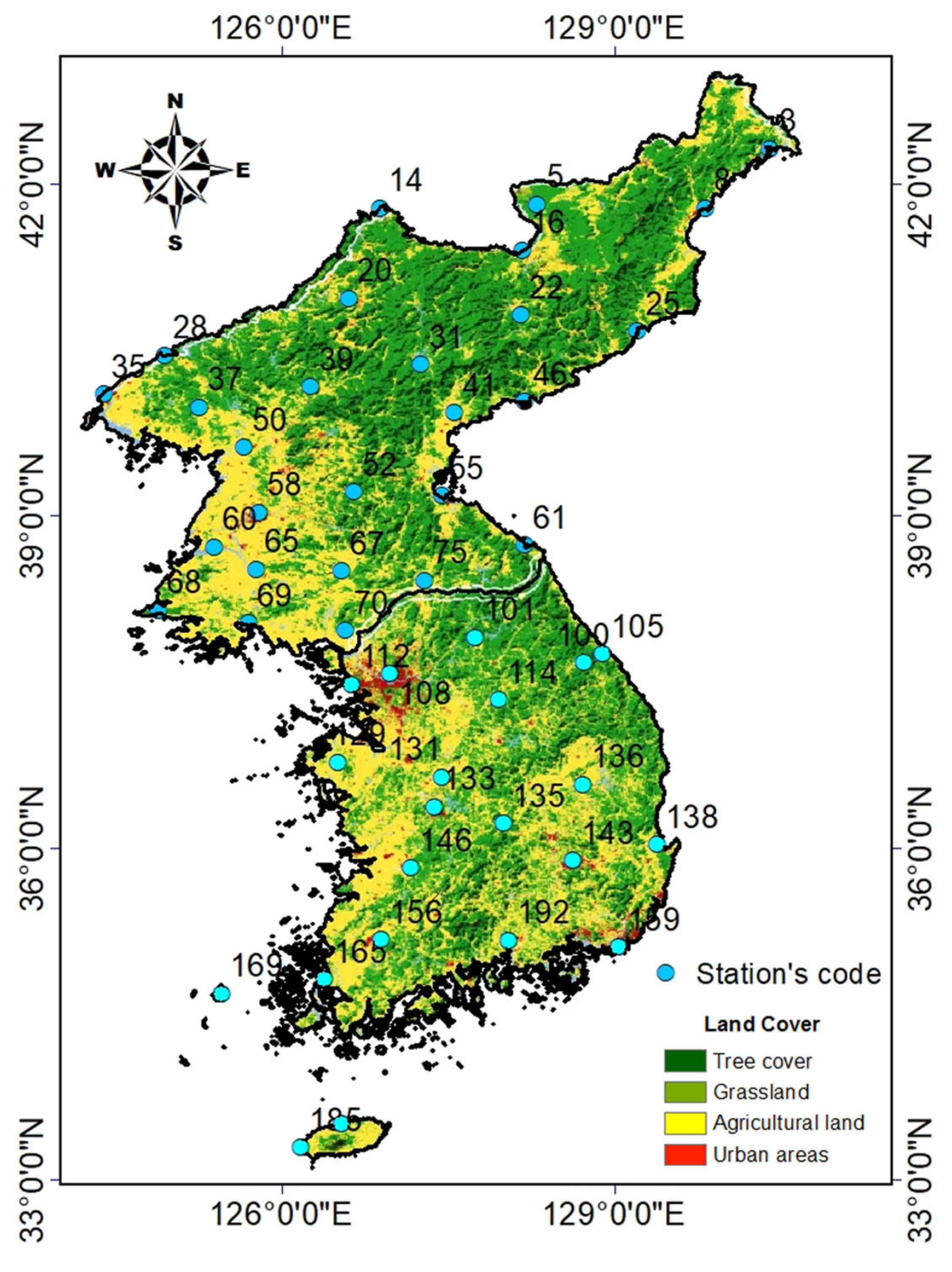
The Korean Peninsula was chosen as the representative region for this study. The Korean Peninsula is a part of East Asia and consists of South Korea (45% of land area) and North Korea (55% of land area). Subtropical monsoons affect the Korean Peninsula, which is nearly 70% mountainous and bounded by three seas: the East Sea, the East China Sea, and the Yellow Sea, resulting in complex atmospheric conditions. The Korean Peninsula can be divided into five distinct regions: a mostly mountainous area in the northern part, the west coast in the western part, the east coast in the eastern part, the south coast in the south, and the plains in the rest of the peninsula. There are four distinct seasons on the Korean Peninsula: spring from March to May, summer from June to August, autumn from September to November, and winter from December to February. The climate significantly varies between seasons due to both continental and oceanic influences, with extremes in summer, impacted by pacific high pressure from the south, and winter, influenced by the cold Siberian air mass [33]. The mean annual precipitation in the Korean Peninsula increases southward, ranging from 1000 mm to 1800 mm. The mean annual temperature ranges from 22.5 °C to 25 °C in summer and from −5 °C to −2.5 °C in winter [34].
This study utilized the Korea Meteorological Administration website to obtain daily climatic data from 21 stations in South Korea and 27 stations in North Korea from 1980 to 2021. Table 1 shows the information on the downloaded meteorological data from the KMA website for both South and North Korea. Only 21 stations in South Korea contained data for observed solar radiation and were selected, and the stations in North Korea had no data for solar radiation. The location and description of the meteorological station is shown in Figure 1 and Table 2.
3. Methods
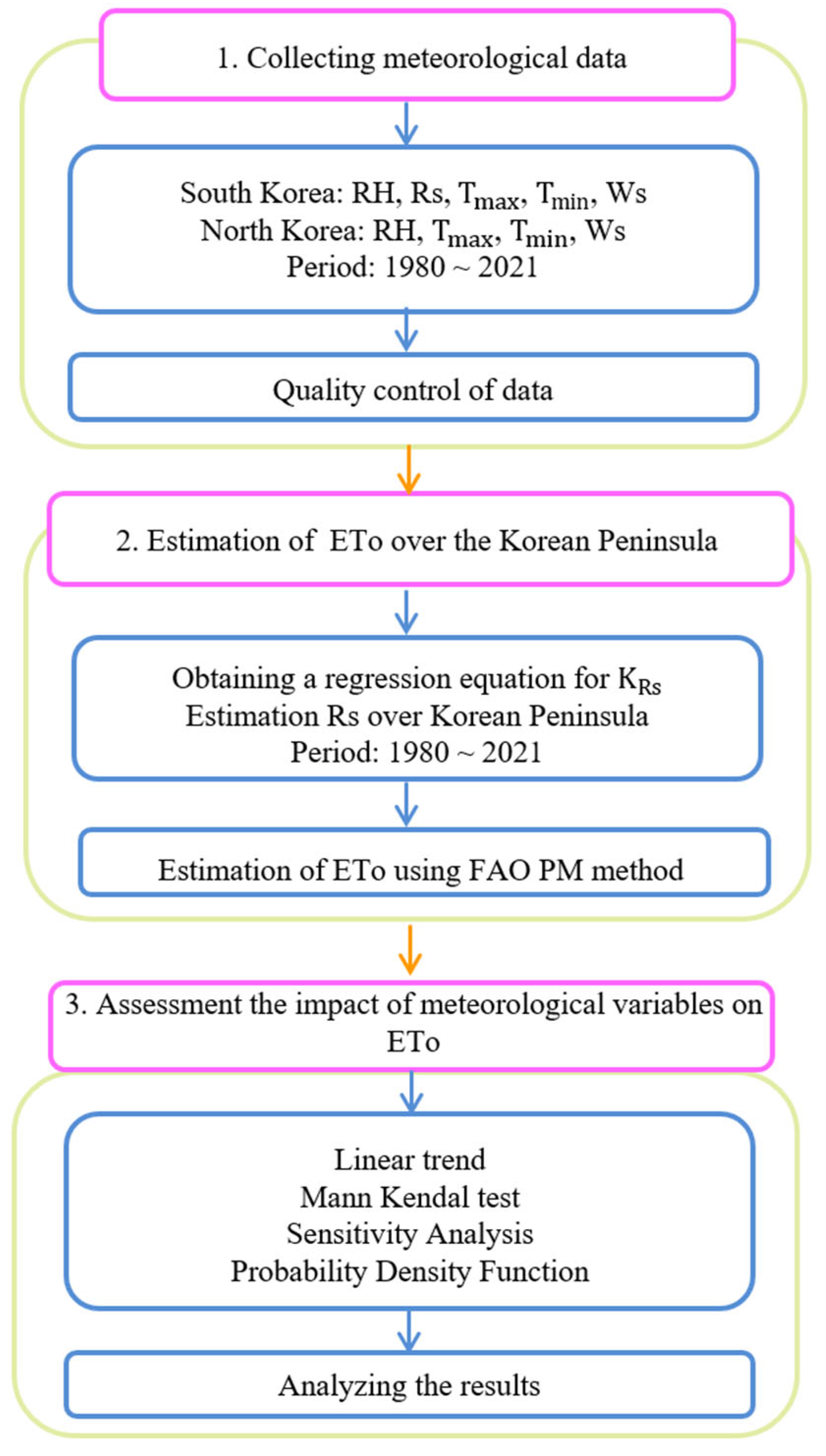
Figure 2 shows the methodology used in this study. The required meteorological data for South Korea and North Korea were extracted for the period 1980 to 2021. In order to estimate Rs over the Korean Peninsula, a regression equation was obtained for , and then Evapotranspiration was calculated over the stations of the Korean Peninsula. The temporal variations of and meteorological variables were analyzed in different geographic conditions to determine how they had changed during the past 42 years in different seasons. Moreover, the Mann-Kendall test was conducted to find significant trends in and meteorological variables. The sensitivity analysis and probability density function of the relative change in were used to determine the most dominate meteorological variables affecting on seasonal and annual scales. In the following sections, the method is explained in detail.
3.1. Estimation of
Whenever data on solar radiation or sunshine hours are unavailable, Allen et al. [12] recommend estimating solar radiation data using the formula developed by Hargreaves and Samani [35]:
where (°C) is the maximum temperature, (°C) is the minimum temperature, represents the extraterrestrial solar radiation (MJ m−2 d−1), and is a coefficient of adjustment, which is calculated using a regression equation. In order to estimate an accurate value of solar radiation, needs to be calibrated for each station in the Statistical Package for the Social Sciences (SPSS) software as an independent variable, and the long-term observations of ( is the mean temperature, and TD is the difference between maximum and minimum temperatures) and EL (elevation) as dependent variables. The results of this analysis were reported in the Coefficient Table of SPSS software to determine the most suitable equation for . In SPSS, the significant value should be compared to 0.05 when testing the hypothesis. If the significant value is greater than 0.05, it means the null hypothesis is accepted. If the significant value is less than 0.05, it shows a rejection of the null hypothesis.
Since there are no data for North Korea, a regional calibrated model for was constructed for South Korea based on the observed data in South Korea. This formula was then used to estimate in both South Korea and North Korea. Using multiple regression analysis, Equation (2) was derived using the mean values over the long term of and EL as the independent variables, and the values of as the dependent variables.
By having the , Equation (1) was used to estimate daily over the Korean Peninsula. It should be noted that was regionally calibrated using observed solar radiation data in South Korea, and therefore, it may be subject to uncertainty in the estimated for stations in North Korea. Table 3 shows the comparison between calculated daily by using observed and estimated daily during 1980–2021 for the stations in South Korea. Based on the results, the root mean square error (RMSE) for all stations was low and the determination coefficient (R2) was high, which determined the good correlations for computed by observed and estimated .
3.2. Estimation of
There are different empirical formulas available for estimations of depending on the availability of meteorological data in the past [36]. When all required data were available, the FAO PM method described by Allen et al. [12] was directly used to estimate daily . The input data required for the FAO PM method were determined using daily maximum air temperature , minimum air temperature , solar radiation , relative humidity , and wind speed . The FAO PM method is expressed in Equation (3):
where is the reference evapotranspiration [mm day−1], is the net radiation at the crop surface [MJ m−2 day−1], G is the soil heat flux density [MJ m−2 day−1], T is the mean daily air temperature at 2 m height [°C], is the wind speed at 2 m height [m s−1], is the saturation vapor pressure [kPa], is the actual vapor pressure [kPa], is the saturation vapor pressure deficit [kPa], Δ is the slope of the vapor pressure curve [kPa °C−1], and is a psychrometric constant [kPa °C−1]. Whenever there are missing data or they cannot be calculated, it is recommended that the user estimates the missing climatic data using one of the procedures described in Chapter 3, by Allen et al. [4]. While there are some alternative methods for calculating that require fewer meteorological parameters, they are less recommended. The data on solar radiation was only available for South Korean stations, so we developed a regression equation to estimate the data for North Korea as explained in the next section.
3.3. The Impact of Meteorological Variables on
In order to identify significant trends and to understand how and meteorological variables have changed over the past 42 years on the Korean Peninsula, seasonal and annual trends of and meteorological variables were analyzed. Sensitivity analysis was used to detect the possible change in caused by variation in meteorological variables. In addition, the probability density function was used to provide the probability density function of change due to the change in meteorological variables. Analysis was completed for both annual and seasonal scales. The standard slope in the linear regression (as defined by B) reflects the percentage of increase or decrease in and meteorological variables in a time series.
3.3.1. Mann-Kendall Test
A Mann-Kendal (MK) test is a nonparametric statistical test which is recommended to determine if the trend in the dataset is significant over time (increasing or decreasing). The MK test was used in this study to assess the significance of seasonal and annual trends of and meteorological variables in different geographic conditions. This method is commonly used to identify trends in meteorological variables, and can be found in [37] and [1]. The statistics of the Mann-Kendall test are determined as follows:
where S denotes the test statistics, n indicates the length of the data set, and indicate the sequential values, is the number of ties of extent i, m is the number of tied groups, and Z is the standardized Mann-Kendall statistic. A pre-whitening method was also used to eliminate serial correlations in the time series of and its climate variables [38,39].
3.3.2. Sensitivity Analysis
Sensitivity analysis is widely used to identify the changes in the dependent variable () caused by the change in an independent meteorological variable (e.g., [40,41,42,43]). For compound models (such as the FAO PM model), it is difficult to compare sensitivity based on partial derivatives, since meteorological variables have different dimensions [23]. As a result, a dimensionless index is derived from the partial derivative [44]:
where represents the sensitivity coefficient, is the actual change of meteorological variable , and is the actual change in induced by . The sign of determines how responds to codirectional changes in input parameters. The sign of determines how would codirectionally react to the input parameter change. For example, a positive of a meteorological parameter indicates that will increase as the variable increases. In addition, the absolute value of indicates the magnitude of response to that meteorological variable [42,43,44,45].
In this study, sensitivity analysis of was calculated for meteorological variables (i.e.,,, , , and ) for ±5%, ±10%, ±15%, and ±20% for each of the variables, while keeping other meteorological variables constant. In order to calculate the mean seasonal and annual , daily values were averaged for different geographical conditions on seasonal and annual scales.
The average values were calculated using geospatial interpolation instead of simple averaging. Spatial averaging involves different methods, including inverse distance weighting (IDW) and kriging. It is used for spatial averaging along surfaces. The IDW combines a set of sample points linearly weighted. Weight is determined by inverse distance. A kriging method, however, generates an estimated surface from a scattering of points by computing kriging weights. A kriging weight value was obtained for each station in this study using the geographical information system (GIS) Spatial Analyst. In this study, the kriging method [46] was used to interpolate the mean seasonal and annual sensitivity coefficients of all stations. This method is widely used by researchers for interpolating data to have the mean value or spatial distribution of a station [47,48,49]. A higher mean value of the sensitivity coefficient indicates that is more sensitive to changes in meteorological variables.
3.3.3. Probability Density Function
The kernel distribution produces the probability density function (PDF) by summing the smooth curves for each data value, which creates a smooth, continuous probability density function for the dataset. In fact, in a non-parametric distribution, the density is entirely determined by the data without any strict distributional assumptions [50]. In other words, nonparametric statistical procedures do not estimate parameters regarding the shape or form of the PDF. Kernel distributions provide nonparametric probability density estimates rather than selecting a density with a specific parametric form and estimating its parameters. The density curve is generated by a kernel density estimator, a smoothing function that determines the shape of the PDF, along with a bandwidth value that controls its smoothness. In the present study, Kernel Density Estimation, which is a nonparametric technique for density estimation, was used to provide the probability density function of percent change due to the percent change in meteorological variables. Kernel density estimation for the relative change of from −20% to +20% change in each meteorological variables was constructed using following equation. Given a random with a continuous univariate density f, the kernel density estimator is [51]:
where K is kernel, is the height of the curve at x (percent change of ), x is relative change of meteorological variable from −20% to 20%, K (.) is the standard normal density, and h is the bandwidth of the density curve.
4. Results
4.1. Mean Seasonal and Annual and Meteorological Variables
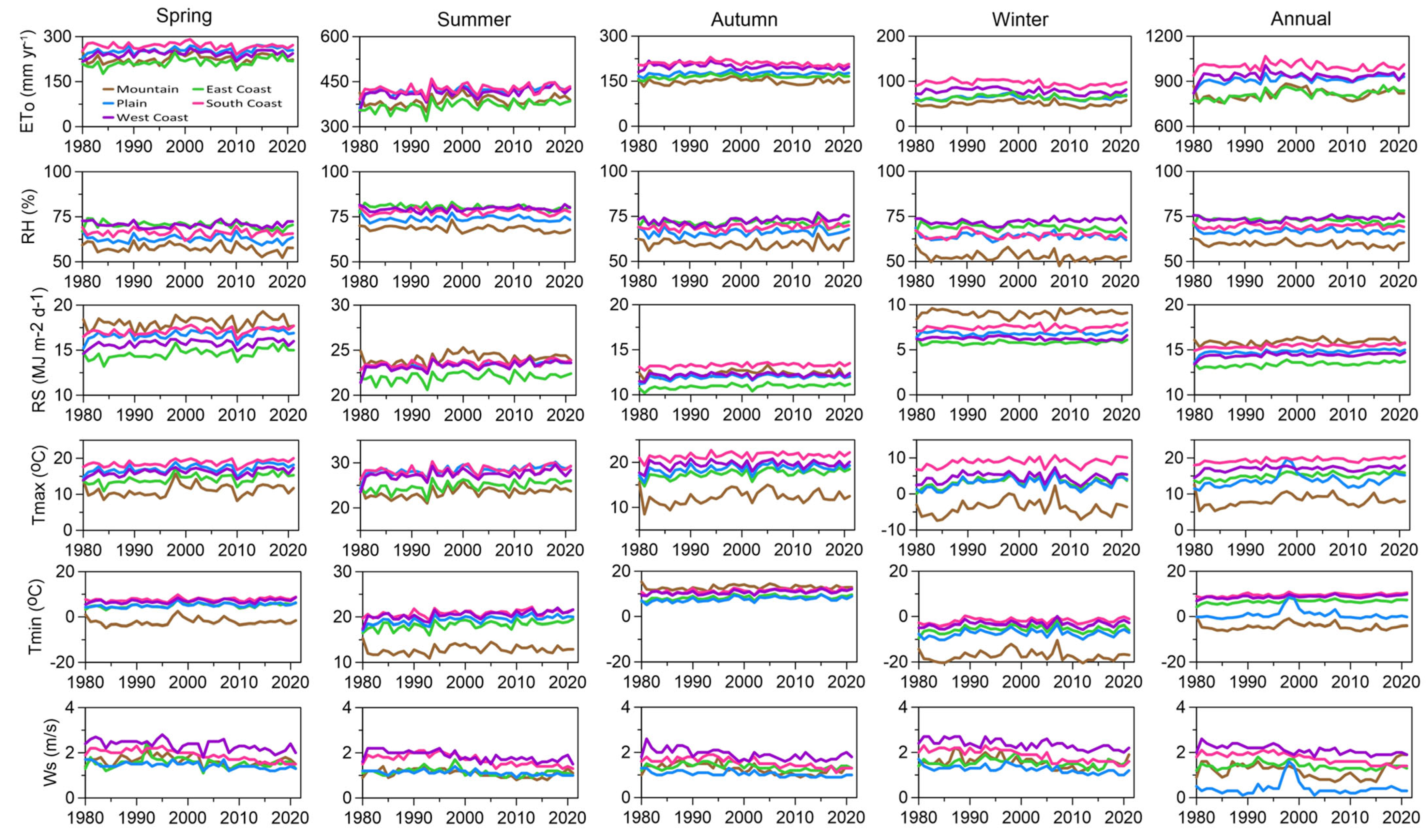
Temporal variation in and meteorological variables over the different regions (i.e., mountainous area, plain area, west coast, east coast, and south coast) are plotted in Figure 3, and the statistical results are reported in Table 4. The trend in the slope of the mean annual is highest in the east coast compared to the other regions. There is an increasing trend in the linear trend of mean annual over the Korean Peninsula from 1980 to 2021 at a rate of in the east coast, in the plain area, and in the mountainous area; however, the south coast revealed a slightly decreasing trend for annual . By neglecting the slightly increasing trend for in the winter season in the east coast, it could be concluded that the linear trend on the seasonal scale increases in all seasons except winter, which exhibits a decreasing trend range from in the south coast to in the west coast. Moreover, summer has the greatest seasonal rate of change in for all regions. Increasing trends in in South Korea are consistent with the results of a study conducted by Aydin et al. [52], which defined the increasing trend for pan evaporation and potential evapotranspiration in South Korea from 1980 to 2009.
According to Table 4, the highest mean annual occurred in the south coast (1000.39 mm/yr), west coast (934.47 mm/yr), and then the plain area (912.28 mm/yr); however, the mean annual ET was lowest along the east coast (813.50 mm/yr) and in mountainous areas (912.28 mm/yr). In all regions, summer had the highest seasonal value, and winter had the lowest.
There was a higher mean value of RH in coastal regions, particularly on the west and east coasts, while the lowest relative humidity was found in mountainous areas. In the mountainous area and on the east coast, the linear trend showed a decreasing trend for seasonal and annual relative humidity. Water availability decreased in the northern and eastern parts of this area, while it increased in other areas of the Korean Peninsula. According to these results, the RH trend over the Korean Peninsula displayed conflicting behavior.
The results of the linear trend of showed increasing trends on seasonal and annual scales over the Korean Peninsula (0.01–0.02 MJm−2d−1yr−1). The maximum increasing trends of occurred in summer and then in the spring over the Korean Peninsula, with the higher value in the mountainous area. The increasing trend in was reported by Russak [53], which concluded that the increase in trend could be a result of decreasing trends in cloudiness and aerosol thickness.
Moreover, the time series of and exhibited an increasing trend, with a higher slope for than that for in the plain area (autumn and winter) and west coast (during all seasons except spring). Based on this pattern, TD (amount of difference between a maximum and a minimum temperature) declined, suggesting that global warming has become more influential in this region, due to increased urbanization and higher aerosol concentrations in this area. However, in other areas, a higher slope for than caused the increasing trend for TD, and therefore, the decreasing trend for . Because TD is related to [54] and cloud effects, accordingly, TD decreases as cloudiness increases, and is correlated with a deficit in vapor pressure [55]. Therefore, decreasing trends in TD caused an increasing trend in in the west coast and plain area, while the increasing trend in TD caused a decreasing trend in , especially in the mountainous area.
According to the results of the trend analysis of wind speed over the Korean Peninsula, showed almost constant downward trends on both an annual and seasonal basis. showed the same slope of decreasing trend (−0.01 m s−1), with a higher decreasing rate in the south coast (−0.02 m s−1) during the spring and winter seasons.
Overall, the trend in reflects the combined impact of all meteorological variables. Generally, the highest has been recorded in the southern part of the Korean Peninsula. The rising trend on Korea’s peninsula over the past 42 years may have been primarily caused by significant increases in and decreases in RH. Furthermore, the outweighing increases in climate parameters in the southern part of the peninsula result in a higher increase in in comparison to the northern part.
4.2. Significant Trends of and Meteorological Variables on Seasonal and Annual Scale
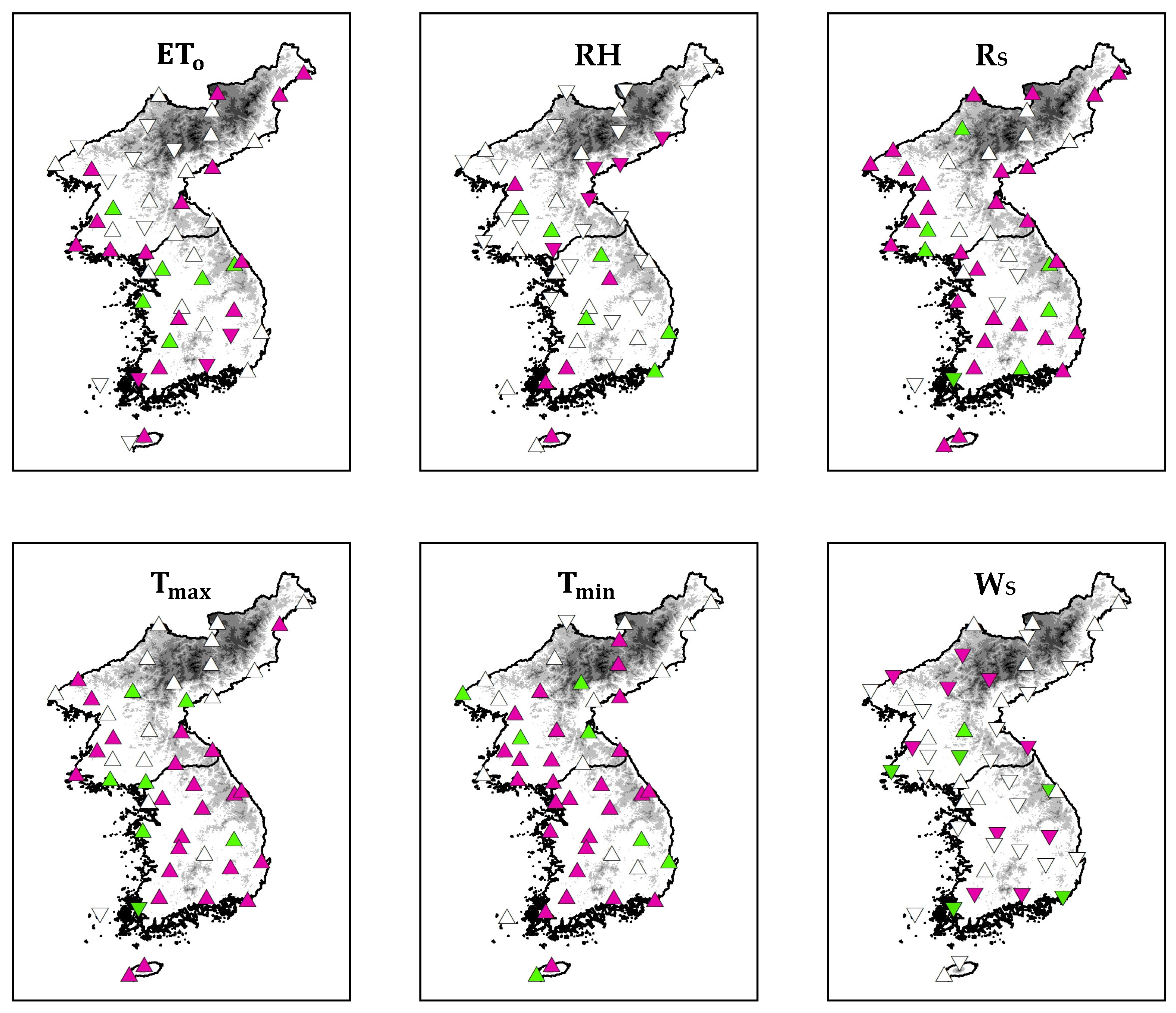
Mann-Kendall tests were conducted on pre-whitened time series in order to assess how trends and meteorological variables have changed over the past 42 years. Figure 4 depicts the spatial distribution of trends at stations on an annual scale. The results for the seasonal and annual scales are also shown in Table 5, which shows how many stations in each region show significant increases, significant decreases, and non-significant trends.
showed significant increases mainly along the east coast, plain area, and south coast; however, the mountainous region did not show any significant changes. The significant increasing trends on the east coast were mainly driven by a significant decrease in . Furthermore, the significant increasing trends in the plain area and south coast occurred due to the most striking trends in , , and . Moreover, most stations in the south coast of the peninsula indicated a significant decreasing trend, which mainly occurred because of significant decreasing trends in , , and .
4.3. Sensitivity Analysis of Meteorological Variables to Change over the Korean Peninsula
The daily sensitivity coefficients of with respect to the key meteorological variables was calculated for all stations, and then the station value sensitivity coefficient was obtained for all meteorological variables on both a seasonal and annual basis. The sensitivity coefficient can be used to quantitatively analyze changes in by changing one variable, while other variables remain constant. Percentage changes in relative to changes in meteorological variables for each season and annual were obtained.
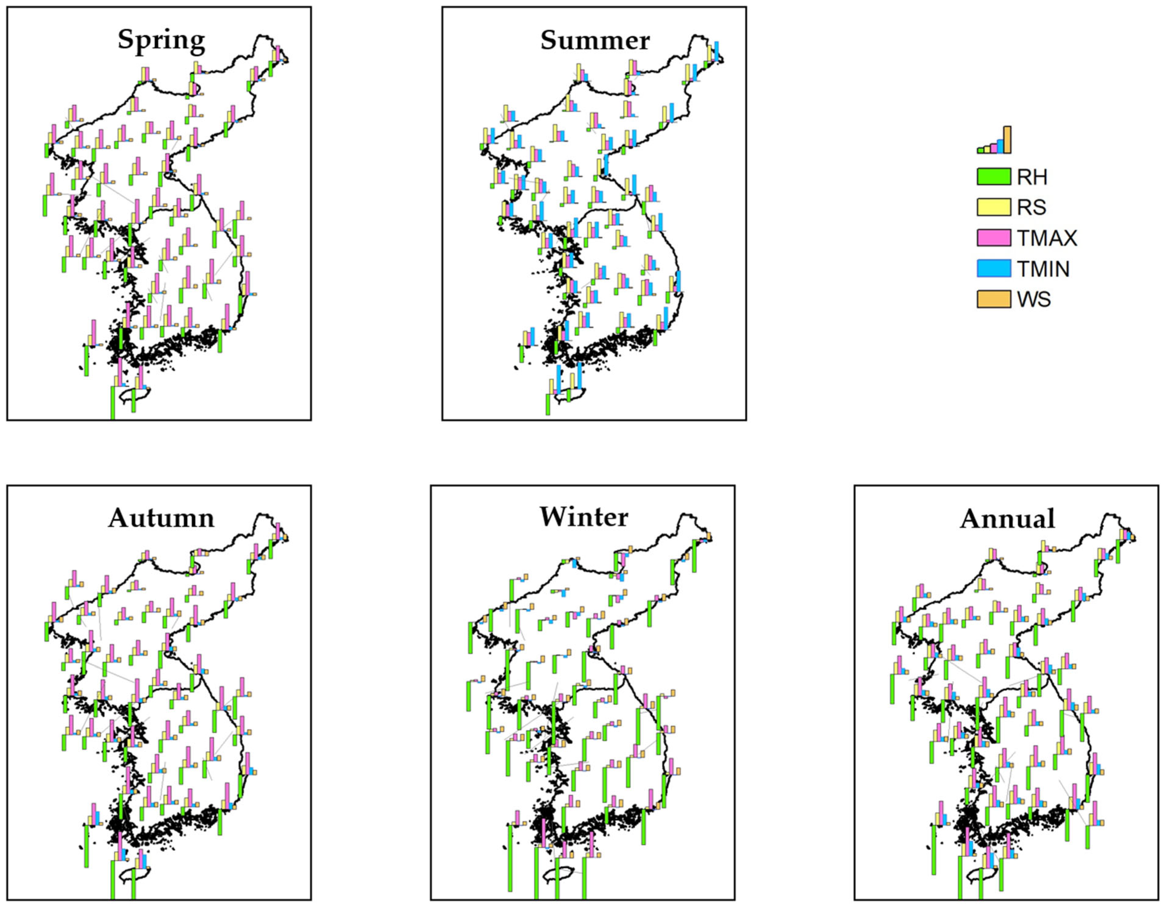
The bar charts in Figure 5 show the seasonal and annual sensitivity coefficients of meteorological variables over the Korean Peninsula, and the statistics are reported in Table 6. The spatial distribution of sensitivity coefficients indicated that the sensitive parameters are different in each season. According to the spatial distribution of the sensitivity coefficient, each season has different sensitive parameters. In spring and autumn, responds almost in the same way to changes in meteorological variables, but, in summer and winter, this response is significantly different.
The most sensitive parameters to change in spring and autumn are and ; however, in summer, , , and have the greatest impact on . In winter, is the key parameters to affect and the northern part of the Korean Peninsula is more sensitive to change in than the southern part. However, some stations in the mountainous area are more sensitive to because the northern part of the peninsula is more impacted by Siberia’s cold weather in winter.
In general, the following results were obtained by sensitivity analysis: (i) , followed by , are the most sensitive parameters in spring for all regions, with very high sensitivity in the south coast and west coast. (ii) In summer, the coastal areas have high sensitivity to the change in (especially the south coast, with SC= 1.12); however, the mountainous and plain areas are the most sensitive to and . (iii) In autumn, is the main parameter that influences , followed by , with very high sensitivity in the south coast and the west coast. However, in other regions, the increase in followed by a decrease in is the key change that affects in autumn. (iv) Winter shows the highest sensitivity among the seasons for all regions. In fact, the winter season is the driest season in the Korean Peninsula and is very sensitive to the change in , with high sensitivity in the coastal regions. (v) On an annual scale, the average value of sensitivity analysis coefficients can be ranked as in the mountainous and plain areas, and in the coastal areas. Overall, analysis showed that the two major components to change are and over the Korean Peninsula.
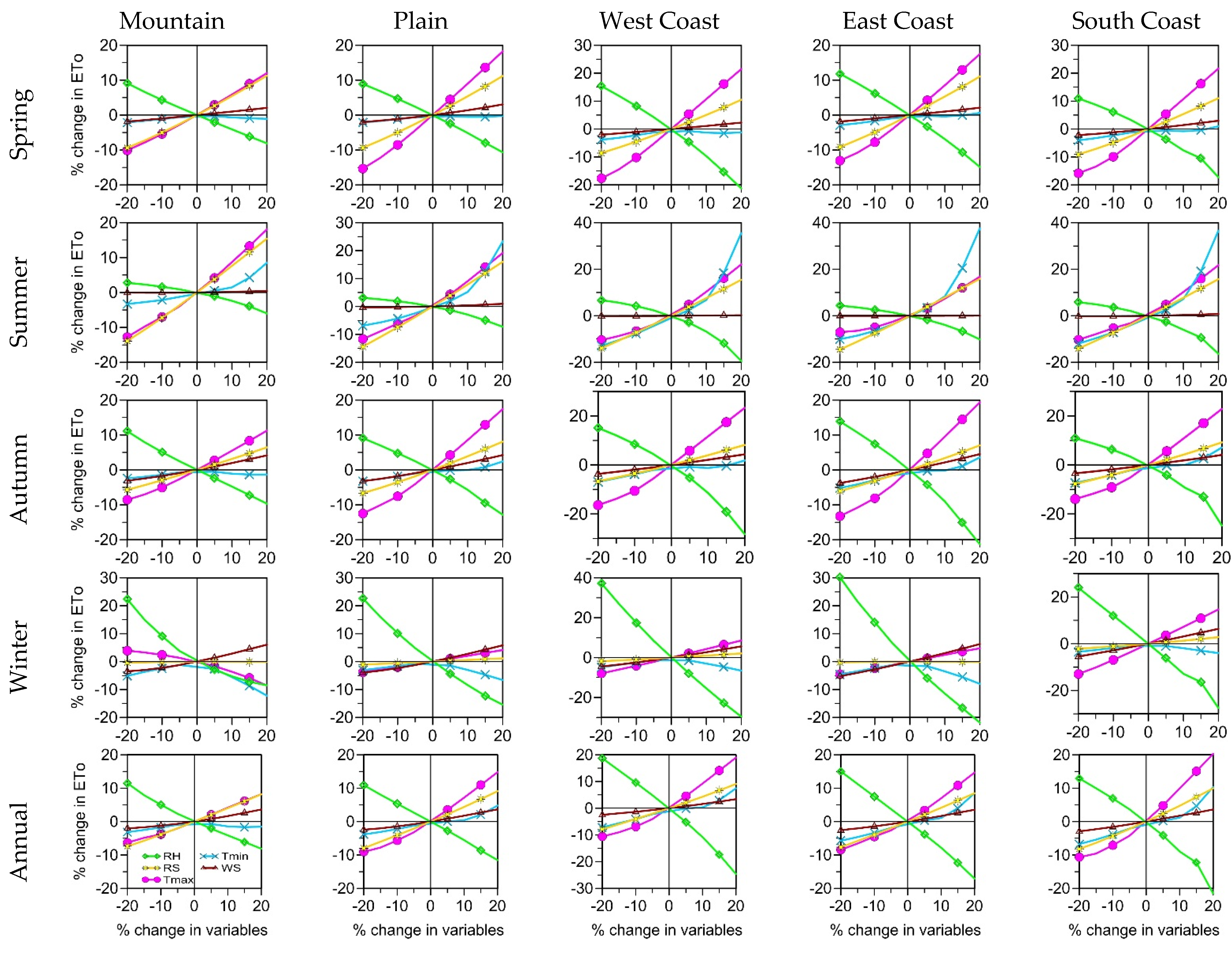
Figure 6 illustrates the amount of change in by changing the meteorological variables from −20% to +20 with a 5% interval. Based on the relative change in , different geographical conditions respond differently to changes in meteorological variables, with coastal areas exhibiting higher variability than mountainous and plain areas. Additionally, meteorological variables vary from season to season. In general, RH responds most strongly to changes in except in the summer season. A high-pressure system over the western North Pacific and the Indian summer monsoon contribute to high relative humidity during summer monsoons. As a result, is not sensitive to changes in RH in summer; however, other seasons, especially winter, which is the driest season on the Korean Peninsula, are highly sensitive to changes in RH.
4.4. Probability Density Function of Meteorological Variables to Change over the Korean Peninsula
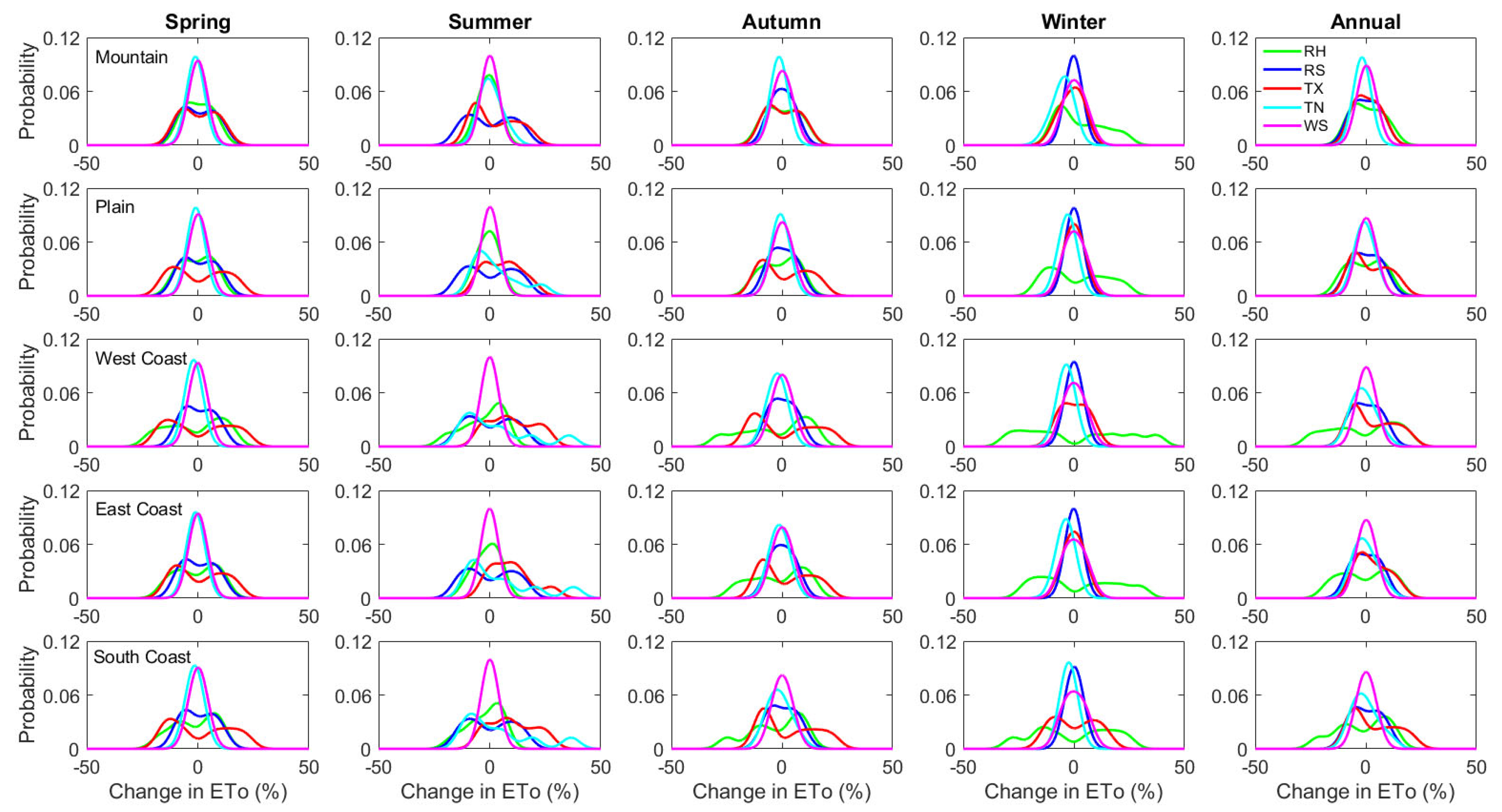
The probability density function (PDF) of percent change of due to changes in meteorological parameters on seasonal and annual scales in different regions was obtained using a Kernel Density Estimator and is illustrated in Figure 7. The wider shape of the distribution from the normal distribution indicated more variability of meteorological parameters to change . The relative change in caused by percent change of each meteorological variables from −20% to +20% with intervals of 5% was shown as the probability density function during the seasonal and annual scales (Figure 7), which demonstrated the impact of meteorological variables varied during the seasons and throughout regions. In fact, changes in meteorological variables caused changes in the mean, variance, and shape of the distribution, which were different in each season and each geographic condition. According to the results, responded differently to changes in meteorological variables based on geographic location. The shape of PDF near the normal distribution shows lower sensitivity, while dispersion from the normal distribution (mean) indicates the higher sensitivity of by changing meteorological variables. In spring, the shape of the distribution was shifted from a normal distribution for and in spring, especially for the coastal area, indicating higher sensitivity of to change those variables in this season. In summer, , , and , and in autumn, and , are more dispersed from the mean, which shows the higher sensitivity of to change them. However, in winter, is the most sensitive parameter for all geographic conditions (with a higher sensitivity in coastal areas).
5. Discussion
The Korean Peninsula is affected by surrounded seas. The peninsula is also impacted by the Pacific Ocean over the Japanese archipelago. Therefore, the climatic conditions of the peninsula are impacted by both the ocean and the continent, leading to significant seasonal variability, such as monsoons [56]. In fact, the summer season in the Korean Peninsula is warm and wet, which is driven by the ocean, while the winter season is cold and dry, driven by the Siberian cold air mass (continental effect). Temporal variations of the showed that the southern coast recorded the highest mean seasonal and annual values. Similar to the mountainous area, the east coast had the lowest on a seasonal and annual basis. The results showed that meteorological variables have different tendencies to change over the Korean Peninsula.
The results of the study by Nie et al. [57] showed that the sensitivity coefficient and contribution rate of to meteorological factors vary by climatic region in China. Sensitivity coefficients and contribution rates to spatially vary even within the same climatic region. In this study, the slope of the temporal trends indicates a decreasing trend for the south coast and an increasing trend for the east coast. The reason for the decreasing trend in on the south coast is the increasing trend in RH, which is affected by TD. In fact, on the south coast, the rising trend of is higher than , leading to a decreasing trend in TD, and therefore, an upward trend in RH. The increasing trend in due to a deficiency in RH was reported in Iran [9] and China [26,29]. In mountainous areas, affected by continental influence in the northern part of the Korean Peninsula, the mean is the lowest. While in coastal areas, particularly on the east coast and south coast, RH is the highest. in spring and summer has the highest value in the mountainous area in the northern Korean Peninsula, while autumn has the maximum value in the south coast and the minimum value in the east coast. The mean annual and seasonal temperature increases from north to south. and have the main influence on changing in the North China plain [28]. Furthermore, the mean and are highest in the south coast and decline toward the west coast and east coast. The higher temperature in the southern part of the Korean Peninsula is related to the Tsushima Warm Current. However, the mountainous area has the minimum value of maximum and minimum temperature, since this area is affected by the North Korea Cold Current. The sensitivity of to change was also reported in a semi-arid region in India [25]. Moreover, the showed decreasing trends among all seasons and regions. Significant decreases in wind speed have recently been reported in different countries. Land use changes and increased surface roughness near meteorological stations have been attributed to the decrease in trend. Similar results were reported in [28,30]. The weakening trend in may occur due to temperature increases due to global change. According to the findings of Xiaomei et al. [58], the increasing trends in and cause decreases in , and it may be concluded that changes in temperature indirectly influence other meteorological variables.
This study was based on a 42-year historical dataset, and the impact of climate change was not taken into consideration. Therefore, we suggest following the same methodology by using global climate models to examine the impact of the main meteorological variables on under different geographical conditions. Furthermore, we recommend assessing the risk and vulnerability by taking into account the change in , and implementing the necessary strategy and deployment plan to ensure a sustainable water supply. Furthermore, we recommend conducting a similar study to compare the impact of meteorological variables to change water budgets, including evapotranspiration, precipitation, and discharge changes in different geographical conditions.
6. Conclusions
In this study, we examined the impacts of meteorological variables on across different geographic conditions on the Korean Peninsula, using a 42-year daily dataset. It was found that seasonal and regional changes were influenced differently by different meteorological variables. In the summer, coastal areas showed higher sensitivity to the increase in . In contrast, autumn and spring were the most sensitive to the increase in . This indicated that, for analyzing the impact of the meteorological variables, is not the appropriate variable and the influence of both and should be considered. In all regions, winter was the most sensitive to changes in , particularly on the east and west coasts. Among all Korean Peninsula regions, winter and summer were the most sensitive seasons. The magnitudes of sensitive parameters during each season varied depending on location, according to the spatial distribution of those parameters. As a result of the study, it can be determined that different seasons have different responses to changes in maximum and minimum temperatures, and, for a better understanding of the change of to changes in temperature, both the maximum and minimum temperatures should be considered instead of . Moreover, comparison between the sensitive coefficients of the seasonal and annual scales showed that it is not enough to only consider the impact of sensitive parameters for the annual scale. Although it revealed the key sensitive parameters in each region, different parameters have different responses in each season and in each region.
Author Contributions
Conceptualization, M.G.-A.; Data curation M.G.-A.; Formal analysis, M.G.-A.; Funding acquisition, S.-I.L.; Methodology, M.G.-A.; Project administration, S.-I.L.; Supervision, S.-I.L.; Visualization, M.G.-A.; Writing—original draft, M.G.-A.; Writing—review and editing, M.G.-A. and S.-I.L. All authors have read and agreed to the published version of the manuscript.
Funding
This work was supported by the National Research Foundation of Korea (NRF) grant by the Korea government (2021R1A2C2011193).
Institutional Review Board Statement
Not applicable.
Informed Consent Statement
Not applicable.
Data Availability Statement
Not applicable.
Conflicts of Interest
The authors declare no conflict of interest.
References
- Gocic, M.; Trajkovic, S. Analysis of trends in reference evapotranspiration data in a humid agricultural water management climate. Hydrol. Sci. J. 2014, 59, 65–180. [Google Scholar] [CrossRef]
- Valipour, M.; Bateni, S.M.; Gholami Sefidkouhi, M.A.; Raeini-Sarjaz, M.; Singh, V.P. Complexity of Forces Driving Trend of Reference Evapotranspiration and Signals of Climate Change. Atmosphere 2020, 11, 1081. [Google Scholar] [CrossRef]
- Luo, Y.; Gao, P.; Mu, X. Influence of Meteorological Factors on the Potential Evapotranspiration in Yanhe River Basin, China. Water 2021, 13, 1222. [Google Scholar] [CrossRef]
- McNally, A.; Arsenault, K.; Kumar, S.; Shukla, S.; Peterson, P.; Wang, S.; Funk, C.; Peters-Lidard, C.D.; Verdin, J.P. A land data assimilation system for sub-Saharan Africa food and water security applications. Sci. Data 2017, 4, 170012. [Google Scholar] [CrossRef] [Green Version]
- Muhammad Adnan, R.; Chen, Z.; Yuan, X.; Kisi, O.; El-Shafie, A.; Kuriqi, A.; Ikram, M. Reference Evapotranspiration Modeling Using New Heuristic Methods. Entropy 2020, 22, 547. [Google Scholar] [CrossRef]
- Zhang, X.; Kang, S.; Zhang, L.; Liu, J. Spatial variation of climatology monthly crop reference evapotranspiration and sensitivity coefficients in Shiyang river basin of northwest China. Agric. Water Manag. 2010, 97, 1506–1516. [Google Scholar] [CrossRef]
- Sahoo, B.; Walling, I.; Deka, B.C.; Bhatt, B.P. Standardization of Reference Evapotranspiration Models for a Subhumid Valley Rangeland in the Eastern Himalayas. J. Irrig. Drain. Eng. 2012, 138, 880–896. [Google Scholar] [CrossRef]
- Srivastava, A.; Sahoo, B.; Raghuwanshi, N.S.; Singh, R. Evaluation of Variable-Infiltration Capacity Model and MODIS-Terra Satellite-Derived Grid-Scale Evapotranspiration Estimates in a River Basin with Tropical Monsoon-Type Climatology. J. Irrig. Drain. Eng. 2017, 143, 04017028. [Google Scholar] [CrossRef] [Green Version]
- Bakhtiari, B.; Liaghat, A.M. Seasonal Sensitivity Analysis for Climatic Variables of ASCE Penman-Monteith Model in a Semi-Arid Climate. J. Agric. Sci. Technol. 2011, 13, 1135–1145. [Google Scholar]
- Pandey, P.K.; Dabral, P.P.; Pandey, V. Evaluation of reference evapotranspiration methods for the northeastern region of India. Int. Soil Water Conserv. Res. 2016, 4, 52–63. [Google Scholar] [CrossRef] [Green Version]
- Pandey, P.K.; Nyori, T.; Pandey, V. Estimation of reference evapotranspiration using data driven techniques under limited data conditions. Model. Earth Syst. Environ. 2017, 3, 1449–1461. [Google Scholar] [CrossRef]
- Allen, R.G.; Pereira, L.S.; Raes, D.; Smith, M. Crop Evapotranspiration—Guidelines for Computing Crop Water Requirements-FAO Irrigation and Drainage Paper 56; Food and Agriculture Organization of the United Nations: Rome, Italy, 1998. [Google Scholar]
- Vicente-Serranoa, S.M.; Azorin-Molinaa, C.; Sanchez-Lorenzoa, A.; Revuelto, J.; López-Morenoa, J.I.; González-Hidalgoc, J.C.; Moran-Tejedaa, E.; Espejod, F. Reference evapotranspiration variability and trends in Spain, 1961–2011. Glob. Planet. Chang. 2014, 121, 26–40. [Google Scholar] [CrossRef] [Green Version]
- Nouri, M.; Homaee, M.; Bannayan, M. Spatiotemporal reference evapotranspiration changes in humid and semi-arid regions of Iran: Past trends and future projections. Theor. Appl. Climatol. 2018, 133, 361–375. [Google Scholar] [CrossRef]
- Nouri, M.; Homaee, M.; Bannayan, M. Quantitative trend, sensitivity and contribution analyses of reference evapotranspiration in some arid environments under climate change. Water Resour. Manag. 2017, 31, 2207–2224. [Google Scholar] [CrossRef]
- Yan, X.; Mohammadian, A.; Ao, R.; Liu, J.; Chen, X. Spatiotemporal Variations in Reference Evapotranspiration and Its Contributing Climatic Variables at Various Spatial Scales across China for 1984–2019. Water 2022, 14, 2502. [Google Scholar] [CrossRef]
- Dinpashoh, Y.; Babamiri, O. Trends in reference crop evapotranspiration in Urmia Lake basin. Arab. J. Geosci. 2020, 13, 372. [Google Scholar] [CrossRef]
- Ndiaye, P.M.; Bodian, A.; Diop, L.; Deme, A.; Dezetter, A.; Djaman, K.; Ogilvie, A. Trend and Sensitivity Analysis of Reference Evapotranspiration in the Senegal River Basin Using NASA Meteorological Data. Water 2020, 12, 1957. [Google Scholar] [CrossRef]
- Da Silva, V.D.P.R. On climate variability in northeast of Brazil. J. Arid Environ. 2004, 58, 575–596. [Google Scholar] [CrossRef]
- Darshana; Pandey, A.; Pandey, R.P. Analysing trends in reference evapotranspiration and weather variables in the Tons River Basin in Central India. Stoch. Environ. Res. Risk Assess. 2013, 27, 1407–1421. [Google Scholar] [CrossRef]
- Obada, E.; Alamou, E.A.; Chabi, A.; Zandagba, J.; Afouda, A. Trends and Changes in Recent and Future Penman-Monteith Potential Evapotranspiration in Benin (West Africa). Hydrology 2017, 4, 38. [Google Scholar] [CrossRef] [Green Version]
- Sharifi, A.; Dinpashoh, Y. Sensitivity Analysis of the Penman-Monteith reference Crop Evapotranspiration to Climatic Variables in Iran. Water Res. Manag. 2014, 28, 5465–5476. [Google Scholar] [CrossRef]
- Seong, C.; Sridhar, V.; Billah, M.M. Implications of potential evapotranspiration methods for streamflow estimations under changing climatic conditions. Int. J. Climatol. 2018, 38, 896–914. [Google Scholar] [CrossRef]
- Irmak, S.; Payero, J.O.; Martin, D.L.; Irmak, A.; Howell, T.A. Sensitivity analyses and sensitivity coefficients of standardized daily ASCE-Penman-Monteith equation. J. Irrig. Drain. Eng. 2006, 132, 564–578. [Google Scholar] [CrossRef]
- Goyal, R.K. Sensitivity of evapotranspiration to global warming: A case study of arid zone of Rajasthan (India). Agric. Water Manag. 2004, 69, 1–11. [Google Scholar] [CrossRef]
- Liqiao, L.; Li, L.; Zhang, L.; Li, J.; Li, B. Sensitivity of Penman-Monteith reference crop evapotranspiration in Tao’er River Basin of northeastern China. Chin. Geogr. Sci. 2008, 18, 340–347. [Google Scholar] [CrossRef]
- Estévez, J.; Gavilán, P.; Berengena, J. Sensitivity analysis of a Penman–Monteith type equation to estimate reference evapotranspiration in southern Spain. Hydrol. Process. 2009, 23, 3342–3353. [Google Scholar] [CrossRef]
- Song, Z.; Zhang, H.; Snyder, R.; Anderson, F.; Chen, F. Distribution and trends in reference evapotranspiration in the North China Plain. J. Irrig. Drain. Eng. 2010, 136, 240–247. [Google Scholar] [CrossRef]
- Yang, Z.; Liu, Q.; Cui, B. Spatial distribution and temporal variation of reference evapotranspiration during 1961–2006 in the Yellow River Basin, China. Hydrol. Sci. J. 2011, 56, 1015–1026. [Google Scholar] [CrossRef] [Green Version]
- Porter, D.; Gowda, P.; Marek, T.; Howell, T.; Moorhead, T.J.; Irmak, S. Sensitivity of grass-and alfalfa-reference evapotranspiration to weather station sensor accuracy. Appl. Eng. Agric. 2012, 28, 543–549. [Google Scholar] [CrossRef]
- Hou, L.G.; Zou, S.B.; Xiao, H.L.; Yang, Y.G. Sensitivity of the reference evapotranspiration to key climatic variables during the growing season in the Ejina oasis northwest China. SpringerPlus 2013, 2 (Suppl. 1), S4. [Google Scholar] [CrossRef] [Green Version]
- Liu, Y.; Tang, G.; Wu, L.; Wu, Y.; Yang, M. Variations in reference evapotranspiration and associated driving forces in the Pearl River Delta of China during 1960–2016. J. Meteorol. Soc. Jpn. 2019, 97, 467–479. [Google Scholar] [CrossRef]
- Hwang, J.H.; Van, S.P.; Choi, B.-J.; Chang, Y.S.; Kim, Y.H. The physical processes in the Yellow Sea. Ocean Coast. Manag. 2014, 102, 449–457. [Google Scholar] [CrossRef]
- Teng, S.K.; Yu, H.; Tang, Y.; Tong, L.; Choi, C.I.; Kang, D.; Liu, H.; Chun, Y.; Juliano, R.O.; Rautalahti-Miettinen, E.; et al. Yellow Sea; GIWA Regional Assessment 34; University of Kalmar: Kalmar, Sweden, 2005. [Google Scholar]
- Hargreaves, G.H.; Samani, Z. Estimating Potential Evapotranspiration. J. Irrig. Drain. Div. 1982, 108, 225–230. [Google Scholar] [CrossRef]
- Xu, J.; Haginoya, S.; Saito, K.; Motoya, K. Surface heat balance and pan evaporation trends in eastern Asia in the period 1971–2000. Hydrol. Process. 2005, 19, 2161–2186. [Google Scholar] [CrossRef]
- Hirsch, R.M.; Slack, J.R.; Smith, R.A. Techniques of trend analysis for monthly water quality. Water Resour. Res. 1982, 18, 107–121. [Google Scholar] [CrossRef] [Green Version]
- Von Storch, H.; Navarra, A. Analysis of Climate Variability-Applications of Statistical Techniques; Springer: Berlin/Heidelberg, Germany, 1999. [Google Scholar]
- Jhajharia, D.; Dinpashoh, Y.; Kahya, E.; Singh, V.P.; Fakheri-Fard, A. Trends in reference evapotranspiration in the humid region of northeast India. Hydrol. Process. 2012, 26, 421–435. [Google Scholar] [CrossRef]
- Coleman, G.; DeCoursey, D.G. Sensitivity and model variance analysis applied to some evaporation and evapotranspiration models. Water Resour. Res. 1976, 12, 873–879. [Google Scholar] [CrossRef]
- Hupet, F.; Vanclooster, M. Effect of the sampling frequency of meteorological variables on the estimation of the reference evapotranspiration. J. Hydrol. 2001, 243, 192–204. [Google Scholar] [CrossRef]
- Yin, Y.; Wu, S.; Chen, G.; Dai, E. Contribution analyses of potential evapotranspiration changes in China since the 1960s. Theor. Appl. Climatol. 2010, 101, 19–28. [Google Scholar] [CrossRef]
- Patle, G.T.; Singh, D.K. Sensitivity of annual and seasonal reference crop evapotranspiration to principal climatic variables. J. Earth Syst. Sci. 2015, 124, 819–828. [Google Scholar] [CrossRef] [Green Version]
- McCuen, R.H. A sensitivity and error analysis CF procedures used for estimating evaporation. J. Am. Water Resour. Assoc. 1974, 10, 486–497. [Google Scholar] [CrossRef]
- Gong, L.; Xu, C.Y.; Chen, D.; Halldin, S.; Chen, Y.D. Sensitivity of the Penman–Monteith reference evapotranspiration to key climatic variables in the Changjiang (Yangtze River) basin. J. Hydrol. 2006, 329, 620–629. [Google Scholar] [CrossRef]
- Journel, A.G.; Huijbregts, C.J. Mining Geostatistics; Academic Press: New York, NY, USA, 1978. [Google Scholar]
- Oliver, M.A. Kriging: A Method of Interpolation for Geographical Information Systems. Int. J. Geogr. Inf. 1990, 4, 313–332. [Google Scholar] [CrossRef]
- Xu, C.Y.; Gong, L.; Jiang, T.; Chend, D.; Singh, V.P. Analysis of spatial distribution and temporal trend of reference evapotranspiration and pan evaporation in Changjiang (Yangtze River) catchment. J. Hydrol. 2006, 327, 81–93. [Google Scholar] [CrossRef]
- Liu, Q.; Yang, Z.; Cui, B.; Sun, T. The temporal trends of reference evapotranspiration and its sensitivity to key meteorological variables in the Yellow River Basin, China. Hydrol. Process. 2010, 24, 2171–2181. [Google Scholar] [CrossRef]
- Murphy, K. Machine Learning: A Probabilistic Perspective; MIT Press: Cambridge, MA, USA, 2012; p. 16. [Google Scholar]
- Wand, M.P.; Jones, M.C. Kernel Smoothing, Monographs on Statistics and Applied Probability; Chapman & Hall: Boca Raton, FL, USA, 1995. [Google Scholar]
- Aydin, M.; Jung, Y.S.; Yang, J.E.; Kim, S.J.; Kim, K.D. Sensitivity of soil evaporation and reference evapotranspiration to climatic variables in South Korea. Turk. J. Agric. For. 2015, 39, 652–662. [Google Scholar] [CrossRef]
- Russak, V. Changes in solar radiation and their influence on temperature trend in Estonia (1955–2007). J. Geophys. Res. 2009, 114, D00D01. [Google Scholar] [CrossRef]
- Verhoef, A.; Feddes, R.A. Preliminary Review of Revised FAO Radiation and Temperature Methods; FAO Report 16; Landbouwuniversiteit Wageningen: Wageningen, The Netherlands, 1991; pp. 1–116. [Google Scholar]
- Hargreaves, G.H.; Allen, R.G. History and evaluation of Hargreaves evapotranspiration equation. J. Irrig. Drain. Eng. 2003, 129, 53–63. [Google Scholar] [CrossRef]
- Youn, Y.H. The climate variabilities of air temperature around the Korean Peninsula. Adv. Atmos. Sci. 2005, 22, 575–584. [Google Scholar] [CrossRef]
- Nie, T.; Yuan, R.; Liao, S.; Zhang, Z.; Gong, Z.; Zhao, X.; Chen, P.; Li, T.; Lin, Y.; Du, C.; et al. Characteristics of Potential Evapotranspiration Changes and Its Climatic Causes in Heilongjiang Province from 1960 to 2019. Agriculture 2022, 12, 2017. [Google Scholar] [CrossRef]
- Xiaomei, Y.; Zongxing, L.; Qi, F.; Yuanqing, H.; Wenlin, A.; Wei, Z.; Weihong, C.; Tengfei, Y.; Yamin, W.; Theakstone, W.H. The decreasing wind speed in southwestern China during 1969–2009, and possible causes. Quat. Int. 2012, 263, 71–84. [Google Scholar] [CrossRef]
Figure 1.
Study area.

Figure 2.
Workflow diagram.

Figure 3.
Temporal variation of and meteorological variables on seasonal and annual scales in different geographic conditions (1980–2021).
Figure 3.
Temporal variation of and meteorological variables on seasonal and annual scales in different geographic conditions (1980–2021).

Figure 4.
Spatial distribution of the annual trend of stations for and meteorological variables over the Korean Peninsula (1980–2021). Upward and downward triangles define increasing and decreasing trends, respectively. The pink color indicates 95% confidence level, the green color indicates 90% confidence level, and white color indicates the trend is not significant.

Figure 5.
Spatial distribution of the sensitivity coefficients of to meteorological variables over the Korean Peninsula.
Figure 5.
Spatial distribution of the sensitivity coefficients of to meteorological variables over the Korean Peninsula.

Figure 6.
Relative change in with respect to the percent change of meteorological variables on seasonal and annual scales in different geographic conditions.
Figure 6.
Relative change in with respect to the percent change of meteorological variables on seasonal and annual scales in different geographic conditions.

Figure 7.
Probability density of changes with respect to changes in meteorological variables on seasonal and annual scales in different geographic conditions.
Figure 7.
Probability density of changes with respect to changes in meteorological variables on seasonal and annual scales in different geographic conditions.


Table 1.
The list of the extracted data for this study.
| Weather Observation Data by Country | Variables | Period | Link |
|---|---|---|---|
| South Korea | 1980–2021 | https://data.kma.go.kr/data/grnd/selectAsosRltmList.do?pgmNo=36 (accessed on 20 May 2022). | |
| 1980–2021 | |||
| 1980–2021 | |||
| 1980–2021 | |||
| 1980–2021 | |||
| North Korea | 1980–2021 | https://data.kma.go.kr/data/grnd/selectNkRltmList.do?pgmNo=58 (accessed on 20 May 2022). | |
| 1980–2021 | |||
| 1980–2021 | |||
| 1980–2021 |
Table 2.
Characteristics of the meteorological stations used in this study.
| Station Code | Station Name | Lat. (°) | Lon. (°) | Geography | Ele. (m) | Station Code | Station Name | Lat. (°) | Lon. (°) | Geography | Ele. (m) |
|---|---|---|---|---|---|---|---|---|---|---|---|
| 3 | Seonbong | 42.3 | 130.4 | EC | 3 | 69 | Haeju | 38.0 | 125.7 | WC | 81 |
| 5 | Samjiyeon | 41.8 | 128.3 | M | 1386 | 70 | Gaeseong | 38.0 | 126.6 | P | 70 |
| 8 | Cheongjin | 41.8 | 129.8 | EC | 43 | 75 | Pyeonggang | 38.4 | 127.3 | P | 371 |
| 14 | Junggang | 41.8 | 126.9 | P | 332 | 100 | Daegwalryeong | 37.7 | 128.7 | M | 842.5 |
| 16 | Hyesan | 41.4 | 128.2 | M | 714 | 101 | Chuncheon | 37.9 | 127.7 | P | 75.6 |
| 20 | Ganggye | 41.0 | 126.6 | P | 306 | 105 | Gangnung | 37.8 | 128.9 | EC | 26 |
| 22 | Pungsan | 40.8 | 128.2 | M | 1206 | 108 | Seoul | 37.6 | 127.0 | P | 85.5 |
| 25 | Gim-haeg | 40.7 | 129.2 | EC | 23 | 112 | Incheon | 37.5 | 126.6 | WC | 68.2 |
| 28 | Supung | 40.5 | 124.9 | P | 83 | 114 | Wonju | 37.3 | 127.9 | P | 148.6 |
| 31 | Cheongjin | 40.4 | 127.3 | M | 1081 | 129 | Seosan | 36.8 | 126.5 | P | 28.9 |
| 35 | Sinuiju | 40.1 | 124.4 | P | 7 | 131 | Cheongju | 36.6 | 127.4 | P | 57.2 |
| 37 | Guseong | 40.0 | 125.3 | P | 99 | 133 | Daejeon | 36.4 | 127.4 | P | 68.9 |
| 39 | Huicheon | 40.2 | 126.3 | P | 155 | 135 | Chupungyon | 36.2 | 128.0 | P | 244.7 |
| 41 | Hamheung | 39.9 | 127.6 | P | 38 | 136 | Andong | 36.6 | 128.7 | P | 139.4 |
| 46 | Sinpo | 40.0 | 128.2 | EC | 19 | 138 | Pohang | 36.0 | 129.4 | EC | 2.3 |
| 50 | Anju | 39.6 | 125.7 | P | 27 | 143 | Daegu | 35.9 | 128.6 | P | 53.4 |
| 52 | Yangdeog | 39.2 | 126.7 | P | 279 | 146 | Jeonju | 35.8 | 127.2 | P | 62.4 |
| 55 | Wonsan | 39.2 | 127.4 | EC | 36 | 156 | Kwangju | 35.2 | 126.9 | P | 72.4 |
| 58 | Pyeongyang | 39.0 | 125.8 | P | 38 | 159 | Busan | 35.1 | 129.0 | SC | 69.6 |
| 60 | Nampo | 38.7 | 125.4 | P | 47 | 165 | Mokpo | 34.8 | 126.4 | WC | 38 |
| 61 | Jangjeon | 38.7 | 128.2 | EC | 35 | 169 | Heuksan | 34.7 | 125.5 | WC | 76.5 |
| 65 | Saliwon | 38.5 | 125.8 | P | 52 | 184 | Jeju | 33.5 | 126.5 | SC | 20.45 |
| 67 | Singye | 38.5 | 126.5 | P | 100 | 185 | Gosan | 33.3 | 126.2 | SC | 71.5 |
| 68 | Yongyeon | 38.2 | 124.9 | WC | 5 | 192 | Jinju | 35.2 | 128.0 | SC | 21.3 |
Ele. = elevation, Lat. = latitude, Lon. = longitude, M = mountain, P = plain, WC = west coast, EC = east coast, and SC = south coast.
Table 3.
Comparison of computed by observed and estimated Rs.
| Station Code | Station Name | R2 | RMSE (MJ/m2) |
|---|---|---|---|
| 100 | Daegwalryeong | 0.97 | 0.28 |
| 101 | Chuncheon | 0.95 | 0.35 |
| 105 | Gangnung | 0.96 | 0.33 |
| 108 | Seoul | 0.95 | 0.39 |
| 112 | Incheon | 0.95 | 0.38 |
| 114 | Wonju | 0.87 | 0.55 |
| 129 | Seosan | 0.95 | 0.34 |
| 131 | Cheongju | 0.95 | 0.40 |
| 133 | Daejeon | 0.95 | 0.33 |
| 135 | Chupungyong | 0.94 | 0.40 |
| 136 | Andong | 0.95 | 0.34 |
| 138 | Pohang | 0.96 | 0.34 |
| 143 | Daegu | 0.97 | 0.29 |
| 146 | Jeonju | 0.96 | 0.33 |
| 156 | Gwangju | 0.96 | 0.30 |
| 159 | Busan | 0.95 | 0.33 |
| 165 | Mokpo | 0.97 | 0.28 |
| 169 | Heuksando | 0.84 | 0.34 |
| 184 | Jeju | 0.96 | 0.29 |
| 185 | Gosan | 0.95 | 0.27 |
| 192 | Jinju | 0.96 | 0.30 |
Table 4.
The seasonal and annual variation of and meteorological variables from 1980 to 2021 in different geographic conditions.
Table 4.
The seasonal and annual variation of and meteorological variables from 1980 to 2021 in different geographic conditions.
| Period | Mountain | Plain | West Coast | East Coast | South Coast | |||||
|---|---|---|---|---|---|---|---|---|---|---|
| MEAN | B | MEAN | B | MEAN | B | MEAN | B | MEAN | B | |
| ETo (unit mm yr−1 for the mean and mm yr−2 for the rate) | ||||||||||
| Spring | 227.14 | 0.31 | 253.63 | 0.32 | 243.25 | 0.18 | 214.59 | 0.53 | 269.32 | −0.09 |
| Summer | 386.74 | 0.41 | 419.95 | 0.65 | 413.99 | 0.60 | 370.70 | 0.65 | 425.41 | 0.35 |
| Autumn | 149.30 | 0.06 | 175.12 | 0.09 | 199.08 | −0.24 | 165.52 | 0.17 | 209.52 | −0.22 |
| Winter | 50.34 | 0.00 | 63.58 | 0.02 | 78.15 | −0.19 | 64.05 | 0.07 | 96.16 | −0.24 |
| Annual | 813.50 | 0.78 | 912.28 | 1.09 | 934.47 | 0.36 | 814.85 | 1.43 | 1000.39 | −0.21 |
| RH (unit % for the mean and % yr−1 for the rate) | ||||||||||
| Spring | 57.59 | −0.06 | 62.58 | −0.02 | 70.57 | 0.00 | 70.46 | −0.06 | 66.19 | −0.02 |
| Summer | 68.43 | −0.05 | 73.94 | 0.00 | 79.37 | 0.02 | 80.35 | −0.04 | 78.00 | 0.00 |
| Autumn | 59.66 | −0.02 | 66.06 | 0.04 | 72.45 | 0.07 | 71.23 | −0.01 | 69.00 | 0.05 |
| Winter | 52.74 | −0.05 | 63.98 | −0.01 | 72.20 | 0.05 | 68.95 | −0.05 | 64.59 | 0.00 |
| Annual | 59.68 | −0.04 | 66.72 | 0.00 | 73.72 | 0.04 | 72.81 | −0.04 | 69.54 | 0.01 |
| RS (unit MJm−2d−1for the mean and MJm−2d−1yr−1 for the rate) | ||||||||||
| Spring | 18.06 | 0.01 | 16.73 | 0.02 | 15.75 | 0.01 | 14.64 | 0.02 | 17.15 | 0.01 |
| Summer | 24.11 | 0.01 | 23.42 | 0.02 | 23.28 | 0.02 | 22.02 | 0.01 | 23.56 | 0.01 |
| Autumn | 12.31 | 0.01 | 11.97 | 0.01 | 12.19 | 0.01 | 10.94 | 0.01 | 13.27 | 0.01 |
| Winter | 9.07 | 0.00 | 6.82 | 0.00 | 6.26 | −0.01 | 5.81 | 0.00 | 7.51 | 0.01 |
| Annual | 15.93 | 0.01 | 14.77 | 0.01 | 14.41 | 0.01 | 13.40 | 0.01 | 15.42 | 0.01 |
| Tmax (unit °C for the mean and °C yr−1for the rate) | ||||||||||
| Spring | 11.15 | 0.03 | 17.21 | 0.05 | 16.20 | 0.03 | 14.28 | 0.06 | 18.72 | 0.03 |
| Summer | 23.47 | 0.04 | 28.38 | 0.05 | 27.46 | 0.04 | 24.86 | 0.05 | 28.39 | 0.03 |
| Autumn | 12.29 | 0.04 | 18.56 | 0.04 | 19.57 | 0.02 | 17.52 | 0.04 | 21.48 | 0.02 |
| Winter | −3.86 | 0.02 | 2.96 | 0.03 | 4.61 | 0.01 | 3.34 | 0.05 | 8.82 | 0.04 |
| Annual | 10.82 | 0.03 | 16.84 | 0.04 | 17.04 | 0.02 | 15.06 | 0.05 | 19.42 | 0.03 |
| Tmin (unit °C for the mean and °C yr−1 for the rate) | ||||||||||
| Spring | −2.18 | 0.01 | 5.05 | 0.04 | 6.84 | 0.02 | 5.04 | 0.04 | 7.59 | 0.02 |
| Summer | 12.82 | 0.02 | 19.38 | 0.04 | 20.40 | 0.04 | 18.25 | 0.04 | 20.74 | 0.03 |
| Autumn | −0.44 | 0.03 | 7.58 | 0.05 | 10.65 | 0.04 | 8.40 | 0.04 | 11.19 | 0.05 |
| Winter | −17.23 | 0.01 | −7.44 | 0.04 | −3.47 | 0.03 | −5.52 | 0.03 | −2.03 | 0.04 |
| Annual | −1.71 | 0.02 | 6.21 | 0.04 | 8.66 | 0.03 | 6.60 | 0.04 | 9.43 | 0.04 |
| WS (unit ms−1for the mean and ms−1 yr−1 for the rate) | ||||||||||
| Spring | 1.64 | 0.00 | 1.44 | −0.01 | 2.34 | −0.01 | 1.55 | 0.00 | 1.90 | −0.02 |
| Summer | 1.09 | −0.01 | 1.12 | 0.00 | 1.85 | −0.01 | 1.14 | 0.00 | 1.69 | −0.01 |
| Autumn | 1.26 | −0.01 | 1.05 | −0.01 | 1.91 | −0.01 | 1.36 | 0.00 | 1.55 | −0.01 |
| Winter | 1.56 | −0.01 | 1.26 | −0.01 | 2.35 | −0.01 | 1.53 | 0.00 | 1.88 | −0.02 |
| Annual | 1.39 | −0.01 | 1.21 | −0.01 | 2.11 | −0.01 | 1.39 | 0.00 | 1.75 | −0.02 |
B = standard slope.
Table 5.
Identification of the significant increasing, decreasing, and non-significant trends of and meteorological variables on seasonal and annual scales.
Table 5.
Identification of the significant increasing, decreasing, and non-significant trends of and meteorological variables on seasonal and annual scales.
| Period | Mountain | Plain | West Coast | East Coast | South Coast | ||||||||||
|---|---|---|---|---|---|---|---|---|---|---|---|---|---|---|---|
| Inc. | Dec. | No | Inc. | Dec. | No | Inc. | Dec. | No | Inc. | Dec. | No | Inc. | Dec. | No | |
| ETo | |||||||||||||||
| Spring | 2 | 0 | 3 | 8 | 0 | 18 | 2 | 1 | 2 | 4 | 0 | 4 | 1 | 1 | 2 |
| Summer | 3 | 0 | 2 | 18 | 0 | 8 | 3 | 0 | 2 | 7 | 0 | 1 | 1 | 0 | 3 |
| Autumn | 0 | 0 | 5 | 5 | 4 | 17 | 0 | 0 | 5 | 1 | 2 | 5 | 0 | 2 | 2 |
| Winter | 0 | 0 | 5 | 4 | 2 | 20 | 0 | 0 | 5 | 0 | 1 | 7 | 1 | 1 | 2 |
| Annual | 2 | 0 | 3 | 11 | 1 | 14 | 2 | 1 | 2 | 5 | 0 | 3 | 1 | 1 | 2 |
| RH | |||||||||||||||
| Spring | 0 | 1 | 4 | 3 | 3 | 20 | 1 | 0 | 4 | 1 | 3 | 4 | 1 | 0 | 3 |
| Summer | 0 | 2 | 3 | 4 | 2 | 20 | 1 | 0 | 4 | 1 | 6 | 1 | 2 | 0 | 2 |
| Autumn | 0 | 1 | 4 | 10 | 1 | 15 | 2 | 0 | 3 | 1 | 3 | 4 | 2 | 0 | 2 |
| Winter | 1 | 1 | 3 | 4 | 4 | 18 | 1 | 0 | 4 | 0 | 3 | 5 | 1 | 0 | 3 |
| Annual | 0 | 0 | 5 | 7 | 2 | 17 | 1 | 0 | 4 | 1 | 3 | 4 | 2 | 0 | 2 |
| RS | |||||||||||||||
| Spring | 1 | 0 | 4 | 14 | 0 | 12 | 2 | 0 | 3 | 7 | 0 | 1 | 3 | 0 | 1 |
| Summer | 3 | 0 | 2 | 22 | 0 | 4 | 4 | 1 | 0 | 5 | 0 | 3 | 4 | 0 | 0 |
| Autumn | 2 | 0 | 3 | 12 | 0 | 14 | 2 | 2 | 1 | 5 | 0 | 3 | 3 | 0 | 1 |
| Winter | 0 | 0 | 5 | 3 | 2 | 21 | 0 | 0 | 5 | 3 | 0 | 5 | 2 | 0 | 2 |
| Annual | 2 | 0 | 3 | 19 | 0 | 7 | 2 | 1 | 2 | 7 | 0 | 1 | 4 | 0 | 0 |
| Spring | 5 | 0 | 0 | 21 | 0 | 5 | 2 | 0 | 3 | 8 | 0 | 0 | 3 | 0 | 1 |
| Summer | 5 | 0 | 0 | 22 | 0 | 4 | 2 | 0 | 3 | 7 | 0 | 1 | 2 | 0 | 2 |
| Autumn | 4 | 0 | 1 | 20 | 0 | 6 | 2 | 1 | 2 | 4 | 0 | 4 | 4 | 0 | 0 |
| Winter | 1 | 0 | 4 | 0 | 0 | 26 | 0 | 0 | 5 | 3 | 0 | 5 | 2 | 0 | 2 |
| Annual | 1 | 0 | 4 | 18 | 0 | 8 | 2 | 1 | 2 | 5 | 0 | 3 | 4 | 0 | 0 |
| Spring | 2 | 0 | 3 | 18 | 0 | 8 | 2 | 0 | 3 | 6 | 0 | 2 | 2 | 0 | 2 |
| Summer | 4 | 0 | 1 | 24 | 0 | 2 | 4 | 0 | 1 | 8 | 0 | 0 | 4 | 0 | 0 |
| Autumn | 5 | 0 | 0 | 21 | 0 | 5 | 3 | 0 | 2 | 6 | 0 | 2 | 3 | 0 | 1 |
| Winter | 0 | 0 | 5 | 3 | 0 | 23 | 0 | 0 | 5 | 2 | 0 | 6 | 0 | 0 | 4 |
| Annual | 4 | 0 | 1 | 18 | 0 | 8 | 3 | 0 | 2 | 5 | 0 | 3 | 4 | 0 | 0 |
| WS | |||||||||||||||
| Spring | 1 | 1 | 3 | 1 | 9 | 16 | 0 | 2 | 3 | 0 | 2 | 6 | 0 | 2 | 2 |
| Summer | 0 | 1 | 4 | 0 | 8 | 18 | 0 | 3 | 2 | 0 | 2 | 6 | 0 | 2 | 2 |
| Autumn | 0 | 1 | 4 | 1 | 9 | 16 | 0 | 3 | 2 | 0 | 2 | 6 | 0 | 2 | 2 |
| Winter | 1 | 1 | 3 | 2 | 9 | 15 | 0 | 0 | 5 | 0 | 1 | 7 | 1 | 1 | 2 |
| Annual | 0 | 2 | 3 | 1 | 8 | 17 | 0 | 2 | 3 | 0 | 1 | 7 | 0 | 2 | 2 |
Inc. = increasing trend, Dec. = decreasing trend, No = no trend.
Table 6.
The results of the sensitivity analysis on seasonal and annual scales in different geographic conditions.
Table 6.
The results of the sensitivity analysis on seasonal and annual scales in different geographic conditions.
| Period | Mountain | Plain | West Coast | East Coast | South Coast |
|---|---|---|---|---|---|
| Spring | |||||
| RH | −0.41 | −0.50 | −0.98 | −0.68 | −1.02 |
| RS | 0.53 | 0.51 | 0.47 | 0.50 | 0.51 |
| 0.55 | 0.86 | 1.04 | 0.84 | 1.10 | |
| 0.03 | 0.04 | 0.05 | 0.07 | 0.13 | |
| WS | 0.10 | 0.12 | 0.10 | 0.10 | 0.09 |
| Summer | |||||
| RH | −0.19 | −0.24 | −0.57 | −0.34 | −0.66 |
| RS | 0.74 | 0.76 | 0.73 | 0.76 | 0.74 |
| 0.72 | 0.54 | 0.46 | 0.17 | 0.28 | |
| 0.22 | 0.58 | 0.87 | 0.91 | 1.12 | |
| WS | 0.01 | 0.03 | 0.01 | 0.00 | 0.01 |
| Autumn | |||||
| RH | −0.49 | −0.55 | −1.15 | −0.85 | −1.27 |
| RS | 0.30 | 0.36 | 0.38 | 0.34 | 0.43 |
| 0.51 | 0.79 | 1.03 | 0.87 | 1.06 | |
| 0.02 | 0.11 | 0.24 | 0.17 | 0.41 | |
| WS | 0.18 | 0.19 | 0.19 | 0.21 | 0.15 |
| Winter | |||||
| RH | −0.73 | −0.99 | −1.90 | −1.32 | −2.03 |
| RS | 0.00 | 0.05 | 0.10 | 0.02 | 0.14 |
| −0.31 | 0.18 | 0.41 | 0.29 | 0.95 | |
| −0.17 | −0.08 | −0.03 | −0.06 | −0.02 | |
| WS | 0.25 | 0.25 | 0.24 | 0.29 | 0.24 |
| Annual | |||||
| RH | −0.46 | −0.57 | −1.15 | −0.80 | −1.24 |
| RS | 0.39 | 0.42 | 0.42 | 0.41 | 0.45 |
| 0.37 | 0.59 | 0.74 | 0.54 | 0.85 | |
| 0.02 | 0.16 | 0.28 | 0.28 | 0.41 | |
| WS | 0.14 | 0.16 | 0.14 | 0.16 | 0.13 |
Disclaimer/Publisher’s Note: The statements, opinions and data contained in all publications are solely those of the individual author(s) and contributor(s) and not of MDPI and/or the editor(s). MDPI and/or the editor(s) disclaim responsibility for any injury to people or property resulting from any ideas, methods, instructions or products referred to in the content. |
© 2023 by the authors. Licensee MDPI, Basel, Switzerland. This article is an open access article distributed under the terms and conditions of the Creative Commons Attribution (CC BY) license (https://creativecommons.org/licenses/by/4.0/).
Share and Cite
MDPI and ACS Style
Ghafouri-Azar, M.; Lee, S.-I. Meteorological Influences on Reference Evapotranspiration in Different Geographical Regions. Water 2023, 15, 454. https://doi.org/10.3390/w15030454
AMA Style
Ghafouri-Azar M, Lee S-I. Meteorological Influences on Reference Evapotranspiration in Different Geographical Regions. Water. 2023; 15(3):454. https://doi.org/10.3390/w15030454
Chicago/Turabian StyleGhafouri-Azar, Mona, and Sang-Il Lee. 2023. "Meteorological Influences on Reference Evapotranspiration in Different Geographical Regions" Water 15, no. 3: 454. https://doi.org/10.3390/w15030454
Note that from the first issue of 2016, this journal uses article numbers instead of page numbers. See further details here.