
Trend Analysis and Identification of the Meteorological Factors Influencing Reference Evapotranspiration
by
 , , ,
, , ,
Tagele Mossie Aschale
1,2,*,
David J. Peres
1,
Aurora Gullotta
1,
Guido Sciuto
3 and
Antonino Cancelliere
1 1
Department of Civil Engineering and Architecture, University of Catania, Via A. Doria 6, 95125 Catania, Italy
2
Department of Geography and Environmental Studies, Debre Markos University, Debre Markos P.O. Box 269, Ethiopia
3
Ambiens Srl, Via Roma, 44, 94019 Valguarnera Caropepe, Italy
*
Author to whom correspondence should be addressed.
Water 2023, 15(3), 470; https://doi.org/10.3390/w15030470
Submission received: 22 December 2022
/
Revised: 18 January 2023
/
Accepted: 19 January 2023
/
Published: 24 January 2023
(This article belongs to the Special Issue Ecohydrological Response to Environmental Change)
Abstract
:Investigating the trends of reference evapotranspiration (ETo) is fundamental importance for water resource management in agriculture, climate variability analysis, and other hydroclimate-related projects. Moreover, it would be useful for understanding the sensitivity of such trends to basic meteorological variables, as the modifications of these variables due to climate change are more easily predictable. This study aims to analyze ETo trends and sensitivity in relation to different explanatory meteorological factors. The study used a 17 year-long dataset of meteorological variables from a station located in Piazza Armerina, Sicily, a region characterized by a Mediterranean climate. First, the FAO-Penman-Monteith method was applied for estimation of ETo. Next, the Mann-Kendall test with serial autocorrelation removal by Trend-free pre-whitening (TFPW) was applied to analyze ETo trends and the basic meteorological variables on which they depend. Sen’s slope was also used to examine the magnitude of the trend of monthly ETo and its related meteorological variables. According to the obtained results, ETo only showed a downward trend of 0.790 mm per year in November, while no trend is shown in other months or on seasonal and annual time scales. Solar radiation (November and Autumn) and rainfall (Autumn) showed a downward trend. The other meteorological variables (minimum temperature, maximum temperature, mean temperature, wind speed, and relative humidity) showed an upward trend both at monthly and seasonally scale in the study area. The highest and lowest sensitivity coefficients of ETo in the study area are obtained for specific humidity and wind speed, respectively. Specific humidity and wind speed give the highest (44.59%) and lowest (0.9%) contribution to ETo trends in the study area. These results contribute to understanding the potential and possible future footprint of climate change on evapotranspiration in the study area.
1. Introduction
Reference evapotranspiration (ETo) is a pivotal part of the hydrological cycle and of the most crucial physical processes in natural ecosystems and environmental systems on our planet [1]. The reference surface of ETo considered the hypothetical grass reference crop to have an assumed crop height of 0.12 m, a fixed surface resistance of 70 s m−1, and an albedo of 0.23. ETo enables one to calculate the energy and water exchanges in vegetation [2,3], soil surface [4], land surface [5,6], and atmosphere [7,8,9]. Estimation and measurements of ETo contribute greatly to our understanding of earth’s energy budget, agricultural water management, water resource management, and climate change studies [6,10,11,12,13,14,15,16]. There are different methods and approaches for measuring and estimating ETo. These methods can be divided into two main groups: direct methods (field water balance approach and soil moisture depletion approach) and indirect methods (empirical/statistical methods, micrometeorological methods, and remote sensing methods [1,8,17,18,19,20,21,22]).
Moreover, it is of fundamental importance to analyze the trends in reference evapotranspiration in order to understand the potential impacts of climate change on ETo. Different methods for analyzing trends in hydroclimate variables over space and time are available in the literature. Both parametric and non-parametric methods were applied for hydroclimate time series analysis in different part of the world [17,23,24,25]. In parametric methods, linear regression is used for trend analysis for different meteorological variables including ETo [23,25,26]. These parametric methods are helpful for explaining the relationship between two or more variables using a linear relationship [26]. However, parametric methods require data to be independent and normally distributed, while non-parametric trend tests only require data to be independent and can tolerate outliers in the data [27]. One of the most commonly applied non-parametric tests for assessing trend significance is the Mann Kendhall test (MK-test) (Mann, 1945; Kendhall, 1975; [23,27,28,29,30,31]).
The MK-test allows one to determine whether or not the trend is monotonic, in terms of monthly, seasonal, and annual time series of evapotranspiration, as well as other hydro-climatological variables [28,32,33,34,35]. Additionally, to investigate trend magnitude, Sen’s slope is widely used as a non-parametric method, including in ETo analysis [23,26,36,37,38]. Meanwhile, sensitivity analysis is also essential for identifying the most influential factors in cases where a monotonic trend is present [36].
In addition to estimation of ETo, there are studies concerning the trend and magnitude of ETo in different parts of the world. By applying the MK test and Sen’s Slope, ETo trends showed different configurations on a monthly, seasonal, and annual scale. The annual trend of ETo increases as the temperature increases in different studies [23,25,27,31,36,37]. There are also studies showing a downward trend of ETo as related to temperature. Such situations are called “Evapotranspiration Paradox” because this behavior contrasts with the upward trend of global temperature [25,36,38]. In seasonal trend analysis, ETo showed downward trends in summer in many parts of the world [23,27,36]. In monthly significant trend analysis, there are different pattern configurations in different studies.
With reference to the Mediterranean area, there are studies showing that climate variables and extreme events are changing [39]. There are also some studies conducted to assess and compare different estimation methods of ETo in Sicily [40,41,42,43,44,45]. There are also studies about the amount of ETo and its configuration for different crops in Sicily [46,47].
In general, ETo has shown both increasing [23,25,27,31,36,37] and downward trends across the world, as documented in several papers [25,36,38]. On the other hand, there are also different areas showing the absence of trends for ETo. ETo trends are subject to both spatial and temporal variations (monthly, seasonally, and annually).
Further studies analyzing and comparing trends of monthly, seasonal, and annual ETo are needed, especially with reference to the Mediterranean climate. Many previous studies in other regions do not investigate the main factors affecting ETo trends. Therefore, in this paper, apart from estimating ETo trends at multiple temporal scales, we provide some additional insights to provide a better understanding of the evapotranspiration dynamics by analyzing the sensitivity and contribution rate of each variable to evapotranspiration trends. To this aim, we refer to ETo estimations made by the Penman-Monteith formula. Analysis is carried out using the data collected in an experimental site located in Piazza Armerina, Sicily, Italy. In addition to these points, it may be also mentioned that, in many previous studies, the sensitivity of ETo trends to air humidity is carried out respective to relative humidity. However, this relative humidity represents a measure of the actual amount of water vapor in the air compared to the total amount of vapor that can exist in the air at its current temperature [48]. It implies that air will have a higher relative humidity if the air is cooler, and a lower relative humidity if the air is warmer. Hence, this study will examine the sensitivity and contribution rate of specific humidity for ETo rather than that for common relative humidity, because specific humidity is always considered a measure of the actual amount of water vapor (moisture) in the air, regardless of air temperature [49].
2. Data and Methods
2.1. The FAO-Penman-Monteith Method
The FAO-PM has been established as a standard for calculating reference evapotranspiration [50]. This method requires air temperature, relative humidity, solar radiation, and wind speed data input and is produced high quality output results of ETo compared to other empirical ETo estimation methods [51,52,53,54,55]. This method was also approved by the FAO and the American Society of Civil Engineers (ACSE) as the best and most comprehensive method, to be used when the necessary data inputs are available [52,56,57,58,59,60,61,62].
A simplified equation was recommended by the FAO [63] with the FAO-56 Penman-Monteith Equation, by assuming some constant parameters for a clipped grass reference crop. In particular, the reference crop was assumed to be a hypothetical crop with crop height of 0.12 m, a fixed surface resistance of 70 s m−1, and an albedo value (i.e., portion of light reflected by the leaf surface) of 0.23.
This simplified equation is obtained by integrating the original Penman-Monteith equation and the equations of the aerodynamic and canopy resistance:
where: ETo is reference evapotranspiration (mm day−1),(Rn) is the net radiation at the crop surface [MJ m−2 day−1], G is the soil heat flux density [MJ m−2 day−1], T is the air temperature at 2 m height [°C], is the wind speed at 2 m height [m s−1], es is saturation vapor pressure [kPa], ea is actual vapor pressure [kPa], es−ea is the saturation vapor pressure deficit [kPa], is the vapor pressure curve slope [kPa °C−1], and is the psychrometric constant [kPa °C−1].
2.2. Mann-Kendall Test
The Mann-Kendall test is the most effective method for supporting statistically significant trend tests for different hydro-climatological time series analysis and is widely applied in the literature [6,11,13,16,17,64]. The main advantage of the MK test is that it does not require the data to follow any statistical distribution and not sensitive to extreme values [17,36,65]. The test is based on two hypotheses: the null hypothesis (Ho) which supposes that the test is stationary and no trend exists, and the alternative hypothesis (H1), which rejects Ho and indicates the existence of a trend. Mann-Kendall’s statistical S is given by the following formula:
where Xk and Xj are the values of the variable at time k and j, respectively, n is the length of the series and Sgn() is the sign function, defined as follows:
It has been documented that when n ≥ 10, the statistic S is approximately normally distributed with the mean E(S) = 0, and its variance is:
where n is the number of data points, m is the number of tied groups (a tied group is a set of sample data having the same value), and is the number of data points in the ith group.
The standardized test statistic (Z) is computed as follows:
The null hypothesis, H0, meaning that no significant trend is present, is accepted if the test statistic (Z) is not statistically significant, i.e., −Zα/2 < Z < Zα/2, where Zα/2 is the standard normal deviate.
To overcome the limitation of the MK test related to autocorrelation of the original data that could affect the outcome of the test [31], a trend-free prewhitening (TFPW) algorithm was applied. This method enables removing serial dependence, which is one of the main problems in testing and interpreting time series data [28,31,66]. Trend-free prewhitening includes the following steps:
Calculate the first-order coefficient of autocorrelation (r):
Remove any trend items from the time series variables to form a sequence without trend items:
Supplement the trend term βt to obtain a new sequence without an autocorrelation effect:
where:
is the value of the variable at time t of the time series, n is the length of the data, and is the aver-age value. To assesses significance of the trend, the original MK test is applied to .
2.3. Sen’s Slope Estimator
Sen’s slope is a method for estimating the magnitude of a trend in time series data [23,26,28,29,37,67] by evaluating the slope of the trend [68]. This study used a 0.05 significance level confidence. When |Z| > 1.96, the null hypothesis is rejected, and the trend is significant at 5%. If a trend is detected in the data series, its amount can be evaluated by the slope of the trend (β in the following). Hence, the magnitudes of the trends in ETo were studied using Sen’s slope estimator:
where and are the data values at times i and j, respectively. While the value of β > 0, the time series of the ETo and other climatic factors are increasing and the vice versa.
2.4. Sensitivity Analysis
Sensitivity analysis enables one to calculate the influence of climatic variables on ETo [61,69,70,71,72]. The sensitivity coefficient is the rate of variation in ETo with respect to meteorological variables [36,72]. It is a quantitative parameter that represents the effect degree of change of ETo when one or several related meteorological factors are changed [15]. To precisely determine the sensitivity of ETo to humidity, it needs to differentiate the specific humidity from the relative humidity. The relative humidity does not show the humidity exactly; rather it consists of humidity and temperature on its partition [49]. Hence, this study used specific humidity (SHU) to precisely determine and examine the sensitivity and contribution of humidity to the ETo trend in this study.
The specific humidity is computed as follows:
where e is vapor pressure in mbar, Td the dew point in °C, p the surface pressure in mbar, and q the specific humidity in kg/kg.
The dew point temperature is also computed as follows:
Otherwise, for Equation (10) we can use the following:
where T is temperature in °C, es is saturation vapor pressure in mbar, e is vapor pressure in mbar, and RH is relative humidity in percent.
Tmax and Tmin contribute differently to the ETo trend. The FAO PM equation (Equation (1)) includes the es saturation vapor pressure [kPa], ea actual vapor pressure [kPa], and their difference (es−ea saturation vapor pressure deficit [kPa]). These terms are computed using the Tmax and Tmin.
The sensitivity coefficient equation is:
where is the sensitivity coefficient of , ΔETo is the variation in ETo, is the meteorological factor, and ∆ is the variation in .
The positive or negative sensitivity coefficient means that ETo increases or decreases with the increase or decrease of a climatic variable. The values of the sensitivity coefficient (SVI) for a particular climatic parameter show the magnitude of the sensitivity of ETo in variation in that parameter. The larger the absolute value of the sensitivity coefficient, the larger the effect of a given variable on ETo [61,66,71,72].
2.5. Contribution Rate
This is computed by multiplying the sensitivity coefficient of a single meteorological factor by its relative change rate [15]. If the contribution rate results > 0, then the change of the factor means ETo is increasing, which means that the factor had a positive contribution to the variation of ETo. If the contribution rate < 0, then the change in the factor means that ETo is decreasing, and that the factor had a negative contribution [15].
where, is the contribution rate of , is the relative change rate in , n is the number of years, is the mean value of , and Trend is the annual trend in .
2.6. Study Area and Data
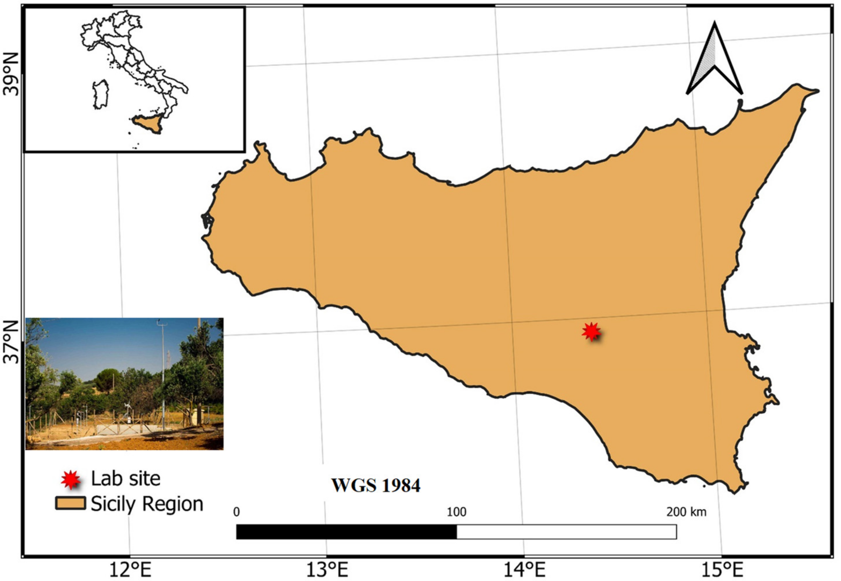
The proposed approach was applied to an experimental site located in Piazza Armerina (Sicily, Italy). The climate in this area is typically Mediterranean, with hot but not torrid summers, mild and short winters, and moderate annual rainfall mainly occurring in the period from October to March [74]. The annual average temperature along the coast is between 17 and 18.7 °C, with July being the hottest month [75]. The maximum (Tmax) and minimum temperature (Tmin), relative humidity (RH), wind speed (WS), and solar radiation (SR) data were obtained from Piazza Armerina meteorological station installed and managed by the Sicilian Agro-meteorological informative service (Servizio Informativo Agrometeorologico Siciliano—SIAS, http://www.sias.regione.sicilia.it/, accessed on 20 July 2022). The astronomical location of the meteorological site is 37.382171° N and 14.3666704° E, and its elevation is 697 m a.s.l. (Figure 1). The dataset consisted of 17.25 years of daily data covering the period from 1 December 2003 to 28 February 2021, for all variables.
3. Results
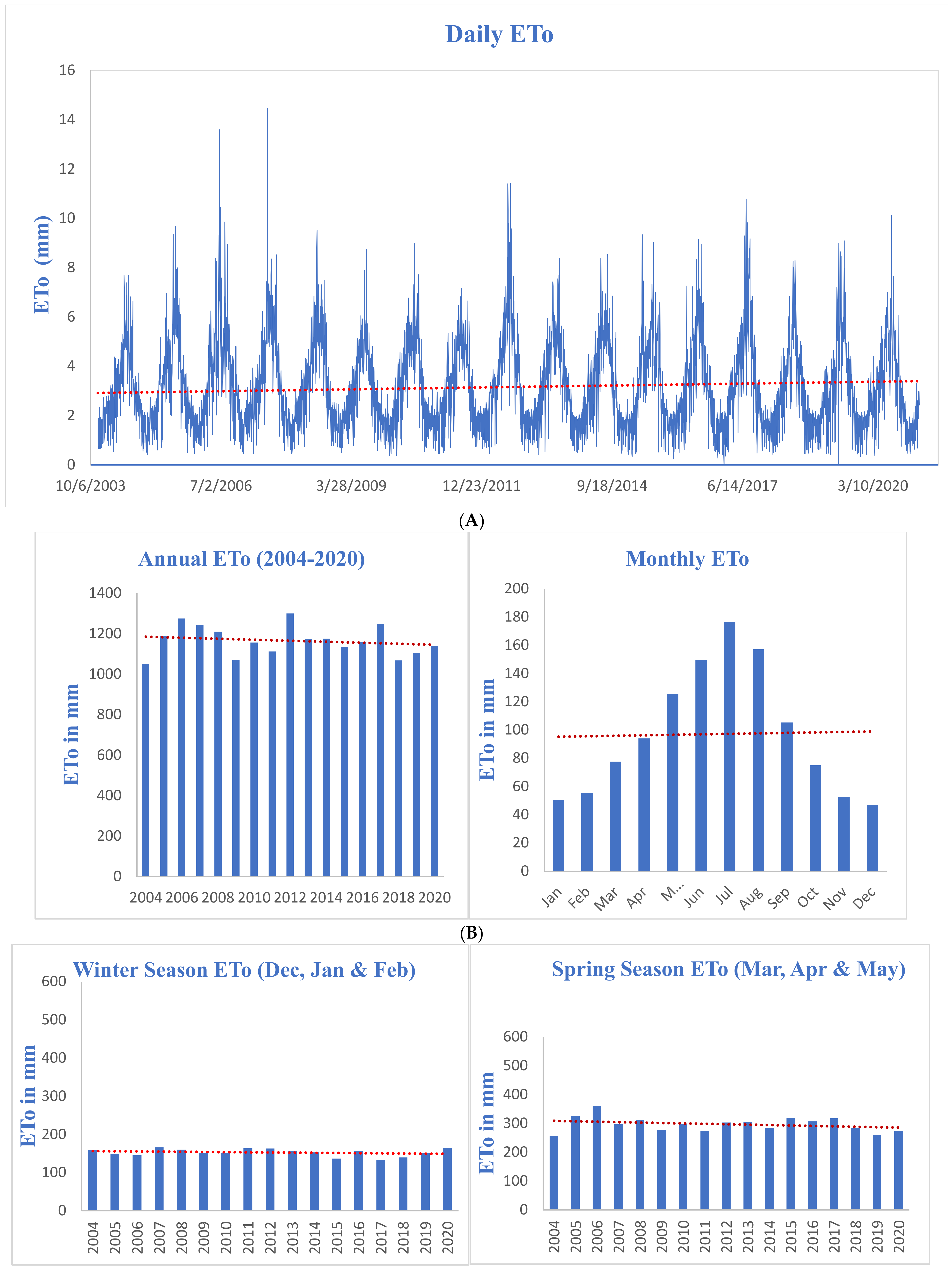
The Penman Monteith was applied for estimation of ETo in the 17-year timeframe of analysis. The result showed that maximum daily ETo was 14.47 mm per day on June 24, 2007 (Figure 2A), and the minimum daily ETo was 0.24 mm per day on 4 January 2016.
3.1. MK-Test Trends of Meteorological Factors and ETo
Table 2 shows the results concerning trend significance, as obtained from the MK-Test. The Tmax exhibits positive trends for March and September and spring and summer, while no significant trends were obtained for other time series. The Tmin presents positive monthly trends in August and September, and no other significant trends were observed. For Tmean, there was no significant trend except for September and spring and summer. Conversely, SR presents a negative trend in November and in Autumn. As regards WS, positive trends were observed on both seasonal and monthly scales. On the monthly scale, January, May, June, July, November, and December showed positive trends; for the remaining months no trend is evidenced. The HU also has a positive significant trend in March, April, May, June, July, August, September, October, and December, as well as in spring and summer. Rainfall showed a negative trend only in Autumn. The trend of ETo is negative only in November, and non-significant in the other cases.
3.2. Sen’s Slope (Magnitude of the Trend)
Climatic variables and ETo showed both negative and positive trends in seasonal and monthly scale analysis. The ETo showed a negative downward trend in November of 0.790 mm per year. The Tmax increased in March (0.10 °C) and September (0.14 °C) (monthly trend analysis), and spring (0.10 °C) and summer (0.09 °C) (seasonal trend analysis). The Tmin also increased in August (0.09 °C) and September (0.07 °C). The Tmean trend also increased in September (0.10 °C) in monthly analysis and in spring (0.07 °C), and summer (0.06 °C) in the seasonal analysis. The SR showed a downward trend in November (0.09 MJ/m2), at the monthly scale, and in Autumn (0.076 MJ/m2), at the seasonal scale. The WS also showed an upward trend in January (0.054 m/s), May (0.038 m/s), June (0.021 m/s), July (0.043 m/s), November (0.040 m/s), and December (0.042 m/s), as well as in winter (0.037 m/s) and spring (0.029 m/s). The HU trend also increased in March (0.711%), April (0.543%), May (1.169%), June (0.741%), July (1.012%), August (0.824%), September (0.816%), October (0.614%), and December (0.412%), as well as in spring (0.840%) and summer (0.942%). The RF also decreased in Autumn by 14.019 mm in the seasonal trend analysis.
3.3. Sensitivity of ETo to Climatic Factors
As the study stated above, for ETo estimation, Tmax, Tmean, Tmin, SR, WS, and SHU were used as input climatological variables. ETo showed different levels of sensitivity to these climatological variables. In particular, the result showed that SHU, Tmean, and Tmax have a very high sensitivity level, with sensitivity coefficients of 2.68, 1.46, and 1.35 respectively. The RS and Tmin also showed a high sensitivity level, with the sensitivity coefficient of 0.53 and 0.28 respectively. In contrast, the sensitivity level of wind speed was negligible, with a value of 0.02 for the sensitivity coefficient (Table 3).
3.4. Contribution Rate of Climatic Factors for the Variation of ETo
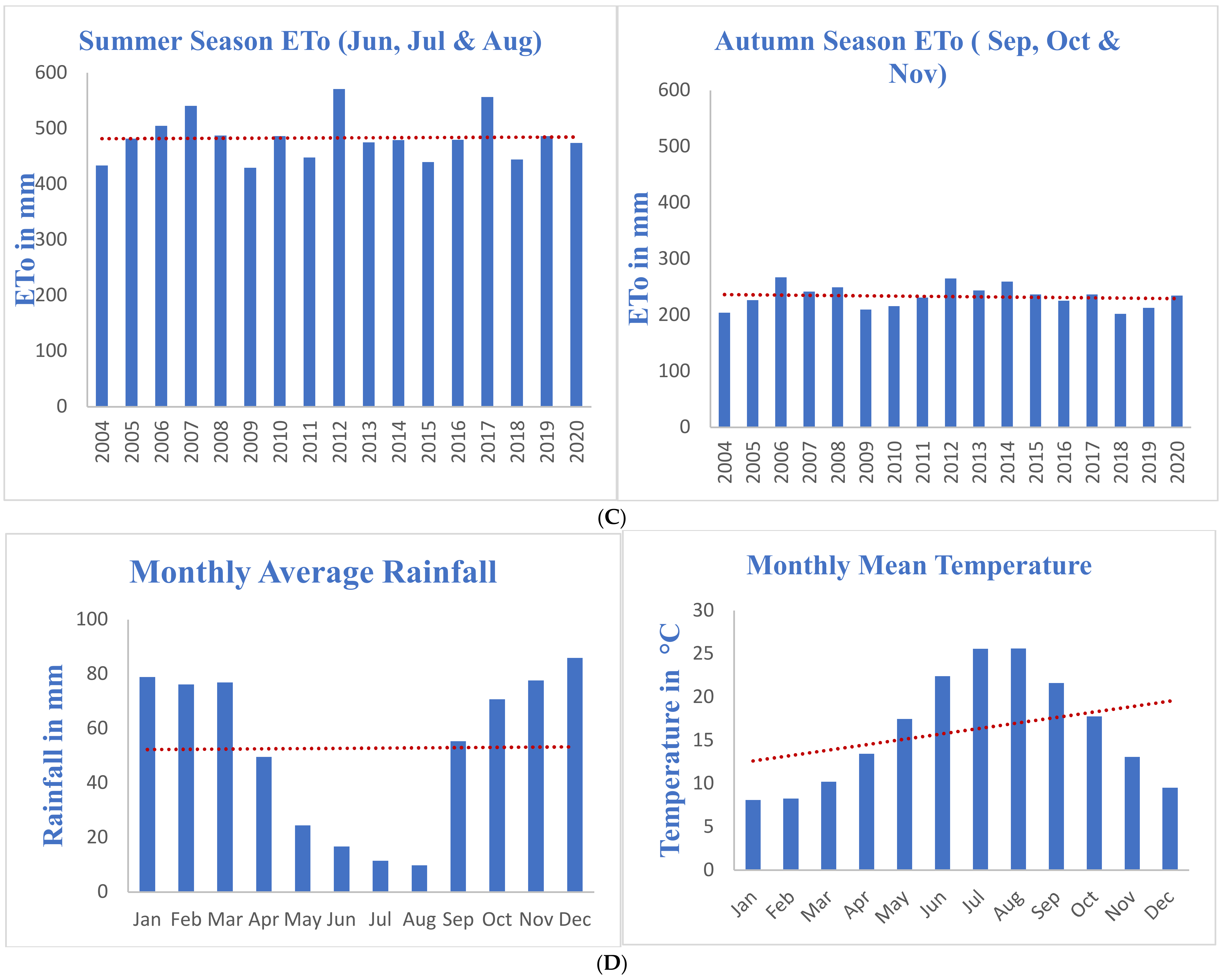
The above-mentioned climatic factors have different contribution rates for the ETo trends at different temporal scales. Figure 3 shows that the contribution rate of SHU, SR and Tmin are negative, with values of 91.73, 2.48, and 1.06, respectively. On the other hand, Tmax, Tmean, and WS contribute positively with an 11.2, 9.74, and 0.9 contribution rate. This result shows that SHU has the highest contribution to the decrease of ETo and maximum temperature has the highest contribution to the increase of ETo in the study area.
4. Discussion
4.1. Trend of Climatic Factors and ETo
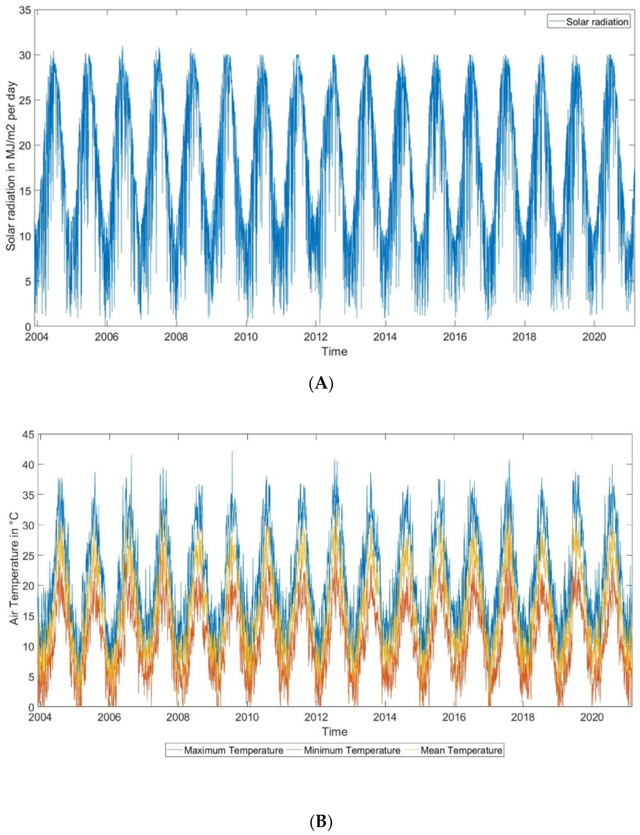
Globally, studies conducted by many authors showed that there is an upward trend of mean, maximum, and minimum temperature [76,77,78,79,80,81]. Our study also revealed that there were monthly and seasonal temperature upward trends at the experimental site in Sicily (Figure 4B). This is in line with similar research results showing an upward trend in temperature in Sicily [77,82]. The studies cited also showed a decreasing rainfall trend in autumn in Sicily. In particular, from 1921 to 2012 there was a downward trend of rainfall throughout the island in autumn [83] and a downward trend at the annual scale [39]. Moreover, a seasonal decrease in rainfall has been shown and documented in Sicily and Calabria [34]. Our study revealed that there was an increase in monthly and seasonal minimum temperature. Globally, in about the 37% of the landmasses from 1951–1990 the minimum temperature and maximum temperature increased by 0.84 °C and 0.28 °C respectively [84]. Similar results are also documented in several studies for different parts of Italy. From 1865 to 1996 southern Italy showed an upward trend of the minimum and maximum temperature, especially in southern Italy [85]. Moreover, from 1952 to 1990, Bologna showed an increase of 0.7 °C in 48 years in annual mean temperature and an increase in higher minimum and maximum temperature [86]. In Calabria (southern Italy), trend analysis results showed an increase in maximum and the minimum temperature specifically in the summer and spring seasons (from 1951 to 2010) [87]. This result is in line with our study since the maximum temperature showed a positive trend in summer and spring (Table 2). The maximum temperature also had a positive trend in Sardinia from 1982 to 2011 [88]. This study confirmed that there is an upward trend in mean temperature in summer, spring, and in the month of September (Table 2). The mean temperature of Sicily from 1924 to 2013 also showed an upward trend in summer and spring [82].
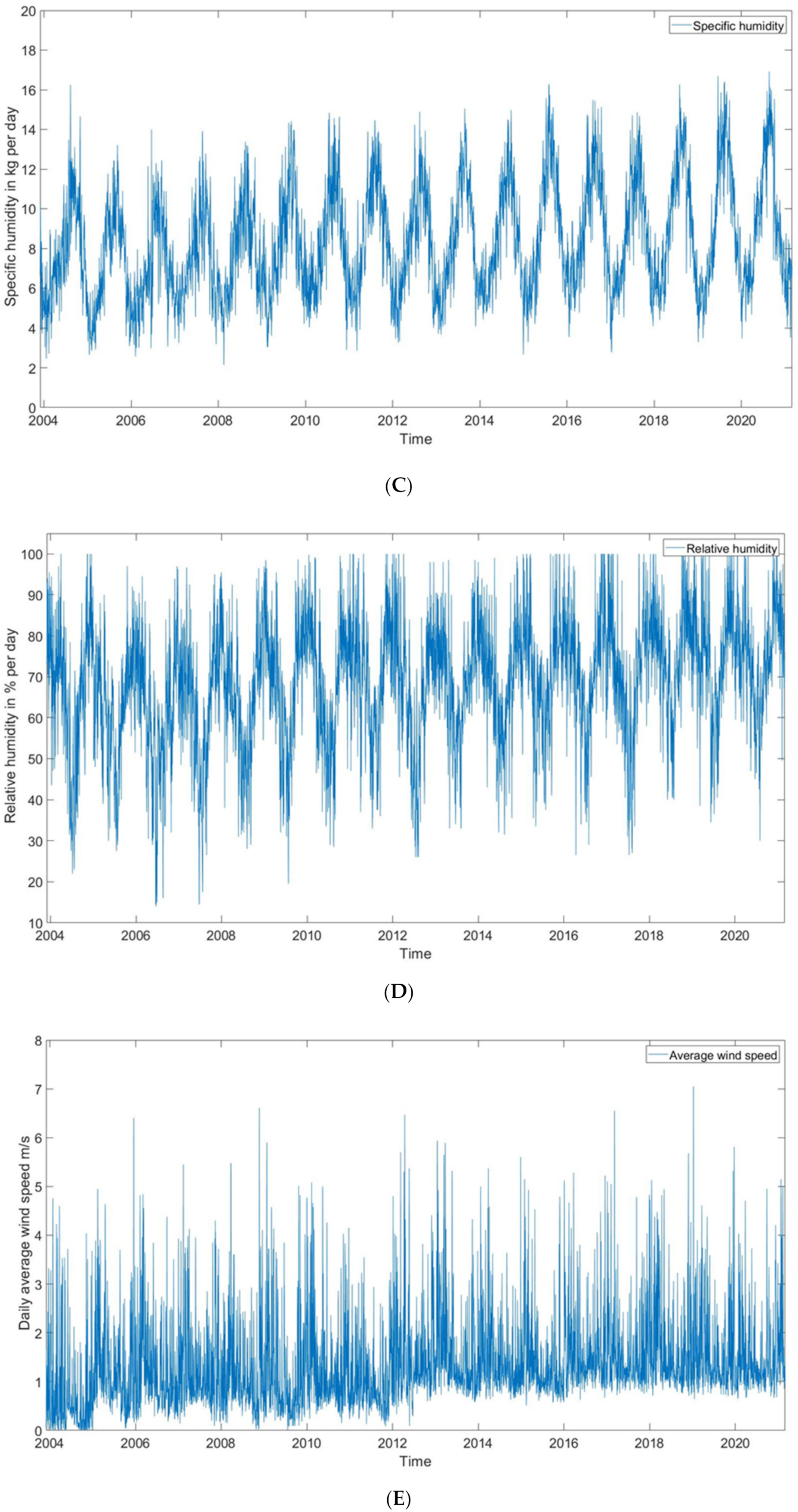
This study showed that there was increasing monthly and seasonal trend of relative humidity. In Ravenna, Italy, for the period 1989 to 2008, relative humidity had an upward trend [89]. Moreover, by considering the past and projected future data from 1971 to 2050, relative humidity also had an upward trend for Sicily [90]. Similar results showing an increase in relative humidity were confirmed in different part of the world [91,92,93]. Unlike other main meteorological factors, solar radiation showed a downward trend in November and in autumn (Table 2). Southern Italy showed a decrease in solar radiation after the mid-1980s [94]. In China from the 1960s to 2010s, solar radiation showed a downward trend [95,96]; and globally also showed a downward trend in solar radiation after the 1980s as well as the trend known as “global dimming” [97].
Like the most climatological elements, wind speed also showed an upward trend both in monthly and seasonal analysis (Table 2). Comprehensive studies that analyzed several meteorological sites showed both upward and downward trends in wind speed. Meanwhile, these studies also showed that there were increases in wind speed in monthly as well as seasonal timescales [98,99,100,101]. However, the study which analyzed 24 meteorological sites seasonal, monthly, and annually in Iran from 1975 to 2005 showed a downward trend in wind speed in most of its stations [92].
Table 2 showed that there was a downward trend in monthly reference evapotranspiration in November. This result is known as the “evaporation paradox”. There are many studies discussing a monthly, seasonal, and annual downward trend in ETo. For instance, studies conducted in China [25,66], India [38,69], and Senegal [36] revealed a downward trend in ETo seasonally, monthly, and annually. In Iran, a downward trend in seasonal and monthly trend was also found [27], and specifically in November [102]. In general, this study did not show seasonal or annual trends other than for November.
4.2. Sensitivity of ETo and Contribution Rate of Climatological Elements
The sensitivity analysis of ETo for climatic factors showed different magnitudes of sensitivity. The main and very high-level sensitivity in ETo trends was observed for specific humidity, mean temperature, and maximum temperature. Specific humidity was the most sensitive climatic factor for ETo trends in the study area. On the other hand, wind speed had a negligible sensitivity climatic factor for ETo trend. Likewise, relative humidity was the highest sensitivity climatic factor in the Loess Plateau of Northern Shaanxi, China [15]; in the Tao’er River Basin, China [71]; and in the Yellow River Basin, China [25]. Mean temperature was also one of the most sensitive factors for ETo in Iran [61]; in the Tarim River basin, in Central Asia [66] and in the Yellow River Basin, China [25].
Similarly maximum temperature was also the another prime sensitivity climatic factor for ETo in Senegal [36]; the Himalayan region of Sikkim, India [72]; the Tarim River basin, Central Asia [66], and in the Tons River Basin in Central India [69]. Wind speed also showed the lowest sensitivity in Santa Barbara [70]; the Himalayan region of Sikkim, India [72] and in the Tarim River basin, Central Asia [66].
This study showed that specific humidity, solar radiation, and minimum temperature contributed negatively to the trend of ETo; whereas maximum temperature, mean temperature, and wind speed contributed positively to ETo in the study area (Figure 3). The contribution values showed that the absolute value of the climatic factors showed the contribution magnitude. Hence specific humidity is the climatological factor that contributed the most to monthly decrease in ETo in November. On the other hand, wind speed made the least contribution to ETo in the study area. Maximum temperature was prominent in ETo in the Loess Plateau of Northern Shaanxi, in China and the Tarim River basin, in Central Asia; and wind speed was the factor that contributed less to ETo in the Loess Plateau of Northern Shaanxi, China [15].
5. Conclusions
In this study, referring to the FAO Penman-Monteith method for estimating reference evapotranspiration, we investigated the trends and sensitivity of ETo to meteorological variables. This analysis is important as there is a lack of similar studies. Also, in a climate change context it is key to understand the main climatological factors controlling such an important process for water resources management as evapotranspiration [103]. The analysis considered the data collected at a Mediterranean climate site in Sicily, Italy (Piazza Armerina). The results show that there was no annual trend for all the analyzed variables. Trends are present only at the sub-annual scale (monthly or seasonally). Significant trends at the monthly and seasonal time scales were exhibited for all variables other than minimum temperature and ETo. ETo showed a significant trend only monthly, for November (ETo), and minimum temperature only monthly, for August and September.
The sensitivity analysis also showed that specific humidity, mean temperature, and maximum temperature are those factors that have a greater influence on ETo. Sensitivity to wind speed is negligible. In terms of the contribution of the climatic factors for ETo trends, specific humidity, solar radiation, and minimum temperature contribute negatively to ETo. On the other hand, maximum temperature, mean temperature, and wind speed contribute positively. These results contribute to understanding the potential and possible future footprints of climate change on evapotranspiration in the study area. On the one hand, the fact that no significant trends are exhibited by ETo seems to imply that the impacts of climate change have not left a relevant footprint on this hydrological variable. On the other hand, given the high sensitivity of ETo to temperature, it must be expected that ETo will be highly impacted by climate change in the future; as temperature is expected to increase by 2–3 °C in Sicily, depending on emission scenario [104,105]. Moreover, the study in Pertouli and Taxiarchis in Greece also exhibited an increase in the potential evapotranspiration (PET) from 1974 to 2016 [106]. Further development of this study will consider more meteorological stations in Sicily, as well as other sources of data, to extend the length of the series and thus to improve the significance of trend assessments. Moreover, investigation could be extended, where data is available, to actual evapotranspiration.
Author Contributions
Conceptualization, T.M.A.; Formal Analysis, T.M.A. and D.J.P.; Funding Acquisition, G.S. and A.C.; Investigation, T.M.A.; Methodology, T.M.A.; Project Administration, A.G., G.S. and A.C.; Resources, G.S. and A.C.; Software, T.M.A.; Supervision, D.J.P., A.G. and A.C.; Validation, D.J.P.; Visualization, T.M.A. and D.J.P.; Writing—original draft, T.M.A. and D.J.P.; writing—review and editing, T.M.A., D.J.P. and A.G. All authors have read and agreed to the published version of the manuscript.
Funding
This study was supported by Ambiens srl. and the University of Catania 36th cycle funding scheme.
Institutional Review Board Statement
Not Applicable.
Informed Consent Statement
Not Applicable.
Data Availability Statement
Data generated during the present study are available from the corresponding author ([email protected]) upon reasonable request.
Acknowledgments
The author would like to thank the Ambiens srl. and the University of Catania for funding. Moreover, we would like to thank the SIAS service that provided 17 years of meteorological data.
Conflicts of Interest
The authors declare no conflict of interest.
References
- Ochoa-Sánchez, A.; Crespo, P.; Carrillo-Rojas, G.; Sucozhañay, A.; Célleri, R. Actual Evapotranspiration in the High Andean Grasslands: A Comparison of Measurement and Estimation Methods. Front. Earth Sci. 2019, 7, 139. [Google Scholar] [CrossRef] [Green Version]
- Glenn, E.P.; Nagler, P.L.; Huete, A.R. Vegetation Index Methods for Estimating Evapotranspiration by Remote Sensing. Surv. Geophys. 2010, 31, 531–555. [Google Scholar] [CrossRef]
- Zhang, F.; Liu, Z.; Zhangzhong, L.; Yu, J.; Shi, K.; Yao, L. Spatiotemporal Distribution Characteristics of Reference Evapotranspiration in Shandong Province from 1980 to 2019. Water 2020, 12, 3495. [Google Scholar] [CrossRef]
- Parajuli, K.; Jones, S.B.; Tarboton, D.G.; Flerchinger, G.N.; Hipps, L.E.; Allen, L.N.; Seyfried, M.S. Estimating actual evapotranspiration from stony-soils in montane ecosystems. Agric. For. Meteorol. 2018, 265, 183–194. [Google Scholar] [CrossRef] [Green Version]
- Ellsäßer, F.; Röll, A.; Stiegler, C.; Hendrayanto; Hölscher, D. Introducing QWaterModel, a QGIS plugin for predicting evapotranspiration from land surface temperatures. Environ. Model. Softw. 2020, 130, 104739. [Google Scholar] [CrossRef]
- He, D.; Liu, Y.; Pan, Z.; An, P.; Wang, L.; Dong, Z.; Zhang, J.; Pan, X.; Zhao, P. Climate change and its effect on reference crop evapotranspiration in central and western Inner Mongolia during 1961–2009. Front. Earth Sci. 2013, 7, 417–428. [Google Scholar] [CrossRef]
- Mueller, B.; Seneviratne, S.I.; Jimenez, C.; Corti, T.; Hirschi, M.; Balsamo, G.; Ciais, P.; Dirmeyer, P.; Fisher, J.B.; Guo, Z.; et al. Evaluation of global observations-based evapotranspiration datasets and IPCC AR4 simulations. Geophys. Res. Lett. 2011, 38, 6. [Google Scholar] [CrossRef] [Green Version]
- Long, D.; Singh, V.P. A Two-source Trapezoid Model for Evapotranspiration (TTME) from satellite imagery. Remote Sens. Environ. 2012, 121, 370–388. [Google Scholar] [CrossRef]
- Dickinson, R.E. Modeling Evapotranspiration for Three-Dimensional Global Climate Models. In Climate Processes and Vlimate Sensitivity; Geophysical Monograph Series; AGU Publishing: Washington, DC, USA, 1984; Volume 29, ISBN 9781118666036. [Google Scholar] [CrossRef]
- Dezsi, Ş.; Mîndrescu, M.; Petrea, D.; Rai, P.K.; Hamann, A.; Nistor, M.-M. High-resolution projections of evapotranspiration and water availability for Europe under climate change. Int. J. Clim. 2018, 38, 3832–3841. [Google Scholar] [CrossRef]
- Dong, Q.; Wang, W.; Shao, Q.; Xing, W.; Ding, Y.; Fu, J. The response of reference evapotranspiration to climate change in Xinjiang, China: Historical changes, driving forces, and future projections. Int. J. Clim. 2019, 40, 235–254. [Google Scholar] [CrossRef]
- Han, D.; Wang, G.; Liu, T.; Xue, B.-L.; Kuczera, G.; Xu, X. Hydroclimatic response of evapotranspiration partitioning to prolonged droughts in semiarid grassland. J. Hydrol. 2018, 563, 766–777. [Google Scholar] [CrossRef]
- Hui-Mean, F.; Yusop, Z.; Yusof, F. Drought analysis and water resource availability using standardised precipitation evapotranspiration index. Atmos. Res. 2018, 201, 102–115. [Google Scholar] [CrossRef]
- Kingston, D.G.; Todd, M.C.; Taylor, R.G.; Thompson, J.R.; Arnell, N.W. Uncertainty in the estimation of potential evapotranspiration under climate change. Geophys. Res. Lett. 2009, 36. [Google Scholar] [CrossRef] [Green Version]
- Li, G.; Zhang, F.; Jing, Y.; Liu, Y.; Sun, G. Response of evapotranspiration to changes in land use and land cover and climate in China during 2001–2013. Sci. Total. Environ. 2017, 596–597, 256–265. [Google Scholar] [CrossRef] [PubMed]
- Nam, W.-H.; Hong, E.-M.; Choi, J.-Y. Has climate change already affected the spatial distribution and temporal trends of reference evapotranspiration in South Korea? Agric. Water Manag. 2015, 150, 129–138. [Google Scholar] [CrossRef]
- Alemu, H.; Kaptué, A.T.; Senay, G.B.; Wimberly, M.C.; Henebry, G. Evapotranspiration in the Nile Basin: Identifying Dynamics and Drivers, 2002–2011. Water 2015, 7, 4914–4931. [Google Scholar] [CrossRef]
- Choudhary, D. Methods of Evapotranspiration; CCS Haryana Agricultural University: Hisar, India, 2018. [Google Scholar] [CrossRef]
- Gharsallah, O.; Facchi, A.; Gandolfi, C. Comparison of six evapotranspiration models for a surface irrigated maize agro-ecosystem in Northern Italy. Agric. Water Manag. 2013, 130, 119–130. [Google Scholar] [CrossRef]
- Hatfield, J.L.; Prueger, J.H.; Kustas, W.P.; Anderson, M.C.; Alfieri, J.G. Evapotranspiration: Evolution of Methods to Increase Spatial and Temporal Resolution. Am. Soc. Agron. 2016, 7, 159–193. [Google Scholar] [CrossRef]
- Tanner, C.B. Measurement of evapotranspiration. Irrig. Agric. Lands 1967, 11, 534–574. [Google Scholar]
- Moeletsi, M.E.; Walker, S.; Hamandawana, H. Comparison of the Hargreaves and Samani equation and the Thornthwaite equation for estimating dekadal evapotranspiration in the Free State Province, South Africa. Phys. Chem. Earth Parts A/B/C 2013, 66, 4–15. [Google Scholar] [CrossRef]
- Gul, S.; Ren, J.; Xiong, N.; Khan, M.A. Design and analysis of statistical probability distribution and non-parametric trend analysis for reference evapotranspiration. Peerj 2021, 9, e11597. [Google Scholar] [CrossRef]
- Tegos, A.; Malamos, N.; Koutsoyiannis, D. A parsimonious regional parametric evapotranspiration model based on a simplification of the Penman–Monteith formula. J. Hydrol. 2015, 524, 708–717. [Google Scholar] [CrossRef]
- Yang, Z.; Liu, Q.; Cui, B. Spatial distribution and temporal variation of reference evapotranspiration during 1961–2006 in the Yellow River Basin, China. Hydrol. Sci. J. 2011, 56, 1015–1026. [Google Scholar] [CrossRef] [Green Version]
- Gocic, M.; Trajkovic, S. Analysis of trends in reference evapotranspiration data in a humid climate. Hydrol. Sci. J. 2013, 59, 165–180. [Google Scholar] [CrossRef]
- Shadmani, M.; Marofi, S.; Roknian, M. Trend Analysis in Reference Evapotranspiration Using Mann-Kendall and Spearman’s Rho Tests in Arid Regions of Iran. Water Resour. Manag. 2011, 26, 211–224. [Google Scholar] [CrossRef] [Green Version]
- Ahmad, I.; Tang, D.; Wang, T.; Wang, M.; Wagan, B. Precipitation Trends over Time Using Mann-Kendall and Spearman’s rho Tests in Swat River Basin, Pakistan. Adv. Meteorol. 2015, 2015, 431860. [Google Scholar] [CrossRef] [Green Version]
- Kamal, N.; Pachauri, S. Mann-Kendall, and Sen’s Slope Estimators for Precipitation Trend Analysis in North-Eastern States of India. Int. J. Comput. Appl. 2019, 177, 7–16. [Google Scholar] [CrossRef]
- Blain, G.C. Removing the influence of the serial correlation on the Mann-Kendall test. Rev. Bras. Meteorol. 2014, 29, 161–170. [Google Scholar] [CrossRef] [Green Version]
- Zhang, F.; Geng, M.; Wu, Q.; Liang, Y. Study on the spatial-temporal variation in evapotranspiration in China from 1948 to 2018. Sci. Rep. 2020, 10, 17139. [Google Scholar] [CrossRef]
- Bouklikha, A.; Habi, M.; Elouissi, A.; Benzater, B.; Hamoudi, S. The Innovative Trend Analysis Applied to Annual and Seasonal Rainfall in the Tafna Watershed (Algeria). Rev. Bras. Meteorol. 2020, 35, 631–647. [Google Scholar] [CrossRef]
- Al Buhairi, M.H. Analysis of Monthly, Seasonal and Annual Air Temperature Variability and Trends in Taiz City-Republic of Yemen. J. Environ. Prot. 2010, 1, 401–409. [Google Scholar] [CrossRef] [Green Version]
- Caloiero, T.; Coscarelli, R.; Ferrari, E. Assessment of seasonal and annual rainfall trend in Calabria (southern Italy) with the ITA method. J. Hydroinformatics 2019, 22, 738–748. [Google Scholar] [CrossRef]
- Merabtene, T.; Siddique, M.; Shanableh, A. Assessment of Seasonal and Annual Rainfall Trends and Variability in Sharjah City, UAE. Adv. Meteorol. 2016, 2016, 6206238. [Google Scholar] [CrossRef] [Green Version]
- Ndiaye, P.; Bodian, A.; Diop, L.; Deme, A.; Dezetter, A.; Djaman, K.; Ogilvie, A. Trend and Sensitivity Analysis of Reference Evapotranspiration in the Senegal River Basin Using NASA Meteorological Data. Water 2020, 12, 1957. [Google Scholar] [CrossRef]
- Ghafouri-Azar, M.; Bae, D.-H.; Kang, S.-U. Trend Analysis of Long-Term Reference Evapotranspiration and Its Components over the Korean Peninsula. Water 2018, 10, 1373. [Google Scholar] [CrossRef] [Green Version]
- Sonali, P.; Kumar, D.N. Spatio-temporal variability of temperature and potential evapotranspiration over India. J. Water Clim. Chang. 2016, 7, 810–822. [Google Scholar] [CrossRef]
- Liuzzo, L.; Noto, L.V.; Arnone, E.; Caracciolo, D.; La Loggia, G. Modifications in Water Resources Availability Under Climate Changes: A Case Study in a Sicilian Basin. Water Resour. Manag. 2014, 29, 1117–1135. [Google Scholar] [CrossRef]
- Negm, A.; Jabro, J.; Provenzano, G. Assessing the suitability of American National Aeronautics and Space Administration (NASA) agro-climatology archive to predict daily meteorological variables and reference evapotranspiration in Sicily, Italy. Agric. For. Meteorol. 2017, 244–245, 111–121. [Google Scholar] [CrossRef]
- Negm, A.; Minacapilli, M.; Provenzano, G. Spatial disaggregation of POWER-NASA air temperatures and effects on grass reference evapotranspiration in Sicily, Italy. In EGU General Assembly Conference Abstracts; European Geosciences Union: Vienna, Austria, 2017; p. 13591. [Google Scholar]
- Borzì, I.; Bonaccorso, B.; Aronica, G.T. The Role of DEM Resolution and Evapotranspiration Assessment in Modeling Groundwater Resources Estimation: A Case Study in Sicily. Water 2020, 12, 2980. [Google Scholar] [CrossRef]
- Minacapilli, M.; Ciraolo, G.; Cammalleri, C.; D’urso, G. Evaluating actual evapotranspiration by means of mul-ti-platform remote sensing data: A case study in Sicily. IAHS-AISH Publ. 2007, 316, 207–219. [Google Scholar]
- Provenzano, G.; Ippolito, M. Using the ERA5 dataset of atmospheric variables to estimate daily reference evapotranspiration in Sicily, Italy. 4–5. In EGU General Assembly 2021; EGU: Vienna, Austria, 2021. [Google Scholar] [CrossRef]
- Aschale, T.M.; Sciuto, G.; Peres, D.J.; Gullotta, A.; Cancelliere, A. Evaluation of Reference Evapotranspiration Estimation Methods for the Assessment of Hydrological Impacts of Photovoltaic Power Plants in Mediterranean Climates. Water 2022, 14, 2268. [Google Scholar] [CrossRef]
- Consoli, S.; Russo, A.; Snyder, R. Estimating Evapotranspiration Of Orange Orchards Using Surface Renewal And Remote Sensing Techniques. AIP Conf. Proc. 2006, 852, 185–192. [Google Scholar] [CrossRef]
- Minacapilli, M.; Agnese, C.; Blanda, F.; Cammalleri, C.; Ciraolo, G.; D’Urso, G.; Iovino, M.; Pumo, D.; Provenzano, G.; Rallo, G. Estimation of actual evapotranspiration of Mediterranean perennial crops by means of remote-sensing based surface energy balance models. Hydrol. Earth Syst. Sci. 2009, 13, 1061–1074. [Google Scholar] [CrossRef] [Green Version]
- Willett, K.M.; Gillett, N.P.; Jones, P.D.; Thorne, P.W. Attribution of observed surface humidity changes to human influence. Nature 2007, 449, 710–712. [Google Scholar] [CrossRef]
- Hobbins, M.T. The Variability of ASCE Standardized Reference Evapotranspiration: A Rigorous, CONUS-Wide Decomposition and Attribution. Trans. ASABE 2016, 59, 561–576. [Google Scholar] [CrossRef] [Green Version]
- Nikam, B.R.; Kumar, P.; Garg, V.; Thakur, P.K.; Aggarwal, S.P. Comparative evaluation of different potential evapotranspi-ration estimation approaches. Int. J. Res. Eng. Technol. 2014, 3, 544–552. [Google Scholar]
- Alexandris, S.; Stricevic, R.; Petkovic, S. Comparative analysis of reference evapotranspiration from the surface of rainfed grass in central Serbia, calculated by six empirical methods against the Penman-Monteith formula. Eur. Water 2008, 21, 17–28. [Google Scholar]
- Almorox, J.; Senatore, A.; Quej, V.H.; Mendicino, G. Worldwide assessment of the Penman–Monteith temperature approach for the estimation of monthly reference evapotranspiration. Arch. Meteorol. Geophys. Bioclimatol. Ser. B 2016, 131, 693–703. [Google Scholar] [CrossRef]
- Chen, D.; Gao, G.; Xu, C.-Y.; Guo, J.; Ren, G. Comparison of the Thornthwaite method and pan data with the standard Pen-man-Monteith estimates of reference evapotranspiration in China. Clim. Res. 2005, 28, 123–132. [Google Scholar] [CrossRef]
- van der Schrier, G.; Jones, P.D.; Briffa, K.R. The sensitivity of the PDSI to the Thornthwaite and Penman-Monteith parame-teriza- tions for potential evapotranspiration. J. Geophys. Res. Earth Surf. 2011, 116, 1–16. [Google Scholar] [CrossRef]
- Seginer, I. The Penman—Monteith Evapotranspiration Equation as an Element in Greenhouse Ventilation Design. Biosyst. Eng. 2002, 82, 423–439. [Google Scholar] [CrossRef]
- Al-Sudani, H.I.Z. Derivation Mathematical Equations for Future Calculation of Potential Evapotranspiration in Iraq, A Review of Application of Thornthwaite Evapotranspiration. Iraqi J. Sci. 2019, 60, 1037–1048. [Google Scholar] [CrossRef]
- Anapalli, S.S.; Fisher, D.K.; Reddy, K.N.; Wagle, P.; Gowda, P.H.; Sui, R. Quantifying soybean evapotranspiration using an eddy covariance approach. Agric. Water Manag. 2018, 209, 228–239. [Google Scholar] [CrossRef]
- Kjelgaard, J.; Bellocchi, G. Evaluation of estimated weather data for calculating Penman-Monteith reference crop evapotranspiration. Irrig. Sci. 2004, 23, 39–46. [Google Scholar] [CrossRef]
- Hashemi, F.; Habibian, M. Limitations of temperature-based methods in estimating crop evapotranspiration in arid-zone agricultural development projects. Agric. Meteorol. 1979, 20, 237–247. [Google Scholar] [CrossRef]
- Quej, V.H.; Almorox, J.; Arnaldo, J.A.; Moratiel, R. Evaluation of Temperature-Based Methods for the Estimation of Refer-ence Evapotranspiration in the Yucatán Peninsula, Mexico. J. Hydrol. Eng. 2019, 24, 1040–1049. [Google Scholar] [CrossRef]
- Sharifi, A.; Dinpashoh, Y. Sensitivity Analysis of the Penman-Monteith reference Crop Evapotranspiration to Climatic Variables in Iran. Water Resour. Manag. 2014, 28, 5465–5476. [Google Scholar] [CrossRef]
- Subedi, A.; Chávez, J.L. Crop Evapotranspiration (ET) Estimation Models: A Review and Discussion of the Applicability and Limitations of ET Methods. J. Agric. Sci. 2015, 7, p50. [Google Scholar] [CrossRef] [Green Version]
- Allen, R.G.; Pereira, L.S.; Raes, D.; Smith, M. Crop Evapotranspiration-Guidelines for Computing Crop Water Requirements-Fao Irrigation and Drainage Paper 56; Fao: Rome, Italy, 1998; Volume 300, p. D05109. [Google Scholar]
- Peng, L.; Li, Y.; Feng, H. The best alternative for estimating reference crop evapotranspiration in different sub-regions of mainland China. Sci. Rep. 2017, 7, 5458. [Google Scholar] [CrossRef] [Green Version]
- Diop, L.; Bodian, A.; Diallo, D. Spatiotemporal Trend Analysis of the Mean Annual Rainfall in Senegal. Eur. Sci. J. ESJ 2016, 12, 231–245. [Google Scholar] [CrossRef]
- Wu, H.; Xu, M.; Peng, Z.; Chen, X. Temporal variations in reference evapotranspiration in the Tarim River basin, Central Asia. PLoS ONE 2021, 16, e0252840. [Google Scholar] [CrossRef]
- Hu, M.; Sayama, T.; Try, S.; Takara, K.; Tanaka, K. Trend Analysis of Hydroclimatic Variables in the Kamo River Basin, Japan. Water 2019, 11, 1782. [Google Scholar] [CrossRef] [Green Version]
- Sen, P.K. Estimates of the regression coefficient based on Kendall’s Tau. J. Am. Stat. Assoc. 1968, 63, 1379–1389. [Google Scholar] [CrossRef]
- Darshana; Pandey, A.; Pandey, R.P. Analysing trends in reference evapotranspiration and weather variables in the Tons River Basin in Central India. Stoch. Environ. Res. Risk Assess. 2012, 27, 1407–1421. [Google Scholar] [CrossRef]
- Irmak, S.; Payero, J.O.; Martin, D.L.; Irmak, A.; Howell, T.A. Sensitivity Analyses and Sensitivity Coefficients of Standardized Daily ASCE-Penman-Monteith Equation. J. Irrig. Drain. Eng. 2006, 132, 564–578. [Google Scholar] [CrossRef]
- Liang, L.; Li, L.; Zhang, L.; Li, J.; Li, B. Sensitivity of penman-monteith reference crop evapotranspiration in Tao’er River Basin of northeastern China. Chin. Geogr. Sci. 2008, 18, 340–347. [Google Scholar] [CrossRef]
- Patle, G.T.; Sengdo, D.; Tapak, M. Trends in major climatic parameters and sensitivity of evapotranspiration to climatic parameters in the eastern Himalayan region of Sikkim, India. J. Water Clim. Chang. 2019, 11, 491–502. [Google Scholar] [CrossRef]
- Lenhart, T.; Eckhardt, K.; Fohrer, N.; Frede, H.-G. Comparison of two different approaches of sensitivity analysis. Phys. Chem. Earth Parts A/B/C 2002, 27, 645–654. [Google Scholar] [CrossRef]
- Bonaccorso, B.; Cancelliere, A.; Rossi, G. Probabilistic forecasting of drought class transitions in Sicily (Italy) using Stand-ardized Precipitation Index and North Atlantic Oscillation Index. J. Hydrol. 2015, 526, 136–150. [Google Scholar] [CrossRef]
- Torina, A.; Khoury, C.; Caracappa, S.; Maroli, M. Ticks Infesting Livestock on Farms in Western Sicily, Italy. Exp. Appl. Acarol. 2006, 38, 75–86. [Google Scholar] [CrossRef] [PubMed]
- Jain, S.K.; Kumar, V. Trend analysis of rainfall and temperature data for India. Curr. Sci. 2012, 102, 37–49. [Google Scholar]
- Mohammad, P.; Goswami, A. Temperature and precipitation trend over 139 major Indian cities: An assessment over a century. Model. Earth Syst. Environ. 2019, 5, 1481–1493. [Google Scholar] [CrossRef]
- Mondal, A.; Khare, D.; Kundu, S. Spatial and temporal analysis of rainfall and temperature trend of India. Theor. Appl. Clim. 2014, 122, 143–158. [Google Scholar] [CrossRef]
- Saboohi, R.; Soltani, S.; Khodagholi, M. Trend analysis of temperature parameters in Iran. Theor. Appl. Clim. 2012, 109, 529–547. [Google Scholar] [CrossRef]
- Subash, N.; Sikka, A.K. Trend analysis of rainfall and temperature and its relationship over India. Theor. Appl. Clim. 2013, 117, 449–462. [Google Scholar] [CrossRef]
- Huss, M.; Farinotti, D.; Bauder, A.; Funk, M. Decadal trend of climate in the Tibetan Plateau—Regional temperature and precipitation. Hydrol. Process. Int. J. 2008, 22, 3056–3065. [Google Scholar]
- Liuzzo, L.; Bono, E.; Sammartano, V.; Freni, G. Long-term temperature changes in Sicily, Southern Italy. Atmos. Res. 2017, 198, 44–55. [Google Scholar] [CrossRef]
- Liuzzo, L.; Bono, E.; Sammartano, V.; Freni, G. Analysis of spatial and temporal rainfall trends in Sicily during the 1921–2012 period. Theor. Appl. Clim. 2015, 126, 113–129. [Google Scholar] [CrossRef]
- Jones, P. Maximum and minimum temperature trends in Ireland, Italy, Thailand, Turkey and Bangladesh. Atmos. Res. 1995, 37, 67–78. [Google Scholar] [CrossRef]
- Brunetti, M.; Buffoni, L.; Maugeri, M.; Nanni, T. Trends of Minimum and Maximum Daily Temperatures in Italy from 1865 to 1996. Theor. Appl. Clim. 2000, 66, 49–60. [Google Scholar] [CrossRef]
- Ventura, F.; Pisa, P.R.; Ardizzoni, E. Temperature and precipitation trends in Bologna (Italy) from 1952 to 1999. Atmos. Res. 2002, 61, 203–214. [Google Scholar] [CrossRef]
- Caloiero, T.; Coscarelli, R.; Ferrari, E.; Sirangelo, B. Trend analysis of monthly mean values and extreme indices of daily temperature in a region of southern Italy. Int. J. Clim. 2017, 37, 284–297. [Google Scholar] [CrossRef]
- Caloiero, T.; Guagliardi, I. Climate change assessment: Seasonal and annual temperature analysis trends in the Sardinia region (Italy). Arab. J. Geosci. 2021, 14, 2149. [Google Scholar] [CrossRef]
- Mollema, P.; Antonellini, M.; Gabbianelli, G.; Laghi, M.; Marconi, V.; Minchio, A. Climate and water budget change of a Mediterranean coastal watershed, Ravenna, Italy. Environ. Earth Sci. 2011, 65, 257–276. [Google Scholar] [CrossRef]
- Segnalini, M.; Bernabucci, U.; Vitali, A.; Nardone, A.; Lacetera, N. Temperature humidity index scenarios in the Mediterranean basin. Int. J. Biometeorol. 2012, 57, 451–458. [Google Scholar] [CrossRef]
- Abu-Taleb, A.A.; Alawneh, A.J.; Smadi, M. Statistical Analysis of Recent Changes in Relative Humidity in Jordan. Am. J. Environ. Sci. 2007, 3, 75–77. [Google Scholar] [CrossRef] [Green Version]
- Kousari, M.R.; Ekhtesasi, M.R.; Tazeh, M.; Naeini, M.A.S.; Zarch, M.A.A. An investigation of the Iranian climatic changes by considering the precipitation, temperature, and relative humidity parameters. Theor. Appl. Clim. 2010, 103, 321–335. [Google Scholar] [CrossRef]
- Huss, M.; Farinotti, D.; Bauder, A.; Funk, M. Changes in rainfall and relative humidity in river basins in northwest and central India. Hydrol. Process. Int. J. 2008, 22, 2982–2992. [Google Scholar]
- Manara, V.; Beltrano, M.C.; Brunetti, M.; Maugeri, M.; Sanchez-Lorenzo, A.; Simolo, C.; Sorrenti, S. Sunshine duration variability and trends in Italy from homogenized instrumental time series (1936-2013). J. Geophys. Res. Atmos. 2015, 120, 3622–3641. [Google Scholar] [CrossRef] [Green Version]
- Che, H.Z.; Shi, G.Y.; Zhang, X.-Y.; Arimoto, R.; Zhao, J.Q.; Xu, L.; Wang, B.; Chen, Z.H. Analysis of 40 years of solar radiation data from China, 1961–2000. Geophys. Res. Lett. 2005, 32. [Google Scholar] [CrossRef]
- Zhou, Z.; Wang, L.; Lin, A.; Zhang, M.; Niu, Z. Innovative trend analysis of solar radiation in China during 1962–2015. Renew. Energy 2018, 119, 675–689. [Google Scholar] [CrossRef]
- Ohmura, A. Observed decadal variations in surface solar radiation and their causes. J. Geophys. Res. Atmos. 2009, 114. [Google Scholar] [CrossRef] [Green Version]
- Eymen, A.; Köylü, U. Seasonal trend analysis and ARIMA modeling of relative humidity and wind speed time series around Yamula Dam. Meteorol. Atmos. Phys. 2018, 131, 601–612. [Google Scholar] [CrossRef]
- Jiang, Y.; Luo, Y.; Zhao, Z.; Tao, S. Changes in wind speed over China during 1956–2004. Theor. Appl. Clim. 2009, 99, 421–430. [Google Scholar] [CrossRef]
- Laib, M.; Golay, J.; Telesca, L.; Kanevski, M. Multifractal analysis of the time series of daily means of wind speed in complex regions. Chaos Solitons Fractals 2018, 109, 118–127. [Google Scholar] [CrossRef] [Green Version]
- Klink, K. Trends and Interannual Variability of Wind Speed Distributions in Minnesota. J. Clim. 2002, 15, 3311–3317. [Google Scholar] [CrossRef]
- Tabari, H.; Marofi, S.; Aeini, A.; Talaee, P.H.; Mohammadi, K. Trend analysis of reference evapotranspiration in the western half of Iran. Agric. For. Meteorol. 2011, 151, 128–136. [Google Scholar] [CrossRef]
- Peres, D.J.; Modica, R.; Cancelliere, A. Assessing Future Impacts of Climate Change on Water Supply System Performance: Application to the Pozzillo Reservoir in Sicily, Italy. Water 2019, 11, 2531. [Google Scholar] [CrossRef] [Green Version]
- Peres, D.J.; Senatore, A.; Nanni, P.; Cancelliere, A.; Mendicino, G.; Bonaccorso, B. Evaluation of EURO-CORDEX (Coordinated Regional Climate Downscaling Experiment for the Euro-Mediterranean area) historical simulations by high-quality observational datasets in southern Italy: Insights on drought assessment. Nat. Hazards Earth Syst. Sci. 2020, 20, 3057–3082. [Google Scholar] [CrossRef]
- Peres, D.J.; Bonaccorso, B.; Palazzolo, N.; Cancelliere, A.; Mendicino, G.; Senatore, A. Projected changes of hy-drologic variables and drought indices in southern Italy through an optimized Euro-CORDEX climate model ensemble weighted average. Hydrol. Sci. J. 2022; under review. [Google Scholar]
- Stefanidis, S.; Alexandridis, V. Precipitation and Potential Evapotranspiration Temporal Variability and Their Relationship in Two Forest Ecosystems in Greece. Hydrology 2021, 8, 160. [Google Scholar] [CrossRef]
Figure 1.
Location of the study area.

Figure 2.
Daily ETo (A), Annual ETo and Monthly ETo (B), Seasonal ETo (C), and Monthly Climatology (D).
Figure 2.
Daily ETo (A), Annual ETo and Monthly ETo (B), Seasonal ETo (C), and Monthly Climatology (D).


Figure 3.
Contribution of climatological factors to ETo.

Figure 4.
Daily timeseries of climate variables from December 1, 2003–December 28, 2021: (A–E) are Solar radiation, Air temperature (maximum, minimum, and mean temperature), Relative humidity, Specific humidity, and Wind speed, respectively.
Figure 4.
Daily timeseries of climate variables from December 1, 2003–December 28, 2021: (A–E) are Solar radiation, Air temperature (maximum, minimum, and mean temperature), Relative humidity, Specific humidity, and Wind speed, respectively.


Table 1.
Classification of the sensitivity coefficient.
| Sensitivity Coefficient | Sensitivity Level |
|---|---|
| 0.00 ≤ || < 0.05 | Negligible |
| 0.05 ≤ || < 0.2 | Moderate |
| 0.2 ≤ || < 1 | High |
| 1.00 ≤ || | Very high |
Table 2.
MK trend test result with 95% significance level.
| Jan | Feb | Mar | Apr | May | Jun | Jul | Aug | Sep | Oct | Nov | Dec | Win | Spr | Sum | Aut | Annual | |
|---|---|---|---|---|---|---|---|---|---|---|---|---|---|---|---|---|---|
| Tmax | 1.1 | 1.19 | 2.27 | 1.44 | 0.91 | 1.77 | 1.61 | 1.69 | 2.43 | 0.78 | 1.69 | 1.86 | 1.77 | 2.14 | 1.98 | 1.49 | 1.31 |
| Tmin | 0.08 | 0.95 | 0.99 | 0.62 | −0.49 | −0.21 | 1.19 | 2.18 | 2.14 | 0.01 | 1.36 | −0.37 | 0.12 | 0.33 | 1.03 | 1.4 | 1.19 |
| Tmean | 0.12 | 1.03 | 1.94 | 1.36 | 0.29 | 0.45 | 1.69 | 1.77 | 2.35 | 0.29 | 1.77 | 0.62 | 0.95 | 2.51 | 2.18 | 1.49 | 1.58 |
| SR | −0.95 | −0.54 | −0.7 | 0.62 | −1.65 | −0.33 | −0.78 | −1.2 | −1.07 | −1.44 | −2.02 | 0.95 | −0.12 | −0.87 | −0.91 | −2.6 | −1.44 |
| WS | 2.68 | 0.99 | 1.03 | 1.28 | 2.76 | 2.18 | 2.97 | 1.73 | 0.77 | 0.95 | 2.39 | 2.23 | 2.76 | 2.02 | 0.95 | 0.86 | 0.95 |
| HU | 0.41 | 0.5 | 2.27 | 2.27 | 2.12 | 2.84 | 3.17 | 2.39 | 2.12 | 2.02 | 1.22 | 2.02 | 0.86 | 2.21 | 2.03 | 1.31 | 1.31 |
| ETo | −1.85 | −0.95 | −1.11 | 0.45 | −1.28 | −0.62 | 0.54 | 0.21 | 0.45 | 0.04 | −2.51 | −0.95 | −0.54 | −0.78 | −0.21 | −0.54 | −0.78 |
| RF | −0.04 | 0.45 | −0.62 | −1.19 | 0.29 | −0.49 | 0.46 | 0.64 | −0.21 | 0.33 | 0.95 | 0.5 | −1.28 | −0.29 | −0.04 | −2.6 | −1.61 |
Win = winter; Spr = spring; Sum = summer; Aut = Autumn. Red color text = showed decreasing/upward trend.
Table 3.
Sensitivity coefficient of climatic factor for ETo.
| Climatological Element | Sensitivity Coefficient |x| | Sensitivity Level |
|---|---|---|
| Net solar radiation | |0.53| | High |
| Maximum temperature | |1.35| | Very high |
| Minimum temperature | |−0.28| | High |
| Mean temperature | |1.46| | Very high |
| Specific humidity | |−2.68| | Very high |
| Wind speed | |0.02| | Negligible |
Disclaimer/Publisher’s Note: The statements, opinions and data contained in all publications are solely those of the individual author(s) and contributor(s) and not of MDPI and/or the editor(s). MDPI and/or the editor(s) disclaim responsibility for any injury to people or property resulting from any ideas, methods, instructions or products referred to in the content. |
© 2023 by the authors. Licensee MDPI, Basel, Switzerland. This article is an open access article distributed under the terms and conditions of the Creative Commons Attribution (CC BY) license (https://creativecommons.org/licenses/by/4.0/).
Share and Cite
MDPI and ACS Style
Aschale, T.M.; Peres, D.J.; Gullotta, A.; Sciuto, G.; Cancelliere, A. Trend Analysis and Identification of the Meteorological Factors Influencing Reference Evapotranspiration. Water 2023, 15, 470. https://doi.org/10.3390/w15030470
AMA Style
Aschale TM, Peres DJ, Gullotta A, Sciuto G, Cancelliere A. Trend Analysis and Identification of the Meteorological Factors Influencing Reference Evapotranspiration. Water. 2023; 15(3):470. https://doi.org/10.3390/w15030470
Chicago/Turabian StyleAschale, Tagele Mossie, David J. Peres, Aurora Gullotta, Guido Sciuto, and Antonino Cancelliere. 2023. "Trend Analysis and Identification of the Meteorological Factors Influencing Reference Evapotranspiration" Water 15, no. 3: 470. https://doi.org/10.3390/w15030470
Note that from the first issue of 2016, this journal uses article numbers instead of page numbers. See further details here.