
Parametrization of Eddy Mass Transport in the Arctic Seas Based on the Sensitivity Analysis of Large-Scale Flows

Institute of Computational Mathematics and Mathematical Geophysics, SB RAS, 630090 Novosibirsk, Russia
*
Author to whom correspondence should be addressed.
Water 2023, 15(3), 472; https://doi.org/10.3390/w15030472
Submission received: 10 December 2022
/
Revised: 14 January 2023
/
Accepted: 17 January 2023
/
Published: 25 January 2023
(This article belongs to the Special Issue Research on Fluid Flows: Modelling, Numerical Simulations, and Computational Dynamics)
Abstract
:The characteristics of eddy mass transport are estimated depending on the values of the parameters of a large-scale flow that forms under the conditions of the shelf seas in the Arctic. For this, the results of numerical simulation of the Kara Sea with a horizontal resolution permitting the development of mesoscale eddies are used. The multiple realizations of eddy mass flux resulting from a numerical experiment are considered as a statistical sample and are analyzed using methods of sensitivity study and clustering of sample elements. Functional dependencies are obtained that are closest to the simulated distributions of quantities. These expressions make it possible, within the framework of large-scale models, to evaluate the characteristics of the cross-isobathic eddy mass transport in the diffusion approximation with a counter-gradient flux. Numerical experiments using the SibCIOM model showed that areas along the Fram branch of the Atlantic waters trajectory in the Arctic as well as the shelf of the East Siberian and Laptev seas with adjacent deep water areas are most sensitive to the proposed parametrization of eddy exchanges. Accounting for counter-gradient eddy fluxes turned out to be less important.
1. Introduction
One of the most important tasks in large-scale modeling of the oceans in the framework of climate models is an adequate description of subgrid-scale processes, that is, processes that, with the accepted horizontal and vertical resolution of the model, as well as due to some simplifying assumptions, cannot be explicitly described by a numerical solution of the relevant set of differential equations. In such cases, one can resort to a parametric description of the large-scale consequences of such mesoscale processes.
Among these processes is the eddy transport of scalar quantities. The scales of eddy formations in the ocean vary in a fairly wide range, and not all of them can be properly described. However, the result of the action of such mesoscale (and submesoscale) eddies, namely the exchange of properties of the waters involved in the movement, requires a search for additional possibilities for the parametrization of these processes.
The most common method is the parametrization of eddy fluxes using diffusion approximation when large-scale diffusion fluxes are enhanced by a specially chosen diffusion coefficient. A uniform increase in the diffusion coefficient leads to a smoothing of the thermodynamic characteristics of the ocean, including cases of absent or weak eddy motion. A more differentiated approach is associated with the introduction of the diffusion coefficient being variable in space and time. However, the question arises of how to recognize the presence or absence of an eddy activity with only large-scale flow characteristics on hand. For example, in his approach, Smagorinsky [1] uses the presence of sheer and divergence in the velocity field to calculate the viscosity coefficient associated with mesoscale eddies.
Eddy diffusion and viscosity models are introduced into the coarse models to simulate unresolved eddy-driven motions. This mechanism is often represented by some functional statements [2,3] that depend on the resolved flow properties.
The most used parametrization of the mesoscale effect is based on the eddy advection scheme [4,5,6], which consists in simulating the effect of baroclinic instability by flattening the isopycnal surfaces, which transfers available potential energy toward the eddy kinetic energy of subgrid-scale motions. However, such a scheme reduces the total energy, since it does not take into account the reverse transfer of kinetic energy to large scales [7]. Usually, the development of parametrization schemes and the evaluation of their parameters occur regardless of the climate models in which they are eventually to be included. They are tested in field experiments and the test area is relatively small compared to the area covered by large-scale climate models. In addition, parametrizations usually contain uncertain parameters, that is, there is parametric and structural uncertainty [8].
After parametrization schemes are developed and included in a climate model, modelers tune the parameters to make the model adequately simulate the known physical processes and/or their observations [9]. Recently, to tune parameters, modelers use data-driven algorithms. This is due to big data accumulation and the rapid development of methods for processing them, including data assimilation methods [10,11], as well as machine learning [12] and statistical [13] methods. A whole class of data-driven parametrizations has emerged [14,15], rather than using idealized theories. Statistical methods are also traditionally used to manage and analyze data. They can be used to integrate high-resolution targeted local modeling into a large-scale climate model, systematically learning from the results of the local model and quantifying uncertain parameters of large-scale modeling.
This article proposes to use the results of regional modeling based on a model that resolves mesoscale eddies and well-known statistical approaches to analyze the sensitivity of eddy fluxes to the characteristics of large-scale motion. Based on this approach, an attempt will be made to obtain a functional dependence of the eddy transport characteristics on large-scale ocean thermodynamic characteristics using the Kara Sea shelf model in the Arctic as an example. In recent studies, a similar approach was used in [16,17,18] but the eddy-diffusivity/mass-flux approach (EDMF) was applied to parameterize convection and planetary boundary layer in atmospheric models.
Finally, the obtained expressions for the parametrization dependences were used in the framework of large-scale modeling of processes in the Arctic and the North Atlantic using the Siberian Coupled Ice-Ocean Model (SibCIOM). With its help, it was possible to evaluate the model sensitivity to the developed parameters and identify the main trends in the simulated state of the ocean, associated with the inclusion of cross-isobathic eddy flows in such large-scale models of the Arctic region.
Section 2 is devoted to the description of the high-resolution model (Section 2.1) and the analysis methods used when considering the simulation results. The type of parametrization used for eddy mass transport is described in Section 2.2. Section 2.3 describes a method for estimating large-scale flow characteristics using high-resolution simulation results. The list of considered large-scale characteristics that can be used for the parametrization of eddy mass transport is given in Section 2.4, and Section 2.5 contains the results of a study on the statistical independence of these characteristics, estimated in the analysis of a sample prepared from the simulation results. Section 2.6 describes a method for clustering sample elements, the purpose of which is to isolate groups of eddy transport realizations obtained under the action of physically different mechanisms. Finally, Section 2.7 describes the algorithm for studying the dependence of eddy mass transport parameters on large-scale flow characteristics. For introductory reading, some of these sections can be skipped because they contain many less significant details.
The results of the study are given in Section 3. First of all, the results of the clustering of the sample elements in Section 3.1 are considered. Then, in Section 3.2, based on the sensitivity analysis, one-dimensional dependences of the eddy mass transport parameters on the most significant flow characteristics are derived. One of the variants of applying the obtained parametrizations in a large-scale model is described in Section 3.3, and Section 3.4 and Section 3.5 describe the results of applying the obtained parametrizations of eddy diffusion and eddy counter-gradient transport, respectively, in modeling the Arctic and the North Atlantic in the period 2000–2022 using the SibCIOM large-scale model.
Section 4 discusses the results obtained and concludes.
2. Materials and Methods
2.1. The Model of the Kara Sea
SibPOM sigma coordinate shelf model [19,20], which is a modification of the Princeton Ocean Model (POM) [21], was used as a regional high-resolution model. It includes the parametrization of vertical turbulent processes and the correction of the horizontal pressure gradient error due to the sigma coordinate [22]. The simulation area is shown in Figure 1. The quasi-regular grid of the region is constructed based on a rotated spherical coordinate system with the poles selected so that the new equator is the central axis of the Kara Sea. The horizontal resolution is chosen high enough to reproduce large mesoscale eddies, according to [23].
The Kara Sea model is nested in the Arctic and North Atlantic coupled ice–ocean model SibCIOM [24]. The model embedding scheme is given earlier in [19]. The main idea is that the Laplace operator, which describes the thermal conductivity and diffusion of the salt in a high-resolution model, was applied only to deviations of temperature and salinity from their large-scale distributions. Feedback in this case was not taken into account.
The results discussed below refer to a numerical experiment covering the period from September 2006 to September 2008, the results of which were presented in our previous paper [20]. From this experiment, only 2007 was taken into account in our analysis below. Thus, we expected to incorporate the extremal features of this year when considering cross-isobathic transport.
2.2. Parametrization of Cross-Isobathic Transport
The horizontal transport of density fluctuations by velocity fluctuations is described by the terms in the mass conservation equation of the form
where is the horizontal velocity fluctuation vector with components , and are the regular components of the horizontal current velocity, that is, the averaged velocity components over a certain characteristic period of time T. Accordingly, the operator is the result of averaging the value over this time period. Thus, the mass flux in the direction of some vector is defined as follows
In our numerical experiment with a detailed resolution, the time-averaged values of both components and along with the value of the density at each point of the grid area, as well as the time-averaged values of the flux components and , were each stored for 12 h periods. Thus, any averaging period can be chosen with a resolution of 12 h, that is, from 12 h to several days. The time scale T characterizing the time of the influence of the mesoscale eddy on the state of the ocean at a certain point is about 10 days [25]. Therefore, hereafter we will consider 10 days (averaging from the 1st to the 10th day of the month, from 11th to 20th, and from 21st to the end of the month), that is, about 20 12 h records will be used for the averaging operation . The most interesting direction of mass transport carried out by mesoscale eddies is the direction perpendicular to the geostrophic flow, that is, locally this direction coincides with the direction of ocean depth growth . Within the framework of the diffusion approximation, such an eddy flux is parameterized using large-scale characteristics in the form [26,27,28]
using the eddy diffusion coefficient K and the counter-gradient , due to which the counter-gradient flux is formed. Such a flux is formed in the absence of a change in density in the direction of the vector due to an ordered vortex structure. To calculate the large-scale horizontal averaging, we will use a scale of 50 km, since this approximately corresponds to the grid spacing of the large-scale model. The horizontal averaging of a certain value will be denoted by angle brackets . It means the value at some point , which is obtained by averaging over all points of the model with a detailed resolution located in the square . Thus, the values K and q can be found using the least squares method as linear regression coefficients
that is
The application of Formulas (4)–(6) is limited by the fact that as a result of calculations the value of the eddy diffusion coefficient K may turn out to be negative, which causes instability of the solution of the system equations. Therefore, in the following analysis, we will consider only those implementations for which the use of the expression (3) does not lead to instability, namely those implementations when the value of K obtained by Formulas (4)–(6) takes non-negative values.
2.3. Large-Scale Representation of Mesoscale Characteristics
Any value can be represented as its linearization in the vicinity of a point in horizontal coordinates in the form
where the coefficients A, B, and C can also be found by the least squares method, i.e.,
where the following operator is introduced as a notation
As before, the designation here means such a value of the characteristic at the point , which is obtained by its averaging over all points of the model with a detailed resolution located in the square .
2.4. Large-Scale Flow Characteristics
The purpose of our analysis is to single out among the large-scale characteristics those on which the eddy mass transport in the cross-isobathic direction depends to a greater extent. That is, taking into account the parametrization dependence (3), we aim to find out on which large-scale characteristics of the flow the values K and q depend to the greatest extent. Table 1 presents a list of considered geographic and physical characteristics.
For each of these values at each grid point of the high spatial resolution model, the corresponding large-scale value can be found by using and operators described previously. Based on the results of modeling the Kara Sea using the SibPOM [20,29] model, about 78 million records of these values and the corresponding values of K and q were obtained. However, later on, the seven most independent values were selected out of sixteen values (see below).
2.5. Independence of Large-Scale Characteristics
It will be further assumed that K and q are functions of several large-scale characteristics. The sensitivity analysis of K and q to these characteristics provides for their statistical independence from each other. That is, 16 selected characteristics will be considered as 16 independent variables on which the value of these functions depends. An analysis of the 78 million records mentioned earlier showed that, based on the Fisher test, none of these variables are independent. Even latitude and longitude are not statistically independent because, for example, due to the shape of the basin, latitude cannot take on certain values at some fixed longitudes. The same applies to local depth z. However, it was possible to rule out the characteristics that are most dependent on others (see Table 1):
- The depth of the ocean H, in situ depth z, vertical component of in situ density gradient , and geographical latitude turned out to be strongly related to each other. Among them, the most prominent physical meaning has value as it defines the Brunt–Väisälä frequency of internal waves.
- The flow velocity in the direction of slope U, the component of the in situ density gradient in the direction of the slope turned out to be strongly related to the value of this characteristic near the bottom . Among them, we chose the latter, because according to [30], it is an important characteristic of cascading.
- Similarly, the near-bottom density gradient component along the isobath turned out to be strongly dependent on the in situ value of this gradient , so this value was neglected in favor of the second one.
- The flow velocity in the direction along the isobaths V turned out to be dependent on the down-slope component of the bottom density gradient , which is already chosen.
- The divergence of the velocity components and are related by the continuity equation, we chose the latter one of them.
The coordinates , , z, and, in addition to them, time t, are, in principle, independent variables. All others are functions of them. Nevertheless, they were neglected, since it is better to deal with physical state characteristics, because if we consider just these four we could not extend this dependence beyond the domain of the Kara Sea model or beyond 2007.
As a result, the following seven values in the large-scale approximation were considered as variables on which the values K and q can depend: s, , , , , , and .
2.6. Clustering
The total sample, built on the results of a high-resolution simulation, contains elements consisting of a set of parameters characterizing the large-scale motion
and parameters describing the integral effect of mesoscale pulsations on the large-scale motion . Since the specified set of characteristics could be attributed to completely different mesoscale movements, such as baroclinic and barotropic instabilities, cascading, and convection, amongst others, and refer to corresponding physical mechanisms, it makes sense to divide the entire sample into clusters, that is, into groups of the most closely related sample elements in the same way as in [31,32].
There are several approaches related to the choice of criterion for the tightness of the connection between elements. In this study, the so-called k-means method was used [33], in which belonging to a cluster is determined by the fact that the distance to its center is minimal among the centers of all clusters. The clustering procedure is iterative, after determining the belonging of elements to clusters, the center of each cluster is redefined according to the elements included in it. The iterations stop as soon as the composition of the clusters becomes unchanged.
An important issue in the implementation of the k-means method is the choice of the number of clusters k and the initial position of their centers. The choice of the number of clusters is based on the fact that the number of sources of mesoscale motions is not large. They include barotropic or baroclinic instabilities in the region of jet streams or near density fronts, as well as in regions of intense convective and wind mixing. Having considered the values of k from 2 to 8 as options, it was decided to stop at the value of , since the resulting clusters, in this case, are more cohesive according to the relevant criteria, and also have a clear geographical localization, indicating a corresponding physical nature, such as river plume eddies and steep slope eddies (see below). Clusters could differ in volume because their elements form separate compact groups in a 7D area. Some of these groups could be large, others could be small. The k-means clustering principle is to find distant groups of elements. Geometrically, it means that the 7D distances between elements in each of the groups are smaller than distances between groups.
In general, the values of the parameters characterizing the large-scale movement is a vector in N-dimensional space, where N is equal to the number of these parameters (in our case, ). Since the parameters are heterogeneous in nature, normalization is used to achieve their equivalence; that is, instead of a vector , a modified vector is used, where
and
M is the length of the sample, is the value of the i-th parameter in the j-th element of the sample. After normalization, the coordinates of the center of the l-th cluster are defined as
where is the set of sample elements belonging to the l-th cluster, is the number of these elements, is the value of the normalized i-th parameter in the j-th sample element. After finding the centers of clusters, the belonging of the sample elements to the clusters is redefined as
if
The initial position of the cluster centers is determined by following the k-means++ [34] algorithm:
- The center of the first cluster is determined randomly.
- The center of the second cluster is determined randomly with a probability proportional to the distance to the center of the first cluster.
- The center of the next i-th cluster is also determined randomly with a probability proportional to the minimum among the distances to the known cluster centers.
Conventional indices are used to determine the quality of clustering and search for the most appropriate partition (Appendix A, Appendix A.1, Appendix A.2 and Appendix A.3).
2.7. Analysis of Dependencies on the Selected Parameters
The values of eddy diffusion coefficient K and counter-gradient flux q resulting from high-resolution simulations vary in a fairly wide range. The variability of the K value is several orders of magnitude. Therefore, to narrow the range, the logarithm of this value was considered, and made dimensionless with the help of some characteristic value ; thus, instead of the eddy diffusion coefficient, the value was considered, while only the values of m/s were taken into account. The variability of the counter-gradient eddy flux q is also several orders of magnitude and, at the same time, has both positive and negative values in a comparable proportion. In addition, it takes most of the values in a fairly narrow range. Therefore, to isolate the region of the most frequent values of the characteristic, instead of the eddy flux itself, the following function was considered where is the sample mean value of the flux, and is its standard deviation. The use of hyperbolic tangent narrows the range of values to the segment , while the values in the central part, represented by the overwhelming number of sample elements, experience only a linear normalization transformation.
Following the Sobol’ method [35,36], we represent the dependence of the value or on the N parameters of the large-scale model in the form
where
Here, E denotes the mathematical expectation of the value obtained as a result of the statistical evaluation, and denotes the Y value at fixed ,…values. According to [35], the values are assumed to be uniformly distributed over the interval [0, 1]. Therefore, we will divide the entire range of changes into L boxes with an equal number of elements in each of them. Thus, after clustering is performed, to apply the Sobol’ sensitivity analysis, as values, we can consider values that are discrete on a segment and obtained as a result of the distribution of elements over L successive intervals or boxes each containing of the sample elements.
3. Results
3.1. Clustering Results
Since the process of selecting clusters is random at the stage of the initial separation, the result may not be optimal. Therefore, for each k value from 2 to 8 clusterings were carried out, from which the variant with the optimal values of the above indices was selected. Naturally, under such conditions, we are still not guaranteed that the partition will be optimal, but the chance of optimality increases significantly. From the analysis of the resulting partitions, it follows that the process of selecting clusters has about 2–3 limit states, so choosing the most optimal one is not a problem.
Table 2 presents the results of the performed clusterings with the number of clusters identified from to 5, and Figure 2 and Figure 3 show the geographical location of elements of these clusters: Figure 2 presents the number of elements in whole vertical column for each model grid cell and Figure 3 shows their depth-latitude distribution by means of blue dots. Only elements with m/s are considered. The table shows that in the case of selecting two clusters, their size (the number of elements in them) differs by an order of magnitude. A large cluster is presented, covering 91% of all elements, and a small one, including 9% of the elements. Geographically, the former is distributed throughout the entire Kara Sea basin over the entire range of depths. The second is localized in the coastal part in the places where the waters of Siberian rivers spread, and vertically, it is located in the upper layer within a few tens of meters. The latter, in our opinion, indicates that the elements of this cluster correspond to a set of parameters that describe the specifics of the distribution of the river plume and the development of the salinity front in the upper layer of the sea. Different number of elements in clusters is related to a small number of grid nodes representing the river plume compared to others. Geometrically, it means that these elements are distant from others in a 7D space area, at least in terms of variables representing the vertical components of density gradient.
With an increase in the number of clusters to three, the previously mentioned cluster with river influence remains practically unchanged and makes up the same 9% of the elements. For brevity, we will denote this cluster as B. An even smaller cluster, covering only 3%, is separated from the large cluster. We will mark it with the symbol C. Thus, the number of elements in the largest cluster has decreased to 88%. This cluster will be marked by the symbol A. Cluster C turned out to be geographically localized in a narrow strip of the steepest slope at the boundary between the shelf and the deep ocean and its elements are distant in the 7D space area from others, at least due to the extremely large s variable. Thus, this cluster contains elements with parameters that describe the specifics of mesoscale movements in the region of a steep shelf slope. This partition has the smallest Davies–Bouldin index among the considered ones and the largest Dunn index, which indicates its optimality according to these criteria (see index descriptions in Appendix A.1, Appendix A.2 and Appendix A.3). Its silhouette coefficient turned out to be somewhat smaller compared to splitting into two clusters (0.74 instead of 0.78), but the silhouette coefficient of the largest cluster slightly increased from 0.95 to 0.96. This partition will be further considered as the main one.
An increase in the number of clusters to four and five leads to the formation of an intermediate cluster associated with the upper layer being no deeper than 100 m, due to a decrease in the proportion of the large cluster A and the proportion of the river cluster B, the latter becomes the smallest as a result and covers the areas immediately adjacent to the river mouths. Our interpretation of the intermediate cluster is to identify areas of convective and wind mixing. In addition, a large cluster also splits into two, while part of the intermediate cluster is captured. As a result, a reduced version is formed from its remaining part. Also, with an increase in the number of clusters the quality of clustering decreases. We also checked 25 clustering, which also proves a further quality decrease.
The introduced designations of clusters for reference are presented in Table 2.
3.2. Parametrization Dependencies—Cluster A
We restrict our analysis of the resulting partition to the consideration of the largest obtained cluster A, leaving consideration of other clusters and other partitions for future research.
The dependence of the eddy diffusion coefficient K on large-scale parameters was estimated based on dividing the variability ranges of each of the parameters into successive intervals with an equal number of sample elements in them. Dividing by more intervals results in a lot of computations when evaluating sensitivity because the number of boxes in N-dimensional hyperspace is . In the considered case their number is = 78,125.
Cluster A covers 88% of all sample elements. The coefficient of eddy diffusion K in the representation of eddy mass transport (3) revealed the strongest dependence on the value of the vertical derivative of the density, which is related to the Brunt–Väisälä frequency by the relation
This value is involved in explaining 69% of the variability in the value in this cluster.
The second most important value is the rate of density change along the direction of the bottom slope, which is responsible for 47% of the variability. The third value, which explains 39% of the variability, is the rate of the bottom slope. It is from these values that the individual dependence of the value on one-dimensional functions in representation (18) is most pronounced: – 33.4%, – 7.6%, and s – 1.7%. The distributions of the cluster elements against these values are presented in Figure 4 using histograms in terms of their normalized deviations from the mean. The role of other parameters in explaining the dependence is not negligible and varies from 24 to 33%. Among the two-dimensional functions, the most pronounced dependence on pairs of variables is – 3% and – 1.3%. For multivariate functions, it can be noted that any combination of six variables explains from 0.8 to 1.6%, totaling about 8%, and the term with a function of all variables explains 2.8% of the variability. The analysis of such multidimensional dependencies requires extensive theoretical substantiation, and in our analysis, we will restrict ourselves mainly to one-dimensional dependencies.
Having obtained an estimate of the sensitivity of the eddy flux characteristics to the selected set of parameters, we can now refine the dependence on them by increasing the number of intervals in the discretization of variables. The dependence on the vertical component of the density gradient is shown in Figure 5 for the case of dividing the range of variability into intervals.
The histogram of the distribution of sample elements depending on (Figure 4a) has the form of an exponential distribution with only a small number of elements that go into the region of positive values (unstable stratification), and the highest concentration of elements is observed in the region of zero value. In this case, it makes sense to look for dependence in the form of an exponent for values less than zero and for values greater than zero. This gives a tendency towards some extreme values in the case of neutral stratification, and a limiting value when tends to infinity. The value is defined so that is equal to the average value of the value in the given cluster. In the case under consideration, , which corresponds to m/s. Figure 5 shows the exponential curves with the help of red and blue lines, which most closely describe the behavior in the region of small absolute values of and somewhat worse in the case of large values:
where the assumed dimension is expressed in kg/m. These dependencies have a standard deviation for the range of negative values of the argument, and for positive values. This means that the coefficient K is determined up to a factor of in the first case and in the second. Alternatively, one can also use tabular values corresponding to the depicted points in Figure 5.
The dependence on the parameter is shown in Figure 6. It is interesting that the range of this parameter also includes negative values (see also Figure 4b); that is, the bottom density decreases along the sloping bottom. This is a characteristic condition for the formation of cascading [30]. As we have shown earlier in [29], the movement of dense waters along the sloping bottom is accompanied by the active generation of mesoscale eddies due to the released potential energy.
We searched for the curve closest to the given arrangement of points in Figure 6 in the form of a hyperbolic tangent by adjusting its slope, the position of the center of symmetry, and reaching a plateau for the parameter values to the right and left of the center. The following curve turned out to be optimal in this class
Here, as before, the dimension of is expressed in kg/m. The value of the standard deviation from the averages over the intervals is , that is, taking into account the logarithmic dependence, the value K is determined with an accuracy of up to a factor or divisor of .
The one-dimensional dependence on the bottom slope s explains only 1.7% of the variability in . The dependence on this parameter is shown in Figure 7. We looked for the closest fitness to the location of the points in the form of a linear combination of two exponentials: the first with a slow decay to provide a general dependence, and the second with a fast decay to ensure growth near small slope values. In this representation, the following curve turned out to be optimal in terms of the smallest standard deviation
The value is dimensionless and represents the increase in depth when moving along the slope per unit length (for example, m/m). The standard error in this formula is , which gives the value a multiplier or divisor of .
The dependence of the characteristic in representation (18) turned out to be not so pronounced. The mean value and standard deviation in cluster A for the counter-gradient flux turned out to be kg/(ms) and kg/(ms). The same parameters as before, but in a different order , s, and turned out to be most useful in explaining the variability of this value at the level of 69%, 65%, and 53%, respectively. However, the one-dimensional dependence on these parameters explains only 7.6%, 3.4%, and 2.2% of the variability. The largest contribution of up to 20%, as it turned out, is given in the aggregate by functions of five variables, while one-dimensional ones give only 16%, and two-dimensional ones only 12%. The total proportion of the explained variability was 98.7%.
To obtain a more detailed picture of the dependence on these three parameters, we reduced the number of variables considered to , while increasing the number of intervals to , so that the total number of boxes became = 125,000. As a result, the total part of the explained variability decreased to 78.9%, but the dependence pattern became clearer. The parameter is involved in explaining 92% of the variability of the value , the parameter explains 78%, and s explains 63%. The one-dimensional dependence on explains 14% of the variability of this value, the contribution is 4%, and the s contribution is less than 1%. Among the two-dimensional dependences, the maximum contribution is made by the dependence on the pair with 19%. The rest consists of , giving 8%, and , giving 3%. The three-dimensional dependence on all three parameters explains 51% of the variability.
Next, we aimed to consider one-dimensional functions of the parameters and and to neglect the dependence on s. Figure 8 shows a one-dimensional dependence of on the parameter expressed in units (kg/m). The closest functional dependence was sought in the form of a hyperbolic tangent, which resulted in the expression
where is equal to the average value of in cluster A. The standard deviation of graph points from this dependence is . This leads to an error in determining the value q of the order of kg/(ms), even though the maximum value within this dependence will be 0.34, and the minimum will be −0.03 kg/(ms). The latter turns out to be at the error level, so the presence of negative values of counter-gradient fluxes remains questionable. A positive mass flux, as can be seen from Figure 8, takes place in the presence of a negative value of the density derivative in the direction of the slope, that is, under conditions of cascading. Based on the distribution of the value presented in Figure 4b, this does not happen often.
The one-dimensional dependence of the value on the parameter (kg/m) in cluster A in the region of negative values of the parameter resembles a log-normal distribution and an exponential one in the region of its positive values (Figure 9). The best dependence in this class of functions is given by the following expression:
Standard deviation in first case is , in the second .
3.3. Practical Use
The system of equations of numerical models usually proceeds from the Boussinesq approximation, which reduces the mass conservation equation to a continuity equation, and therefore the mass flux is not explicitly taken into account. However, it can be calculated if we assume that the heat and salt fluxes can be represented in the equations for temperature T and salinity S in a form, similar to (3), i.e.,
If the equation of state is presented in a linearized form, then the density change can be written as , where and . Then, multiplying the first row in (26) by , and the second by and after adding them and comparing with (3), we get
To ensure that the first term on the left is equal to the expression in the first bracket on the right, we set . For counter-gradient fluxes, then we get
We assume that and , where and are some constants. Then, after substitution, we obtain for them the following expression
First, we assume that . It means that the more sensitive the density is to changes in a variable, the greater the eddy flux of that variable is. In this case, we get
Assuming the opposite, that , that is, the more sensitive the density is to changes in the variable the less eddy flux of this variable will be needed for mass transfer, we get
In general
where p is a parameter which could be equal to any value from but giving (30) in case and (31) in case . When p is outside interval then the terms in (32) will have opposite signs. Since the expressions (26) give the values of the eddy flux modulus in the direction of the bottom slope , then finally for the heat fluxes in the direction of the model coordinates we obtain a two-component vector
The diagonal elements of R are always positive (not negative) but off-diagonal elements could be both positive or negative depending on the vector direction.
The next series of numerical experiments is to apply the obtained parametrizations and the proposed way of including them in a large-scale model. As such a model, we used the coupled ocean–ice model SibCIOM, the computational domain of which includes the Atlantic Ocean north of the 20 S and the Arctic Ocean, whose boundary with the Pacific Ocean in the Bering Strait is considered to be the boundary of the domain. The model is described in more detail in [41]. The horizontal resolution of the model is 0.5 in the Atlantic Ocean and is variable from 10 to 25 km in the Arctic. The application of the obtained parametrizations in numerical experiments was extended beyond the Arctic to the entire domain, including not only middle latitudes but also the subtropics and tropics of the Atlantic Ocean. However, only the results of numerical experiments related to the Arctic region are presented below. Numerical experiments cover the period from 2000 to 2022.
3.4. Diffusion Coefficient Test
In the first experiment B, we set the eddy diffusion coefficient equal to the sum of the coefficients obtained using expressions (21)–(23) along with the assumption and (33). The experiment is a restart from the fields of 1 January 2000, obtained during the experiment from 1948 to 2020 using the state of the lower atmosphere and radiation fluxes from the NCEP/NCAR reanalysis data as forcing data (see details in [41]).
Since the proposed parametrization is designed to take into account additional eddy mass fluxes, and associated fluxes of heat and salts, we consider the integral difference of these values at latitudes above 65 N latitude for two numerical experiments: A—without the inclusion of the proposed parametrization; and B—with the inclusion of this parametrization in the variant proposed above, that is, without taking into account the counter-gradient.
Figure 10a shows the timeseries of the difference in mass, heat content, and salinity in terms of the increment in the mass of water in the Arctic. More precisely, we consider the change in time and the difference in the mass of water between two experiments located north of latitude 65 N. For reference, the total mass of water in this region according to the model grid is 1.77 × 10 kg.
The heat content of water decreases until about 2007, which in terms of mass means an increase (red curve in the graph), after which it reaches a certain quasi-constant level. However, after 2013 it continues growing. On average, the change in the heat content of one cubic meter of water decreased by 0.25 J by the end of the period, which is equivalent to a decrease in temperature by 6 × 10°C.
The salinity has been decreasing (magenta curve) during all this time, and since 2004 the rate of decrease has been approximately constant, but in 2013 the rate of decrease grew significantly. This lead to a decrease in the integral mass (black curve). As a result, the fluxes of heat and salts act in different directions, but the change in salinity is dominant and therefore we see a general reduction in the mass of water in the Arctic. The maximum difference between the two numerical experiments was 7.23 × 10 kg, which is approximately 0.00004 of the total mass, or in terms of water density, about 42 g per cubic meter.
Figure 10b shows the vertical distribution of mass change due to heat and salt fluxes. In the upper 30 m layer, the salt content (magenta curve) is on average higher in experiment B than in experiment A, while the situation is reversed in the layer from 30 to 600 m. As for the heat content (red curve), it decreases in both cases, but the changes are several times smaller in terms of mass change. As a result, the average change in the mass of the layers (black curve) is only slightly greater than a result of the action of salt fluxes. Thus, the general trend of water mass reduction in the Arctic during experiment B is achieved by increasing the difference between the mass inflow in the 30 m layer and its decrease in the 30–600 m layer.
Figure 11 shows the deviations in the mass of water, its heat content, and the mass of salt per square meter of the basin area obtained as a result of vertical integration from the surface to the ocean floor. The growth of salinity in the area of the East Siberian and Chukchi Seas, off the shelf break in the Barents and Kara Seas, and also in the eastern part of the Beaufort Sea leads to a subsequent growth in the mass per unit area in these regions. Heat content changes play a minor role but its reduction at the very shelf break makes the whole region in the vicinity of the Barents and Kara Seas shelf break be of positive mass change. Salinity content reduces substantially in the northern part of the Laptev Sea and farther off to the east, making mass tendency similar to it despite heat content acting in the opposite way.
Seasonal changes are strongest in the upper 30 m layer (Figure 12), but even here it can be noted that the seasonal differences between all values in the period of their positive values from April to June, compared to the period of their negative values in the period from September to November, are not so large (Figure 13). In general, it can be noted that the changes associated with the introduction of parametrization in experiment B do not exceed 2–5% of the total seasonal variability and enhance it, that is, they work towards increasing the seasonal variability of the mass, heat, and salt content of water in the Arctic.
In the upper 30 m layer, as a whole, one can note (regardless of the season) an increase in the salt content in the shelf areas of the East Siberian and Chukchi Seas in the southeastern part of the Laptev Sea and in the shallow waters of the Kara Sea, where the influence of the river runoff of the Lena, Ob, and Yenisei rivers is strongest. In our analysis, we did not consider the role of cluster B associated with river plumes. Therefore, we can assume that the selection of the last two areas as the areas with the most important change in salinity is not entirely fair.
The strongest manifestation of positive trends in salinity, as can be seen in Figure 12a, is observed in the first 5–6 years of integration after the introduction of the proposed parametrization. Further, in years 7–9, the role of salinity decreases to almost zero, after which it rises again. The greatest positive deviation of salinity is in the winter–spring period (the period of ice growth), and the negative one is at the end of summer (the period of thawing). Thus, we again note an increase in seasonal changes in salinity. The role of temperature changes, as can be seen in Figure 13b,e, is not so significant and more important in the seas of the North Atlantic and partly in the Barents Sea, but has almost no effect on changes in water mass.
Deeper layers show less seasonal variability and significant trends in heat and salt content (Figure 12b,c). The salt content in the 30–600 m layer falls almost linearly, which provides a corresponding trend in the mass of this layer. At the same time, the temperature drop of this layer works in the opposite direction to increase the mass, but the changes themselves are insufficient to withstand changes in salinity. The largest decrease in mass is observed in the area of the Barents Sea, the Amundsen Basin, in the north of the Laptev, East Siberian, and Chukchi Seas off the shelf slope, as well as along the coast of the Beaufort Sea (Figure 14a). In all of the above areas, there is also a drop in the salt content in the layer (Figure 14c). An increase in mass can be seen only near the islands of the Canadian Archipelago, along the Lomonosov Ridge, and off the shelf slope of the Barents and Kara Seas. In the latter case, an increase in mass occurs not only due to an increase in salinity but also due to a decrease in the temperature of the layer (Figure 14b).
In the deepest layer from 600 m to the bottom, changes become noticeable only after 5 years (Figure 12c), and in the next 5 years, changes in the content of heat and salt affect the water mass in different directions and almost completely compensate each other. Only after 10 years, the influence of salinity becomes dominant and its fall causes a decrease in the mass of water in the layer. At the same time, the decrease in mass, according to Figure 14d, occurs in the central part of all basins, where the bottom depth is maximum, and the increase occurs in shallower areas of the ridges and shelf slopes bordering these basins.
3.5. Counter-Gradient Tests
The next two numerical experiments are related to the introduction of the counter-gradient parametrization based on the derived expressions for the counter-gradient mass flux, as well as using Equations (28), (29), and (32) under the assumption that the counter-gradient fluxes of heat and salts are expressed as and with and dependent on two linearization coefficients derived from the equation of state and .
In the first C1 experiment, we assumed the p parameter in Equation (32) to be equal to zero, which corresponds to the situation when the heat and salt fluxes are taken in proportion to the contribution of temperature and salinity variations to density variations following the equation of state. In this case, the counter-gradient salt flux turns out to be co-directed with the counter-gradient mass flux, and the heat flux is opposite to them. The coefficient in Equation (29) is approximately 16 times greater than the value of the coefficient and is approximately equal to 0.94, while the coefficient is approximately 0.06.
Figure 15a shows the time series of mass increments due to changes in water temperature and salinity. It can be seen that, compared with numerical experiment B, the mass increment is more than two orders of magnitude smaller and mostly becomes noticeable about 17 years after the start of the experiment. As expected, the contribution of salinity changes has a more significant effect on mass changes and is mostly negative within the first 17 years and becomes positive after. A decrease in density due to an increase in temperature counteracts this increment in mass but is not dominating. Figure 15b shows that the average over the basin density drop is most pronounced in the upper 20 m layer but substantial growth happens in the deeper 20–50 m layer and is less distinct but more extended in the 50–400 m layer. In both cases, the salinity contribution is dominating.
According to Figure 16, the greatest changes in salinity occur on the shelf and its vicinity in the Laptev Sea and the East Siberian Sea. Moreover, salinity increases in the East Siberian Sea extending a positive trend toward the Chukchi Sea and decreases in the Laptev Sea and less significantly in the rest of the Arctic. The reason for this is the accelerated eddy counter-gradient fluxes of fresh waters of the Lena, Olenek, and Khataga rivers towards the open ocean and the subsequent deficit of these waters in the East Siberian Sea. As a result, a similar picture develops in the field of changes in the water mass. The rise in temperature in the Laptev Sea and its fall in the East Siberian Sea act in concert and also contribute to mass trends in these areas. However, in general, the opposite positive effect of temperature is manifested in the vicinity of the Fram Strait, where Atlantic waters intrude into the polar Arctic. According to the vertical distribution of temperature changes, the strongest temperature growth occurs precisely in the Atlantic water layer (Figure 15b does not show it clearly because of its small contribution to the mass distribution). Since the difference between two numerical experiments C1 and B lies in taking into account counter-gradient fluxes, it is the ordered eddy motions in the area of the shelf-slope that affect the noticed changes in the heat content of the Atlantic water layer in this area.
In the second numerical experiment C2, we set the parameter p in Equation (32) to be equal to one, which corresponds to the situation when the heat and salt fluxes are taken inversely proportional to the contribution of temperature and salinity variations to density variations following the equation of state. As in experiment C1, the counter-gradient salt flux turns out to be co-directed with the counter-gradient mass flux, and the heat flux is opposite to it. The coefficient in Equation (29) is equal to the coefficient and, accordingly, both are equal to 0.5. Thus, the contribution of the counter-gradient heat flux becomes more significant relative to the counter-gradient salinity flux than in the C1 experiment. Nevertheless, the resulting mass increment is lower than in the C1 experiment, and even three orders of magnitude smaller than in the B experiment.
Figure 17a shows that in first ten years, both the salinity and temperature contribution to water mass were growing negative. Right after this period, the density change rate due to salinity started growing, so that in 2019–2020 it became positive. At the same time, temperature contribution became positive, but after 2017 was mostly negative. Vertical salinity tendencies decreased water density in the upper 400 m layer, but temperature tendencies worked in the opposite way in the upper 150 m but supported them in the 150–1000 m layer.
The area most influenced by counter-gradient fluxes is still in the Laptev and East Siberian seas, but the anomaly distribution is more complicated than in the C1 experiment (Figure 18). We still have a heat content growth in the vicinity of the Fram Strait in the upper layer but also there is a noticeable area of counter-gradient fluxes in the vicinity of the Lomonosov ridge in the central Arctic where the Atlantic water current following the Laptev Sea shelf break turns northward along the ridge.
4. Discussion and Conclusions
To a greater extent, this article is a detailed description of the methodology for using the results of numerical simulations obtained from high-resolution models, within which it is possible to directly describe physical processes that cannot be described in large-scale models, which nevertheless need to describe their effective impact on large-scale flow characteristics. Here, we used the results of direct modeling of mesoscale eddies to obtain large-scale eddy mass transport in terms of horizontal eddy diffusion coefficient and eddy counter-gradient flux.
As a result of the analysis performed, some parametrization dependences of the characteristics of eddy fluxes on the large-scale thermodynamic characteristics of the Arctic shelf zone in the Kara Sea were obtained. The resulting expressions for diffusion coefficient K and counter-gradient flux q can be directly used in a large-scale oceanic model instead of the available diffusive fluxes if the eddy ones exceed them. For example, in the current version of the World Ocean model built using the SibCIOM model mentioned above, the diffusion coefficient value is equal to 100 m/s. Considering that all the above dependencies were obtained at the value m/s, we can assume that on the previous plots (Figure 5, Figure 6 and Figure 7) this corresponds to the level . As can be seen, this level is below the minimum on all graphs and, therefore, eddy fluxes will be dominant. Since there is no counter-gradient flux in this model, the resulting value of the flux q is unconditionally applicable.
As we already noted, in our analysis we considered only one-dimensional dependencies, which were significant, but not dominant. Therefore, in the development of this approach, more attention should be paid to multidimensional dependencies based on various (non-additive) combinations of large-scale parameters. For example, eddy fluxes turned out to be the most sensitive to the parameters , , and s, from which it is possible to construct a dimensionless combination equal to the angle between the bottom surface and the isopycnal surface
where , and . As we can see, on the one hand, the value of this angle depends on all three parameters, and on the other hand, the angle itself is a key parameter for the formation and intensification of cascading, so the eddy flux has many chances to be sensitive to this value. The study of such combinations is planned in future work within the framework of this approach. Of the available arsenal of statistical tools, it seems also that the most suitable is the use of the Copula function, as, for example, in [13]. However, we have not tested this path and it is difficult to judge possible obstacles to it.
Our conclusion about the dependence of eddy parameters on density gradients is closely related to the popular approach to the parametrization of mesoscale motions in the form of isopycnal diffusion. In this approach, either the coordinate system is rotated along isopycnal surfaces, or an isopycnal diffusion tensor is composed to consider the action of eddy fluxes along the surfaces of constant density. Unlike this method, we used the obtained coefficients for horizontal fluxes, not isopycnal, but we noted that the values of both coefficients, gradient, and counter-gradient, are calculated from the isopycnal slope.
These methods used to parameterize eddy motions in numerical models by means of diffusion operators have existed for a long time, but there is still no complete understanding of the required values of the diffusion coefficients. There are many approaches to quantifying unknown diffusion parameters, both horizontal/vertical and isopycnal. The possibility of using the eddy-permitting model output, which we are implementing here, arose not so long ago with the development of computer technology which made eddy-resolving simulations possible.
The earlier estimations of horizontal diffusion coefficients were based on numerical and theoretical models [42,43,44] or observations [45]. The horizontal diffusion coefficients estimated in these works vary depending on the location, ranging from almost zero to about 10 m/s. Based on an ensemble of tracers from subsurface Lagrangian drifters, [46] estimated an isopycnal diffusion of 800 ± 200 m/s using the Lagrangian dispersion method [47]. In Ref. [48], the contribution of eddy kinetic energy was evaluated using a very detailed (1 km) model over the entire Arctic region. They found that the largest contribution from mesoscale eddies comes from continental slope regions along the main currents in the autumn season. In November, the vertically integrated kinetic energy of eddies averaged about 10 m/s along the coast of Alaska and 10 m/s in the Laptev Sea.
The proposed parametrization in the SibCIOM model, on the one hand, demonstrates significant differences in the simulation results compared to earlier results obtained without this parametrization. On the other hand, due to the lack of direct methods for measuring the eddy transport parameters, it is difficult to assess the quality of the resulting parametrization. Its solution, most likely, should consist of assessing the integral characteristics of the ocean or its parts, which also cannot be measured instrumentally. The available estimates are not accurate enough to assess the quality of their reproduction by a numerical model. Finding a way to confirm the effectiveness of such parametrizations is also a promising area of research. In the future, we plan a quantitative assessment of the total contribution of mesoscale movements using an eddy-resolving model and comparison with those obtained as a result of large-scale simulations with proposed parametrization and with isopycnal diffusion.
Another problem that arises when using this approach is that the high-resolution model cannot be used in large-scale areas due to limited computer resources. This resulted in the question of the applicability of the parametrization obtained using the Kara Sea model for other regions. Would it be possible to obtain the same or similar result when using, for example, the Laptev Sea model or the model of a region located outside the Arctic? For example, here we were unable to trace the relationship between eddy fluxes and the value of the Coriolis parameter (i.e., geographic latitude), largely because its variability is small within the Kara Sea. To take it into account, it is necessary to consider several seas or even a series of them located at different latitudes. At least, the ratios obtained should be refined by considering other Arctic seas and other periods which, perhaps, will make it possible to get rid of the specific features of the Kara Sea and the period of 2007.
Nevertheless, the result obtained is hopefully important and requires further approbation within the framework of large-scale modeling of the Arctic. Our numerical experiments carried out using the SibCIOM model showed that the results are most sensitive to the parametrization of the eddy diffusion coefficient. The greatest differences from the experiment without the proposed parametrization are achieved in areas along the Fram branch of the Atlantic waters trajectory in the Arctic. Moreover, the manifestation is most pronounced in the fields of final salinity and temperature, while the density field turned out to be less sensitive.
Another area where the parametrization of eddy exchange turned out to be important is the shelf of the East Siberian and Laptev seas and adjacent deep water areas. Here, due to the increase in cross-isobathic exchanges, the salinity of these seas has noticeably increased and the amount of salt has decreased in the adjacent regions of the Arctic in the 30–600 m layer. In this regard, it can be noted that for a more accurate description of the processes in these regions, it is also necessary to take into account the elements of the sample from cluster B (eddy structures at the river plume boundary) and cluster C (eddy structures in areas of a sharp bottom slope). In this work, we have left the features associated with these regions aside and we cannot yet say to what extent the identified dependencies correlate with the statistical distributions in these specific clusters.
Accounting for counter-gradient eddy fluxes turned out to be less important, and the corresponding response differs from the response to the introduction of eddy diffusion by 2–3 orders of magnitude. Considering also the fact that, based on the statistical analysis, the inequality of the counter-gradient flux to zero is not significant, we can conclude that they can be neglected in large-scale models. However, we could still notice that the area where counter-gradient parametrization turned out to be most valuable is again the shelf of the East Siberian and Laptev seas and the adjacent deep water areas.
Author Contributions
Conceptualization, methodology, formal analysis, investigation, funding acquisition, G.P.; validation, G.P. and E.G.; writing—original draft preparation, G.P. and D.I.; writing—review and editing, D.I. All authors have read and agreed to the published version of the manuscript.
Funding
The study was carried out within the framework of the CRiceS project under the Horizon-2020 cooperation program (GA No 101003826) with the financial support of the Russian Federation represented by the Ministry of Science and Higher Education of Russia (contract No. 075-15-2021-947).
Institutional Review Board Statement
Not applicable.
Informed Consent Statement
Not applicable.
Data Availability Statement
Not applicable.
Conflicts of Interest
The authors declare no conflict of interest.
Appendix A
Appendix A.1. Davies–Bouldin Index
The index is calculated using the formula [37]:
where k, as before, is equal to the number of clusters, is the distance between l-th and m-th cluster centers,
where the notation introduced earlier is used, and the operation determines the distance by the formula
The numerator of each term in the expression (A1) for the index depends on the distances within the clusters, and the denominator is equal to the distance between their centers. Thus, the smaller the distances within a cluster compared to the distances to other clusters, the better the clustering is considered. Therefore, clustering with the smallest index is the most preferable.
Appendix A.2. Dunn Index
This criterion is based on the index calculated by the formula [38]:
that is, on the contrary, the numerator depends on the distance between the cluster centers, and the denominator depends on the distances within the clusters. Therefore, clustering with the highest index value is considered preferable in this case.
Appendix A.3. Silhouette Coefficients
For each sample element i, two values are calculated [40]:
where is the set of elements of the l-th cluster to which this element belongs, is the average distance from this element to the remaining elements of this cluster, is the minimum of the average distances to elements of other clusters. The silhouette coefficient of a given sample element is determined using these values as follows:
so that the value of this coefficient is , and if the distances within a cluster are negligibly small compared to the distances between clusters, then , and if vice versa, then . That is, in this case, the highest values of the silhouette coefficients are preferable. In our analysis, we consider the mean values of the silhouette coefficients for each cluster and the silhouette coefficient for the entire clustering [39].
To speed up the calculation of these coefficients, randomly selected elements of each cluster were used, that is, it was assumed that , where are randomly selected elements of the l-th cluster. Assuming that is an estimate for , the estimate for the coefficient can be obtained from the formula .
References
- Smagorinsky, J. General circulation experiments with the primitive equations I: The basic experiment. Mon. Weather Rev. 1963, 91, 99–164. [Google Scholar] [CrossRef]
- Griffies, S.M.; Hallberg, R.W. Biharmonic friction with a Smagorinsky-like viscosity for use in large-scale eddy-permitting ocean models. Mon. Weather Rev. 2000, 128, 2935–2946. [Google Scholar] [CrossRef]
- Bachman, S.D.; Fox-Kemper, B.; Pearson, B. A scale-aware subgrid model for quasi-geostrophic turbulence. J. Geophys. Res. Oceans 2017, 122, 1529–1554. [Google Scholar] [CrossRef]
- Gent, P.R.; McWilliams, J.C. Isopycnal mixing in ocean circulation models. J. Phys. Oceanogr. 1990, 20, 150–155. [Google Scholar] [CrossRef]
- Gent, P.R.; Willebrand, J.; McDougall, T.J.; McWilliams, J.C. Parameterising eddy-induced tracer transports in ocean circulation models. J. Phys. Oceanogr. 1995, 25, 463–474. [Google Scholar] [CrossRef]
- Griffies, S.M. The Gent-McWilliams skew flux. J. Phys. Oceanogr. 1998, 28, 831–841. [Google Scholar] [CrossRef]
- Bachman, S.D. The GM+E closure: A framework for coupling backscatter with the Gent and McWilliams parameterization. Ocean Model. 2019, 136, 85–106. [Google Scholar] [CrossRef]
- Draper, D. Assessment and propagation of model uncertainty. J. R. Stat. Soc. Ser. B 1995, 57, 45–97. Available online: http://www.jstor.org/stable/2346087 (accessed on 12 November 2022). [CrossRef]
- Hourdin, F.; Mauritsen, T.; Gettelman, A.; Golaz, J.-C.; Balaji, V.; Duan, Q.; Folini, D.; Ji, D.; Klocke, D.; Qian, Y.; et al. The art and science of climate model tuning. Bull. Am. Meteorol. Soc. 2017, 98, 589–602. [Google Scholar] [CrossRef]
- Heemink, A.W.; Segers, A.J. Modeling and prediction of environmental data in space and time using Kalman filtering. Stoch. Environ. Res. Risk Assess. 2002, 16, 225–240. [Google Scholar] [CrossRef] [Green Version]
- Klimova, E.G.; Platov, G.A.; Kilanova, N.V. Development of an environmental data assimilation system based on the ensemble Kalman filter. Comput. Technol. 2014, 19, 27–37. (In Russian) [Google Scholar]
- Ling, J.; Kurzawski, A.; Templeton, J. Reynolds averaged turbulence modelling using deep neural networks with embedded invariance. J. Fluid Mech. 2016, 807, 155–166. [Google Scholar] [CrossRef]
- Li, Q.; Jia, H.; Qiu, Q.; Lu, Y.; Zhang, J.; Mao, J.; Fan, W.; Huang, M. Typhoon-Induced Fragility Analysis of Transmission Tower in Ningbo Area Considering the Effect of Long-Term Corrosion. Appl. Sci. 2022, 12, 4774. [Google Scholar] [CrossRef]
- Ling, J.; Ruiz, A.; Lacaze, G.; Oefelein, J. Uncertainty analysis and data-driven model advances for a jet-in-crossflow. In Proceedings of the ASME Turbo Expo 2016, Seoul, Republic of Korea, 13–17 June 2016. [Google Scholar]
- Schneider, T.; Lan, S.; Stuart, A.; Teixeira, J. Earth system modeling 2.0: A blueprint for models that learn from observations and targeted high-resolution simulations. Geophys. Res. Lett. 2017, 44, 12396–12417. [Google Scholar] [CrossRef] [Green Version]
- Kurowski, M.J.; Thrastarson, H.T.; Suselj, K.; Teixeira, J. Towards Unifying the Planetary Boundary Layer and Shallow Convection in CAM5 with the Eddy-Diffusivity/Mass-Flux Approach. Atmosphere 2019, 10, 484. [Google Scholar] [CrossRef] [Green Version]
- Zhang, J.A.; Kalina, E.A.; Biswas, M.K.; Rogers, R.F.; Zhu, P.; Marks, F.D. A Review and Evaluation of Planetary Boundary Layer Parameterizations in Hurricane Weather Research and Forecasting Model Using Idealized Simulations and Observations. Atmosphere 2020, 11, 1091. [Google Scholar] [CrossRef]
- Kalina, E.A.; Biswas, M.K.; Zhang, J.A.; Newman, K.M. Sensitivity of an Idealized Tropical Cyclone to the Configuration of the Global Forecast System–Eddy Diffusivity Mass Flux Planetary Boundary Layer Scheme. Atmosphere 2021, 12, 284. [Google Scholar] [CrossRef]
- Platov, G.A. Numerical modeling of the Arctic Ocean deepwater formation: Part II. Results of regional and global experiments. Izv. Atmos. Ocean. Phys. 2011, 47, 377–392. [Google Scholar] [CrossRef]
- Platov, G.A.; Golubeva, E.N. Interaction of dense shelf waters of the Barents and Kara seas with the eddy structures. Phys. Oceanogr. 2019, 26, 484. [Google Scholar] [CrossRef] [Green Version]
- Blumberg, A.F.; Mellor, G.L. A Description of a Three-Dimensional Coastal Ocean Circulation Model. In Three-Dimensional Coastal Ocean Models; Heaps, N.S., Ed.; Coastal and Estuarine Sciences; American Geophysical Union: Washington, DC, USA, 1987; Volume 4, pp. 1–16. [Google Scholar]
- Platov, G.A.; Middleton, J.F. Notes on Pressure Gradient Correction. Bull. Novosib. Comput. Cent. 2001, 7, 43–58. Available online: https://nccbulletin.ru/files/article/platov_3.pdf (accessed on 12 November 2022).
- Atadzhanova, O.A.; Zimin, A.V.; Romanenkov, D.A.; Kozlov, I.E. Satellite Radar Observations of Small Eddies in the White, Barents and Kara Seas. Phys. Oceanogr. 2017, 2, 75–83. [Google Scholar] [CrossRef] [Green Version]
- Golubeva, E.N.; Platov, G.A. Numerical Modeling of the Arctic Ocean Ice System Response to Variations in the Atmospheric Circulation from 1948 to 2007. Izv. Atmos. Ocean. Phys. 2009, 45, 137–151. [Google Scholar] [CrossRef]
- Pnyushkov, A.; Polyakov, I.V.; Padman, L.; Nguyen, A.T. Structure and dynamics of mesoscale eddies over the Laptev Sea continental slope in the Arctic Ocean. Ocean Sci. 2018, 14, 1329–1347. [Google Scholar] [CrossRef] [Green Version]
- Deardorff, J.W.; Willis, G.E. Turbulence within a baroclinic laboratory mixed layer above a sloping surface. J. Atmos. Sci. 1987, 44, 772–778. [Google Scholar] [CrossRef]
- Lykossov, V.N. K-theory of atmospheric turbulent planetary boundary layer and the Boussinesq’s generalized hypothesis. Sov. J. Numer. Anal. Math. Model. 1990, 3, 221–240. [Google Scholar]
- Lykossov, V.N.; Platov, G.A. A numerical model of interaction between atmospheric and oceanic boundary layers. Rus. J. Numer. Anal. Math. Model. 1992, 7, 419–440. [Google Scholar] [CrossRef]
- Platov, G.; Golubeva, E. Characteristics of mesoscale eddies of Arctic marginal seas: Results of numerical modeling. IOP Conf. Ser. Earth Environ. Sci 2020, 611, 012009. [Google Scholar] [CrossRef]
- Ivanov, V.V.; Shapiro, G.I.; Huthnance, J.M.; Aleynik, D.L.; Golovin, P.N. Cascades of Dense Water around the World Ocean. Prog. Oceanogr. 2004, 60, 47–98. [Google Scholar] [CrossRef]
- Walter, J.; Chesnaux, R.; Gaboury, D.; Cloutier, V. Subsampling of Regional-Scale Database for improving Multivariate Analysis Interpretation of Groundwater Chemical Evolution and Ion Sources. Geosciences 2019, 9, 139. [Google Scholar] [CrossRef] [Green Version]
- Wang, X.; Wang, S.; Zhang, S.; Gu, C.; Tanvir, A.; Zhang, R.; Zhou, B. Clustering Analysis on Drivers of O3 Diurnal Pattern and Interactions with Nighttime NO3 and HONO. Atmosphere 2022, 13, 351. [Google Scholar] [CrossRef]
- Lloyd, S.P. Least squares quantization in PCM. IEEE Trans. Inf. Theory 1982, 28, 129–137. [Google Scholar] [CrossRef] [Green Version]
- Arthur, D.; Vassilvitskii, S. k-means++: The advantages of careful seeding. In Proceedings of the Eighteenth Annual ACM-SIAM Symposium on Discrete Algorithms, New Orleans, LA, USA, 7–9 January 2007; Society for Industrial and Applied Mathematics: Philadelphia, PA, USA, 2007; pp. 1027–1035. [Google Scholar]
- Sobol, I.M. Global sensitivity indices for nonlinear mathematical models and their Monte Carlo estimates. Math. Comput. Simul. 2001, 55, 271–280. [Google Scholar] [CrossRef]
- Wan, H.; Xia, J.; Zhang, L.; She, D.; Xiao, Y.; Zou, L. Sensitivity and Interaction Analysis Based on Sobol’ Method and Its Application in a Distributed Flood Forecasting Model. Water 2015, 7, 2924–2951. [Google Scholar] [CrossRef] [Green Version]
- Davies, D.L.; Bouldin, D.W. A Cluster Separation Measure. IEEE Trans. Pattern Anal. Mach. Intell. 1979, 1, 224–227. [Google Scholar] [CrossRef] [PubMed]
- Dunn, J. Well separated clusters and optimal fuzzy partitions. J. Cybern. 1974, 4, 95–104. [Google Scholar] [CrossRef]
- Kaufman, L.; Rousseeuw, P.J. Finding Groups in Data: An Introduction to Cluster Analysis; Wiley-Interscience: Hoboken, NJ, USA, 1990; p. 87. [Google Scholar] [CrossRef]
- Rousseeuw, P.J. Silhouettes: A Graphical Aid to the Interpretation and Validation of Cluster Analysis. Comput. Appl. Math. 1987, 20, 53–65. [Google Scholar] [CrossRef] [Green Version]
- Golubeva, E.; Kraineva, M.; Platov, G.; Iakshina, D.; Tarkhanova, M. Marine Heatwaves in Siberian Arctic Seas and Adjacent Region. Remote Sens. 2021, 13, 4436. [Google Scholar] [CrossRef]
- Ferreira, D.; Marshall, J.; Heimbach, P. Estimating eddy stresses by fitting dynamics to observations using a residual-mean ocean circulation model and its adjoint. J. Phys. Oceanogr. 2005, 35, 1891–1910. [Google Scholar] [CrossRef]
- Griesel, A.; GIlle, S.T.; Sprintall, J.; McClean, J.L.; La Casce, J.H.; Maltrud, M.E. Isopycnal diffusivities in the Antarctic Circumpolar Current inferred from Lagrangian floats in an eddying model. J. Geophys. Res. 2010, 115, C06006. [Google Scholar] [CrossRef] [Green Version]
- Vollmer, L.; Eden, C. A global map of meso-scale eddy diffusivities based on linear stability analysis. Ocean Model. 2013, 72, 198–209. [Google Scholar] [CrossRef]
- Funk, A.; Brandt, P.; Fischer, T. Eddy diffusivities estimated from observations in the Labrador Sea. J. Geophys. Res. 2009, 114, C04001. [Google Scholar] [CrossRef] [Green Version]
- La Casce, J.; Ferrari, R.; Marshall, J.; Tulloch, R.; Balwada, D.; Speer, K. Float-derived isopycnal diffusivities in the DIMES experiment. J. Phys. Oceanogr. 2014, 44, 764–780. [Google Scholar] [CrossRef]
- Garrett, C. On the initial streakness of a dispersing tracer in two-and three-dimensional turbulence. Dyn. Atmos. Oceans 1983, 7, 265–277. [Google Scholar] [CrossRef]
- Wang, Q.; Koldunov, N.V.; Danilov, S.; Sidorenko, D.; Wekerle, C.; Scholz, P.; Bashmachnikov, I.L.; Jung, T. Eddy kinetic energy in the Arctic Ocean from a global simulation with a 1-km Arctic. Geophys. Res. Lett. 2020, 47, e2020GL088550. [Google Scholar] [CrossRef]
Figure 1.
Model domain and its topography.

Figure 2.
Geographical localization of clusters when the sample is split into 2, 3, 4, and 5 clusters. The cluster numbers in order of descending quantities of elements is to the right of the panels. Colors represent the horizontal distribution of the number of elements of each cluster corresponding to each model grid cell according to colorbar.

Figure 3.
Localization of clusters in depth (vertical axis) depending on latitude (horizontal axis) when the sample is divided into 2, 3, 4, and 5 clusters: the labels are similar to Figure 2, the solid black line shows the maximum depth for different latitudes of the Kara Sea, the dotted red line shows the minimum depth. The position of each element on this section is marked with blue dot, thus the white area represents localities where there are no cluster elements.

Figure 4.
Histograms of the distribution of the number of cluster elements depending on the values of parameters (a) , (b) , and (c) s relative to their averages. The horizontal intervals show the deviation from the mean in units of standard deviation, the vertical axis shows the number of sample elements in thousands. The red dotted line shows the shift of the mean relative to the zero value of the parameters. For comparison, the black solid line shows the corresponding normal distribution, and the red solid line shows the exponential distribution.

Figure 5.
One-dimensional dependence of the value on the parameter in cluster A: (a) deviation of average values for each interval from the average for the cluster when divided into 50 intervals with an equal number of cluster elements (horizontal value in kg/m); (b) an enlarged view of the group of dots in a rectangle shown in (a). Panels contain the closest curves for negative and positive values of the argument (red and blue solid lines). The vertical bars show the standard deviation for each interval.

Figure 6.
Same as Figure 5, but depending on the derivative of the bottom density in the direction of the slope . Panels (a,b) contain the closest functional dependence curve.
Figure 6.
Same as Figure 5, but depending on the derivative of the bottom density in the direction of the slope . Panels (a,b) contain the closest functional dependence curve.

Figure 7.
Same as Figure 5, but depending on the slope of the bottom s (a,b).
Figure 7.
Same as Figure 5, but depending on the slope of the bottom s (a,b).

Figure 8.
One-dimensional dependence of on the parameter (kg/m) in cluster A: (a) deviation of average values for each interval from the average for the cluster when divided into 50 intervals with an equal number of cluster elements; (b) an enlarged view of the group of dots in a red box shown in (a). The blue curve represents the closest functional relationship. The vertical bars show the standard deviation for each box.

Figure 9.
Same as Figure 8, but for the parameter (a,b).
Figure 9.
Same as Figure 8, but for the parameter (a,b).

Figure 10.
The difference in mass (black curves), heat (red curves), and salt (magenta curves) content in terms of the increment in the mass of water in the Arctic (above 65 N): (a) timeseries of the whole content, (b) vertical distribution averaged over time in terms of incremental values in numerical experiment B to experiment A.

Figure 11.
Annually averaged deviations of (a) mass of water (kg/m), (b) its heat content (MJ/m), and (c) mass of salt (kg/m) per square meter of the Arctic area (above 65 N), obtained as a result of vertical integration from the surface to the ocean floor in terms of incremental values in numerical experiment B to experiment A.

Figure 12.
Timeseries of difference in mass (black curves), heat (red curves), and salt (magenta curves) content in terms of the increment in the mass of water in the Arctic (above 65 N): (a) upper 30 m layer, (b) 30–600 m layer, (c) layer from 600 m to bottom in terms of incremental values in numerical experiment B to experiment A.

Figure 13.
Deviations in (a,d) mass of water (kg/m), (b,e) its heat content (MJ/m), and (c,f) mass of salt (kg/m) per square meter of the Arctic area (above 65 N), obtained as a result of vertical integration from the surface to the 30 m depth and averaged over April–June (a–c) and September–November (d–f) periods in terms of incremental values in numerical experiment B to experiment A.

Figure 14.
Annually averaged deviations in (a,d) mass of water (kg/m), (b,e) its heat content (MJ/m), and (c,f) mass of salt (kg/m) per square meter of the Arctic area (above 65 N), obtained as a result of vertical integration from 30 to 600 m depth (a–c) and from 600 m to the ocean floor in terms of incremental values in numerical experiment B to experiment A.

Figure 15.
The difference in mass (black curves), heat (red curves), and salt (magenta curves) content in terms of the increment in the mass of water (kg) in the Arctic (above 65 N): (a) time series of the whole content, (b) vertical distribution averaged over time in terms of incremental values in numerical experiment C1 to experiment B.

Figure 16.
Annually averaged deviations in (a) mass of water (kg/m), (b) its heat content (MJ/m), and (c) mass of salt (kg/m) per square meter of the Arctic area (above 65 N), obtained as a result of vertical integration from the surface to the ocean floor in terms of incremental values in numerical experiment C1 to experiment B.

Figure 17.
The difference in mass (black curves), heat (red curves), and salt (magenta curves) content in terms of the increment in the mass of water (kg) in the Arctic (above 65 N): (a) time series of the whole content, (b) vertical distribution averaged over time in terms of incremental values in numerical experiment C2 to experiment B.

Figure 18.
Annually averaged deviations in (a) mass of water (kg/m), (b) its heat content (MJ/m), and (c) mass of salt (kg/m) per square meter of the Arctic area (above 65 N), obtained as a result of vertical integration from the surface to the ocean floor in terms of incremental values in numerical experiment C2 to experiment B.


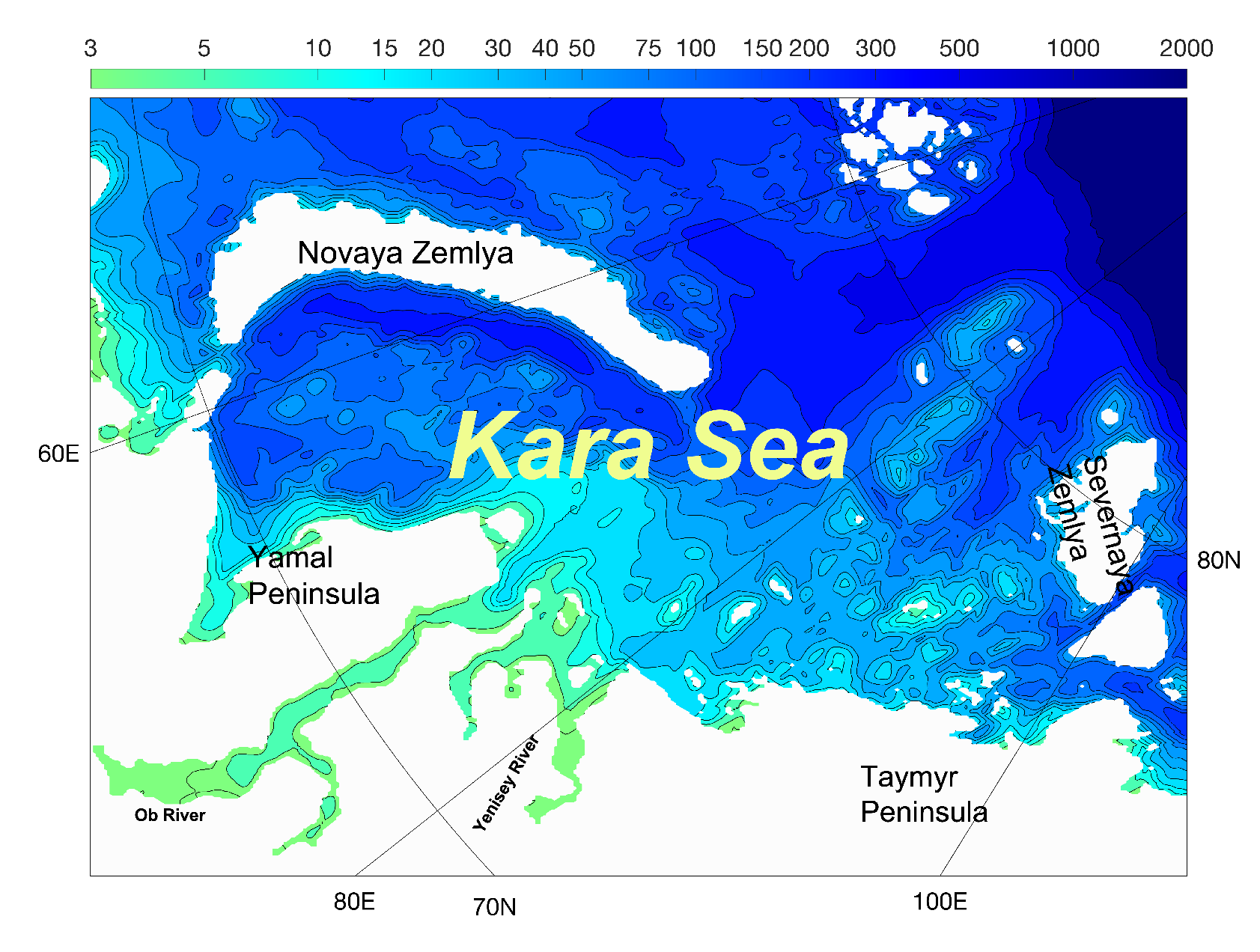
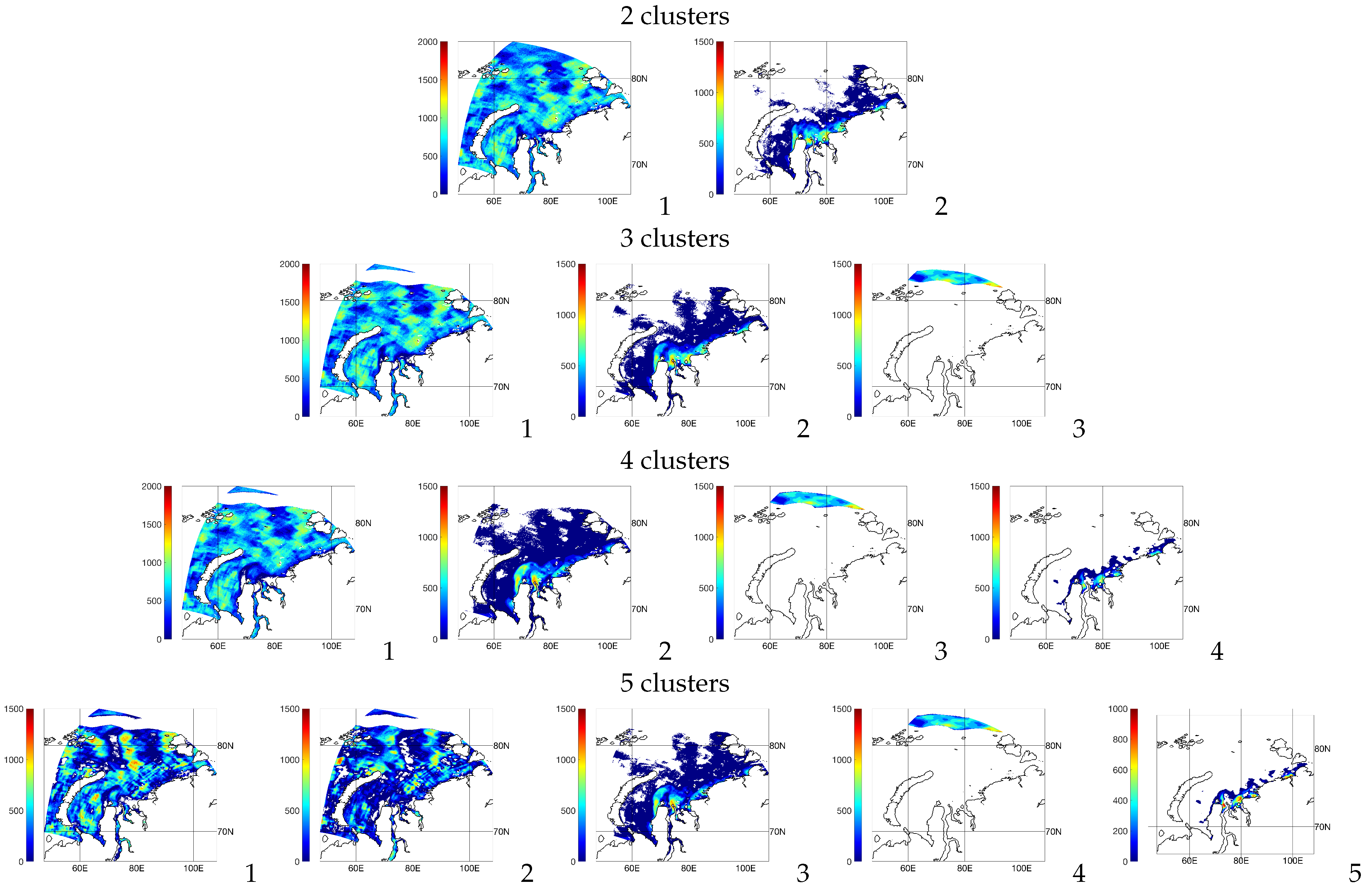
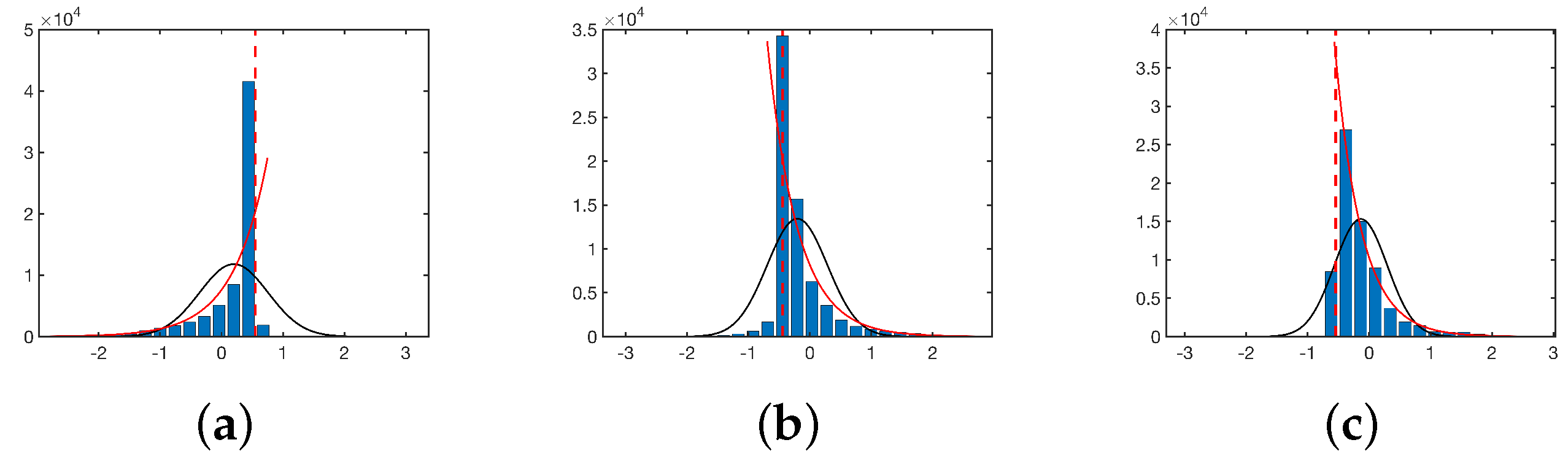
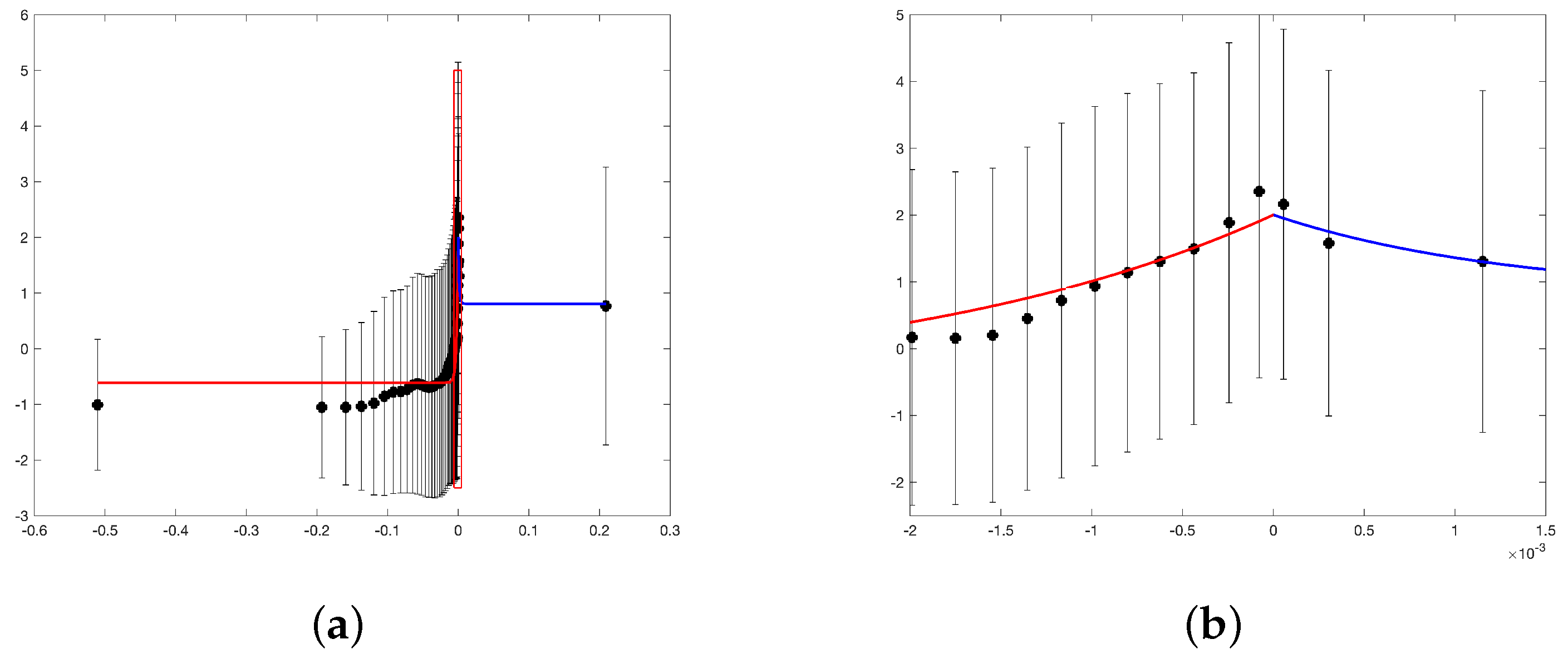
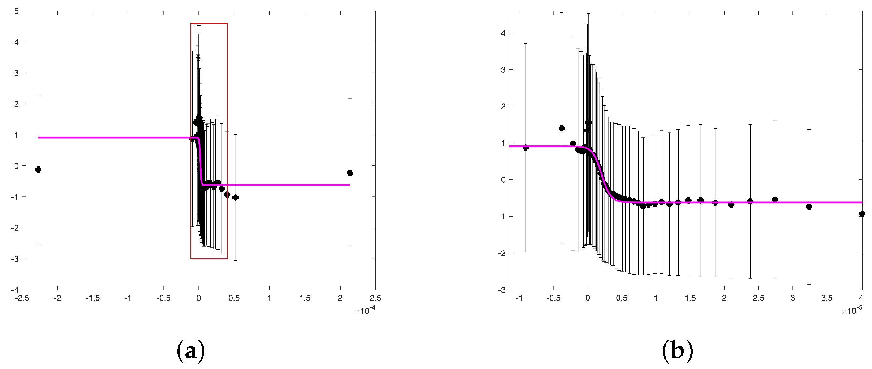
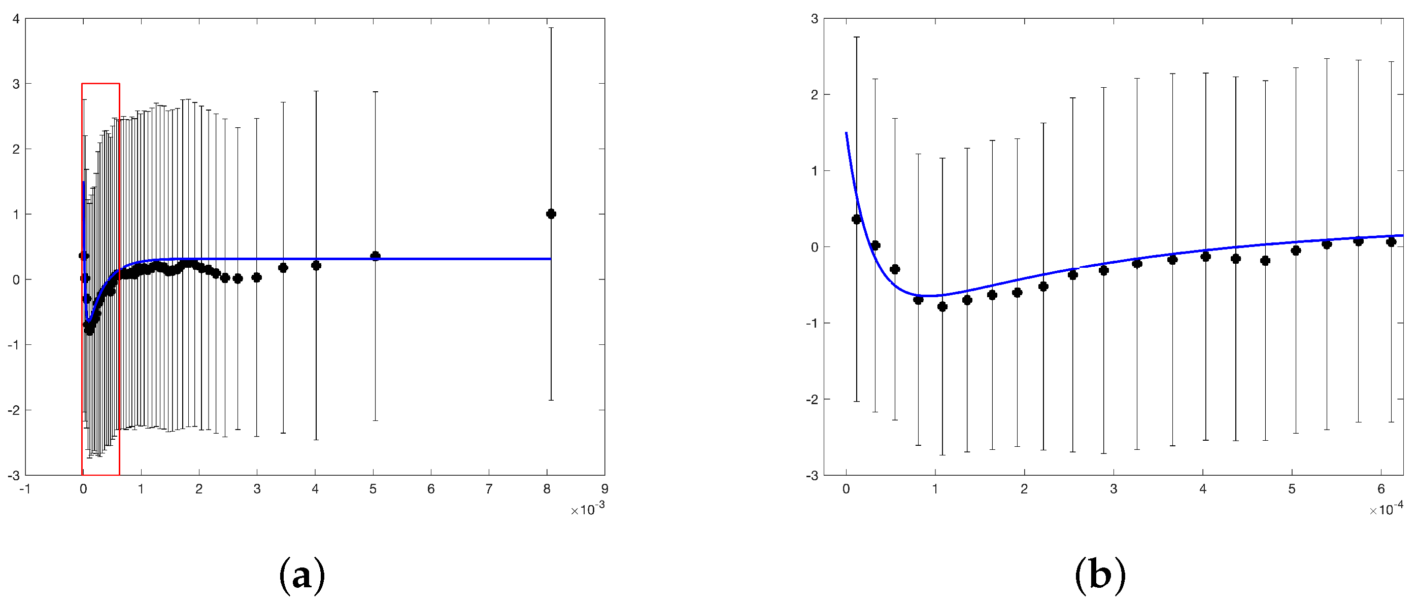
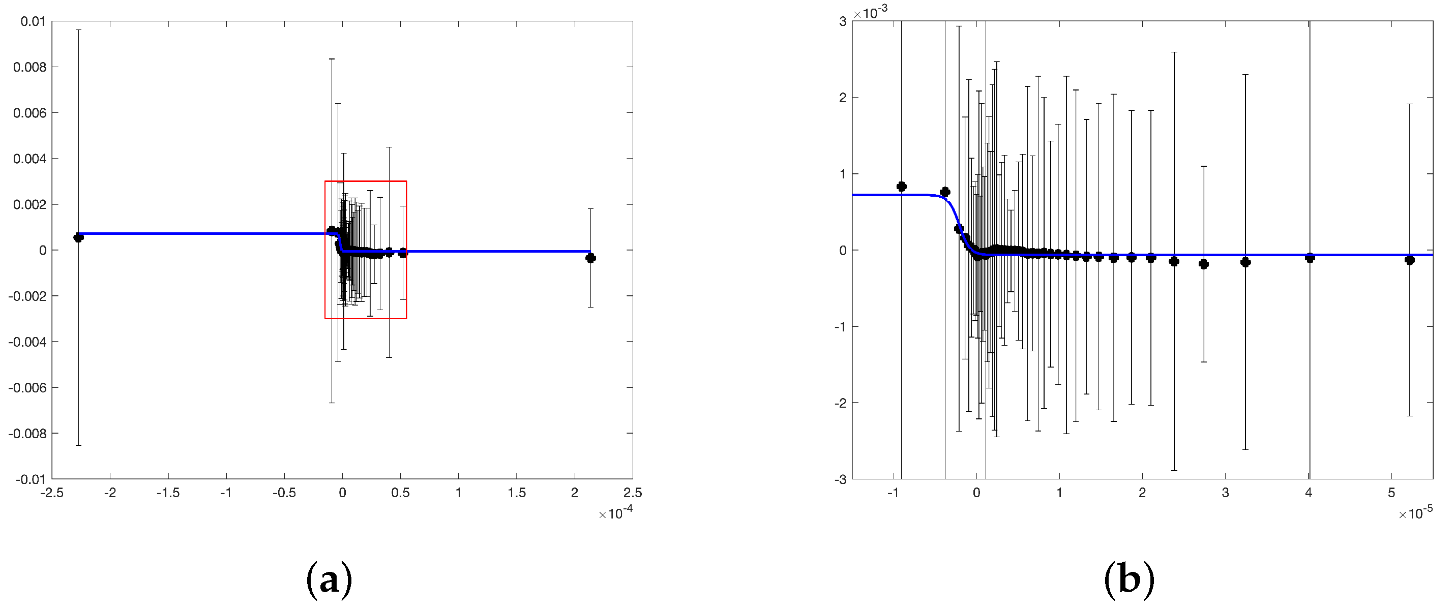
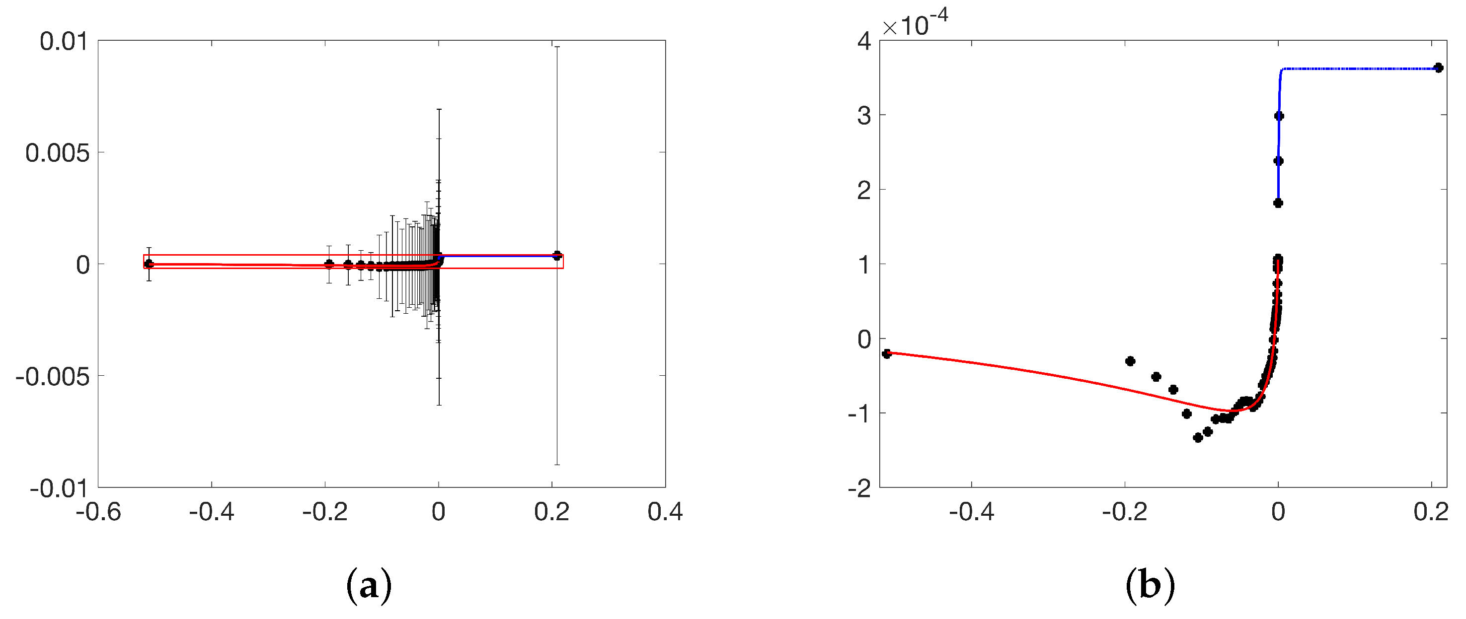
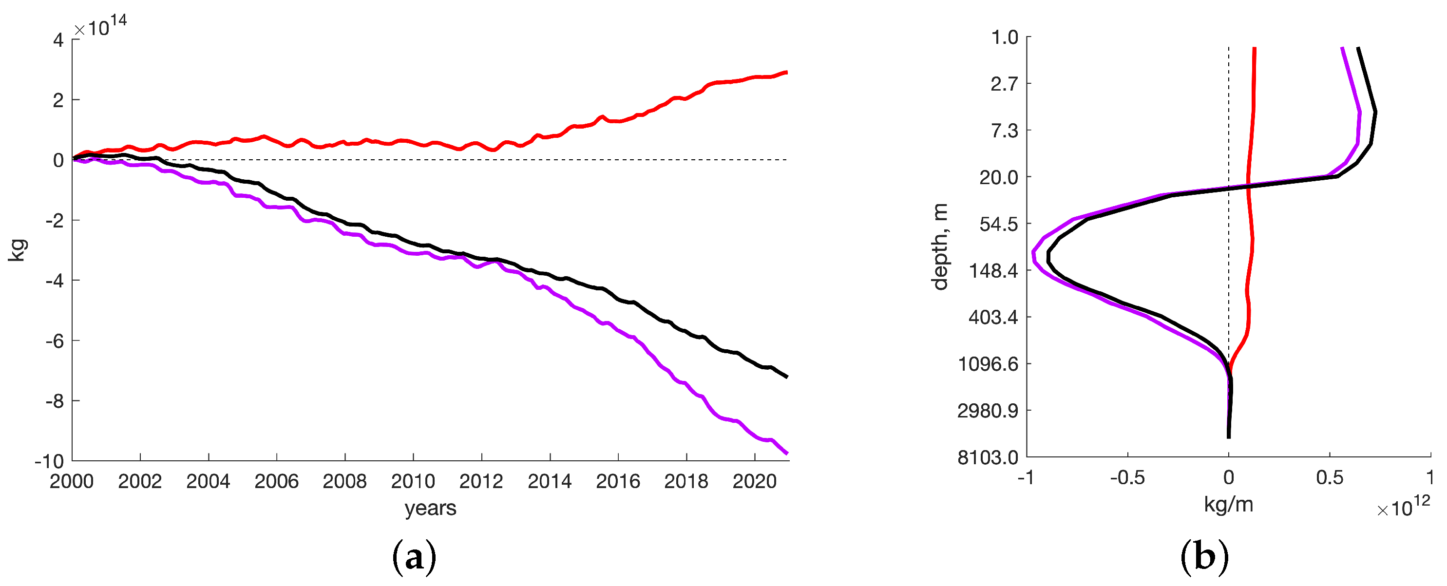
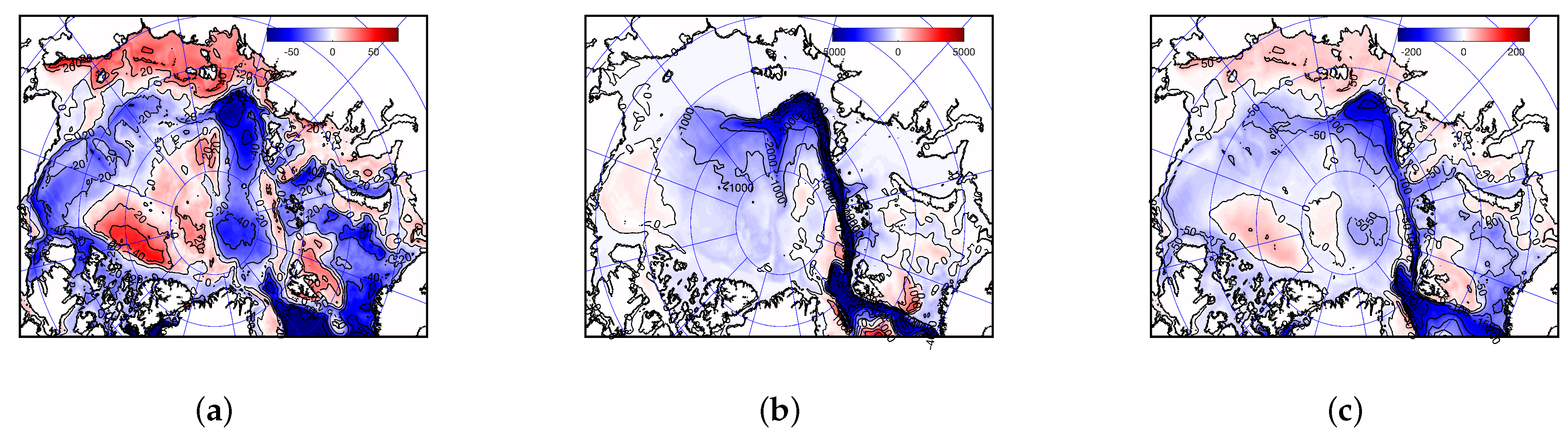
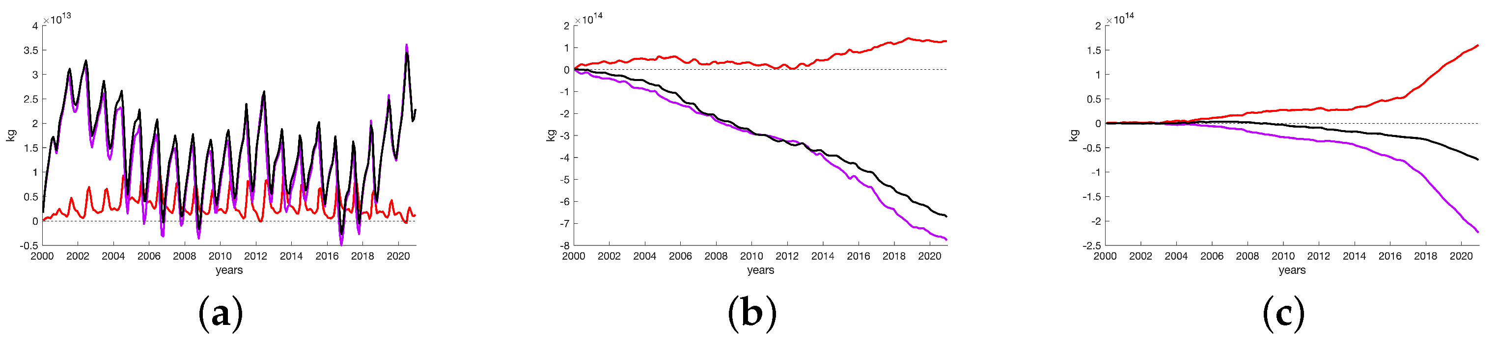
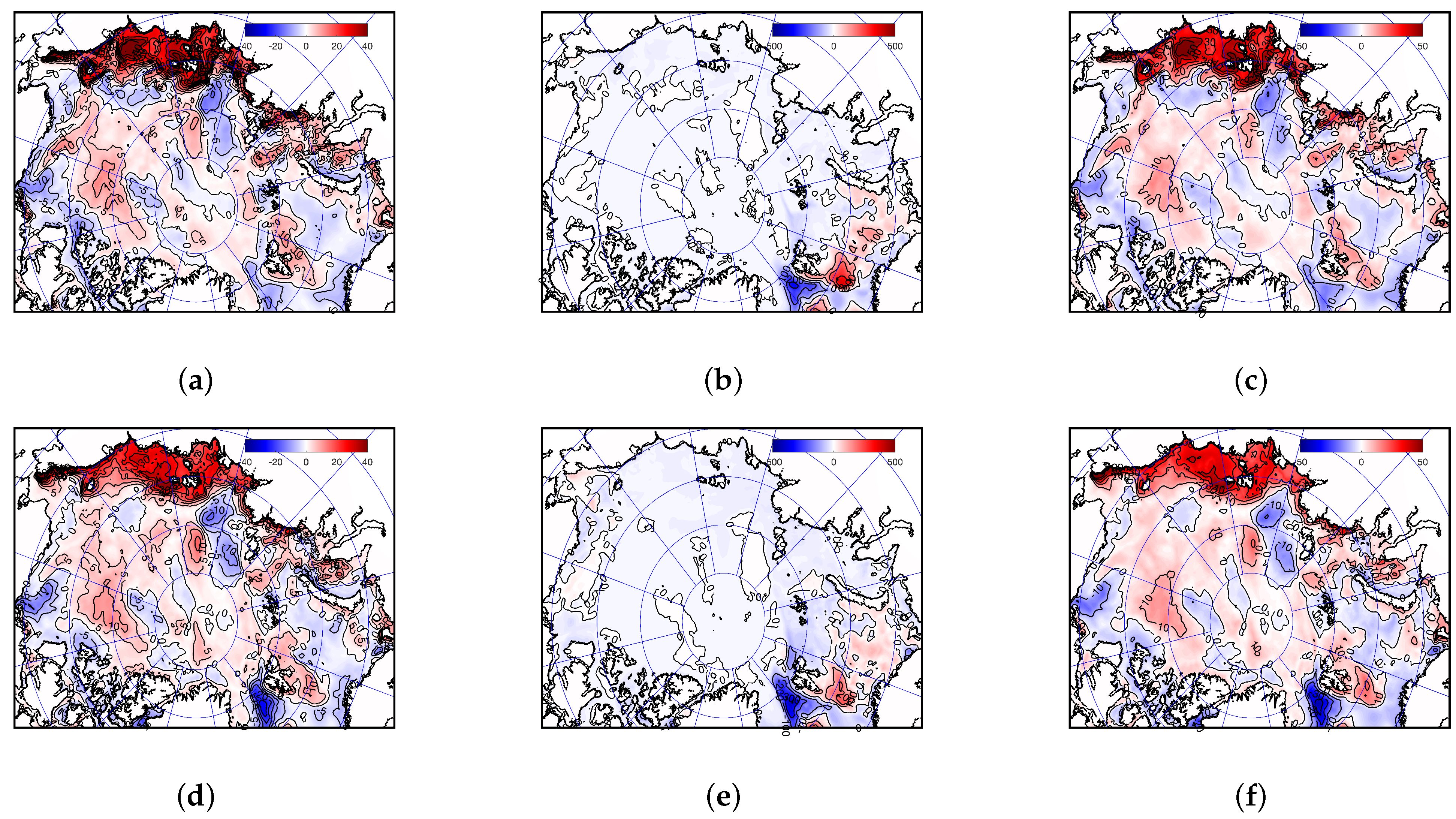
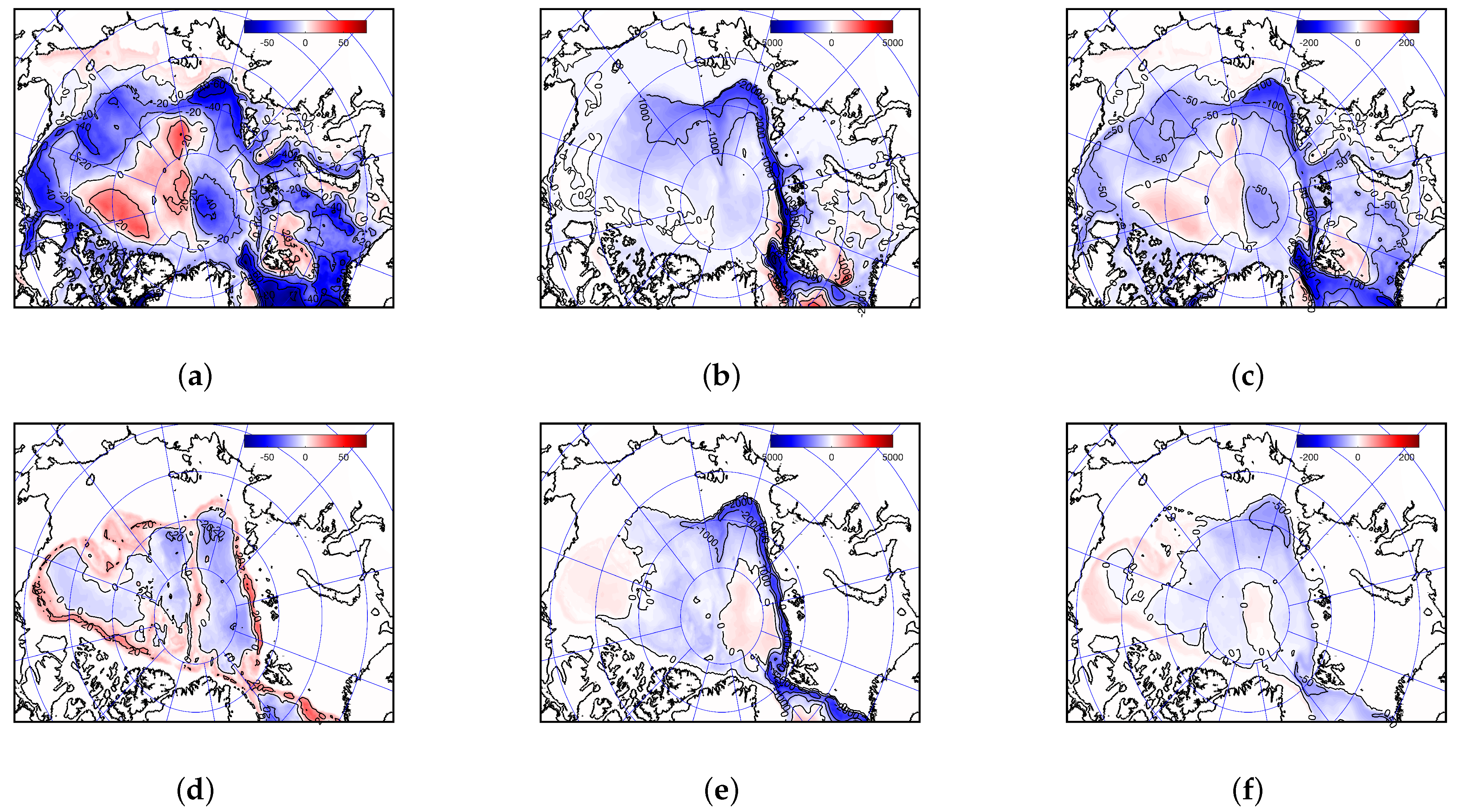
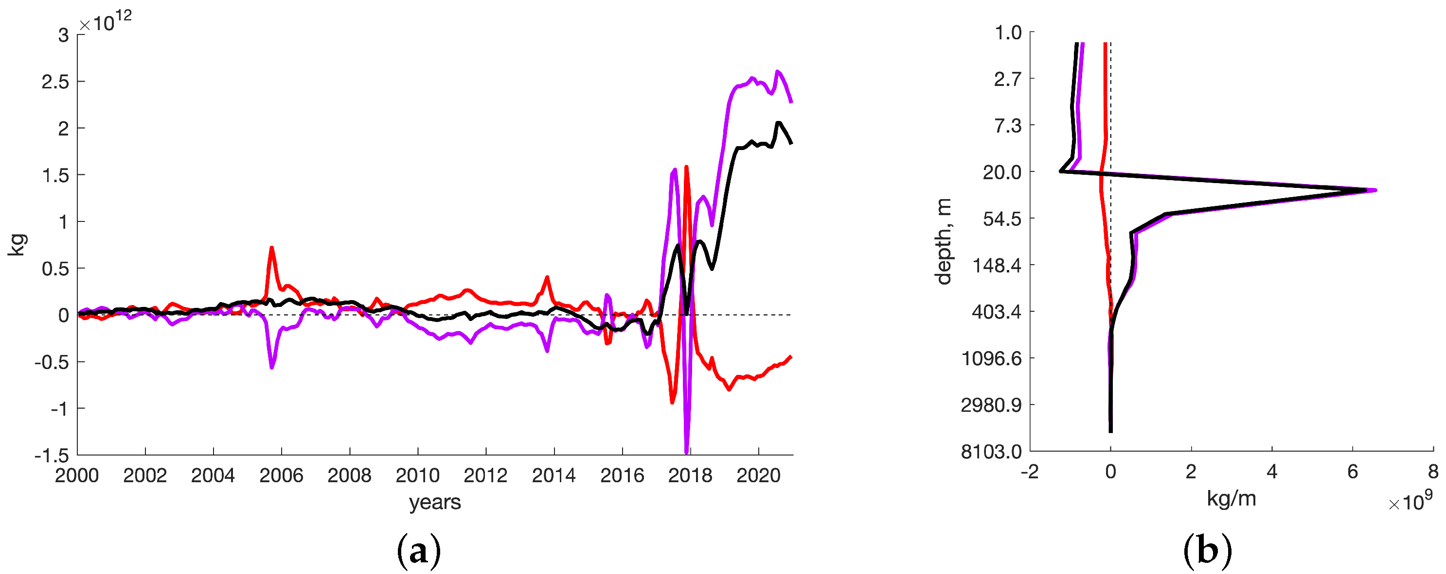
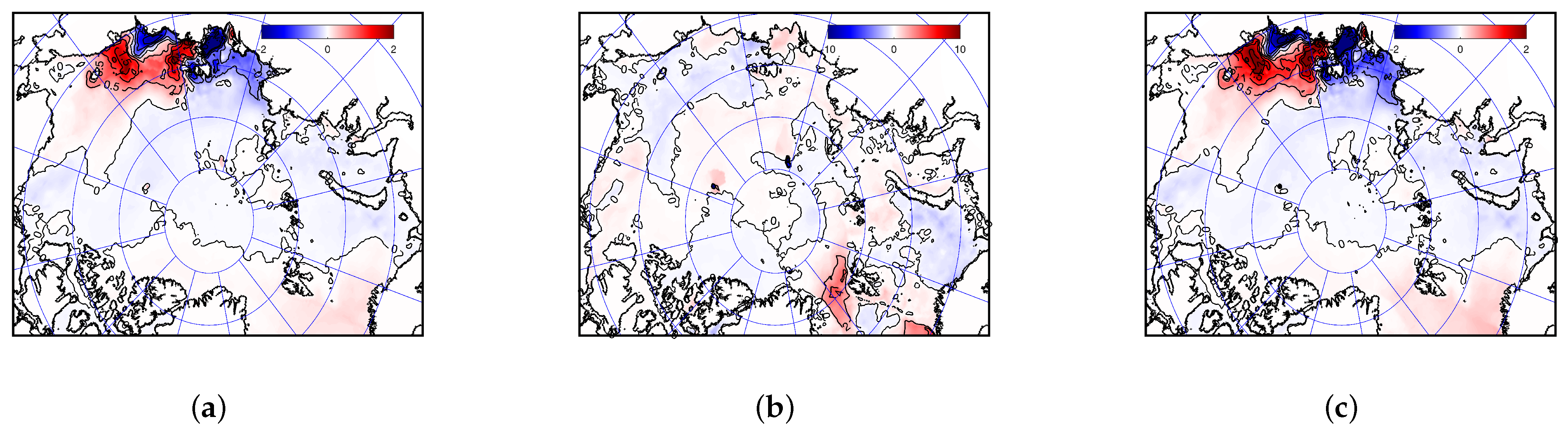
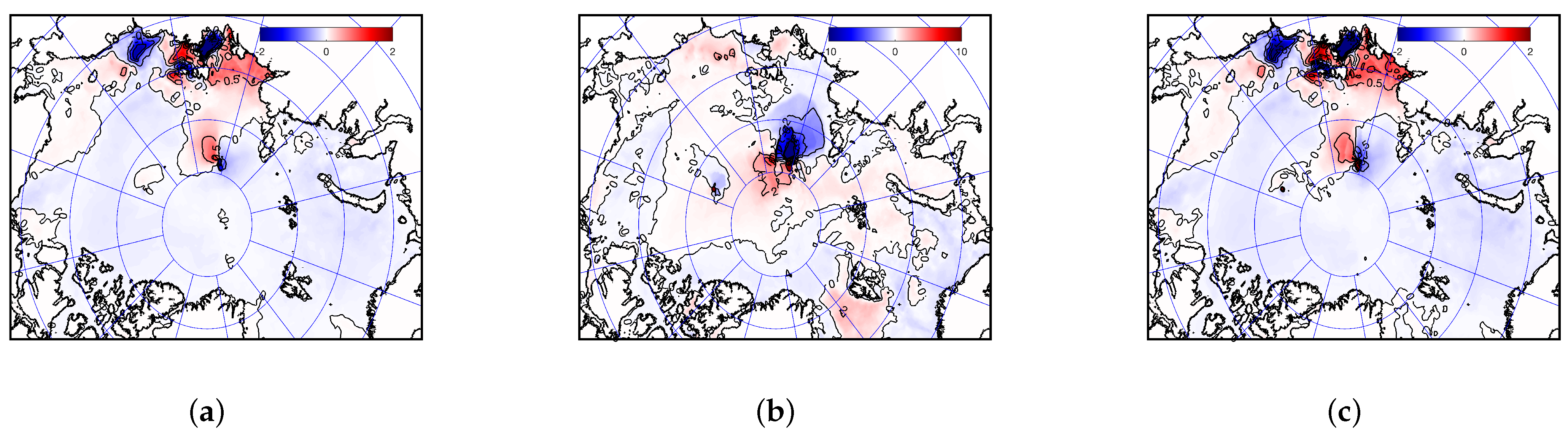
Table 1.
Geographic and physical large-scale characteristics, used for analysis of eddy mass transport dependencies. Here is the direction of the slope, and is the direction along the isobath. The first seven characteristics are selected after their dependency check.
Table 1.
Geographic and physical large-scale characteristics, used for analysis of eddy mass transport dependencies. Here is the direction of the slope, and is the direction along the isobath. The first seven characteristics are selected after their dependency check.
| No. | Symbolic Notation | Description |
|---|---|---|
| 1 | s | The value of the bottom slope |
| 2 | Component of the bottom density gradient in the direction of the slope | |
| 3 | Component of the density gradient in the direction along the isobath | |
| 4 | Shift of the velocity component U in the direction of the isobath | |
| 5 | Shift of the velocity component V in the direction of the slope | |
| 6 | Divergence of the velocity component V in the direction of the isobath | |
| 7 | Vertical component of the density gradient | |
| 8 | H | Ocean depth |
| 9 | z | Local (in situ) depth |
| 10 | Component of the density gradient in the direction of the bottom slope | |
| 11 | Component of the bottom density gradient in the direction along the isobath | |
| 12 | U | Flow velocity component in the direction of the slope |
| 13 | V | Flow velocity component in the direction along the isobath |
| 14 | Divergence of the velocity component U in the direction of the slope | |
| 15 | Geographic latitude | |
| 16 | Geographic longitude |
Table 2.
The results of sample clustering of the selected large-scale parameters into sets of from 2 to 5 clusters. Cluster percentage represents the percentage of elements in each cluster relative to the sample volume. DB, D, , and are the Davies–Bouldin index [37], Dunn index [38], clustering silhouette coefficient [39], and silhouette coefficient for each cluster [40], respectively (see description in Appendix A.1, Appendix A.2 and Appendix A.3). A, B, and C letters specify selected clusters referenced in text.
| Number of Clusters | No. | Cluster Percentage | DB | D | % | % |
|---|---|---|---|---|---|---|
| 2 | 1 | 91 | 1.62 | 0.953 | 78 | 95 |
| 2 | 9 | −89 | ||||
| 3 | 1 (A) | 88 | 1.37 | 0.958 | 74 | 96 |
| 2 (B) | 9 | −90 | ||||
| 3 (C) | 3 | −94 | ||||
| 4 | 1 | 81 | 1.70 | 0.526 | 57 | 91 |
| 2 | 13 | −84 | ||||
| 3 | 3 | −93 | ||||
| 4 | 3 | −95 | ||||
| 5 | 1 | 51 | 1.73 | 0.376 | 3 | 46 |
| 2 | 35 | −22 | ||||
| 3 | 9 | −81 | ||||
| 4 | 3 | −89 | ||||
| 5 | 3 | −93 |
Disclaimer/Publisher’s Note: The statements, opinions and data contained in all publications are solely those of the individual author(s) and contributor(s) and not of MDPI and/or the editor(s). MDPI and/or the editor(s) disclaim responsibility for any injury to people or property resulting from any ideas, methods, instructions or products referred to in the content. |
© 2023 by the authors. Licensee MDPI, Basel, Switzerland. This article is an open access article distributed under the terms and conditions of the Creative Commons Attribution (CC BY) license (https://creativecommons.org/licenses/by/4.0/).
Share and Cite
MDPI and ACS Style
Platov, G.; Iakshina, D.; Golubeva, E. Parametrization of Eddy Mass Transport in the Arctic Seas Based on the Sensitivity Analysis of Large-Scale Flows. Water 2023, 15, 472. https://doi.org/10.3390/w15030472
AMA Style
Platov G, Iakshina D, Golubeva E. Parametrization of Eddy Mass Transport in the Arctic Seas Based on the Sensitivity Analysis of Large-Scale Flows. Water. 2023; 15(3):472. https://doi.org/10.3390/w15030472
Chicago/Turabian StylePlatov, Gennady, Dina Iakshina, and Elena Golubeva. 2023. "Parametrization of Eddy Mass Transport in the Arctic Seas Based on the Sensitivity Analysis of Large-Scale Flows" Water 15, no. 3: 472. https://doi.org/10.3390/w15030472
Note that from the first issue of 2016, this journal uses article numbers instead of page numbers. See further details here.