


A Three-Parameter Hydrological Model for Monthly Runoff Simulation—A Case Study of Upper Hanjiang River Basin
1
School of Civil and Hydraulic Engineering, Huazhong University of Science and Technology, Wuhan 430074, China
2
Hubei Key Laboratory of Digital River Basin Science and Technology, Huazhong University of Science and Technology, Wuhan 430074, China
3
Bureau of Hydrology, Changjiang Water Resource Commission of the Ministry of Water Resource, Wuhan 430010, China
*
Author to whom correspondence should be addressed.
Water 2023, 15(3), 474; https://doi.org/10.3390/w15030474
Submission received: 3 December 2022
/
Revised: 13 January 2023
/
Accepted: 18 January 2023
/
Published: 25 January 2023
(This article belongs to the Topic Basin Analysis and Modelling)
Abstract
:Monthly hydrological models are useful tools for runoff simulation and prediction. This study proposes a three-parameter monthly hydrological model based on the proportionality hypothesis (TMPH) and applies to the Upper Hanjiang River Basin (UHRB) in China. Two major modules are involved in the TMPH: the actual evapotranspiration and runoff, in which the coupled water–energy balance equation and the proportionality hypothesis are used for calculation, respectively. It is worth mentioning that the proportionality hypothesis was extended to the partitioning of the available water into water loss and runoff at the monthly scale, which demonstrates that the ratio of runoff to its potential value is equal to the ratio of continuing water loss to its potential value. Results demonstrate that the TMPH model performs well when the NSE values are 0.79 and 0.83, and the KGE values are 0.86 and 0.78 for calibration period and validation period, respectively. The widely used two-parameter monthly water balance (TWBM) model and ABCD model are compared with the proposed model. Results show that TMPH performs better than TWBM model with NSE increased by 0.07 and 0.11, and KGE increased by 0.02 and 0.16, respectively, whereas the TMPH performs similarly as the ABCD model in the calibration period, and performs slightly better in the validation period, with NSE increased by 0.02, and KGE increased by 0.03. Sensitivity analysis show that the simulation result is most sensitive to parameter n, followed by SC and . In summary, the proposed model has strong applicability to the study area.
1. Introduction
Monthly hydrological models are useful tools for runoff simulation and prediction, which have been an active subject for decades. Because of their simple structure, low input requirement, and well simulation performance [1], monthly hydrological models have broad applications in water resource management, especially the monthly runoff simulation [2,3], assessment of climatic change impacts [4,5], as well as regional water resources assessments [6,7]. In general, the monthly hydrological models conceptualize hydrological processes using mathematical or physical formulas through two to five model parameters, and the water balance equation is regarded as the basis of many hydrological models.
The first monthly water balance model was originally presented by Thornthwaite [8] in the 1940s, and then it was subsequently revised by Thornthwaite and Mather [9]. Since then, numerous monthly hydrological models were proposed to meet various research purposes and different regions. Thomas [10] proposed a monthly water balance model named “abcd” model with four parameters, that is widely used in hydrological simulation research. In 1995, Boughton [11] developed the Australian water balance model, generally shortened to “AWBM” model. Xiong and Guo [12] presented a monthly water balance model with only two parameters (TWBM) in 1999, which has been one of the most widely used models in rainfall-runoff simulation because it achieves high simulation accuracy with a few parameters. Based on the TWBM, many new models have been developed, such as the DWBM model [13] and the TSPM model [3]. After nearly 70 years of development, various hydrological models have been proposed, even so, it is still meaningful to explore new hydrological models and their potential in practice.
To investigate the differences in model structure and application among different types of monthly hydrological models, many researchers have concentrated on the comparisons with those models [1,14,15]. For instance, Vandewiele and Ni Lar [16] applied two monthly models to 55 basins in 10 countries, and they concluded that no universal model can perform well for all watersheds; Cheng et al. [1] introduced five widely used monthly water balance models and then compared them in 443 Australian catchments, and they highlighted that monthly models with nonlinear baseflow modeling structure perform better in simulation. Previous studies have revealed that the major differences among the different monthly hydrological models focus on the solution of actual evaporation and runoff [13,15]. It also is found that the model becomes more and more complex with the number of parameters increasing due to a deeper understanding of the physical mechanism of hydrological processes. However, it is worth noting that the simple models are still effective and efficient, and even achieve better performance compared with the complex models in some simulations [14,17]. In the author’s opinion, the development of hydrological models should not always pursue complexity, and how to balance the model performance and complexity is the key issue.
However, hydrological processes are extremely complex in practice, including all hydrological components and the interactions, ties, and consequences among these components [18]. Lumped conceptual hydrological models always try to simplify complex hydrological processes, which can yield adequate results by greatly reducing the complexity of structure and input requirements. One of the most commonly used methods is the Soil Conservation Service (SCS) curve number model applied for a given rainfall event [19,20]. Poncea and Shetty [21] subsequently derived the generalized proportionality hypothesis as a more general form of the SCS method. Inspiring research by Wang and Tang [22] found that the generalized proportionality hypothesis can be identified as the commonality among hydrological models at different time scales and further study shows that the generalized proportionality hypothesis actually can serve as the result of the maximum entropy production principle [23,24]. In theory, the proportionality hypothesis offers a hydrological principle that the ratios of different hydrological variables to their potential values should be equal, which can be seen as a marker of coevolution in natural ecosystems [22,23,24]. In the previous work, the proportionality hypothesis has been successfully used for runoff simulation at the inter-annual [21,25], mean annual [22], and seasonal time scale [26]. In this study, we try a different partitioning of available water into two-component competition based on the proportionality hypothesis and seek if it can be used for the construction of a monthly water balance model and obtain promising simulation results.
In order to search the possibility of constructing the new hydrological models, and further search for a balance between the model performance and complexity. A three-parameter monthly model based on the proportionality hypothesis (denoted as TMPH) is developed in this study and then applied to Upper Hanjiang River Basin in China. The paper is organized as follows: In Section 2, the model structure is described in detail. Section 3 illustrates the study area and data source. Section 4 is devoted to results and discussion. At last, in Section 5, the conclusions are summarized.
2. Methodology
2.1. SCS Runoff Model and Generalized Proportionality Hypothesis
The SCS model has been widely used in runoff simulation at the event scale. In the SCS runoff model, water loss caused by vegetation interception and infiltration is assumed to be initial abstraction (), and this portion of the water does not compete with runoff. Thus, the remaining precipitation () is partitioned into two components, direct runoff () and continuing abstraction (), where the potential value for is the , and the potential value for is that defined as a variable related to soil properties. The competition between direct runoff and continuing abstraction can be explained by the proportionality hypothesis as follows (Equation (1)):
In the previous studies, Poncea and Shetty [21] have proposed the generalized proportionality hypothesis as a more general form of the SCS method. The available water () is partitioned into and . The can be deemed to be bounded by its potential value , and it should be preferred to meet , which doesn’t compete with . Furthermore, the potential for is the remaining available water . Thus, the partitioning can be determined by the generalized proportionality hypothesis as follows (Equation (2)):
Recently, Wang and Tang [22] have successfully applied the generalized proportionality hypothesis to the partitioning of precipitation into evaporation and runoff at the annual scale, in which the change of water storage in soil is neglected. In this case, the proportionality hypothesis demonstrates that the ratio of runoff to its potential value and the ratio of continuing evaporation to its potential value should be equal.
2.2. Proportionality Hypothesis Application for Monthly Water Balance
At the annual scale, the change of water storage in soil is usually neglected. However, for the monthly water balance, this change should be considered. In this case, the total available water can be defined as , which is the summation of precipitation () and water soil content at the beginning of the period (). The total available water can be partitioned into three components, direct runoff (), evaporation (), and soil water content at the end of the time t (). Here, we define the sum of and as water loss () to stand for the total water loss except for runoff in the basin during the period. Compared with the partitioning of precipitation into evaporation and runoff at an annual scale, we try to incorporate the change of soil water content in the division of water quantity. In fact, this partition can be seen as another form of the water balance equation (Equation (3)):
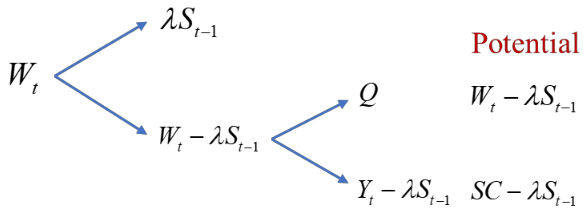
In the first stage, the available water is partitioned into two components, initial water loss and runoff potential, where the initial water loss includes initial evaporation and initial infiltration that are considered to be related to soil water content at the beginning of the period. At the second stage of the partitioning, the runoff potential is further subdivided into runoff and continuing water loss (i.e., continuing evaporation and continuing infiltration). The conceptual model of the partitioning is presented in Figure 1. A portion of water is lost without any competition with runoff by initial evaporation and initial infiltration, defined as the initial loss , and we consider as a percentage of (Equation (4)):
where represents the initial water loss ratio, that is, the first parameter in the study. The available water is preferred to meet the initial water loss, which does not compete with runoff. After that, the remaining available water () is then partitioned into runoff and continuing water loss (i.e., continuing evaporation and continuing infiltration). The sum of the and is the total water loss , which is constrained by its potential value . The relationship between runoff and continuing water loss is competitive, where the runoff is constrained by remaining available water, and the continuing water loss can be deemed to be bounded by the rest of its potential value (). Based on the proportionality hypothesis, we obtain (Equation (5)):
where represents the runoff; stands for the total available water; donates for the total water loss; is the initial water loss; and is a parameter representing the water loss capacity of the basin. The equation can be expressed as the ratio of continuing water loss to its potential value is equal to the ratio of runoff to its potential value.
2.3. Model Structure and Solution Method
2.3.1. The Solution of Actual Evapotranspiration
To estimate the actual evapotranspiration, the widely used coupled water–energy balance equation [27] is applied in this study. Following the Budyko hypothesis, the coupled water–energy balance equation was proposed for arbitrary time scales and has considered the effect of soil moisture content [28]. Moreover, the formula has obtained good results in numerous actual evaporation simulations at arbitrary time scales, and it has been widely used in region evaporation simulations [29], the establishment of a unified framework for water balance models [30], as well as climate and quantifying human impacts [31]. The equation can be described as follows (Equation (6)):
where (mm) and (mm) represent the actual evapotranspiration and the potential evapotranspiration, respectively; (mm) is the precipitation; (mm) is the water storage in the soil at the beginning of the time t; n is the third parameter in this study representing the characteristic of catchment underlying surface.
2.3.2. The Solution of Soil Water Content and Runoff
The calculation of soil water content (mm) can be obtained using the monthly proportion hypothesis and water balance equation. Based on Equation (3), the runoff (m3/s) can be calculated by (Equation (7)):
Thus, the monthly proportionality hypothesis can be described as follows (Equation (8)):
Expanding further we have (Equation (9)):
Then, (mm) can be obtained through , and (m3/s) is finally calculated by the water balance equation after the calculation of (mm) as follows (Equation (10)):
where represents the change of the water storage in soil, which is given as (Equation (11)):
where (mm) and (mm) mean the water storage in soil at the beginning of the time t and the water storage in soil at the end of the time t, respectively.
2.4. Parameter Optimization
A total of three parameters need to be calibrated in this study, namely initial water loss ratio (dimensionless), water loss capacity of the basin SC (mm), and the evapotranspiration parameter n (dimensionless), respectively. The definition and ranges are shown in Table 1.
For the optimization of model parameters, it is a task to minimize the error between simulated runoff and observed runoff. Thus, the objective function is considered to maximize the Nash–Sutcliffe Efficiency (NSE), which will be introduced in Section 2.5. In order to search the optimal parameters, a high-performance algorithm called the Shuffled Complex Evolution algorithm (SCE-UA) [32] is used in this study. The SCE-UA algorithm is a global optimization method, which is effective and of great use in the rainfall–runoff model since it can effectively solve common problems such as nonlinearity, discontinuity, as well as multi-extremum [33]. Here, we only give a brief description of the SCE-UA, and more details can be found in Duan’s paper [34].
2.5. Model Evaluations
In this study, two widely used efficiency criteria are applied to evaluate the performance of the hydrological model, including Nash–Sutcliffe Efficiency [35] and Kling–Gupta Efficiency [36].
- (1)
- Nash-Sutcliffe Efficiency (NSE)
The NSE is the most widely used statistical criterion to evaluate the goodness-of-fit in runoff simulation. The value of NSE varies from to 1. In general, a value closer to 1 represents a better model performance. NSE can be calculated as follows (Equation (12)):
where and represent the simulated runoff and observed runoff at time , respectively; is the number of months for simulation, and is the mean of all observations. In general, model performance can be considered satisfactory if NSE > 0.50 [37].
- (2)
- Kling–Gupta Efficiency (KGE)
The KGE is also selected to justify the simulation performance that is sensitive to high flows and variance [38], with the value ranging from to 1. In general, the value of KGE close to 1 means good fitting effect. The KGE is composed of three basic assessments, including Pearson’s linear correlation coefficient (), the ratio of standard deviations of simulation and observation (), as well as the ratio of the average value of simulation and observation (), which can be calculated as follows (Equation (13)):
3. Case Study
3.1. Study Area
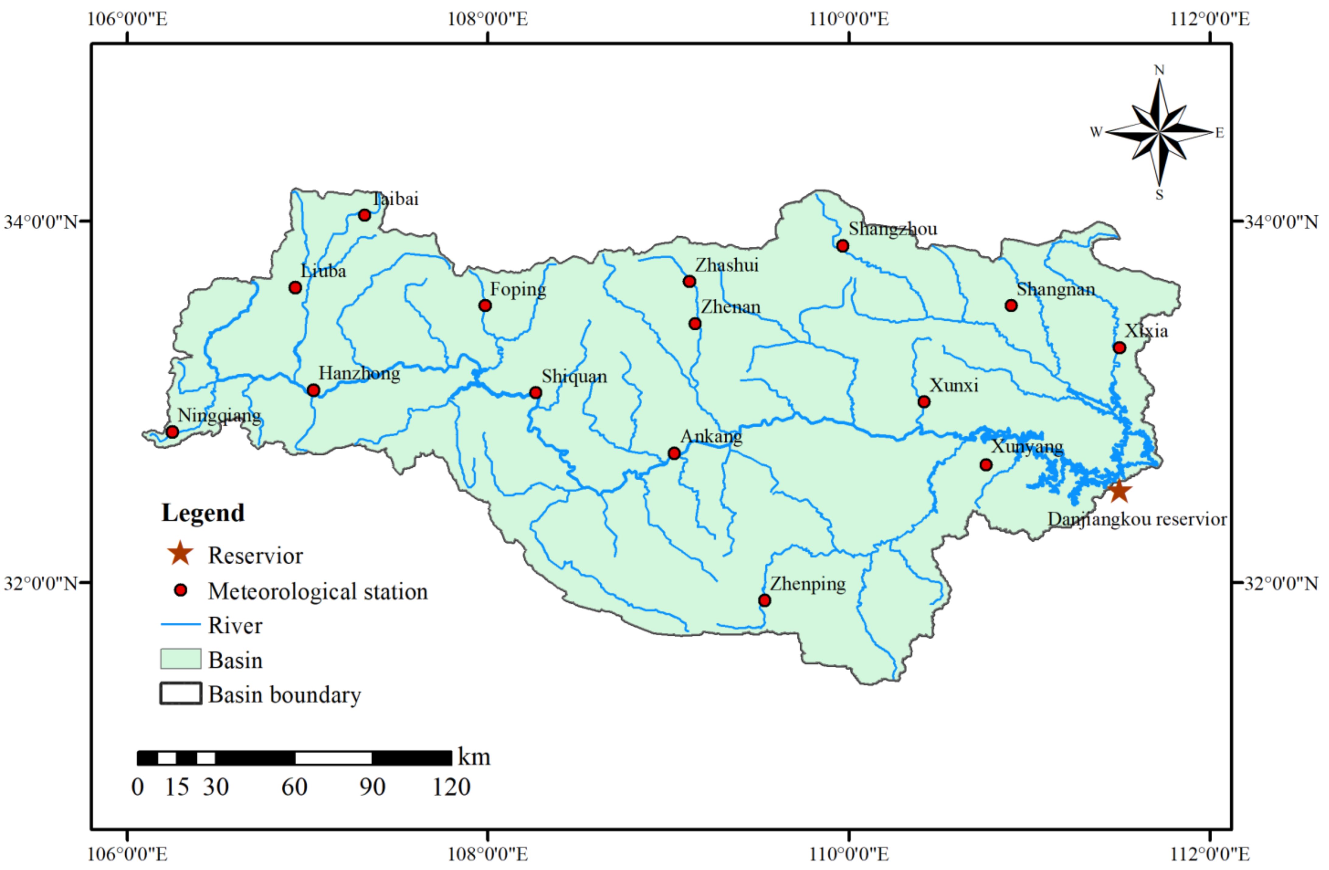
The Upper Hanjiang River Basin, with a catchment area of 95,217 km2, is located in the upper reaches of Hanjiang River Basin in China, accounting for 60% of the total Hangjiang river basin area. For simplicity, the Upper Hanjiang River Basin is referred to as UHRB, as shown in Figure 1. UHRB includes innumerous rivers and complex terrain with mostly mountainous valleys and small areas of plains. Affected by the subtropical monsoon climate, the mean annual temperature varies from 12 °C to 16 °C, and the mean annual precipitation is approximately 873 mm with nearly 80% of the annual precipitation occurring in the summer. The average annual runoff is 4.11 billion m3. Correspondingly, the runoff distribution is uneven throughout the year, which is similar to that of precipitation, with great inter-annual differences.
Danjiangkou Reservoir is the outlet of the UHRB basin, as one of the main water sources of the South-to-North Water Transfer Project. It plays an important role in stable water supply and effective operation. And it has comprehensive functions of power generation, water supply, flood control, irrigation, shipping, tourism, etc. Accurate monthly runoff prediction is fundamental for the Danjiangkou reservoir operation. Due to its crucial function, there is a great need to predict future runoff in the basin for reservoir operation and control.
3.2. Data Sources
Monthly evaporation data, monthly rainfall data, as well as monthly runoff data spanning the years 1987–2020 are used in this study, in which the first 20 years (1987–2006) are selected as the calibration period, and the rest of the 14 years (2007–2020) are selected as the validation period. In particular, the evaporation and rainfall data, measured at 15 hydrological stations are extracted from the National Meteorological Information Centre (http://data.cma.cn), accessed on 1 June 2021. The used evaporation and rainfall data is the mean of all observations of 15 stations in UHRB, and the distribution of the hydrological stations is shown in Figure 2. Furthermore, the used runoff data is obtained from Danjiangkou Reservoir station which is the outlet of the UHRB by reduction calculation.
4. Result and Discussion
4.1. Model Performance and Parameter Result
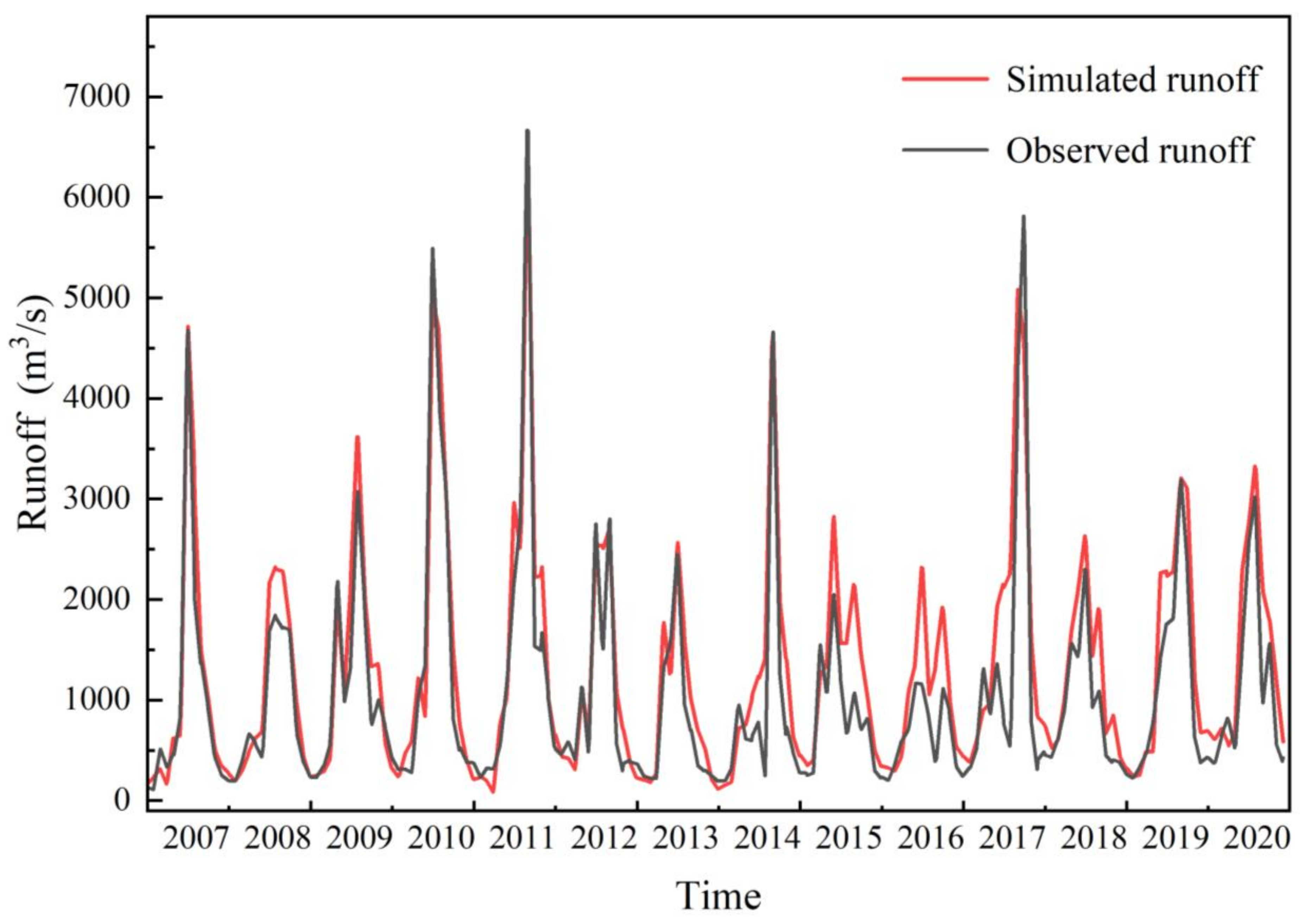
The proposed TMPH model has been applied to the selected basin of UHRB. Simulation results, including the optimization result of the parameters, the value of the evaluation indicators, are introduced below. To search the optimal parameters, the SCE-UA algorithm was used in this study, and the optimization result of the parameters was λ = 0.43, SC = 629.44, and n = 0.65. The values of NSE are 0.79 for the calibration period and 0.83 for the validation period. In general, the result is quite good. The KGE values are also calculated in the study, which are 0.86 for the calibration period and 0.78 for the validation period. Figure 3 shows the simulation in the validation period, and it is found that the simulation generally performs well. Overall, the results demonstrated that the proposed TMPH model can be successfully used for simulating and forecasting the monthly runoff effectively in UHRB and obtain quite good simulation accuracy.
4.2. Comparison of Model Performance with the TWBM Model and the ABCD Model
To better verify the simulation effect, we compare and analyze the proposed models in the selected basin. The TWBM model is one of the most widely used models in rainfall–runoff simulation because it achieves high simulation accuracy with few parameters. It has shown a good performance in runoff simulation and forecast in numerous studies [39,40]. Furthermore, the ABCD model has been widely used around the world. Thus, the TWBM model and ABCD model were selected as the base models for comparison with the proposed model. The formulas for ABCD model and TWBM model are given in the Appendix A. Table 2 shows the comparasion results of TMPH, TWBM, and ABCD.
Specifically, compared with the TWBM model, the TMPH model has improved the simulation accuracy in calibration period, when the value of NSE increased from 0.72 to 0.79, while simultaneously increasing the KGE from 0.84 to 0.86. A similar result was shown in the validation period, and the NSE improved from 0.72 to 0.83, with an increasing of KGE from 0.62 to 0.78. Compared with the ABCD model, the TMPH model has similar results in the calibration period, with NSE values of 0.79 and 0.80 for TMPH and ABCD, respectively. The KGE values are both 0.86. While in the validation period, the TMPH model improved slightly when the value of NSE increased from 0.81 to 0.83, while KGE increased from 0.75 to 0.78. Together these results indicated that TMPH achieves better simulation results than TWBM under the condition of adding only one more parameter, whereas the model accuracy of TMPH is comparable to that of ABCD.
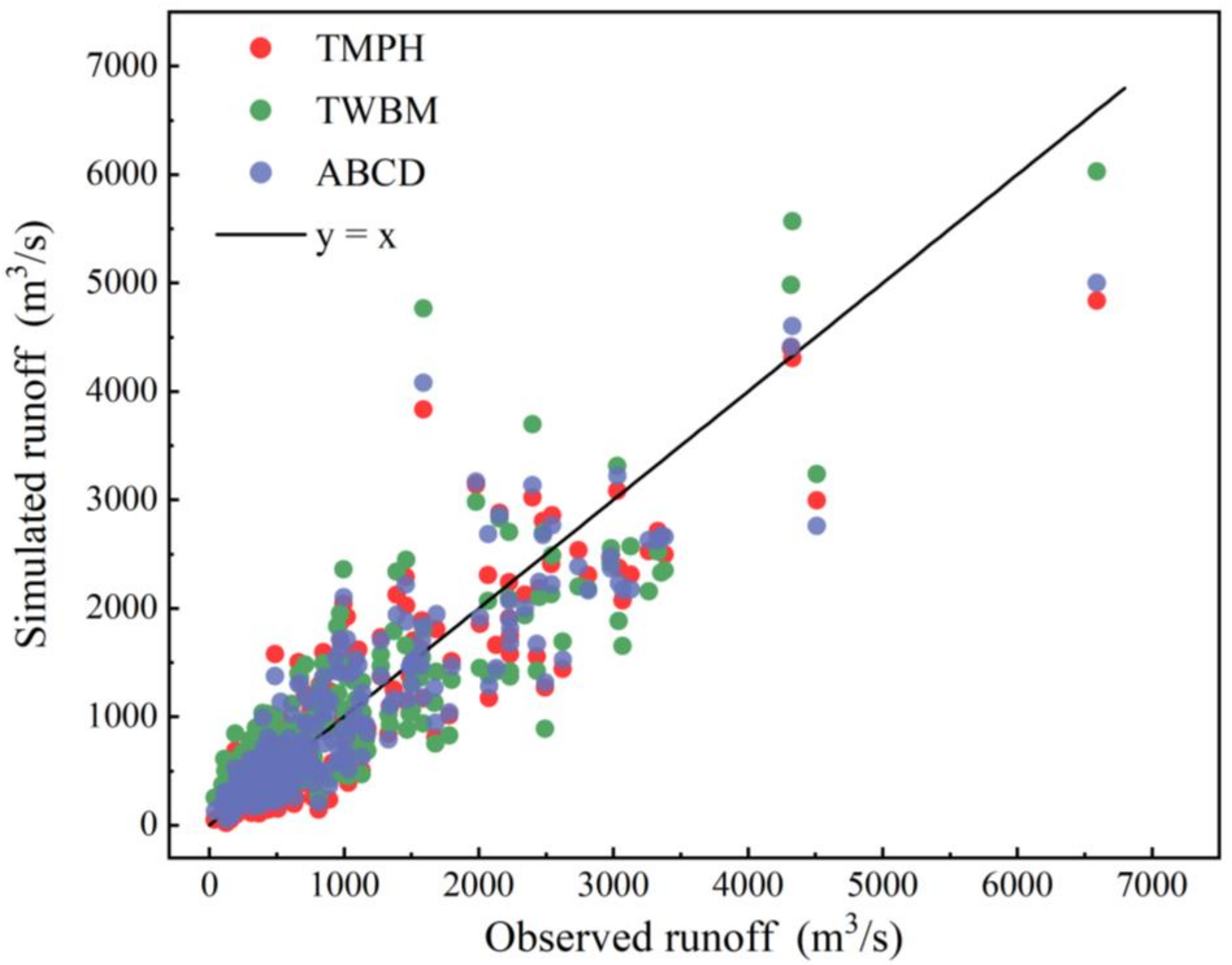
For a more clear demonstration of the performance difference among the three models, two figures, that is, Figure 4 and Figure 5, are plotted, which have shown the simulated runoff scatter diagram by TMPH, TWBM, and ABCD in the calibration period and validation period, respectively. In the calibration period, as shown in Figure 4, most of the points fall within a very close range of the fuction . By contrast, the TMPH model and ABCD model perform better at higher runoff values, especially when the runoff is more than 3000 m3/s, whereas at lower values the performance of the three models is almost the same. It becomes more apparent in Figure 5, where the points of TMPH are more concentrated, especially at higher runoff values.
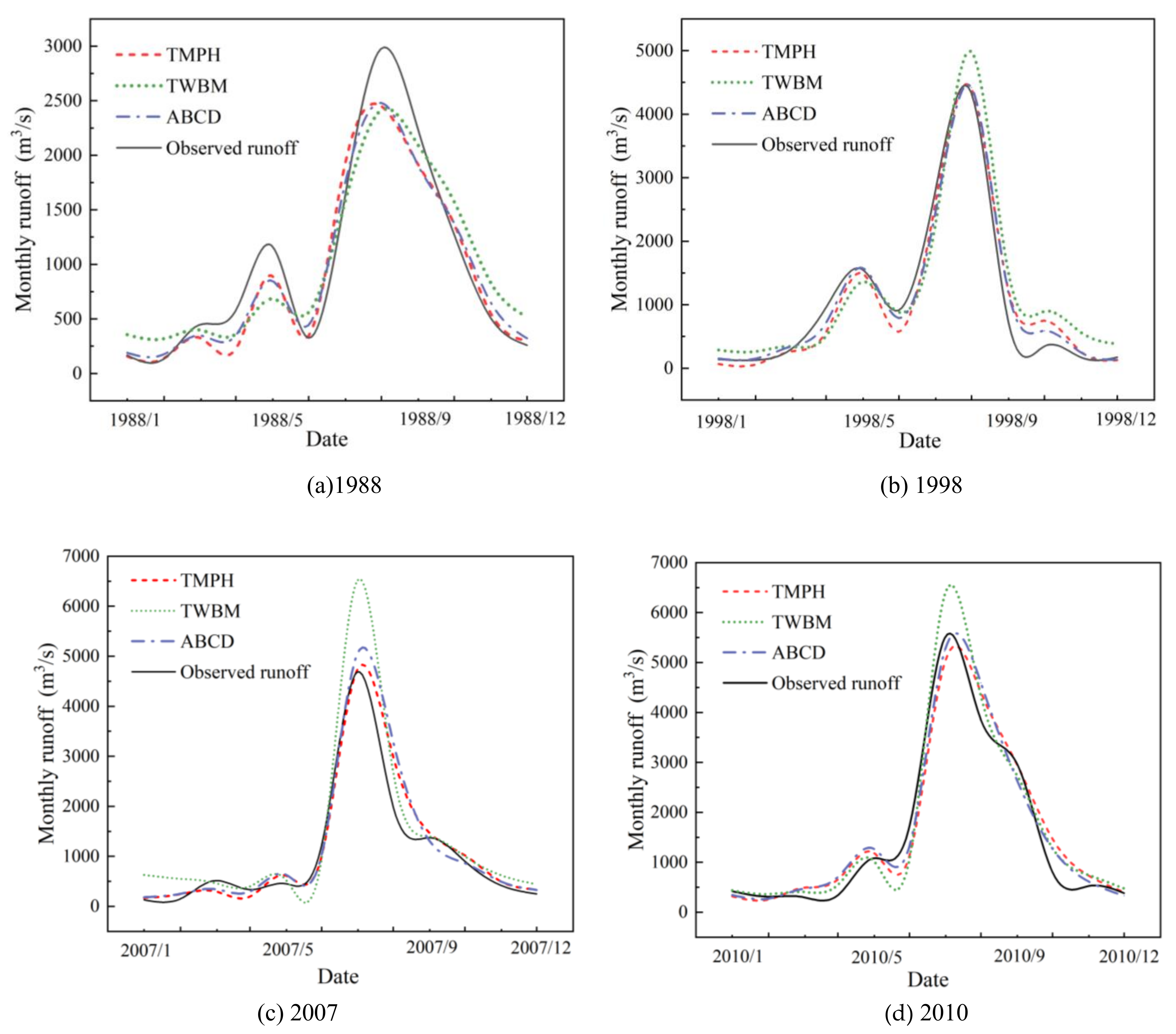
Moreover, Figure 5 presents the performance difference among TMPH, TWBM, and ABCD in the selected year, in which Figure 5a,b represent the years of 1988 and 1998 in the calibration period, respectively, and Figure 5c,d represents the years of 2007 and 2010 in the calibration period, respectively. It can be found that the peaks for maximum monthly runoff for both TMPH and ABCD are very close to the observed runoff, whereas the TMBM peak leads to an overestimation. The result indicated that the monthly runoff simulated by the proposed TMPH model was improved to some extent compared with the TWBM, and TMPH show a similar result with the ABCD model.
4.3. Sensitivity Analysis of TMPH Model Parameters
It is of great importance to study the sensitivities of model parameters to improve the efficiency and accuracy of model parameter calibration. This paper analyzes the response of two performance evaluation indexes of TMPH model, that is, NSE and KGE, to the changes of three parameters. The specific approach is to take the optimal result of automatic parameter calibration as the fixed value, and change each parameter by in turn, and observe the response of NSE and KGE. The results are shown in Table 3.
After changing each parameter by +50% and −50%, it can be found that for NSE, the change of parameter n has the greatest impact on it, with changes of −26.58% and −116.46%, followed by parameter SC with changes of −6.33% and −18.99%, and parameter with the minimum changes of −3.80% and −2.53%, respectively. While for KGE, the change of parameter n still has the greatest influence on it, with changes of −23.26% and −84.88%, the second one is parameter SC with changes of −19.77% and −17.44%, and the third is parameter with the smallest changes of −11.63% and 2.33%, respectively. In summary, the simulation result is most sensitive to parameter n, followed by parameter SC and parameter .
5. Conclusions
In this study, we developed a three-parameter monthly hydrological model based on the proportionality hypothesis, and successfully simulated the monthly runoff in the UHRB in China. In the TMPH model, the coupled water-energy balance equation is applied to estimate the actual evaporation, and the proportionality hypothesis is used for runoff calculation. Conclusions derived are as follows:
- (1)
- The proposed TMPH model shows good performance in the monthly runoff simulation in UHRB, with a simple model structure and few parameters. Specifically, the values of NSE are 0.79 for the calibration period and 0.83 for the validation period, with the value of KGE are 0.86 for the calibration period and 0.78 for the validation period;
- (2)
- In UHRB, the proposed TMPH model have better performance than the TWBM model, especially in the case of higher runoff values. Specifically, the value of NSE increases from 0.72 to 0.79 for the calibration period, and from 0.72 to 0.83 for the validation period. Meanwhile, the value of KGE increases from 0.84 to 0.86 for the calibration period, and from 0.62 to 0.78 for the validation period;
- (3)
- In UHRB, the TMPH model shows a comparable result with the ABCD model in the calibration period, with NSE values of TMPH and ABCD of 0.79 and 0.80, respectively, the KGE values are both 0.86, respectively. While in the validation period, the TMPH model has improved slightly, with the value of NSE increasing from 0.81 to 0.83, while increasing the KGE from 0.75 to 0.78;
- (4)
- The sensitivity analysis of TMPH model parameters shows that the simulation result is most sensitive to parameter n, followed by parameter SC and parameter .
It is worth noting that the proposed TMPH model mainly applied to humid and subhumid areas, while its performance in arid regions has not been verified. Future efforts will concentrate on the improvement of runoff modeling in arid regions.
Author Contributions
Conceptualization, B.Y. and Y.Z.; Data curation, B.F.; Investigation, J.Z. and Y.T.; Methodology, B.Y. and Y.Z.; Supervision, B.Y.; Validation, B.F., Y.Z. and J.Z.; Visualization, Y.T.; Writing—original draft, Y.Z. and B.Y.; Writing—review & editing, Y.Z. All authors have read and agreed to the published version of the manuscript.
Funding
This study is financially supported by the National Key R&D Program of China (2021YFC3200301), the National Natural Science Foundation of China (52079054), and the Natural Science Foundation of Hubei Province (2021CFB325).
Data Availability Statement
All data, models, and code that support the findings of this study are available from the corresponding author upon reasonable request.
Conflicts of Interest
The authors declare no conflict of interest.
Appendix A. Monthly Models
Appendix A.1. TWBM Model
Expanding further we have:
Appendix A.2. ABCD Model
The ABCD model is an efficient four-parameter conceptual hydrological model, which is described as follows [10].
References
- Cheng, S.; Cheng, L.; Liu, P.; Zhang, L.; Xu, C.; Xiong, L.; Xia, J. Evaluation of baseflow modelling structure in monthly water balance models using 443 Australian catchments. J. Hydrol. 2020, 591, 125572. [Google Scholar] [CrossRef]
- Schär, C.; Vasilina, L.; Pertziger, F.; Dirren, S. Seasonal runoff forecasting using precipitation from meteorological data assimilation systems. J. Hydrometeorol. 2004, 5, 959–973. [Google Scholar] [CrossRef]
- Deng, C.; Wang, W. A two-stage partitioning monthly model and assessment of its performance on runoff modeling. J. Hydrol. 2021, 592, 125829. [Google Scholar] [CrossRef]
- Mohseni, O.; Stefan, H.G. A monthly streamflow model. Water Resour. Res. 1998, 34, 1287–1298. [Google Scholar] [CrossRef]
- Wang, G.; Xia, J.; Chen, J. Quantification of effects of climate variations and human activities on runoff by a monthly water balance model: A case study of the Chaobai River basin in northern China. Water Resour. Res. 2009, 45, W00A1. [Google Scholar] [CrossRef] [Green Version]
- Zhang, Z.; Balay, J.W.; Liu, C. Regional regression models for estimating monthly streamflows. Sci. Total Environ. 2020, 706, 135729. [Google Scholar] [CrossRef] [PubMed]
- Ndzabandzaba, C.; Hughes, D.A. Regional water resources assessments using an uncertain modelling approach: The example of Swaziland. J. Hydrol. Reg. Stud. 2017, 10, 47–60. [Google Scholar] [CrossRef]
- Thornthwaite, C.W. An approach toward a rational classification of climate. Geogr. Rev. 1948, 38, 55–94. [Google Scholar] [CrossRef]
- Thornthwaite, C.W.; Mather, J.R. The Water Balance; Laboratory of Climatology, Drexel Institute of Technology: Centerton, NJ, USA, 1955; Volume 8, pp. 1–104. [Google Scholar]
- Thomas, H. Improved Methods for National Water Assessment: Final Report; U.S. Geological Survey: Reston, VA, USA, 1981; Volume 44.
- Boughton, W.C. An Australian water balance model for semiarid watersheds. J. Soil Water Conserv. 1995, 50, 454–457. [Google Scholar]
- Xiong, L.; Guo, S. A two-parameter monthly water balance model and its application. J. Hydrol. 1999, 216, 111–123. [Google Scholar] [CrossRef]
- Zhang, L.; Potter, N.; Hickel, K.; Zhang, Y.; Shao, Q. Water balance modeling over variable time scales based on the Budyko framework—Model development and testing. J. Hydrol. 2008, 360, 117–131. [Google Scholar] [CrossRef]
- Bai, P.; Liu, X.; Liang, K.; Liu, C. Comparison of performance of twelve monthly water balance models in different climatic catchments of China. J. Hydrol. 2015, 529, 1030–1040. [Google Scholar] [CrossRef]
- Jiang, T.; Chen, Y.Q.D.; Xu, C.Y.Y.; Chen, X.H.; Chen, X.; Singh, V.P. Comparison of hydrological impacts of climate change simulated by six hydrological models in the Dongjiang Basin, South China. J. Hydrol. 2007, 336, 316–333. [Google Scholar] [CrossRef]
- Vandewiele, G.L.; Ni Lar, W. Monthly water balance models for 55 basins in 10 countries. Hydrol. Sci. J. 1998, 43, 687–699. [Google Scholar] [CrossRef]
- Ye, W.; Bates, B.; Viney, N.; Sivapalan, M.; Jakeman, A. Performance of conceptual rainfall-runoff models in low-yielding ephemeral catchments. Water Resour. Res. 1997, 33, 153–166. [Google Scholar] [CrossRef]
- Al-Ghobari, H.; Dewidar, A.Z. Integrating GIS-Based MCDA Techniques and the SCS-CN Method for Identifying Potential Zones for Rainwater Harvesting in a Semi-Arid Area. Water 2021, 13, 704. [Google Scholar] [CrossRef]
- Amatya, D.M.; Walega, A.; Callahan, T.J.; Morrison, A.; Vulava, V.; Hitchcock, D.R.; Williams, T.M.; Epps, T. Storm event analysis of four forested catchments on the Atlantic coastal plain using a modified SCS-CN rainfall-runoff model. J. Hydrol. 2022, 608, 127772. [Google Scholar] [CrossRef]
- Kumar, A.; Kanga, S.; Taloor, A.K.; Singh, S.K.; Đurin, B. Surface runoff estimation of Sind river basin using integrated SCS-CN and GIS techniques. HydroResearch 2021, 4, 61–74. [Google Scholar] [CrossRef]
- Poncea, V.M.; Shetty, A.V. A conceptual model of catchment water balance: 1. Formulation and calibration. J. Hydrol. 1995, 173, 27–40. [Google Scholar] [CrossRef]
- Wang, D.B.; Tang, Y. A one-parameter Budyko model for water balance captures emergent behavior in darwinian hydrologic models. Geophys. Res. Lett. 2014, 41, 4569–4577. [Google Scholar] [CrossRef] [Green Version]
- Wang, D.B.; Zhao, J.S.; Tang, Y.; Sivapalan, M. A thermodynamic interpretation of Budyko and L’vovich formulations of annual water balance: Proportionality Hypothesis and maximum entropy production. Water Resour. Res. 2015, 51, 3007–3016. [Google Scholar] [CrossRef]
- Zhao, J.S.; Wang, D.B.; Yang, H.B.; Sivapalan, M. Unifying catchment water balance models for different time scales through the maximum entropy production principle. Water Resour. Res. 2016, 52, 7503–7512. [Google Scholar] [CrossRef]
- Sivapalan, M.; Yaeger, M.A.; Harman, C.J.; Xu, X.; Troch, P.A. Functional model of water balance variability at the catchment scale: 1. Evidence of hydrologic similarity and space-time symmetry. Water Resour. Res. 2011, 47, W02522. [Google Scholar] [CrossRef]
- Chen, X.; Wang, D. Modeling seasonal surface runoff and base flow based on the generalized proportionality hypothesis. J. Hydrol. 2015, 527, 367–379. [Google Scholar] [CrossRef]
- Yang, H.; Yang, D.; LEI, Z.; LEI, H. Derivation and validation of watershed coupled water-energy balance equation at arbitrary time scale. J. Hydraul. Eng. 2008, 39, 610–617. [Google Scholar]
- Yang, H.; Yang, D.; Lei, Z.; Sun, F. New analytical derivation of the mean annual water-energy balance equation. Water Resour. Res. 2008, 44, W03410. [Google Scholar] [CrossRef]
- Xu, X.; Li, X.; He, C.; Tia, W.; Tian, J. Development of a simple Budyko-based framework for the simulation and attribution of ET variability in dry regions. J. Hydrol. 2022, 610, 127955. [Google Scholar] [CrossRef]
- Zhang, X.; Dong, Q.J.; Zhang, Q.; Yu, Y.G. A unified framework of water balance models for monthly, annual, and mean annual timescales. J. Hydrol. 2020, 589, 125186. [Google Scholar] [CrossRef]
- Xin, Z.H.; Li, Y.; Zhang, L.; Ding, W.; Ye, L.; Wu, J.; Zhang, C. Quantifying the relative contribution of climate and human impacts on seasonal streamflow. J. Hydrol. 2019, 574, 936–945. [Google Scholar] [CrossRef]
- Duan, Q.; Sorooshian, S.; Gupta, V.K. Optimal use of the SCE-UA global optimization method for calibrating watershed models. J. Hydrol. 1994, 158, 265–284. [Google Scholar] [CrossRef]
- Zhang, S.; Shi, J. A Microwave Wetland Surface Emissivity Calibration Scheme Using SCE-UA Algorithm and AMSR-E Brightness Temperature Data. Procedia Environ. Sci. 2011, 10, 2731–2739. [Google Scholar] [CrossRef] [Green Version]
- Duan, Q.Y.; Gupta, V.K.; Sorooshian, S. Shuffled complex evolution approach for effective and efficient global minimization. J. Optim. Theory Appl. 1993, 76, 501–521. [Google Scholar] [CrossRef]
- Nash, J.E.; Sutcliffe, J.V. River flow forecasting through conceptual models part I—A discussion of principles. J. Hydrol. 1970, 10, 282–290. [Google Scholar] [CrossRef]
- Gupta, H.V.; Kling, H.; Yilmaz, K.K.; Martinez, G.F. Decomposition of the mean squared error and NSE performance criteria: Implications for improving hydrological modelling. J. Hydrol. 2009, 377, 80–91. [Google Scholar] [CrossRef] [Green Version]
- Moriasi, D.N.; Arnold, J.G.; Van Liew, M.W.; Bingner, R.L.; Harmel, R.D.; Veith, T.L. Model evaluation guidelines for systematic quantification of accuracy in watershed simulations. Trans. Asabe 2007, 50, 885–900. [Google Scholar] [CrossRef]
- Li, Y.; Grimaldi, S.; Pauwels, V.R.N.; Walker, J.P. Hydrologic model calibration using remotely sensed soil moisture and discharge measurements: The impact on predictions at gauged and ungauged locations. J. Hydrol. 2018, 557, 897–909. [Google Scholar] [CrossRef]
- Xiong, L.H.; Yu, K.X.; Gottschalk, L. Estimation of the distribution of annual runoff from climatic variables using copulas. Water Resour. Res. 2014, 50, 7134–7152. [Google Scholar] [CrossRef]
- Xu, Y.N.; Fu, X.; Chu, X.F. Analyzing the Impacts of Climate Change on Hydro-Environmental Conflict-Resolution Management. Water Resour. Manag. 2019, 33, 1591–1607. [Google Scholar] [CrossRef]
Figure 1.
The partitioning of the total available water.

Figure 2.
The region of Upper Hanjiang River Basin (UHRB) in China.

Figure 3.
The simulated runoff in the UHRB in the validation period.

Figure 4.
Scatter plots of observed and simulated monthly runoff by TMPH, TWBM, and ABCD in calibration period.
Figure 4.
Scatter plots of observed and simulated monthly runoff by TMPH, TWBM, and ABCD in calibration period.

Figure 5.
Comparison of the simulation performance derived from TMPH, TWBM, and ABCD for the selected years.
Figure 5.
Comparison of the simulation performance derived from TMPH, TWBM, and ABCD for the selected years.


Table 1.
The parameters of TMPH.
| Parameters | Defintion | Ranges |
|---|---|---|
| Initial water loss ratio (-) | 0–1 | |
| SC | Water loss capacity of the basin (mm) | 0–2000 |
| n | Evapotranspiration parameter (-) | 0–2 |
Table 2.
The comparasion results of TMPH, TWBM, and ABCD.
| Model | Calibration Period | Validation Period | ||
|---|---|---|---|---|
| NSE | KGE | NSE | KGE | |
| TMPH | 0.79 | 0.86 | 0.83 | 0.78 |
| TWBM | 0.72 | 0.84 | 0.72 | 0.62 |
| ABCD | 0.80 | 0.86 | 0.81 | 0.75 |
Table 3.
Sensitivity analysis of model parameters.
| Parameters | Changes | Index Value | Percentage Change | ||
|---|---|---|---|---|---|
| NSE | KGE | NSE | KGE | ||
| +50% | 0.76 | 0.76 | −3.80% | −11.63% | |
| −50% | 0.77 | 0.88 | −2.53% | 2.33% | |
| SC | +50% | 0.74 | 0.69 | −6.33% | −19.77% |
| −50% | 0.64 | 0.71 | −18.99% | −17.44% | |
| n | +50% | 0.58 | 0.66 | −26.58% | −23.26% |
| −50% | −0.13 | 0.13 | −116.46% | −84.88% | |
Disclaimer/Publisher’s Note: The statements, opinions and data contained in all publications are solely those of the individual author(s) and contributor(s) and not of MDPI and/or the editor(s). MDPI and/or the editor(s) disclaim responsibility for any injury to people or property resulting from any ideas, methods, instructions or products referred to in the content. |
© 2023 by the authors. Licensee MDPI, Basel, Switzerland. This article is an open access article distributed under the terms and conditions of the Creative Commons Attribution (CC BY) license (https://creativecommons.org/licenses/by/4.0/).
Share and Cite
MDPI and ACS Style
Zou, Y.; Yan, B.; Feng, B.; Zhang, J.; Tang, Y. A Three-Parameter Hydrological Model for Monthly Runoff Simulation—A Case Study of Upper Hanjiang River Basin. Water 2023, 15, 474. https://doi.org/10.3390/w15030474
AMA Style
Zou Y, Yan B, Feng B, Zhang J, Tang Y. A Three-Parameter Hydrological Model for Monthly Runoff Simulation—A Case Study of Upper Hanjiang River Basin. Water. 2023; 15(3):474. https://doi.org/10.3390/w15030474
Chicago/Turabian StyleZou, Yixuan, Baowei Yan, Baofei Feng, Jun Zhang, and Yiwei Tang. 2023. "A Three-Parameter Hydrological Model for Monthly Runoff Simulation—A Case Study of Upper Hanjiang River Basin" Water 15, no. 3: 474. https://doi.org/10.3390/w15030474
Note that from the first issue of 2016, this journal uses article numbers instead of page numbers. See further details here.