Mapping Potential Water Resource Areas Using GIS-Based Frequency Ratio and Evidential Belief Function

Abstract

Groundwater is a critical freshwater resource that is necessary for sustaining life. Thus, targeting prospective groundwater zones is crucial for the extraction, use, and management of water resources. In this study, we combined the remote sensing, GIS-based frequency ratio (FR), and evidential belief function (EBF) techniques into a model to delineate and quantify prospective groundwater zones. To accomplish this, we processed Shuttle Radar Topography Mission (SRTM), Landsat-8 Operational Land Imager (OLI), Sentinel-2, and rainfall data to reveal the geomorphic, hydrologic, and structural elements and climatic conditions of the study area, which is downstream of the Yellow River basin, China. We processed, quantified, and combined twelve factors (the elevation, slope, aspect, drainage density, lineament density, distance to rivers, NDVI, TWI, SPI, TRI, land use/cover, and rainfall intensity) that control the groundwater infiltration and occurrence using the GIS-based FR and EBF models to produce groundwater potential zones (GWPZs). We used the natural breaks classifier to categorize the groundwater likelihood at each location as very low, low, moderate, high, or very high. The FR model exhibited a better performance than the EBF model, as evidenced by the area under the curve (AUC) assessment of the groundwater potential predictions (FR AUCs of 0.707 and 0.734, and EBF AUCs of 0.665 and 0.690). Combining the FR and EBF models into the FR–EBF model increased the accuracy (AUC = 0.716 and 0.747), and it increased the areas of very high and moderate potentiality to 1.97% of the entire area, instead of the 0.39 and 0.78% of the FR and EBF models, respectively. The integration of remote sensing and GIS-data-driven techniques is crucial for the mapping of groundwater prospective zones.

1. Introduction

Water scarcity is a global issue because of the interdependence of water, food, and energy, as well as the impact that these elements have on human livelihoods and national and international economies [1,2]. Water has always been the most crucial natural resource for maintaining life on Earth [3]. Groundwater is one of the most precious natural resources in every climate zone on the globe and is a prominent water source [4,5]. Moreover, groundwater is essential for socioeconomic development, even though its quality and quantity widely vary, because it meets a variety of human demands, including those for drinking water, irrigation, forestry, industrial uses, and animal support [6]. Because groundwater is less susceptible to environmental degradation than surface water, we can use it in a more sanitary and reliable manner [7,8], and particularly in areas with polluted water surfaces. The infiltration of river water improves the riparian groundwater capacity for denitrification. Therefore, the riverbank infiltration process is widely accepted. For the more than 2.5 billion people who live on the planet, these fresh water supplies are a daily requirement [9], and the demand for groundwater will increase due to global population expansion and its effects on urbanization, industrialization, and agricultural operations, which may be the main contributing factors to the world’s groundwater scarcity [10]. Moreover, the increased need for groundwater and ongoing climatic change have inspired the research community to develop quantitative methods to predict groundwater availability [11,12].

Groundwater is a type of water resource that fills joints, voids, and pore spaces in the soil found inside geologic formations and layers. The presence and infiltration of groundwater in rocks depends on the hydraulic conductivity of the lithologic materials, which is a result of the materials’ porosity, permeability, and fluid flow through geologic structures [2,13,14]. Researchers describe the use of groundwater mapping as a tool for water resource development and planning in [15,16,17]. The topography, geological structure, landform, drainage pattern, land use/cover, and climate are some of the geoenvironmental factors that affect groundwater availability [18,19,20]. The zones with considerable groundwater capacities that can be predicted and exploited are known as “groundwater potential zones” (GWPZs) [21,22,23].

Because groundwater resources are buried beneath strata, we need to use predictive models to investigate and uncover them [17,24,25]. The groundwater discovery techniques that are currently used are time-consuming and costly. For groundwater exploration and prediction, as well as for regional estimations, we can use remote sensing (RS) and geographic information systems (GISs) [26,27]. We can use the GIS-based knowledge and/or data-driven techniques to combine and analyze large volumes of geographical data to predict and discover new water sources [28,29]. Researchers have demonstrated the value of using RS and GISs to identify possible groundwater resource locations in several studies [15,25,30,31]. For instance, multi-criteria decision making is a fast and cost-effective method [17,25,29,32].

Researchers have effectively accomplished the exploration of GWPZ maps in various environmental contexts using the knowledge-driven and data-driven methodologies. They always employ GIS technology, which can process vast amounts of spatial data and combine different data types to predict and locate more water supplies. The knowledge-driven techniques include overlay analyses [16], the analytical hierarchy process (AHP) [27,29,33], Boolean logic [34], index overlays, and fuzzy methods [35,36,37]. The data-driven techniques include, among other, the frequency ratio [38,39,40,41,42,43], machine learning models [28], logistic regression [38,44], random forests [41,45], the weight-of-evidence method [45,46,47], the evidential belief function [48,49,50,51,52,53,54,55,56], support vector machines [57,58], artificial neural networks [46,58], and maximum entropy. We can use these techniques to successfully model groundwater availability and flood hazards [55,59,60,61].

Researchers frequently use data-driven models and techniques (e.g., frequency ratio, evidential belief function, WOE, machine learning models, logistic regression, weights of evidence, linear regression decision tree analyses, and neural networks) [55,62]. We used the frequency ratio (FR) technique, which is a data-driven model and bivariate statistical method, to calculate the spatial relationships between the independent variables and classes of thematic layers and the dependent variable, which was the existing wells (spring wells, observation wells), to assign rating (r) values to each class [6,63,64]. In many diverse situations, researchers commonly use the FR to map the groundwater potential [6,50,62,63,65,66,67,68]. For predicting groundwater occurrences, they use several criteria in this technique, including geological, topographic, climatic, and hydrologic data. Several authors have applied the EBF to GWPZs [28,50,54,69].

In the present study, our aim was to apply the FR and EBF data-driven techniques using GIS-based approaches for the delineation and identification of prospective groundwater resource areas through multi-criteria analyses derived from remote sensing data. This technique was useful for groundwater extraction, management, and prediction, as well as for the reliability assessments of the combined FR–EBF model compared with the individual models.

2. Study Area

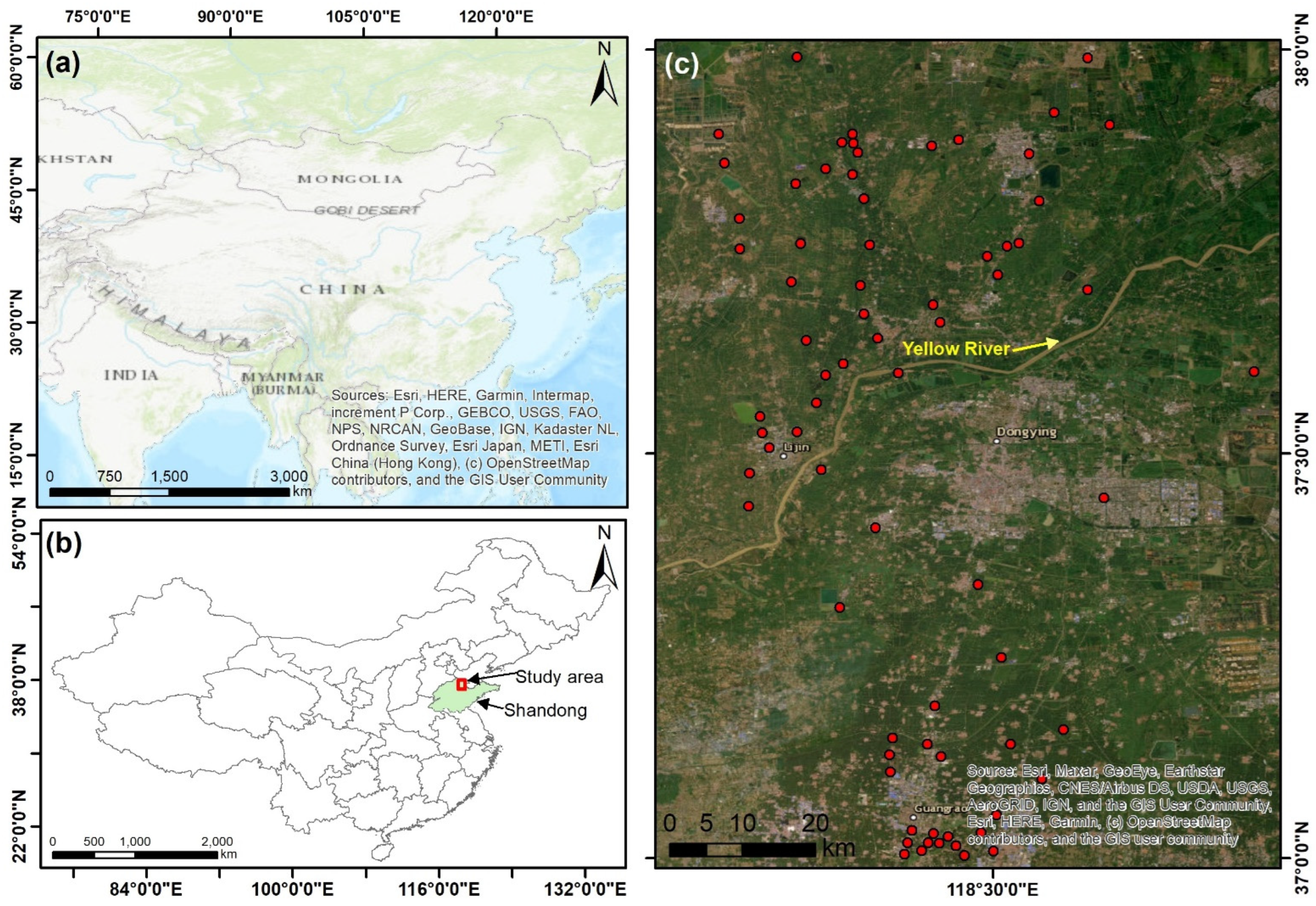
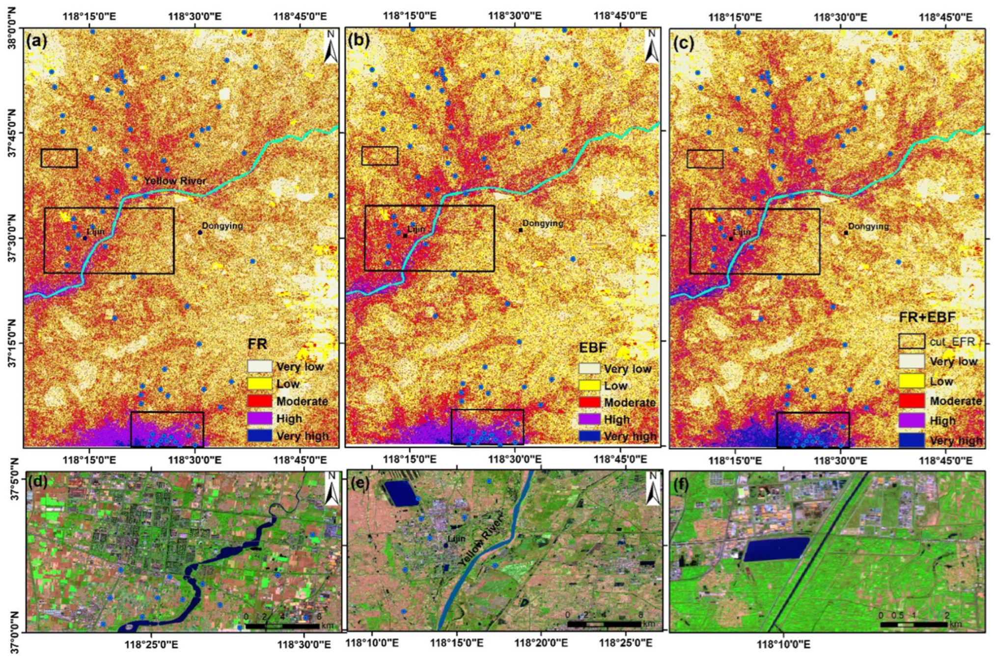
The study area is situated in Shandong Province’s lower sections of the Yellow River, and it borders the Bohai Sea to the east (Figure 1), covering about 7438 km². The muddy waters of the Yellow River give the area its name. In 1958, 2.1 billion tons of silt were dumped into the ocean, and every year since, around 30 km² of new land forms. This region experiences a warm temperate semi-humid monsoon climate. The annual average rainfall is between 530 and 630 mm, which is considerably less than the yearly average evaporation of between 1470 and 2246 mm [70,71]. In western Shandong, the Yellow River flows along a levee that is higher than the surrounding landscape. After traversing various regions of the province, it drains into the sea around Shandong’s northern shore. The topography of the area is characterized by steep hills in the southwest and level terrain in the northeast. The alluvial marine plains in the coastal locations have a ground elevation of only 2–5 m, compared with the northern Shandong hills, with elevations around 10–30 m [48]. The average temperature ranges from 5 to 1 °C (from 23 to 34 °F) in January and from 24 to 28 °C (from 75 to 82 °F) in July. The two main methods for shallow groundwater recharging are precipitation and river infiltration. The Quaternary sediment thickness in the current study area is about 350 m, and the Holocene marine and deltaic sediment thickness is about 26 m [71].

3. Data Used and Methods

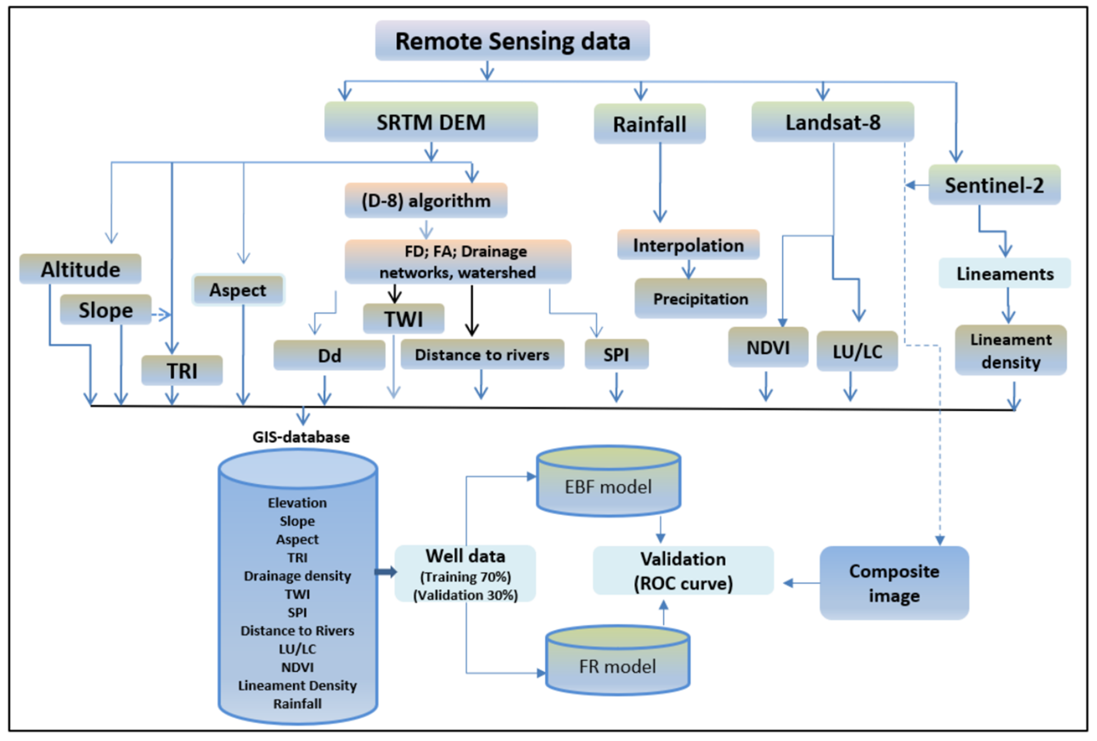
In this study, we integrated remote sensing data from a variety of sensors with topographic, hydrologic, and meteorological data to depict the possible water resource locations. We used GIS techniques to merge several thematic maps (elevation, slope, aspect, terrain roughness index, SPI, lineaments, drainage density, distance to river, TWI, NDVI, LU/LC, and rainfall intensity) produced from these data. These twelve factors are important contributors to groundwater occurrence that represent the climatic, hydrologic, land-cover, and topographic factors. We describe these factors in Section 4. We present the identification approaches of the FR and EBF models used to map the groundwater potential zones in Figure 2.

We initiated the digital elevation models (DEMs) using SRTM (Shuttle Radar Topography Mission) data (90 m cell size). We used the Shuttle Radar Topographic Mission SRTM 30 m resolution NASADEM 1 arc second WGS84 data to examine the topographic changes (NASADEM 1 arc second WGS84). The DEMs allowed for the extraction of the slope, aspect, and TRI. We produced the stream network using the 8D approach [72], and we used a GIS application to produce the stream density map, TWI, SPI, and distance to rivers. We calculated the distances to rivers using the Euclidean distance spatial tool in ArcGIS.

Landsat 8, which was deployed on 11 February 2013, carries the operational land imager (OLI) and thermal infrared sensor (TIRS). In the mapping of the land cover and use, the visible-near-infrared and shortwave-infrared wavelength ranges are used. A Landsat-8 OLI scene (path 121/row 034) that was acquired on 30 December 2021 underwent image alterations and enhancement procedures. We stacked bands 2, 3, 4, 5, and 7 to a 30 m spatial resolution and projected them to WGS-84, UTM Zone 50 N. We used the data from Landsat 8 to reveal the vegetation and water resource signatures. We computed the normalized difference vegetation index (NDVI) to reveal the vegetation areas [25], and we estimated them by applying the visible infrared bands (NDVI = NIR (band 5) − R (band 4) and NIR (band 5) + R (band 4)). In addition to Landsat OLI, we used a Landsat-5 scene (path 121/row 034) that was acquired on 24 August 1992 (bands 7, 4, and 2 in R, G, and B, respectively) in the change detection in the present study (

Table 1. Data used in present study.

No	Type of Data	Source	Date	Resolution
1	Landsat-8 OLI	USGS	30 December 2021	bands 2, 3, 4, 5, 6, and 7 (30 m)
2	Sentinel-1	ESA/Copernicus	18 October 2022	bands 2, 3, 4, 8, (“10” m, 11, and 12 (“20” m)
3	SRTM DEM	USGS	11–22 February 2000	C-band (30 m)
4	Climatic Research Unit data	crudata.uea.ac.uk	1 January 2011–1 January 2020	0.5 degrees in latitude and longitudes

).

The Sentinel-2A satellite was launched on 23 June 2015, and the first data were collected a few days later. The Sentinel-2 sensors collect the VNIR, SWIR, and TIR data. The spatial resolution of these bands is 10–60 m. Sentinel-2 records a total of 13 bands of the VNIR and SWIR spectra. The coastal B1 (443 nm) band has a 60 m pixel geometry; however, the VNIR blue B2 (490 nm), green B3 (560 nm), red B4 (665 nm), and infrared B8 (842 nm) bands have 10 m pixels. The SWIR bands (B11: 1610 nm; B12: 2190 nm) have 20 m wide pixels. Sentinel-2 satellites have temporal resolutions of 10 and 5 days, which makes them extremely valuable for future investigations. Sentinel-2 scenes are delivered as zip-compressed files in Sentinel’s own SAFE format. The spectral bands are stored as jpg files in this SAFE file at three different geometric resolutions (10, 20, and 60 m). The jpg files of bands B2, B3, B4, and B8, with spatial resolutions of 10 m, and of bands B11 and B12, with 20 m resolutions, are stacked into a single GeoTIFF file of a uniform pixel size (10 m). We obtained a subset of these data during preprocessing using SNAP software to minimize the computational time and data. We extracted the LC/LU differences using images from two dates (3 November 2018 and 18 October 2022).

The Climatic Research Unit obtained the data on the average rainfall with a 0.5° resolution. The period covered by the collected average rainfall data spanned from January 2011 to 2020, and we interpolated them using the kriging tool of Arc GIS (https://crudata.uea.ac.uk/cru/data/hrg/ accessed on 01 November 2022).

In this study, we applied the data-driven application of the EBF and FR methodologies to obtain more accurate estimates of the potential groundwater areas. We compared the EBF results with the results of well-known statistical methods, including logistic regression (LR) and the frequency ratio (FR). The EBF model produces better results in terms of groundwater [50] and flood hazards [73], and it produces better results over fuzzy logic models in mapping landslides [74]. Moreover, it produces better results in revealing land subsidence [75]. We can use the model to analyze the effects of all classes of each factor and the correlation between each component, which gives it an advantage over other statistical methods [73]. Additionally, the frequency ratio (FR) is one of the better-known statistical methods [76], and it is more efficient and dependable than the knowledge-driven AHP model [77].

We produced the groundwater potential map using a data-driven FR–EBF model built on a geographic information system (GIS), and we set or resampled all the input data to a 30 m resolution following the spatial resolution of digital elevation data. In numerous prediction techniques, researchers frequently employ this kind of multicriterion decision-making process. The user chooses the relative importance of each observation in the model, which is based on remote sensing, hydrologic, and geologic data. In the GIS approach, a raster combination is used in which each layer’s pixel is associated with a particular geographic location. As a result, the combination process is more suited to the integration of traits from several datasets into an output layer. Moreover, for each pixel in the study area, we can calculate the GWPZ indices using the EBF model. We calculated the likelihood of a well occurrence in each unit cell to infer the spatial relationship between the wells and each thematic evidentiary layer. To calculate the data-driven EBF application, we used the number of well cells (with at least one cell) in each evidentiary layer.

The frequency ratio (FR) model, which is used to represent the incidence probability for a specific attribute, is a straightforward geospatial assessment tool that we can use to ascertain the final relationship between the GRW potential and its effective factors [62,68]. To determine the frequency ratio and to apply it to the overall recharge, we determined the recharge occurrence ratio for each subclass of conditioning factors. We calculated the surface ratio for each class and measured it against the total watershed area in Step 9. We calculated the FR values for each subclass of GWR potential effective factors based on how well they correlated with the GWR potential inventory.

4. Results

4.1. Elevation

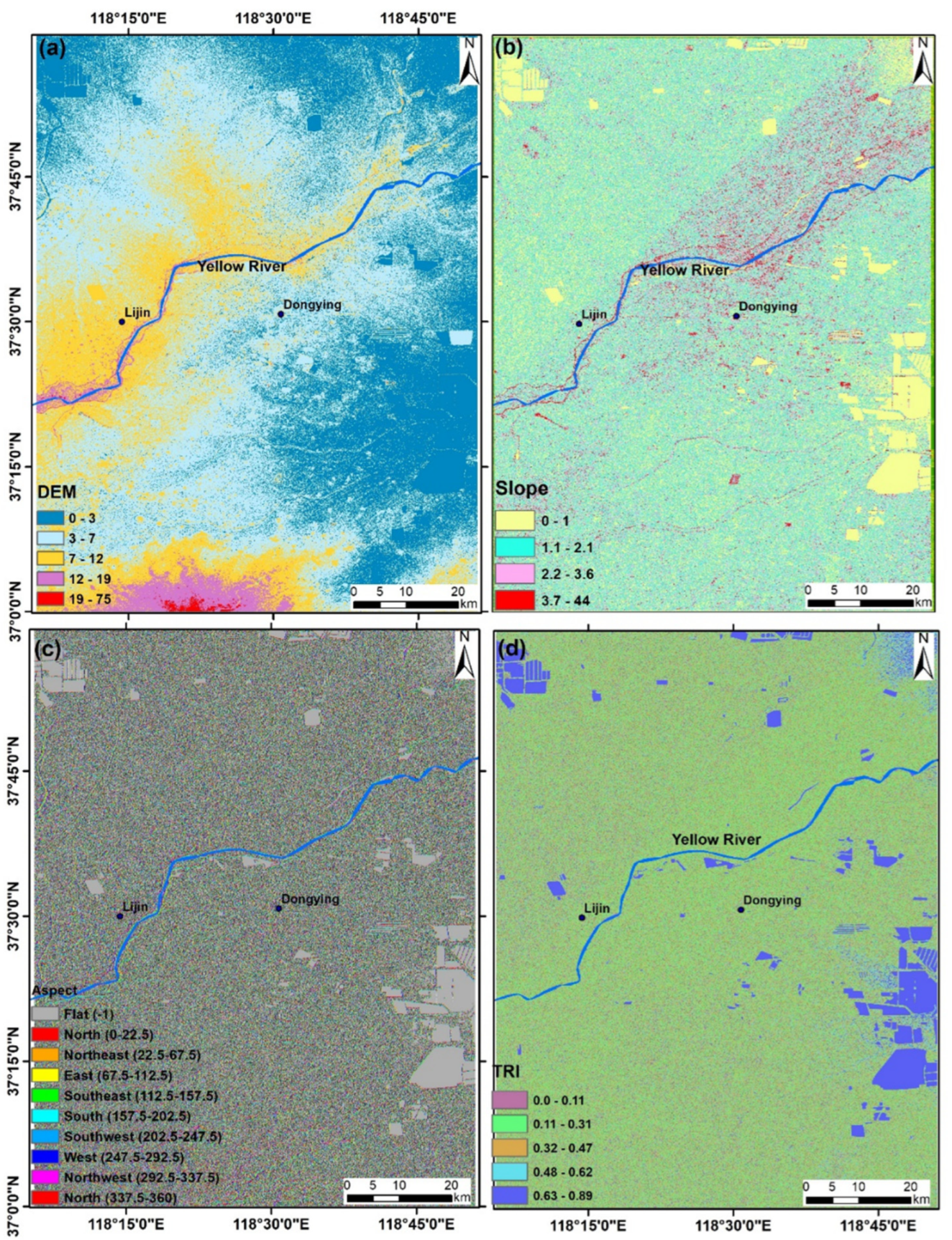
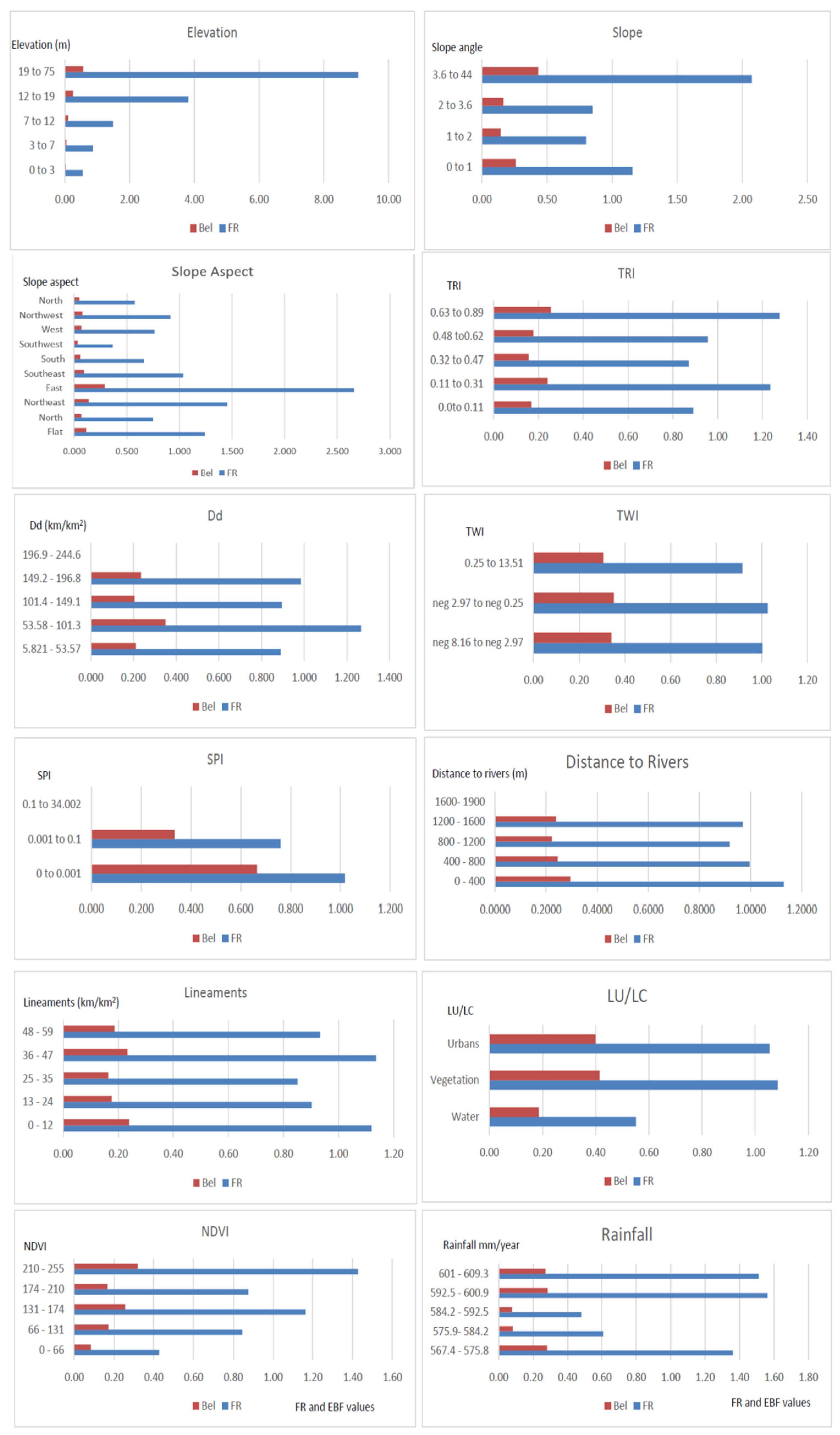
The elevation is a topographical feature that is used as a surface indication to investigate the groundwater potential. Elevation change can affect the climate, which can change the rainfall, soil quality, vegetation, land uses, and vegetation types [62]. The elevation is an important layer that governs the direction of the water flow over the land, and it controls the groundwater occurrence and recharge potential [78]. We categorized the elevation map of the study area (Figure 3a) into five zones: (1) 0–3; (2) 3–7; (3) 7–12; (4) 12–19; (5) 19–75, which covered 29.35, 48.04, 19.55, 2.86, and 0.20% of the entire basin, respectively.

4.2. Slope

The slope is one of the indications of prospective groundwater occurrences, and the topography and/or slope gradient have a direct impact on how much rainwater is infiltrated [79]. Additionally, the slope can provide a general indication of the groundwater movement direction [80]. While a moderate-to-steep slope increases the runoff water, a low or almost level slope has a high infiltration rate and little runoff, which leads to good groundwater recharging [81]. We can determine the slope via either digital elevation models from physical measurements, such as STRM DEMs [82,83,84,85], or from survey base points and topographical contours, both of which allow for the creation of a DEM [63]. We classified the slope angles of the study area, which ranged from 0 to 44 degrees, into four classes: (1) 0–1; (2) 1–2; (3) 2–3.6; (4) 3.6–44 (Figure 3b), which covered 40.87, 36.36, 19.26, and 3.51% of the entire area, respectively (Table 1). Areas with low slope angles are groundwater potential areas with high potentiality; however, steep slopes promote runoff [86].

4.3. Aspect

The infiltration rate is substantially influenced by the slope aspect, which also affects the GWR, which is a measure of the solar radiation. The slope aspect, which ranges from 0 to 360 degrees in a clockwise rotation, is the slope’s orientation. We created the slope factor using the DEM in ArcGIS 10.6, and we used the DEM in ArcGIS 10.8 to calculate the aspect. The aspect measurements included ten categories: (1) flat (or no aspect direction); (2) north; (3) northeast; (4) east; (5) southeast; (6) south; (7) southwest; (8) west; (9) northwest; (10) north. The northern hemisphere has more water resources on the slopes that face north and east than on the slopes that face south and west. The slopes of the mountains to the east and north receive less sunshine than the slopes to the south and west [87]. Despite the high soil moisture levels on the slopes that face north and east, the transpiration is modest, and vegetation has increased on the northern and eastern faces as a result. An increase in vegetation can improve the surface infiltration and groundwater recharge in some areas [26,87]. We divided the aspect map (Figure 3c) into ten classes: (1) flat (−1); (2) N (0–22.5); (3) NE (22.5–67.5); (4) E (67.5–112.5); (5) SE (112.5–157.5); (6) S (157.5–202.5); (7) SW (202.5–247.5); (8) W (247.5–292.5); (9) NW (292.5–337.5); (10) north (337.5–360), which covered 8.77, 9.68, 8.74, 8.89, 10.52, 8.24, 9.91, 9.49, 9.91, and 15.84% of the entire area, respectively.

4.4. TRI

The topography roughness index (TRI), which is a geomorphometric statistic that we used to describe and quantify the spatial distributions of the hills and valleys in the research area, also has an impact on the groundwater potential. The TRI was created to assess landscape heterogeneities, and we can use it to identify groundwater [4,88]:

$$TRI=\sqrt{(ma{x}^2}-mi{n}^2)$$

(1)

We classified the TRI result map of the study area, which ranged from 0 to 0.89, into five classes: (1) 0.00–0.11; (2) 0.11–0.31; (3) 0.32–0.47; (4) 0.48–0.62; (5) 0.63–0.89 (Figure 3d), which covered 6.12, 8.84, 31.30, 38.06, and 15.68% of the entire area, respectively (Table 1).

4.5. Drainage Density (Dd)

Drainage is a crucial hydrogeological control mechanism. Surface and subsurface structures are reflections of drainage patterns [89,90], while the relationship between the permeability and drainage density is inverse. The type of vegetation, the soil’s ability to absorb rainwater, infiltration, and the slope gradient are all factors that influence an area’s drainage system. The bedrock type and structure also have impacts [91]. When there is a high drainage density in a low-permeable-surface region, there is also high precipitation runoff from that area [89,92]. A high-drainage-density zone contributes to a high amount of surface runoff with a low groundwater recharge volume [93,94], and the overall length of the drainage densities correlates with the groundwater recharge volume [95]. Areas with less drainage density have greater infiltration and less surface runoff, which means that groundwater development is appropriate in places with low drainage densities [96,97]. Furthermore, because it is used to measure the surface runoff, the drainage density indirectly reveals the groundwater recharge [98]. Low infiltration and higher surface runoff due to a high Dd result in lower groundwater potential [63,99]. We classified the Dd result map of the study area, which ranged from 5.82 to 244.6, into five classes: (1) 5.82–53.57; (2) 53.58–101.3; (3) 101.3–149.1; (4) 149.1–196.8; (5) 196.9–244.6 (Figure 4a,b), which covered 12.26, 33.02, 32.53, 18.48, and 3.71% of the entire area, respectively (Table 1).

4.6. Topographic Wetness Index (TWI)

We used the TWI map as an indicator of the slope, elevation, and landform effects on the groundwater resources [100]. In the TWI, the upslope area is an indicator of flowing water (local slope) or a gauge of the subsurface lateral transmissivity [45,50]. The regional diversity of the hydrological conditions, including the soil moisture, substantially depends on the TWI [101]. The extent and zoning of saturated areas are influenced by the TWI, which, in turn, affects the incidence of springs [44,45]; thus, the higher the TWI, the greater the groundwater potential [7]. The TWI calculations include a summary of the topographic roughness, hillslope, and foothill effects on the lateral groundwater flow [102]. Areas with high TWIs allow us to locate areas with infiltration potential and soil moisture accumulation, which are unusual in foothills [103,104].

$$TWI=\ln (\frac{Ac}{tans})$$

(2)

We classified the TWI result map of the study area into three classes: (1) from −8.16 to −2.97; (2) from −2.97 to 0.25; (3) from 0.25 to 13.51 (Figure 4c), which covered areas of 56.19, 31.89, and 11.92% of the entire area, respectively (Table 1).

4.7. SPI

The SPI is an important index for mapping groundwater infiltration zones. The SPI is an indicator of the slope, elevation, and landform effects on the groundwater resources [62]. Using slope and flow accumulation parameters, we computed the SPI using Arc GIS software version 10.5. The runoff influence increased as the SPI value increased [105,106]. We classified the SPI result map of the study area, which ranged from 0 to 34.002, into three classes: (1) 0–0.001; (2) 0.001–0.1; (3) 0.1–34.002 (Figure 4d), which covered areas of 94.67, 4.79, and 0.54% of the entire area, respectively (Table 1).

4.8. Distance to River

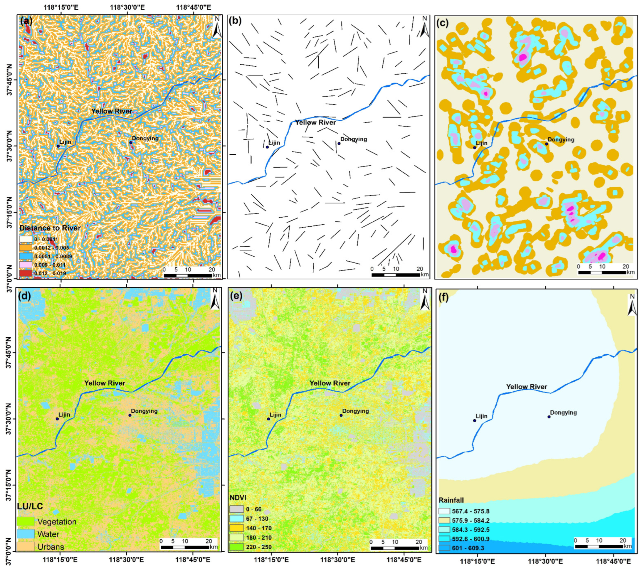
In hydrogeological research, the distance from hydrographic networks is crucial because the local alluvial layers are typically found close to river courses, and especially in semiarid environments [107]. Riverfront locations are ideal for efficient infiltration, and thus, for groundwater recharge [44,55]. The groundwater potential is stronger in areas near rivers, and particularly those with continuous or extended flows [43,59,108]. However, in places farther than 600 m, it is challenging to locate the alluvial layers [4]. Rivers contribute to the GWR, and hence, affect its potential in watersheds. To initiate the distance categories, we utilized the Euclidean distance tool from the spatial analyst tools in Arc GIS 10.6 [62]. We classified the map of the distance to river results of the study area, which ranged from 0 to 0.019, into five classes: (1) 0.00–0.0039; (2) 0.004–0.0078; (3) 0.0079–0.012; (4) 0.013–0.016; (5) 0.017–0.019 (Figure 5a), which covered 28.96, 34.66, 21.77, 31.12, and 1.48% of the entire area, respectively (Table 1).

4.9. Lineaments

Linear earth features that result from geologic structures, which are known as lineaments, serve as overall surface depictions of the subsurface cracks [109]. Geological features with linear or curved shapes play a major role in the occurrence and transport of groundwater over crystalline terrain. Lineaments, such as cracks, fissures, and joints, cause the infiltration of surface runoff and the replenishment of hard-rock aquifers, and they often form because of tectonic stress/strain. Numerous academics have highlighted the connection between lineaments and the presence of groundwater to emphasize how the lineament density affects well yields [110,111,112]. Lineaments fall under the category of secondary porosity, and we can distinguish them from other terrain characteristics on satellite imagery by tonal differences. A lineament can be a fault, fracture, or master joint, or a lengthy linear geological structure, topographic linearity, or a stream’s straight course [113]. Lineaments have a substantial impact on the groundwater storage and flow and surface runoff infiltration into the subsurface [114]. We classified the lineament density map of the study area (Figure 5b,c) into five zones: (1) 0–12; (2) 12–24; (3) 24–35; (4) 35–47; (5) 48–59, which covered 34.09, 22.17, 23.50, 14.40, and 5.84% of the entire basin, respectively. We gave dense lineament zones that were deemed potential groundwater recharge zones and that promoted well production to a higher rank (“numeric value”).

4.10. Land Use/Cover

Land use/cover includes a region’s vegetation cover, aquatic bodies, residential neighborhood distribution, urbanization, and soil deposit types [115]. Land use/cover has a substantial impact on the groundwater recharge, occurrence, and availability [116,117]. For instance, agricultural and plantation lands are good locations for groundwater investigations because trees and plants can collect water on their foliage and allow it to seep into the earth through their roots and biological processes, which replenishes the water table [118]. However, because of the usage of concrete floors, which only allow for surface drainage, settlements are poor groundwater areas [85]. Typically, researchers use topographic maps and a combination of field verification and remotely sensed data to map land-use and land-cover patterns. False color composites (FCCs) are typically created from satellite images utilizing a variety of band combinations [84,119].

The recharge in vegetated areas is substantially lower than that in non-vegetated areas, according to Gee et al. [120]. Furthermore, compared with permanent lands, such as shrub and forest areas, recharging is higher in agricultural and grassland areas [121]. To identify the different types of LUs, we used Landsat-8 data. Additionally, using a supervised classification strategy and the maximum likelihood approach, we classified the LU/LC result map of the study area into three classes: (1) water, (2) vegetation, and (3) urban (Figure 5d), which covered 13.19, 20.24, and 46.57% of the entire area, respectively (Table 1).

4.11. NDVI

Researchers frequently use the NDVI for groundwater potential zones [122,123]. Using a map of the normalized difference vegetation index (NDVI), we depicted the vegetation density and coverage. We used Envi 5.3 to prepare the NDVI layer. The NDVI has a value range from −1 to 1 (often known as from 0 to 255). A greater NDVI value indicates thick vegetation. We classified the NDVI result map of the study area, which ranged from 0 to 255, into five classes based on the natural breaks method: (1) 0.00–66; (2) 66–131; (3) 131–174; (4) 174–210; (5) 210–255 (Figure 5e), which covered 8.52, 8.61, 28.13, 39.45, and 15.28% of the entire area, respectively (Table 1).

4.12. Rainfall

The rainfall amount is one of the key elements in the identification of groundwater potential zones. Rainfall is a hydrologic technique for refilling aquifers [97]. The groundwater likelihood in a given land area increases with the rainfall [124]. Researchers can track, observe, and measure the analyzed watershed’s downpour rates using rainfall data from the TRMM satellite. Due to the substantial precipitation and subsequent flooding from storms, the infrastructure in the area has been severely damaged, and there have been losses in the provision of water resources. The identification of areas that are prone to water accumulation may be possible using rainfall information because precipitation is crucial for recharging groundwater [125]. We classified the mean annual rainfall intensity (2011–2020) map of the study area (Figure 5f) into five zones: (1) 567.4–575.8; (2) 575.9–584.2; (3) 584.3–592.5; (4) 592.6–600.9; (5) 601–609.3, which covered 32.05, 38.89, 11.33, 9.31, and 8.42% of the entire basin, respectively. We gave the dense rainfall zones that were deemed potential groundwater recharge zones and that promoted well production to a higher rank (“numeric value”).

5. Results

5.1. Application of FR Model

Researchers use the FR to describe the likelihood that a phenomenon possesses a particular characteristic [28]. We entered the calibration well locations (the dependent variable) and conditioning factors (such as the lithology, slope, distance to streams, and distance to faults) using the FR approach [126]. We calculated the well occurrence chance in each class for all the parameters using the FR [28]. We used the following equation to determine each class’s impact on the independent variable:

$$\mathrm{Fr}=\frac{\left(P_t/T{p}_t\right)}{\left(N_c/T_{Nc}\right)}$$

(3)

where FR is the rate at which each class of each parameter impacts the parameter; P_t denotes the proportion of points in each class; T_pt is the total number of points across all classes; N_C is the number of classes; T_NC is the total number of pixels. The FR value produced for each class of conditioning factors determines the weight of each class of conditioning factors in the subject layers for mapping the groundwater potential. After applying the FR to each class, the new thematic layer is the input value for the hybrid model.

We identified the spatial correlations between the well locations (a proxy for the groundwater potential) and conditioning factors using the FR model (Table 1). According to Lee and Pradhan [127], FR values below 1 indicate low correlations, and those above 1 indicate strong correlations. The elevation classes from 19 to 75 had the highest FRs (9.06), followed by the elevation classes from 12 to 19 (3.81), from 7 to 12 (1.48), from 3 to 7 (0.87), and from 0 to 3 (0.55). Because this range indicates a flat plateau, the areas with high elevations (between 19 and 75) are more likely to retain groundwater. The zones with slopes from 0 to 1 had high FRs (1.157), as did the E, NE, Flat, and SE zones (2.65, 1.45, 1.24, and 1.03, respectively), as the area’s general slope is due east. Additionally, the areas with higher TRIs (from 0.63 to 0.89) and low terrains (from 0.11 to 0.31) had FRs of 1.27 and 1.23, respectively.

In terms of the hydrologic characteristics, the zones with low Dd values (from 53.58 to 101.3) had higher FRs (1.26); however, the areas of high Dd values had the lowest FRs (Table 1). The groundwater potential probability was the highest for the TWI class from −2.97 to 0.25 (FR = 1.026), followed by the TWI classes from −8.16 to 2.97 (FR = 1.003) and from 0.25 to 13.51 (FR = 0.915). The SPI classes from 0.0 to 0.001 (FR = 1.018) and from 0.001 to 0.1 (FR = 0.760) had high probabilities; however, the areas of high SPIs (from 0.1 to 34.002) had no potentiality (FR = 0). Furthermore, the areas nearest to the rivers from 0 to 0.0039 had the highest FRs (1.130), followed by those from 0.004 to 0.0078 (0.997); however, the areas farther from the rivers had no potentiality (FR = 0).

The lineament density values from 36 to 47 (FR = 1.136) were the highest, followed by those from 0 to 12 (FR = 1.120); however, the moderate LD areas (from 25 to 35) had the lowest FR values (FR = 0.851). Using the LU/LC, the groundwater potential probability was the highest for the vegetation class (FR = 1.08), as well as for areas with high NDVIs (from 210 to 255) (FR = 1.42); however, the areas from 0 to 66 had low GWPs (FR = 0.427). In terms of the rainfall classes, the areas that received from 114.42 to 148.13 mm had the highest precipitation (FR = 1.56), followed by those that received from 148.13 to 244.56 mm (FR = 1.512) and from 570 to 580 mm (FR = 1.36); however, the areas that received from 580 to 590 mm had the lowest FRs (0.608).

5.2. Application of EBF Model

For the spatial prediction of possible groundwater areas, we used the Dempster–Shafer-based evidential belief function (EBF) [128,129,130]. This strategy is a potentially effective way to address some of the challenges that are associated with the combination of evidence and data fusion [131]. We can calculate the EBF as follows [132]:

$$\mathrm{BeI}{C}_{ij}=\frac{1W_{C_{ij}D}}{{{\displaystyle \sum }}_j^m=1W_{C_{ij}D}}$$

(4)

$$W_{C_{ij}D}=\frac{N\left(C_{ij}{{\displaystyle \cap }}^{\hspace{1em}}D\right)/N\left(C_{ij}\right)}{N\left(D\right)-N\left(C_{ij}{{\displaystyle \cap }}^{\hspace{1em}}D\right)/N\left(T\right)-N\left(C_{ij}\right)]}$$

(5)

The numerator used to calculate the $W_{C_{ij}D}$ is the likelihood that the D (groundwater) occurs in the presence of C_ij (a particular class of one conditioning factor), which demonstrates that the D more frequently occurs (or is more present) in the C_ij than would be predicted by chance. The denominator used to calculate the $W_{C_{ij}D}$ is the conditional probability that D exists given the lack of C_ij, which indicates that D more frequently occurs outside of C_ij than would be predicted by chance. Therefore, the parameter $W_{C_{ij}D}$ is the weight of the C_ij in terms of D being more present than absent as anticipated by chance. Therefore, the relative strength of the $W_{C_{ij}D}$ for each j^th C_ij class of evidence in map Xi is BeI C_ij, as indicated in the equations above. N (Cij∩D) represents the number of wells that occur in a subclass; N (Cij) is the number of pixels in a subclass; N (D) is the total number of wells; N (T) is the sum of the pixel domain for a class. Accordingly, for the $W_{C_{ij}D}$, we can calculate the BeI Cij, as shown in Table 1. The values of the Bel range are between 0 and 1 for each subclass.

The groundwater potential probability was the highest for the elevation classes from 19 to 75 m with the highest EBFs (0.565); however, it was the lowest for the elevation classes from 0 to 3 m (EBF = 0.029) (

Table 2. Groundwater factors of the adopted models in the study area.

Topography	No. Pixels in Domain	Domain %	No. Wells	No. Wells %	FR	N (Cij∩D)/N (Cij)	N (D) −N (Cij∩D)	N (T) −N (Cij)	N (D) −N (Cij∩D)/N (T) −N (Cij)	WcijD	Bel
0 to 3	2,883,463	0.29345745	9	0.164	0.558	0.0000031	46	6,942,367	6.62598 × 10−6	0.471	0.029
3 to 7	4,720,324	0.48039952	23	0.418	0.870	0.0000049	32	5,105,506	6.26774 × 10−6	0.777	0.048
7 to 12	1,921,284	0.19553402	16	0.291	1.488	0.0000083	39	7,904,546	4.93387 × 10−6	1.688	0.104
12 to 19	281,047	0.02860288	6	0.109	3.814	0.0000213	49	9,544,783	5.13369 × 10−6	4.159	0.255
19 to 75	19,712	0.00200614	1	0.018	9.063	0.0000507	54	9,806,118	5.50677 × 10−6	9.212	0.565
Slope
0 to 1	4,010,495	0.40868454	26	0.473	1.157	0.0000065	29	5,802,685	4.99769 × 10−6	1.297	0.260
1 to 2	3,568,474	0.36364094	16	0.291	0.800	0.0000045	39	6,244,706	6.24529 × 10−6	0.718	0.144
2 to 3.6	1,889,910	0.19258895	9	0.164	0.850	0.0000048	46	7,923,270	5.80568 × 10−6	0.820	0.164
3.6 to 44	344,301	0.03508557	4	0.073	2.073	0.0000116	51	9,468,879	5.38607 × 10−6	2.157	0.432
Slope ASPECT
Flat	860,817	0.08772049	6	0.109	1.244	0.0000070	49	8,952,363	5.47342 × 10−6	1.273	0.117
North	950,349	0.09684414	4	0.073	0.751	0.0000042	51	8,862,831	5.75437 × 10−6	0.731	0.067
Northeast	857,199	0.08735181	7	0.127	1.457	0.0000082	48	8,955,981	5.35955 × 10−6	1.524	0.140
East	872,576	0.08891878	13	0.236	2.658	0.0000149	42	8,940,604	4.69767 × 10−6	3.171	0.291
Southeast	1,032,724	0.10523847	6	0.109	1.037	0.0000058	49	8,780,456	5.58058 × 10−6	1.041	0.095
South	808,454	0.08238451	3	0.055	0.662	0.0000037	52	9,004,726	5.77475 × 10−6	0.643	0.059
Southwest	972,047	0.09905525	2	0.036	0.367	0.0000021	53	8,841,133	5.99471 × 10−6	0.343	0.031
West	931,399	0.09491307	4	0.073	0.766	0.0000043	51	8,881,781	5.74209 × 10−6	0.748	0.069
Northwest	972,718	0.09912363	5	0.091	0.917	0.0000051	50	8,840,462	5.65581 × 10−6	0.909	0.083
North	1,554,897	0.15844986	5	0.091	0.574	0.0000032	50	8,258,283	6.05453 × 10−6	0.531	0.049
Terrain Roughness Index (TRI)
0.0 to 0.11	602,302	0.06124132	3	0.055	0.891	0.0000050	52	9,232,594	5.63222 × 10−6	0.884	0.169
0.11 to 0.31	869,074	0.08836636	6	0.109	1.235	0.0000069	49	8,965,822	5.4652 × 10−6	1.263	0.241
0.32 to 0.47	3,078,693	0.31303768	15	0.273	0.871	0.0000049	40	6,756,203	5.92049 × 10−6	0.823	0.157
0.48 to0.62	3,743,124	0.3805962	20	0.364	0.955	0.0000053	35	6,091,772	5.74545 × 10−6	0.930	0.177
0.63 to 0.89	1,541,703	0.15675844	11	0.200	1.276	0.0000071	44	8,293,193	5.30556 × 10−6	1.345	0.256
Drainage Density
5.821–53.57	10,128	0.12264619	6	0.109	0.889	0.0005924	49	72,451	0.000676319	0.876	0.210
53.58–101.3	27,266	0.3301808	23	0.418	1.267	0.0008435	32	55,313	0.000578526	1.458	0.350
101.4–149.1	26,864	0.32531273	16	0.291	0.894	0.0005956	39	55,715	0.000699991	0.851	0.204
149.2–196.8	15,257	0.18475642	10	0.182	0.984	0.0006554	45	67,322	0.000668429	0.981	0.235
196.9–244.6	3064	0.03710386	0	0.000	0.000	0.0000000	55	79,515	0.000691693	0.000	0.000
TWI
−8.16 to −2.97	5,514,106	0.56190817	31	0.564	1.003	0.0000056	24	4,299,074	5.5826 × 10−6	1.007	0.341
−2.97 to −0.25	3,128,986	0.31885546	18	0.327	1.026	0.0000058	37	6,684,194	5.53545 × 10−6	1.039	0.352
0.25 to 13.51	1,170,088	0.11923637	6	0.109	0.915	0.0000051	49	8,643,092	5.66927 × 10−6	0.904	0.307
SPI
0 to 0.001	9,290,340	0.94672063	53	0.964	1.018	0.0000057	2	522,840	3.82526 × 10−6	1.491	0.665
0.001 to 0.1	469,594	0.0478534	2	0.036	0.760	0.0000043	53	9,343,586	5.67234 × 10−6	0.751	0.335
0.1 to 34.002	53,246	0.00542597	0	0.000	0.000	0.0000000	55	9,759,934	5.63528 × 10−6	0.000	0.000
Dist to Rivers
0–400	23,750	0.28963768	18	0.327	1.130	0.0007579	37	58,249	0.000635204	1.193	0.294
400–800	28,423	0.34662618	19	0.345	0.997	0.0006685	36	53,576	0.000671943	0.995	0.246
800–1200	17,855	0.21774656	11	0.200	0.918	0.0006161	44	64,144	0.000685957	0.898	0.222
1200–1600	10,759	0.13120892	7	0.127	0.970	0.0006506	48	71,240	0.000673779	0.966	0.238
1600–1900	1212	0.01478067	0	0.000	0.000	0.0000000	55	80,787	0.000680803	0.000	0.000
Lineaments
0–12	3,273,187	0.34086999	21	0.382	1.120	0.0000064	34	6,329,263	5.37187 × 10−6	1.194	0.240
13–24	2,128,686	0.22168155	11	0.200	0.902	0.0000052	44	7,473,764	5.88726 × 10−6	0.878	0.176
25–35	2,256,503	0.23499242	11	0.200	0.851	0.0000049	44	7,345,947	5.9897 × 10−6	0.814	0.163
36–47	1,382,833	0.14400835	9	0.164	1.136	0.0000065	46	8,219,617	5.59637 × 10−6	1.163	0.234
48–59	561,241	0.05844769	3	0.055	0.933	0.0000053	52	9,041,209	5.75144 × 10−6	0.929	0.187
Land cover
Water	1,090,317	0.13192203	4	0.073	0.551	0.0000037	51	7,174,542	7.10847 × 10−6	0.516	0.186
Vegetation	3,325,930	0.40241824	24	0.436	1.084	0.0000072	31	4,938,929	6.27666 × 10−6	1.150	0.415
Urbans	3,848,612	0.46565973	27	0.491	1.054	0.0000070	28	4,416,247	6.34023 × 10−6	1.107	0.399
NDVI
0–66	729,152	0.08520368	2	0.036	0.427	0.0000027	53	7,828,600	6.77005 × 10−6	0.405	0.084
66–131	736,815	0.08609913	4	0.073	0.845	0.0000054	51	7,820,937	6.52096 × 10−6	0.833	0.172
131–174	2,407,709	0.2813483	18	0.327	1.163	0.0000075	37	6,150,043	6.01622 × 10−6	1.243	0.257
174–210	3,376,062	0.39450337	19	0.345	0.876	0.0000056	36	5,181,690	6.94754 × 10−6	0.810	0.167
210–255	1,308,014	0.15284551	12	0.218	1.427	0.0000092	43	7,249,738	5.93125 × 10−6	1.547	0.320
Rainfall
567.4–575.8	2,944,227	0.32047756	24	0.436	1.362	0.0000082	31	6,242,772	4.96574 × 10−6	1.642	0.282
575.9–584.2	3,573,148	0.38893528	13	0.236	0.608	0.0000036	42	5,613,851	7.4815 × 10−6	0.486	0.083
584.2–592.5	1,041,162	0.11332994	3	0.055	0.481	0.0000029	52	8,145,837	6.38363 × 10−6	0.451	0.077
592.5–600.9	855,039	0.09307054	8	0.145	1.563	0.0000094	47	8,331,960	5.64093 × 10−6	1.659	0.285
601–609.3	773,423	0.08418669	7	0.127	1.512	0.0000091	48	8,413,576	5.70507 × 10−6	1.586	0.272

). The zones with the highest slopes (from 3.6 to 44) and lowest slope angles (from 0 to 1) had the highest EBFs (0.43 and 0.26, respectively). The east, northeast, and flat zones had the highest EBFs (0.29, 0.14, and 0.11, respectively); however, the southwest zone had the lowest (EBF = 0.095). Furthermore, the higher TRI areas (from 0.63 to 0.89) had high EBFs (0.256). In the case of the Dd, EBF values = 0.35 were higher in the classes of low density (from 53.58 to 101.3). We assigned the highest EBF values to the two TWI classes: from −2.97 to 0.25 (EBF = 0.35) and from −8.16 to −2.97 (EBF = 0.34). Furthermore, we assigned the SPI classes from 0.0 to 0.001 and from 0.001 to 0.1 EBFs of 0.66 and 0.33, respectively, as well as groundwater probabilities. According to the LD, the values from 0 to 12 had the highest EBFs (0.24). Using the LU/LC, the groundwater potential probability was the highest for the vegetation class (EBF = 0.415), as well as for the areas with high NDVIs (from 210 to 255), with the highest EBF 0.32. The class from 592.5 to 600.9 mm had the highest EBF value (0.285).

We evaluated the EBF weights (Bel values) for the conditioning factors and their classes, and according to the results, the trends for the EBF values for the classes were correlated as for the FR values (Figure 6), with the exception of a few classes in the Dd, NDVI, lineaments, and rainfall.

5.3. Groundwater Potential Mapping and Validation of Built Models

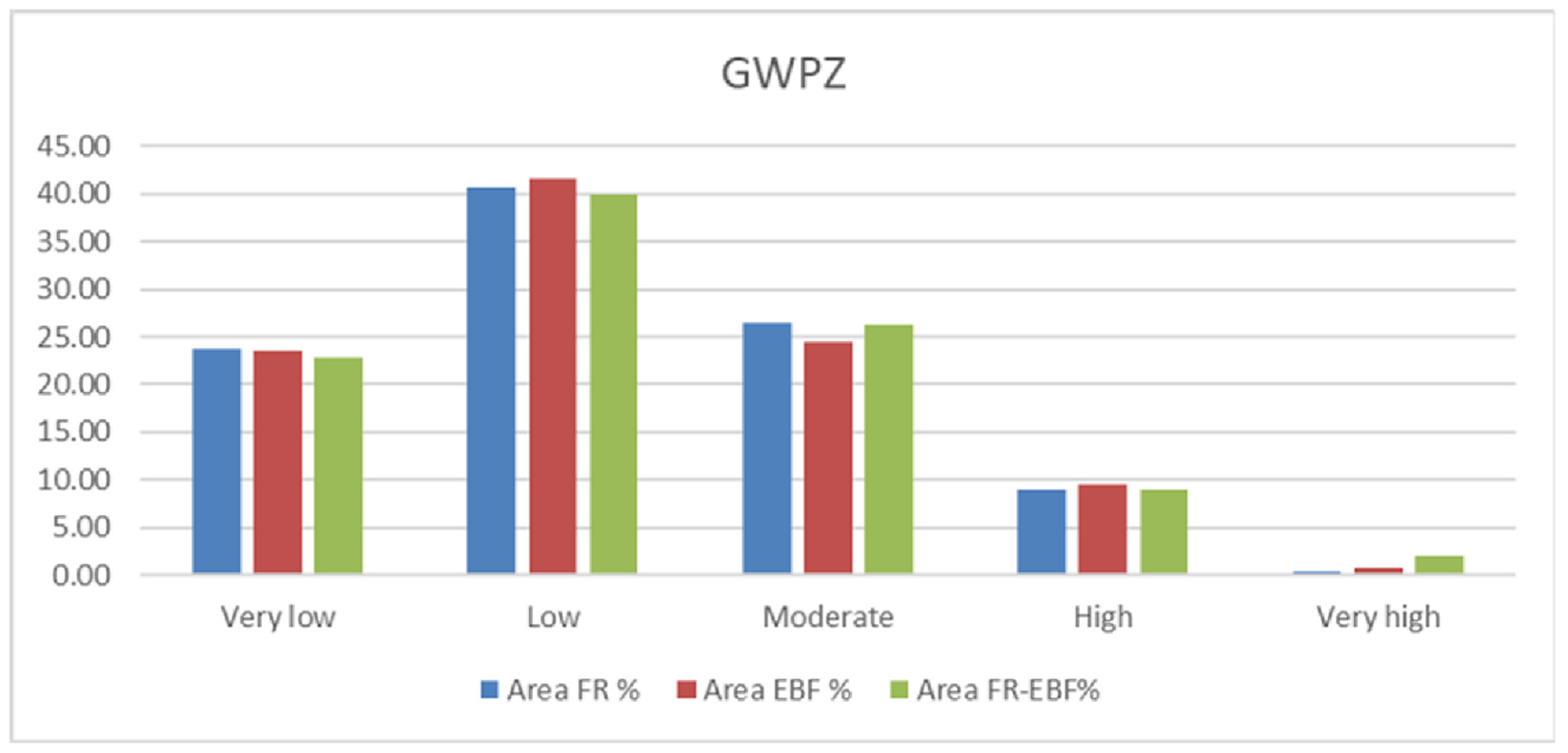
We classified the combined groundwater potential zone (GWPZ) map using the FRs (Figure 7a) combined from twelve thematic maps using the natural breaks approach into five classes: (1) very low (23.67%); (2) low (40.60%); (3) moderate (26.44%); (4) high (8.90%); (5) very high (0.39%). Furthermore, the GWPZ map using the EBF (Figure 7b) that ranged from very low to very high was occupied by 23.60, 41.62, 24.44, 9.57, and 0.78%, respectively. We combined the FR and EBF models to produce the combined FR–EBF model (Figure 7c), which we divided into five classes ranging from very low to very high, and covering areas of 22.89, 39.94, 26.22, 8.98, and 1.97% of the entire area (

Table 3. GWPZ areas.

GWPZ	Area FR %	Area EBF %	Area EBF + FR %
Very low	23.67	23.60	22.89
Low	40.60	41.62	39.94
Moderate	26.44	24.44	26.22
High	8.90	9.57	8.98
Very high	0.39	0.78	1.97

). In the combined FR–EBF model, the areas of the very high and moderate potentiality increased (Figure 8). Based on the Landsat-8 band composites 7, 5, and 3, most of the very high to extreme GWPZs are occupied by vegetation and water resources (Figure 7e,f).

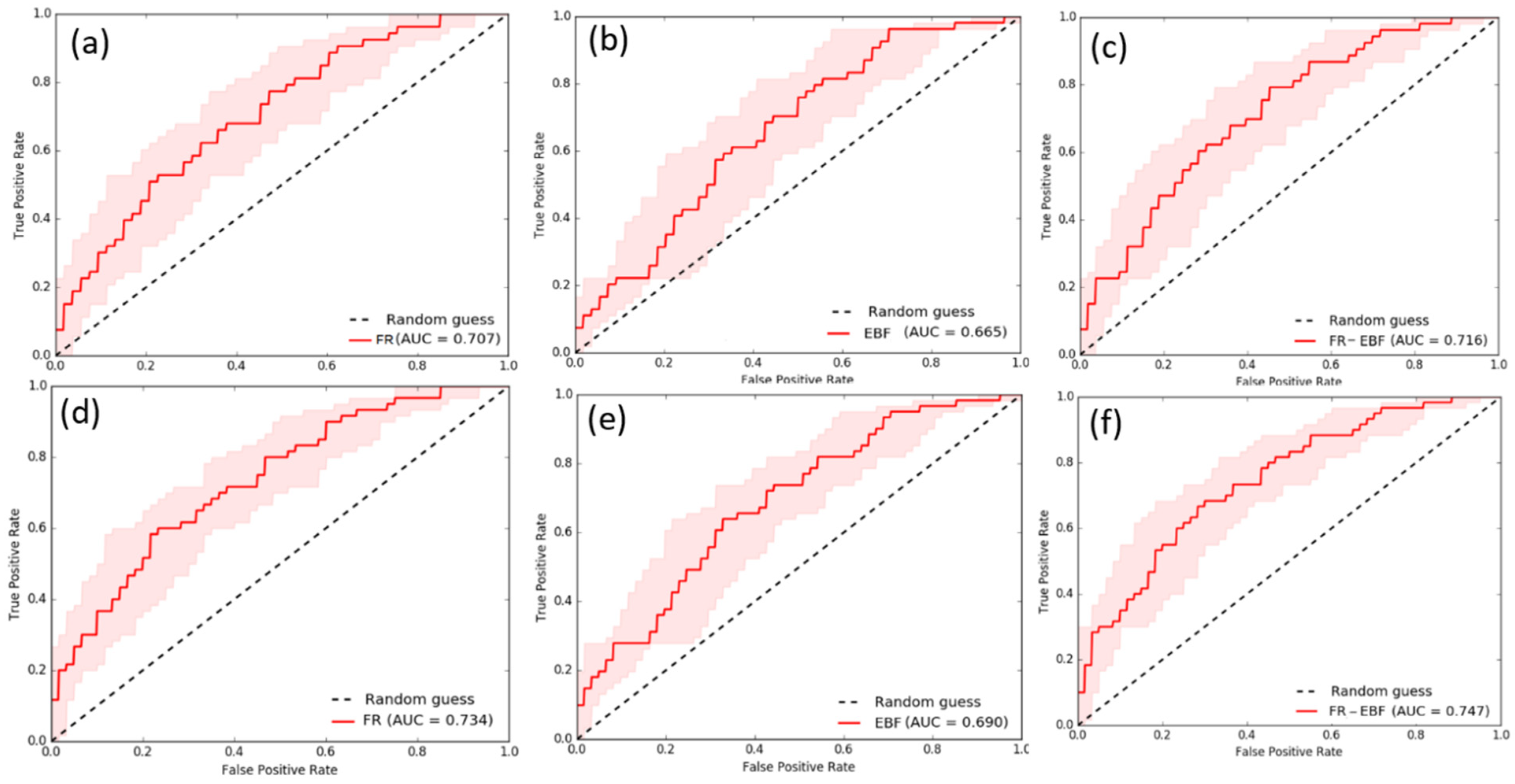
We present the ROC curves for the predicted groundwater map in Figure 8. We can use the AUC to describe the system’s capacity to precisely anticipate both the “groundwater” and “no-existence of groundwater”, which highlights the usefulness of its prediction. The AUC ranges from 0 to 1, with values smaller than 0.5 indicating model integrity, and models with larger values indicating higher accuracy. The AUC results of the models, including the FR, EBF, and combined FR–EBF models, were 0.707, 0.665, and 0.716, respectively. We achieved better accuracy by fusing the two models (the RF–EBF model). Due to the uncertainty around the presence of groundwater in the results, the combined model had better accuracy (AUC = 0.716).

6. Discussion

Water scarcity has now become a major global issue, with substantial implications for the long-term sustainability of water supplies. In the research on spatial groundwater recharge potential zones, researchers emphasize the importance of the efficient planning and management of water resources. According to remote sensing data analyses, GWPZs are controlled by topographic, geomorphic, hydrological, and climatic conditions [28,110,133]. According to the applied FR and EBF models, the rainfall, NDVI, lineament density, and distance to river were positively correlated, and there were more water well locations in the high-altitude areas, which consist of plateaus that are enriched in vegetation and annual precipitation, as well as surface water, near to the Yellow and Zihe Rivers (in the south). The highest well locations were on the east, northeast, and flat slope aspects, which is because the northern hemisphere and north- and east-facing slopes contain more water resources than the south- and west-facing slopes. Less sunlight hits the northern and eastern mountain slopes than it does the southern and western ones. On the north- and east-facing inclines, the transpiration is low despite the high soil moisture levels. The effect is vegetation growth on the northern and eastern faces. In certain places, the increased vegetation enhances the groundwater recharge and surface infiltration [26,87]. The LC/LU types have a substantial impact on the permeability, evapotranspiration, and runoff. The recharge in vegetated areas is substantially lower than that in non-vegetated areas, according to Gee et al. [120]. Furthermore, the recharging is higher in agricultural and grassland areas than on permanent lands, such as shrub and forest areas [121].

The trends of the EBF values for the classes were related to the FR values, according to the evaluation of the EBF weights (Bel values) for the conditioning factors and their classes (Figure 6). The only exception to the similarity were a few classes in the Dd, NDVI, lineaments, and rainfall. The applied FR was better validated than the EBF based on the AUC values of 0.665 and 0.707, respectively. In various studies in the literature, including [75], researchers have demonstrated that the weights generated using the FR and EBF models are consistent [134]. Furthermore, the FR surpasses the EBF techniques, according to numerous studies [28,50]. Combining the two models (FR–EBF model) produced better results than those of each individual model, as validated by the AUC value of 0.716, which was higher than those of the FR and EBF models (Figure 9). Moreover, the combined FR–EBF model increased the areas of very high perspectivity to 1.97, compared with the 0.39 and 0.78 of the FR and EBF models, respectively.

The Yellow River is extensively contaminated by factory waste and sewage from the expanding cities, and hence, it is polluted. The main sources of pollution are industrial, agricultural, and domestic sewage, along with industrial waste gas [135]. Additionally, the increasing wastewater discharge into the river [136] threatens the sustainability of the surface water use. As a result, groundwater has become an appropriate and clean water resource for the long-term sustainability of water supplies in areas with low water quality. Our increasing understanding of the spatial groundwater recharge potential zones highlights the importance of the effective planning and management of water resources [62].

7. Conclusions

In this article, we applied the FR and EBF models, and we integrated them into a hybrid ensemble FR–EBF model that we can use to reveal groundwater potential areas. We prepared, analyzed, and integrated twelve evidential factors. We investigated the spatial recharge based on the topographic, hydrologic, climatic, and land-use elements, and we assessed their potential impacts on GWPZs. According to the findings, the AUC function for the hybrid model (0.716) was reasonably better than those of the individual FR (0.707) and EBF (0.665) models. According to the results, we classified the GWPZs using the natural breaks classifier into five classes that ranged from very low to very high, and that covered areas of 22.89, 39.94, 26.22, 8.98, and 1.97% of the entire area, respectively. The applied modeling techniques and output maps can considerably improve decision makers’ abilities to manage groundwater resources sustainably, to advance efforts to accurately predict the promising areas for extraction and recharge capability. This study presented valuable and better information about the utilize of ensemble FR–EBF model for revealing groundwater potential zones compared with the findings of individual models of FR or/and EBF. Overall, the findings of this study may be applied to the management, planning, and regulation of water resources under various conditions.

References

- Owolabi, S.T.; Madi, K.; Kalumba, A.M. Comparative evaluation of Spatio-temporal attributes of precipitation and streamflow in Buffalo and Tyume Catchments, Eastern Cape, South Africa. Environ. Dev. Sustain. 2020, 23, 4236–4251. [Google Scholar] [CrossRef]
- Owolabi, S.T.; Madi, K.; Kalumba, A.M.; Alemaw, B.F. Assessment of recession flow variability and the surficial lithology impact: A case study of Buffalo River catchment, Eastern Cape, South Africa. Environ. Earth Sci. 2020, 79, 187. [Google Scholar] [CrossRef]
- Abdelkareem, M.; Al-Arifi, N. The use of remotely sensed data to reveal geologic, structural, and hydrologic features and predict potential areas of water resources in arid regions. Arab. J. Geosci. 2021, 14, 704. [Google Scholar] [CrossRef]
- Moghaddam, M.; Rezaei, H.R.; Pourghasemi, Z.S.; Pourtaghie, B.; Pradhan. A Modeling Comparison of Groundwater Potential Mapping in a Mountain Bedrock Aquifer: QUEST, GARP, and RF Models. Arab. J. Geosci. 2015, 8, 913. [Google Scholar] [CrossRef]
- Chaminé, J.M.; Carvalho, M.J.; Afonso, J.; Teixeira, L.; Freitas. On a dialogue between hard-rock aquifer mapping and hydrogeological conceptual models: Insights into groundwater exploration. Eur. Geol. 2013, 35, 25. [Google Scholar]
- Odhiambo, O.G. Water scarcity in the Arabian Peninsula and socio-economic implications. Appl. Water Sci. 2017, 7, 2479–2492. [Google Scholar] [CrossRef] [Green Version]
- Kim, J.C.; Jung, H.-S.; Lee, S. Spatial mapping of the groundwater potential of the geum river basin using ensemble models based on remote sensing images. Remote Sens. 2019, 11, 2285. [Google Scholar] [CrossRef] [Green Version]
- Lee, S.; Hyun, Y.; Lee, S.; Lee, M.-J. Groundwater Potential Mapping Using Remote Sensing and GIS-Based Machine Learning Techniques. Remote Sens. 2020, 12, 1200. [Google Scholar] [CrossRef] [Green Version]
- Hasanuzzaman, M.; Mandal, M.H.; Hasnine; Shit, P.K. Groundwater potential mapping using multi-criteria decision, bivariate statistic and machine learning algorithms: Evidence from Chota Nagpur Plateau, India. Appl. Water Sci. 2022, 12, 58. [Google Scholar] [CrossRef]
- Nguyen, P.T.; Ha, D.H.; Jaafari, A.; Nguyen, H.D.; Van Phong, T.; Al-Ansari, N.; Prakash, I.; Van Le, H.; Pham, B.T. Groundwater Potential Mapping Combining Artificial Neural Network and Real AdaBoost Ensemble Technique: The DakNong Province Case-study, Vietnam. Int. J. Environ. Res. Public Health 2020, 17, 2473. [Google Scholar] [CrossRef] [Green Version]
- Rahmati, O.; Melesse, A.M. Application of Dempster–Shafer theory, spatial analysis and remote sensing for groundwater potential and nitrate pollution analysis in the semi-arid region of Khuzestan, Iran. Sci. Total Environ. 2016, 568, 1110–1123. [Google Scholar] [CrossRef] [PubMed]
- Golkarian, A.; Naghibi, S.A.; Kalantar, B.; Pradhan, B. Groundwater potential mapping using C5.0, random forest, and multivariate adaptive regression spline models in GIS. Environ. Monit. Assess. 2018, 190, 149. [Google Scholar] [CrossRef] [PubMed]
- Barlow, P.M.; Leake, S.A. Streamflow Depletion by Wells: Understanding and Managing the Effects of Groundwater Pumping on Streamflow; US Geological Survey: Reston, VA, USA, 2012.
- Barker, J. A generalized radial flow model for hydraulic tests in fractured rock. Water Resour. Res. 1988, 24, 1796–1804. [Google Scholar] [CrossRef] [Green Version]
- Abdelkareem, M.; El-Baz, F.; Askalany, M.; Akawy, A.; Ghoneim, E. Groundwater prospect map of Egypt’s Qena Valley using data fusion. Int. J. Image Data Fusion 2012, 3, 169–189. [Google Scholar] [CrossRef]
- Elbeih, S.F. An overview of integrated remote sensing and GIS for groundwater mapping in Egypt. Ain Shams Eng. J. 2015, 6, 1–15. [Google Scholar] [CrossRef] [Green Version]
- Dušek, P.; Velísková, Y. Comparison of the MODFLOW modules for the simulation of the river type boundary condition. Pollack Period. 2017, 12, 3–13. [Google Scholar] [CrossRef]
- Zhu, Q.; Abdelkareem, M. Mapping Groundwater Potential Zones Using a Knowledge-Driven Approach and GIS Analysis. Water 2021, 13, 579. [Google Scholar] [CrossRef]
- Rahmati, O.; Naghibi, S.A.; Shahabi, H.; Bui, D.T.; Pradhan, B.; Azareh, A.; Rafiei-Sardooi, E.; Samani, A.N.; Melesse, A.M. Groundwater spring potential modelling: Comprising the capability and robustness of three different modeling approaches. J. Hydrol. 2018, 565, 248–261. [Google Scholar] [CrossRef]
- Shenga, Z.D.; Baroková, D.; Šoltész, A. Modeling of groundwater extraction from wells to control excessive water levels. Pollack Period. 2018, 13, 125–136. [Google Scholar] [CrossRef]
- Mandel, S. Groundwater Resources: Investigation and Development; Elsevier: Amsterdam, The Netherlands, 2012. [Google Scholar]
- Waikar, M.L.; Nilawar, A.P. Identification of groundwater potential zone using remote sensing and GIS technique. Int. J. Innov. Res. Sci. Eng. Technol. 2014, 3, 12163–12174. [Google Scholar]
- Thompson, S.A. Hydrology for Water Management; CRC Press: Boca Raton, FL, USA, 2017. [Google Scholar]
- Abdelkareem, M.; El-Baz, F. Analyses of optical images and radar data reveal structural features and predict groundwater accumulations in the central Eastern Desert of Egypt. Arab. J. Geosci. 2014, 8, 2653–2666. [Google Scholar] [CrossRef]
- Abdelkareem, M.; Abdalla, F. Revealing potential areas of water resources using integrated remote-sensing data and GIS-based analytical hierarchy process. Geocarto Int. 2021, 1–25. [Google Scholar] [CrossRef]
- Arulbalaji, P.; Padmalal, D.; Sreelash, K. GIS and AHP Techniques Based Delineation of Groundwater Potential Zones: A case study from Southern Western Ghats, India. Sci. Rep. 2019, 9, 2082. [Google Scholar] [CrossRef] [PubMed] [Green Version]
- Kumar, V.A.; Mondal, N.C.; Ahmed, S. Identification of Groundwater Potential Zones Using RS, GIS and AHP Techniques: A Case Study in a Part of Deccan Volcanic Province (DVP), Maharashtra, India. J. Indian Soc. Remote Sens. 2020, 48, 497–511. [Google Scholar] [CrossRef]
- Yariyan, P.; Avand, M.; Omidvar, E.; Pham, Q.B.; Linh, N.T.T.; Tiefenbacher, J.P. Optimization of statistical and machine learning hybrid models for groundwater potential mapping. Geocarto Int. 2020, 37, 3877–3911. [Google Scholar] [CrossRef]
- Sun, T.; Cheng, W.; Abdelkareem, M.; Al-Arifi, N. Mapping Prospective Areas of Water Resources and Monitoring Land Use/Land Cover Changes in an Arid Region Using Remote Sensing and GIS Techniques. Water 2022, 14, 2435. [Google Scholar] [CrossRef]
- Melese, T.; Belay, T. Groundwater Potential Zone Mapping Using Analytical Hierarchy Process and GIS in Muga Watershed, Abay Basin, Ethiopia. Glob. Chall. 2021, 6, 2100068. [Google Scholar] [CrossRef]
- Priya, U.; Iqbal, M.A.; Salam, M.A.; Alam, N.E.; Uddin, M.F.; Islam, A.R.M.T.; Sarkar, S.K.; Imran, S.I.; Rak, A.E. Sustainable Groundwater Potential Zoning with Integrating GIS, Remote Sensing, and AHP Model: A Case from North-Central Bangladesh. Sustainability 2022, 14, 5640. [Google Scholar] [CrossRef]
- Lee, S.; Hyun, Y.; Lee, M.-J. Groundwater potential mapping using data mining models of big data analysis in Goyang-si, South Korea. Sustainability 2019, 11, 1678. [Google Scholar] [CrossRef] [Green Version]
- Singh, L.K.; Jha, M.K.; Chowdary, V. Assessing the accuracy of GIS-based Multi-Criteria Decision Analysis approaches for mapping groundwater potential. Ecol. Indic. 2018, 91, 24–37. [Google Scholar] [CrossRef]
- Riad, P.; Billib, M.; Hassan, A.; Salam, M.; El Din, M. Application of the overlay weighted model and boolean logic to determine the best locations for artificial recharge of groundwater. J. Urban Environ. Eng. 2011, 5, 57–66. [Google Scholar] [CrossRef]
- Mallick, J.; Abad Khan, R.; Ahmed, M.; Alqadhi, S.D.; Alsubih, M.; Falqi, I.; Abul Hasan, M. Modeling Groundwater Potential Zone in a Semi-Arid Region of Aseer Using Fuzzy-AHP and Geoinformation Techniques. Water 2019, 11, 2656. [Google Scholar] [CrossRef]
- Muthumaniraja, C.; Anbazhagan, S.; Jothibasu, A.; Chinnamuthu, M. Remote Sensing and Fuzzy Logic Approach for Artificial Recharge Studies in Hard Rock Terrain of South India. In GIS and Geostatistical Techniques for Groundwater Science; Elsevier: Amsterdam, The Netherlands, 2019; pp. 91–112. [Google Scholar] [CrossRef]
- Shahid, S.; Nath, S.K.; Kamal, A.S.M. GIS Integration of Remote Sensing and Topographic Data Using Fuzzy Logic for Ground Water Assessment in Midnapur District, India. Geocarto Int. 2014, 17, 69–74. [Google Scholar] [CrossRef]
- Ozdemir, A. GIS-based groundwater spring potential mapping in the Sultan Mountains (Konya, Turkey) using frequency ratio, weights of evidence and logistic regression methods and their comparison. J. Hydrol. 2011, 411, 290–308. [Google Scholar] [CrossRef]
- Manap, M.A.; Nampak, H.; Pradhan, B.; Lee, S.; Sulaiman, W.N.A.; Ramli, M.F. Application of probabilistic-based frequency ratio model in groundwater potential mapping using remote sensing data and GIS. Arab. J. Geosci. 2012, 7, 711–724. [Google Scholar] [CrossRef]
- Guru, B.; Seshan, K.; Bera, S. Frequency ratio model for groundwater potential mapping and its sustainable management in cold desert, India. J. King Saud. Univ.—Sci. 2017, 29, 333–347. [Google Scholar] [CrossRef] [Green Version]
- Naghibi, S.A.; Pourghasemi, H.R.; Dixon, B. GIS-based groundwater potential mapping using boosted regression tree, classification and regression tree, and random forest machine learning models in Iran. Environ. Monit. Assess. 2015, 188, 44. [Google Scholar] [CrossRef]
- Muavhi, N.; Thamaga, K.H.; Mutoti, M.I. Mapping groundwater potential zones using relative frequency ratio, analytic hierarchy process and their hybrid models: Case of Nzhelele-Makhado area in South Africa. Geocarto Int. 2022, 37, 6311–6330. [Google Scholar] [CrossRef]
- Oh, H.-J.; Kim, Y.-S.; Choi, J.-K.; Park, E.; Lee, S. GIS mapping of regional probabilistic groundwater potential in the area of Pohang City, Korea. J. Hydrol. 2011, 399, 158–172. [Google Scholar] [CrossRef]
- Chen, W.; Li, H.; Hou, E.; Wang, S.; Wang, G.; Panahi, M.; Li, T.; Peng, T.; Guo, C.; Niu, C.; et al. GIS-based groundwater potential analysis using novel ensemble weights-of-evidence with logistic regression and functional tree models. Sci. Total. Environ. 2018, 634, 853–867. [Google Scholar] [CrossRef] [Green Version]
- Arabameri, A.; Rezaei, K.; Cerda, A.; Lombardo, L.; Rodrigo-Comino, J. GIS-based groundwater potential mapping in Shahroud plain, Iran. A comparison among statistical (bivariate and multivariate), data mining and MCDM approaches. Sci. Total. Environ. 2019, 658, 160–177. [Google Scholar] [CrossRef] [PubMed]
- Lee, S.; Song, K.-Y.; Kim, Y.; Park, I. Regional groundwater productivity potential mapping using a geographic information system (GIS) based artificial neural network model. Hydrogeol. J. 2012, 20, 1511–1527. [Google Scholar] [CrossRef]
- Corsini, A.; Cervi, F.; Ronchetti, F. Weight of evidence and artificial neural networks for potential groundwater mapping: An application to the Mt. Modino area (Northern Apennines, Italy). Geomorphology 2009, 111, 79–87. [Google Scholar] [CrossRef]
- Moghaddam, D.; Rezaei, M.; Pourghasemi, H.R.; Pourtaghi, Z.S.; Pradhan, B. Groundwater spring po-tential mapping using bivariate statistical model and GIS in the Taleghan watershed Iran. Arab. J. Geosci. 2013, 8, 913–929. [Google Scholar] [CrossRef]
- Kaliraj, S.; Chandrasekar, N.; Magesh, N.S. Idnetification of potential groundwater recharge zones in Vaigai upper basin, Tamil Nadu, using GISbased analytical hierarchical process (AHP) technique. Arab. J. Geosci. 2014, 7, 1385–1401. [Google Scholar] [CrossRef]
- Nampak, H.; Pradhan, B.; Manap, M.A. Application of GIS based data driven evidential belief function model to predict groundwater potential zonation. J. Hydrol. 2014, 513, 283–300. [Google Scholar] [CrossRef]
- Park, I.; Kim, Y.; Lee, S. Groundwater Productivity Potential Mapping Using Evidential Belief Function. Groundwater 2014, 52, 201–207. [Google Scholar] [CrossRef]
- Mogaji, K.A.; Lim, H.S.; Abdullah, K. Regional prediction of groundwater potential mapping in a multifaceted geology terrain using GIS-based Dempster–Shafer model. Arab. J. Geosci. 2015, 8, 3235–3258. [Google Scholar] [CrossRef]
- Al-Abadi, A.M. Groundwater potential mapping at northeastern Wasit and Missan governorates, Iraq using a data-driven weights of evidence technique in framework of GIS. Environ. Earth Sci. 2015, 74, 1109–1124. [Google Scholar] [CrossRef]
- Mogaji, K.A.; Omosuyi, G.O.; Adelusi, A.O.; Lim, H.S. Application of GIS-Based Evidential Belief Function Model to Regional Groundwater Recharge Potential Zones Mapping in Hardrock Geologic Terrain. Environ. Process. 2016, 3, 93–123. [Google Scholar] [CrossRef]
- Rahmati, O.; Pourghasemi, H.R.; Melesse, A.M. Application of GIS-based data driven random forest and maximum entropy models for groundwater potential mapping: A case study at Mehran Region, Iran. Catena 2016, 137, 360–372. [Google Scholar] [CrossRef]
- Pourghasemi, H.R.; Beheshtirad, M. Assessment of a data-driven evidential belief function model and GIS for groundwater potential mapping in the Koohrang Watershed, Iran. Geocarto Int. 2014, 30, 662–685. [Google Scholar] [CrossRef]
- Naghibi, S.A.; Ahmadi, K.; Daneshi, A. Application of support vector machine, random forest, and genetic algorithm optimized randomforest models in groundwater potential mapping. Water Resour. Manag. 2017, 31, 2761–2775. [Google Scholar] [CrossRef]
- Lee, S.; Hong, S.-M.; Jung, H.-S. GIS-based groundwater potential mapping using artificial neural network and support vector machine models: The case of Boryeong city in Korea. Geocarto Int. 2017, 33, 847–861. [Google Scholar] [CrossRef]
- Arnold, R.S. Groundwater Potential Mapping Using Maximum Entropy. In Water Resources Management and Sustainability; Kumar, P., Nigam, G.K., Sinha, M.K., Singh, A., Eds.; Springer: Berlin/Heidelberg, Germany, 2022. [Google Scholar]
- Zeng, Z.; Li, Y.; Lan, J.; Hamidi, A.R. Utilizing User-Generated Content and GIS for Flood Susceptibility Modeling in Mountainous Areas: A Case Study of Jian City in China. Sustainability 2021, 13, 6929. [Google Scholar] [CrossRef]
- Lin, J.; He, P.; Yang, L.; He, X.; Lu, S.; Liu, D. Predicting future urban waterlogging-prone areas by coupling the maximum entropy and FLUS model. Sustain. Cities Soc. 2022, 80, 103812. [Google Scholar] [CrossRef]
- Jaafarzadeh, M.S.; Tahmasebipour, N.; Haghizadeh, A.; Pourghasemi, H.R.; Rouhani, H. Groundwater recharge potential zonation using an ensemble of machine learning and bivariate statistical models. Sci. Rep. 2021, 11, 5587. [Google Scholar] [CrossRef] [PubMed]
- Razandi, Y.; Pourghasemi, H.R.; Neisani, N.S.; Rahmati, O. Application of analytical hierarchy process, frequency ratio, and certainty factor models for groundwater potential mapping using GIS. Earth Sci. Inform. 2015, 8, 867–883. [Google Scholar] [CrossRef]
- Arshad, A.; Zhang, Z.; Zhang, W.; Dilawar, A. Mapping favorable groundwater potential recharge zones using a GIS-based analytical hierarchical process and probability frequency ratio model: A case study from an agro-urban region of Pakistan. Geosci. Front. 2020, 11, 1805–1819. [Google Scholar] [CrossRef]
- Neshat, A.; Pradhan, B. An integrated DRASTIC model using frequency ratio and two new hybrid methods for groundwater vulnerability assessment. Nat. Hazards 2015, 76, 543–563. [Google Scholar] [CrossRef] [Green Version]
- Das, S. Comparison among influencing factor, frequency ratio, and analytical hierarchy process techniques for groundwater potential zonation in Vaitarna basin, Maharashtra, India. Groundw. Sustain. Dev. 2019, 8, 617–629. [Google Scholar] [CrossRef]
- Urqueta, H.; Jódar, J.; Herrera, C.; Wilke, H.G.; Medina, A.; Urrutia, J.; Custodio, E.; Rodríguez, J. Land surface temperature as an indicator of the unsaturated zone thickness: A remote sensing approach in the Atacama Desert. Sci. Total Environ. 2018, 612, 1234–1248. [Google Scholar] [CrossRef] [PubMed]
- Siahkamari, S.; Haghizadeh, A.; Zeinivand, H.; Tahmasebipour, N.; Rahmati, O. Spatial prediction of food-susceptible areas using frequency ratio and maximum entropy models. Geocarto Int. 2018, 33, 927–941. [Google Scholar] [CrossRef]
- Liu, G. On the geo-basis of river regulation in the lower reaches of the Yellow River. Sci. China Earth Sci. 2012, 55, 530–544. [Google Scholar] [CrossRef]
- Zhi, C.; Cao, W.; Wang, Z.; Li, Z.; Ren, Y. Genesis of As in the groundwater with extremely high salinity in the Yellow River Delta, China. Appl. Geochem. 2022, 139, 105229. [Google Scholar] [CrossRef]
- Liu, Y.; Huang, H.-J. Characterization and mechanism of regional land subsidence in the Yellow River Delta, China. Nat. Hazards 2013, 68, 687–709. [Google Scholar] [CrossRef]
- O’Callaghan, J.F.; Mark, D.M. The extraction of drainage networks from digital elevation data. Comput. Vis. Graph. Image Process. 1984, 28, 323–344. [Google Scholar] [CrossRef]
- Tehrany, M.S.; Kumar, L. The application of a Dempster–Shafer-based evidential belief function in flood susceptibility mapping and comparison with frequency ratio and logistic regression methods. Environ. Earth Sci. 2018, 77, 490. [Google Scholar] [CrossRef]
- Bui, D.T.; Pradhan, B.; Lofman, O.; Revhaug, I.; Dick, O.B. Spatial prediction of landslide hazards in Hoa Binh province (Vietnam): A comparative assessment of the efficacy of evidential belief functions and fuzzy logic models. Catena 2012, 96, 28–40. [Google Scholar]
- Pradhan, B.; Abokharima, M.H.; Jebur, M.N.; Tehrany, M.S. Land subsidence susceptibility mapping at Kinta Valley (Malaysia) using the evidential belief function model in GIS. Nat. Hazards 2014, 73, 1019–1042. [Google Scholar] [CrossRef]
- Devkota, K.C.; Regmi, A.D.; Pourghasemi, H.R.; Yoshida, K.; Pradhan, B.; Ryu, I.C.; Dhital, M.R.; Althuwaynee, O.F. Landslide susceptibility mapping using certainty factor, index of entropy and logistic regression models in GIS and their comparison at Mugling–Narayanghat road section in Nepal Himalaya. Nat. Hazards 2013, 65, 135–165. [Google Scholar] [CrossRef]
- Ahmadi, H.; Kaya, O.A.; Babadagi, E.; Savas, T.; Pekkan, E. GIS-Based Groundwater Potentiality Mapping Using AHP and FR Models in Central Antalya, Turkey. Environ. Sci. Proc. 2021, 5, 11. [Google Scholar]
- Mallick, J.; Al-Wadi, H.; Rahman, A.; Ahmed, M. Landscape dynamic characteristics using satellite data for a mountainous watershed of Abha, Kingdom of Saudi Arabia. Environ. Earth Sci. 2014, 72, 4973–4984. [Google Scholar] [CrossRef]
- Al Saud, M. Mapping potential areas for groundwater storage in Wadi Aurnah Basin, western Arabian Peninsula, using remote sensing and geographic information system techniques. Hydrogeol. J. 2018, 18, 1481–1495. [Google Scholar] [CrossRef]
- Gupta, M.; Srivastava, P.K. Integrating GIS and remote sensing for identification of groundwater potential zones in the hilly terrain of Pavagarh, Gujarat, India. Water Int. 2010, 35, 233–245. [Google Scholar] [CrossRef]
- Rawat, K.S.; Singh, S.K.; Singh, M.I.; Garg, B. Comparative evaluation of vertical accuracy of elevated points with ground control points from ASTERDEM and SRTMDEM with respect to CARTOSAT-1DEM. Remote Sens. Appl. Soc. Environ. 2018, 13, 289–297. [Google Scholar] [CrossRef]
- Jasrotia, A.S.; Bhagat, B.D.; Kumar, A.; Kumar, R. Remote sensing and GIS approach for delineation of groundwater potential and ground water quality zones of western Doon Valley, Uttarakhand, India. J. Indian Soc. Remote Sens. 2012, 41, 365–377. [Google Scholar] [CrossRef]
- Deepika, B.; Avinash, K.; Jayappa, K.S. Integration of hydrological factors and demarcation of groundwater prospect zones: Insights from remote sensing and GIS techniques. Environ. Earth Sci. 2013, 70, 1319–1338. [Google Scholar] [CrossRef]
- Fashae, O.A.; Tijani, M.N.; Talabi, A.O.; Adedeji, O.I. Delineation of groundwater potential zones in the crystalline basement terrain of SW-Nigeria: An integrated GIS and remote sensing approach. Appl. Water Sci. 2013, 4, 19–38. [Google Scholar] [CrossRef] [Green Version]
- Sikakwe, G.U.; Ntekim, E.E.U.; Obi, D.A.; George, A.M. Geohydrological study of weathered basement aquifers in Oban massif and environs southeastern Nigeria: Using remote sensing and geographic information system techniques. IOSR J. Appl. Geol. Geophys. 2015, 3, 321–990. [Google Scholar]
- Ahmad, N.; Khan, S.; Ehsan, M.; Rehman, F.U.; Al-Shuhail, A. Estimating the Total Volume of Running Water Bodies Using Geographic Information System (GIS): A Case Study of Peshawar Basin (Pakistan). Sustainability 2022, 14, 3754. [Google Scholar] [CrossRef]
- Gaur, S.; Chahar, B.; Graillot, D. Combined use of groundwater modeling and potential zone analysis for management of groundwater. Int. J. Appl. Earth Obs. Geoinf. 2011, 13, 127–139. [Google Scholar] [CrossRef]
- Kalantar, B.; Al-Najjar, H.A.H.; Pradhan, B.; Saeidi, V.; Halin, A.A.; Ueda, N.; Naghibi, S.A. Optimized Conditioning Factors Using Machine Learning Techniques for Groundwater Potential Mapping. Water 2019, 11, 1909. [Google Scholar] [CrossRef] [Green Version]
- Jaiswal, R.K.; Mukherjee, S.; Krishnamurthy, J.; Saxena, R. Role of remote sensing and GIS techniques for generation of groundwater prospect zones towards rural development-an approach. Int. J. Remote Sens. 2003, 24, 993–1008. [Google Scholar] [CrossRef]
- Prasad, R.K.; Mondal, N.C.; Banerjee, P.; Nandakumar, M.V.; Singh, V.S. Deciphering potential groundwater zone in hard rock through the application of GIS. Environ. Geol. 2007, 55, 467–475. [Google Scholar] [CrossRef]
- Manap, M.A.; Sulaiman, W.N.A.; Ramli, M.F.; Pradhan, B.; Surip, N. A knowledge-driven GIS modeling technique for groundwater potential mapping at the Upper Langat Basin, Malaysia. Arab. J. Geosci. 2013, 6, 1621–1637. [Google Scholar] [CrossRef]
- Murthy, K.S.R. Groundwater potential in a semi-arid region of Andhra Pradesh: A geographical information system approach. Int. J. Remote Sens. 2000, 21, 1867–1884. [Google Scholar] [CrossRef]
- Yeh, H.-F.; Lee, C.-H.; Hsu, K.-C.; Chang, P.-H. GIS for the assessment of the groundwater recharge potential zone. Environ. Geol. 2009, 58, 185–195. [Google Scholar] [CrossRef]
- Pinto, D.; Shrestha, S.; Babel, M.S.; Ninsawat, S. Delineation of groundwater potential zones in the Comoro watershed, Timor Leste using GIS, remote sensing and analytichierarchy process (AHP) technique. Appl. Water Sci. 2017, 7, 503–519. [Google Scholar] [CrossRef] [Green Version]
- Selvam, S.; Dar, F.A.; Magesh, N.S.; Singaraja, C.; Venkatramanan, S.; Chung, S.Y. Application of remote sensing and GIS for delineating groundwater recharge potential zones of Kovilpatti Municipality, Tamil Nadu using IF technique. Earth Sci. Inform. 2016, 9, 137–150. [Google Scholar] [CrossRef]
- Kumar, P.K.D.; Gopinath, G.; Seralathan, P. Application of remote sensing and GIS for the demarcation of groundwater potential zones of a river basin in Kerala, southwest coast of India. Int. J. Remote Sens. 2007, 28, 5583–5601. [Google Scholar] [CrossRef]
- Magesh, N.; Chandrasekar, N.; Soundranayagam, J.P. Delineation of groundwater potential zones in Theni district, Tamil Nadu, using remote sensing, GIS and MIF techniques. Geosci. Front. 2012, 3, 189–196. [Google Scholar] [CrossRef] [Green Version]
- Chowdhury, A.; Jha, M.K.; Chowdary, V.M.; Mal, B.C. Integrated remote sensing and GIS-based approach for assessing groundwater potential in West Medinipur district, West Bengal, India. Int. J. Remote Sens. 2009, 30, 231–250. [Google Scholar] [CrossRef]
- Winzeler, H.E.; Owens, P.R.; Read, Q.D.; Libohova, Z.; Ashworth, A.; Sauer, T. Topographic Wetness Index as a Proxy for Soil Moisture in a Hillslope Catena: Flow Algorithms and Map Generalization. Land 2022, 11, 2018. [Google Scholar] [CrossRef]
- Pourali, S.H.; Arrowsmith, C.; Chrisman, N.; Matkan, A.A.; Mitchell, D. Topography wetness index application in flood-risk-based land use planning. Appl. Spat. Anal. Policy 2016, 9, 39–54. [Google Scholar] [CrossRef]
- Lee, S.; Pradhan, B. Landslide hazard mapping at Selangor, Malaysia using frequency ratio and logistic regression models. Landslides 2007, 4, 33–41. [Google Scholar] [CrossRef]
- Moore, I.D.; Grayson, R.B.; Ladson, A.R. Digital terrain modelling: A review of hydrological, geomorphological, and biological applications. Hydrol. Process. 1991, 5, 3–30. [Google Scholar] [CrossRef]
- Hojati, M.; Mokarram, M. Determination of a topographic wetness index using high-resolution digital elevation models. Eur. J. Geogr. 2016, 7, 41–52. [Google Scholar]
- Neilson, B.T.; Cardenas, M.B.; O’Connor, M.T.; Rasmussen, M.T.; King, T.V.; Kling, G.W. Groundwater flow and exchange across the land surface explain carbon export patterns in continuous permafrost watersheds. Geophys. Res. Lett. 2018, 45, 7596–7605. [Google Scholar] [CrossRef] [Green Version]
- Cao, C.; Xu, P.; Wang, Y.; Chen, J.; Zheng, L.; Niu, C. Flash Flood Hazard Susceptibility Mapping Using Frequency Ratio and Statistical Index Methods in Coalmine Subsidence Areas. Sustainability 2016, 8, 948. [Google Scholar] [CrossRef] [Green Version]
- Alarifi, S.S.; Abdekareem, M.; Abdalla, F.; Alotaibi, M. Mapping Susceptible Areas to Flash Flood Hazards Using Remote Sensing and GIS Techniques in the Southwest Part of Saudi Arabia. Sustainability 2022, 14, 14145. [Google Scholar] [CrossRef]
- Benjmel, K.; Amraoui, F.; Boutaleb, S.; Ouchchen, M.; Tahiri, A.; Touab, A. Mapping of groundwater potential zones in crystalline terrain using remote sensing, GIS techniques, and multicriteria data analysis (case of the Ighremregion, western Anti-Atlas, Morocco). Water 2020, 12, 471. [Google Scholar] [CrossRef] [Green Version]
- Golkarian, A.; Rahmati, O. Use of a maximum entropy model to identify the key factors that influence groundwater availability on the Gonabad Plain, Iran. Environ. Earth Sci. 2018, 77, 369. [Google Scholar] [CrossRef]
- Abdelkareem, M.; El-Baz, F. Mode of formation of the Nile Gorge in northern Egypt: A study by DEM-SRTM data and GIS analysis. Geol. J. 2015, 51, 760–778. [Google Scholar] [CrossRef]
- Achu, A.L.; Reghunath, R.; Thomas, J. Mapping of Groundwater Recharge Potential Zones and Identification of Suitable Site Specific Recharge Mechanisms in a Tropical River Basin. J. Earth Syst. Environ. 2020, 4, 131–145. [Google Scholar] [CrossRef]
- Hung, L.Q.; Batelaan, O.; de Smedt, F. Lineament extraction and analysis, comparison of LANDSAT ETM and ASTER imagery. Case study: Suoimuoi tropical karst catchment, Vietnam. Proc. SPIE 2005, 5983, 59830–59831. [Google Scholar]
- Assatse, W.T.; Nouck, P.N.; Tabod, C.T.; Akame, J.M.; Biringanine, G.N. Hydrogeological activity of lineaments in Yaoundé Cameroon region using remote sensing and GIS techniques. Egypt. J. Remote Sens. Space Sci. 2016, 19, 49–60. [Google Scholar] [CrossRef] [Green Version]
- Pradhan, B. Groundwater potential zonation for basaltic watersheds using satellite remote sensing data and GIS techniques. Cent. Eur. J. Geosci. 2009, 1, 120–129. [Google Scholar] [CrossRef]
- Abdelkareem, M.; El-Baz, F. Remote sensing of Paleodrainage systems west of the Nile River, Egypt. J. Geocarto Int. 2017, 32, 541–555. [Google Scholar] [CrossRef]
- Dawood, F.; Akhtar, M.M.; Ehsan, M. Evaluating urbanization impact on stressed aquifer of Quetta Valley, Pakistan. Desalination Water Treat. 2021, 222, 103–113. [Google Scholar] [CrossRef]
- Hussein, A.-A.; Govindu, V.; Nigusse, A.G.M. Evaluation of groundwater potential using geospatial techniques. Appl. Water Sci. 2016, 7, 2447–2461. [Google Scholar] [CrossRef] [Green Version]
- Kumar, P.; Herath, S.; Avtar, R.; Takeuchi, K. Mapping of groundwater potential zones in Killinochi area, Sri Lanka, using GIS and remote sensing techniques. Sustain. Water Resour. Manag. 2016, 2, 419–430. [Google Scholar] [CrossRef] [Green Version]
- Sajjad, H.; Iqbal, M.; Bhat, F.A. Integrating geospatial and geophysical information for deciphering groundwater potential zones in Dudhganga catchment, Kashmir Valley, India. Am. J. Water Resour. 2014, 2, 18–24. [Google Scholar] [CrossRef]
- Fenta, A.A.; Kifle, A.; Gebreyohannes, T.; Hailu, G. Spatial analysis of groundwater potential using remote sensing and GIS-based multi criteria evaluation in Raya Valley, northern Ethiopia. Hydrogeol. J. 2014, 23, 195–206. [Google Scholar] [CrossRef]
- Gee, G.W.; Wierenga, P.J.; Andraski, B.; Young, M.H.; Fayer, M.J.; Rockhold, M.L. Variations in Water Balance and Recharge Potential at Three Western Desert Sites. Soil Sci. Soc. Am. J. 1994, 58, 63–72. [Google Scholar] [CrossRef]
- Prych, E.A. Using Chloride and Chlorine-36 as Soil-Water Tracers to Estimate Deep Percolation at Selected Locations on the US Department of Energy Hanford Site, Washington; US Geological Survey: Reston, VA, USA, 1998; Volume 2481.
- Senthilkumar, M.; Gnanasundar, D.; Arumugam, R. Identifying groundwater recharge zones using remote sensing & GIS techniques in Amaravathi aquifer system, Tamil Nadu, South India. Sustain. Environ. Res. 2019, 29, 15. [Google Scholar] [CrossRef]
- Singh, S.K.; Zeddies, M.; Shankar, U.; Griffiths, G.A. Potential groundwater recharge zones within New Zealand. Geosci. Front. 2019, 10, 1065–1072. [Google Scholar] [CrossRef]
- Abdekareem, M.; Al-Arifi, N.; Abdalla, F.; Mansour, A.; El-Baz, F. Fusion of Remote Sensing Data Using GIS-Based AHP-Weighted Overlay Techniques for Groundwater Sustainability in Arid Regions. Sustainability 2022, 14, 7871. [Google Scholar] [CrossRef]
- Adiat, K.A.N.; Nawawi, M.N.M.; Abdullah, K. Assessing th e accuracy of GIS-based elementary multi criteria de-cision analysis as a spatial prediction tool—A case of predicting potential zones of sustainable groundwater re-sources. J. Hydrol. 2012, 440, 75–89. [Google Scholar] [CrossRef]
- Janizadeh, S.; Avand, M.; Jaafari, A.; Van Phong, T.; Bayat, M.; Ahmadisharaf, E.; Prakash, I.; Pham, B.T.; Lee, S. Prediction Success of Machine Learning Methods for Flash Flood Susceptibility Mapping in the Tafresh Watershed, Iran. Sustainability 2019, 11, 5426. [Google Scholar] [CrossRef] [Green Version]
- Lee, S.; Pradhan, B. Probabilistic landslide hazards and risk mapping on Penang Island, Malaysia. J. Earth Syst. Sci. 2006, 115, 661–672. [Google Scholar] [CrossRef] [Green Version]
- Dempster, A.P. Upper and lower probabilities induced by a multivalued mapping. In Classic Works of the Dempster–Shafer Theory of Belief Functions; Springer: Berlin/Heidelberg, Germany, 2008; pp. 57–72. [Google Scholar]
- Shafer, G. A Mathematical Theory of Evidence; Princeton University Press: Princeton, NJ, USA, 1976. [Google Scholar]
- Dempster, A.P. New approaches for reasoning towards posterior distributions based on sample data. Ann. Math. Statist. 1966, 37, 355–374. [Google Scholar] [CrossRef]
- Tehrany, M.S.; Pradhan, B.; Jebur, M.N. Flood susceptibility mapping using a novel ensemble weights-of-evidence and support vector machine models in GIS. J. Hydrol. 2014, 512, 332–343. [Google Scholar] [CrossRef]
- Carranza, E.J.M.; Hale, M. Evidential belief functions for datadriven geologically constrained mapping of gold potential, Baguio district, Philippines. Ore Geol. Rev. 2003, 22, 117–132. [Google Scholar] [CrossRef]
- Hong, Y.; Abdelkareem, M. Integration of remote sensing and a GIS-based method for revealing prone areas to flood hazards and predicting optimum areas of groundwater resources. Arab. J. Geosci. 2022, 15, 114. [Google Scholar] [CrossRef]
- Zhang, Z.; Yang, F.; Chen, H.; Wu, Y.; Li, T.; Li, W.; Wang, Q.; Liu, P. GIS-based landslide susceptibility analysis using frequency ratio and evidential belief function models. Environ. Earth Sci. 2016, 75, 948. [Google Scholar] [CrossRef]
- Zhao, M.M.; Wang, S.-M.; Chen, Y.-P.; Wu, J.-H.; Xue, L.-G.; Fan, T.T. Pollution status of the Yellow River tributaries in middle and lower reaches. Sci. Total. Environ. 2020, 722, 137861. [Google Scholar] [CrossRef]
- Yellow River Conservancy Commission, Yellow River Water Resources Bulletin, 2017. Yellow River Conservancy Commission of MWR, China. Available online: http://www.yrcc.gov.cn/other/hhgb/ (accessed on 1 December 2022).
Figure 1.
(a) Location map of China, (b) location maps of study area in red polygon, (c) study area that overlain by well locations in red color.
Figure 2.
Data and methods used in present study.
Figure 3.
(a) Elevation; (b) slope; (c) slope aspects; (d) TRI.
Figure 4.
(a) Stream networks; (b) drainage density; (c) TWI; (d) SPI.
Figure 5.
(a) Distance to rivers; (b) lineaments; (c) lineament density; (d) LC/LC; (e) NDVI; (f) rainfall intensity.
Figure 6.
Variations in computed classes in FR and EBF models.
Figure 7.
GWPZs: (a) Fr model; (b) EBF model; (c) FR–EBF model; (d–f) subsets of Sentinel-2 (2022).
Figure 8.
GWPZ areas of three models.
Figure 9.
AUCs of predicted GWPZ models: (a) FR, (b) EBF, and (c) FR–EBF testing models; (d–f) using training samples.