Modeling Potential Evapotranspiration by Improved Machine Learning Methods Using Limited Climatic Data

Abstract

Modeling potential evapotranspiration (ET₀) is an important issue for water resources planning and management projects involving droughts and flood hazards. Evapotranspiration, one of the main components of the hydrological cycle, is highly effective in drought monitoring. This study investigates the efficiency of two machine-learning methods, random vector functional link (RVFL) and relevance vector machine (RVM), improved with new metaheuristic algorithms, quantum-based avian navigation optimizer algorithm (QANA), and artificial hummingbird algorithm (AHA) in modeling ET₀ using limited climatic data, minimum temperature, maximum temperature, and extraterrestrial radiation. The outcomes of the hybrid RVFL-AHA, RVFL-QANA, RVM-AHA, and RVM-QANA models compared with single RVFL and RVM models. Various input combinations and three data split scenarios were employed. The results revealed that the AHA and QANA considerably improved the efficiency of RVFL and RVM methods in modeling ET₀. Considering the periodicity component and extraterrestrial radiation as inputs improved the prediction accuracy of the applied methods.

1. Introduction

Water is one of the most vital resources to preserve the environment and fulfill many direct and indirect human needs. Nevertheless, humans are altering fresh water at an unprecedented rate, both directly, e.g., through diversions, withdrawals of water for agricultural, domestic, energy generation, recreation, and industrial reasons, and also indirectly, e.g., by maintaining specific land cover areas green throughout the year [1]. The volume of water used for agricultural purposes represents the highest share of water used by humans, nearly 70% of the blue water use [2]. It is expected that exponential population growth in the coming decades and changes in diet will increase the global food demand and, consequently, put more pressure on the water demand for agricultural purposes [3].On top of that, a considerable volume of water leaves the water bodies and land naturally due to high temperatures and wind speed. Thus, evapotranspiration (ET) consists of the water losses from the Earth’s surface to the atmosphere by the combined evaporation processes from open water bodies, bare soil, and plant surfaces, among others [4,5]. Climate change affects the water cycle and alters water balance levels at different magnitudes from region to region.

Thus, ET is an important process of the hydrological cycle that links the land’s surface water and energy balance. Because of increasing global pressure on water resource availability from competing users and climate change, great importance is given to water loss reduction by using efficient irrigation systems [6]. Thus, extreme climate events, especially drought, occur more frequently worldwide, leading to the inevitability of sustainable and efficient management of freshwater resources. The evapotranspiration process from land is invisible and difficult to measure and therefore needs to be determined by direct measurement or estimation using mathematical models [7,8]. Accurate estimation of ET is vital for studying climate change and its environmental impacts, preventing inefficient irrigation, and using water resources appropriately while offering essential agricultural supplies.

Additionally, it has much application value in agriculture water needs management, monitoring and effective water resource utilization, and drought forecasting, among others [9,10]. Potential evapotranspiration is used for calculating the drought index (standardized precipitation evapotranspiration index), which is essential in drought assessment. Despite the importance of the need for accurate ET estimation, it is still a very challenging and complex process due to the high cost and resources in direct measurements.

Therefore, engineers and scientists have put tremendous effort into developing models for estimating ET at a reasonable accuracy and cost for different locations and climatic regions. These models diverge among them by input data, functional relationships, spatial scale, time scale, degree of complexity, and applicability, such as planning agricultural activities and water balance analysis [11,12]. Among the first empirical models to estimate, ET is Penman, which Monteith further improved; since then, it has been called the Penman-Monteith model and remains the most commonly used model worldwide [7]. After Penman-Monteith, many other physically based models, categorized as temperature-based, such as Blaney-Criddle, Hargreaves, Linacre, Kharrufa, Ravazzani, and mass transfer-based empirical-based models such as Dalton, Trabert, Brockamp, and Mahringer, among others are proposed. In general, temperature-based models are the most used because they require fewer input data; nevertheless, the accuracy achieved by those models is much lower than mass transfer-based models. Therefore, temperature-based requires careful calibration based on local observation [13]. On the other side, mass transfer-based models ensure higher accuracy of ET estimation, regardless of climate region. Still, they require more input data which, in some cases, due to different reasons, it is impossible to find all necessary types of the required information [11].

Thus, despite plenty of empirically-based models for predicting ET, there is still no universal consensus on the appropriateness of utilization of any proposed model for different climate regions. Therefore, these models, especially when applied to semi-arid regions with limited weather data, require rigorous local calibration before estimating ET [6,7]. Different soft computing models have been developed and tested to avoid limitations associated with empirically based models and estimate the ET with reasonable accuracy. In general soft computing, models require fewer input data and can be applied in different climate regions [14,15]. Gavili et al. [16] compared three soft computing models with five empirical models by estimating the reference evapotranspiration (ET₀) in a semi-arid region. Their findings show that all tested soft computing models outperformed the empirical models. Among the soft computing models, the artificial neural network (ANN) provided better results than the adaptive neuro-fuzzy inference system (ANFIS) and gene expression programming (GEP). Fan et al. [17] assessed the performance of a new tree-based soft computing model, called light gradient boosting machine (LightGBM), by comparing it with the tree-based M5 Model Tree (M5Tree) and random forests (RF) as well as four empirical models, namely Hargreaves-Samani, Tabari, Makkink and Trabert) using different combinations of daily weather data. They concluded that the proposed model, namely, LightGBM provides good results in terms of accuracy, and it can be used as an alternative model for daily ET₀ estimation, especially when long meteorological data are unavailable. Shamshirband et al. [18] estimated ET₀ using a combination of the cuckoo search algorithm (CSA) with ANN and ANFIS, respectively, and compared the results with two empirical models. They concluded that both combined soft computing models performed better than empirical models. Aghelpour et al. [19] estimated crop evapotranspiration using multilayer perceptron (MLP), radial basis function (RBF), generalized regression neural network (GRNN), and group method of data handling (GMDH). Their findings show that the GMDH model performed better than other soft computing and empirical models. Mokari, et al. [20] used four machine learning (ML) models, namely extreme learning machine (ELM), genetic programming (GP), random forest (RF), and support vector regression (SVR), for estimating daily ET0 with limited climatic data using a tenfold cross-validation method across different climate zones in New Mexico using different input scenarios of data. Their findings show that SVR and ELM performed better than other soft computing models for all input scenarios. Ferreira, et al. [21] estimated ETo by comparing the FAO56-PM equation with random forest (RF) (ANN), multivariate adaptive regression splines (MARS), and extreme gradient boosting (XGBoost). They concluded that combining the soft computing models with the FAO56-PM equation to estimate ETo performed similarly to using them individually. Sharma et al. [22] estimated ET₀ employing Convolution—Long Short-Term Memory (Conv-LSTM) and Convolution Neural Network—LSTM (CNN-LSTM) and compared them with other empirical models such as Hargreaves, Makkink, and Ritchie considering different input combinations of climate data to find out the minimum needed parameters to estimate the ET₀ at reasonable accuracy. Their findings show that CNN-LSTM and Conv-LSTM outperform the empirical models.

Similarly, Sharma et al. [23] found that their proposed model, DeepEvap, could estimate the ET₀ at an acceptable accuracy using fewer data than empirical models. Therefore, they suggest that their model can be used as an alternative model to estimate ET₀ at a lower cost in terms of required data and computation time. Chia et al. [24] utilized CNN-1D (explainable structure), Long short-term memory (LSTM), and GRU (black-box structure) to estimate monthly ET₀ in a humid climate region. They suggest that the LSTM and GRU models would perform better if designed in a hybrid form rather than a simple black-box structure. This suggests that soft computing models perform better than empirical models in estimating ET₀.

In contrast, among soft computing models, those of hybrid structure have better performance in computation time and reduced errors [25,26,27,28]. Therefore, in this study, we tested random vector functional link (RVFL) and relevance vector machine (RVM) with a quantum-based avian navigation optimizer algorithm (QANA) and artificial hummingbird algorithm (AHA) to estimate ET in a semi-arid region in Pakistan. The novelty of this study lies in testing a new hybrid soft computing model, namely the AHA model. Additionally, to our knowledge, no study compares the soft computing models tested in this study. The rest of the manuscript is organized as follows: Section 2 describes the study site, whereas Section 3 gives brief information about the methodology in general, and for each soft computing model specifically, Section 4 presents the main results and discusses the relevance of our findings and the advantages of the proposed model compared to other models. Finally, the main conclusion drawn from this study is presented in Section 5.

2. Case Study

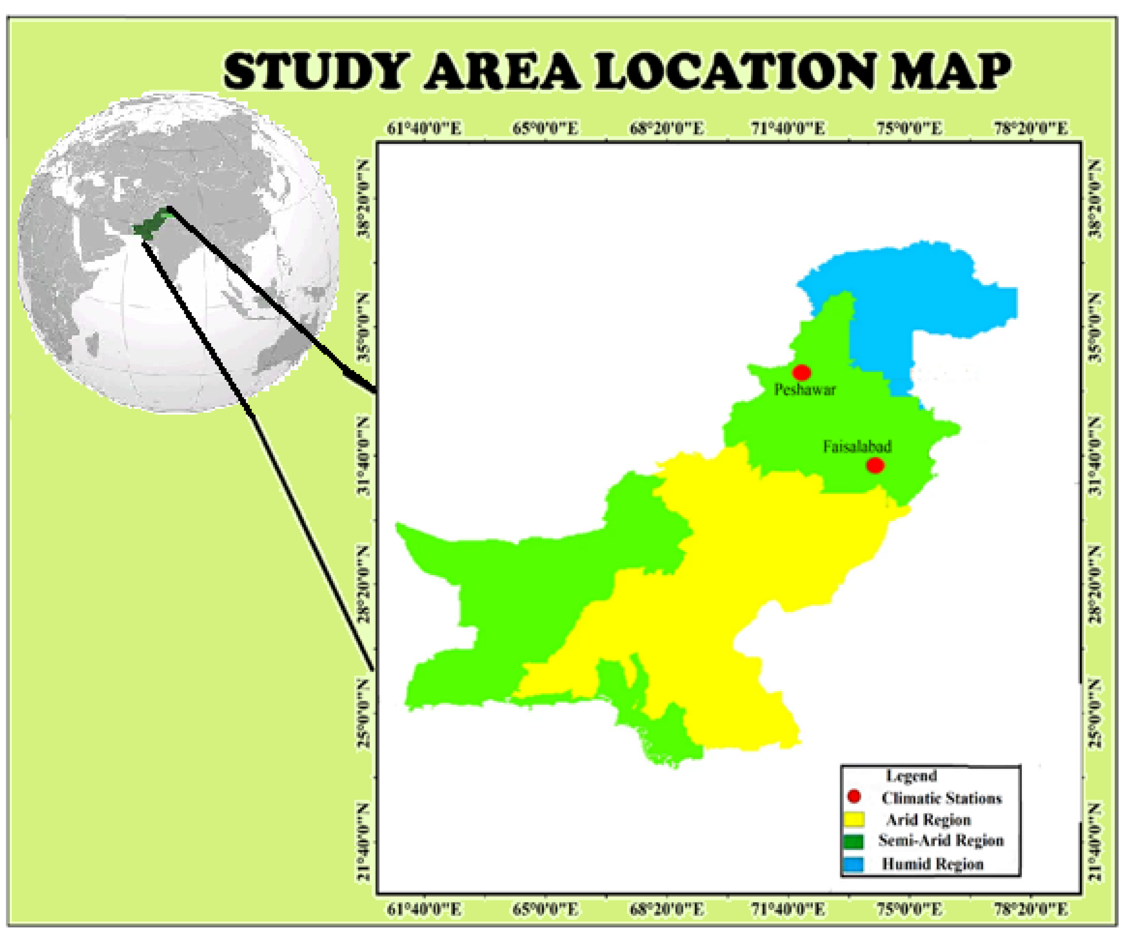
In this study, two semi-arid climatic stations are selected from Pakistan, as shown in Figure 1. Both stations are selected due to their geological and economical importance. Both stations were identified as semi-arid regions based on the aridity index. Due to its industrial and agricultural product production, Faisalabad is the key economical city of Punjab province in Pakistan. Wheat is a major crop grown in this area. The area comprises alluvial loess soils with calcareous characteristics that make this region very productive. This station has a mean sea elevation of 184 m with coordinates of 31.41 longitude and 73.11 latitudes. This area faces hot summer weather with a maximum temperature of 45 °C.

In contrast, the mean minimum and maximum temperatures are observed as 27 and 39 °C, respectively. In the winter, the mean minimum and maximum temperatures are recorded as 6 and 17 °C. Peshawar is the second climatic station selected in this study. It is the capital’s most economically populated city of Khyber Pakhtunkhwa province, with a population of 4 million. This station is situated at a mean sea elevation of 331 m with coordinates of 34.01 longitudes and 71.54 latitudes. This region has hot summer weather with mild winter. The mean annual rainfall is 400 mm in the region, with a higher rainfall ratio in the winter than summer. In summer, during the hottest month of July, maximum and minimum temperatures exceed 40 °C and 25 °C whereas, during the coldest month of December, the mean maximum and minimum temperatures are observed as 18.3 °C and 4 °C. For this study, minimum and maximum temperature data are collected from Pakistan meteorological department for the duration 1988 to 2015. Temperature data are easily available even in developing countries. Therefore, only temperature-based inputs with extraterrestrial radiation are used in this study. Extraterrestrial radiation is computed based on the Julian date and does not require any climatic data. For better data visualization, three training testing data partitions are adopted, such as 50–50%, 60–40%, and 75–25%. A brief statistical summary of both stations’ used data is summarized in

Table 1. The statistical parameters of the applied data.

	Tmin	Tmax	ET0	Ra
Faisalabad Station
Min.	3.25	16.15	1.07	18.83
Max.	28.8	42.2	10.53	41.34
Mean	17.5	31.1	4.71	31.05
Skewness	−0.241	−0.403	0.105	−0.181
Std. dev.	8.326	7.324	2.444	8.051
Peshawar Station
Min.	−1.45	15.95	1.41	17.23
Max.	26.7	40.5	10.04	41.58
Mean	16.5	29.6	5.36	30.25
Skewness	−0.176	−0.344	0.267	−0.147
Std. dev.	7.936	6.824	2.127	8.697

.

3. Methods

In this investigation, two new bio-inspired optimizers, the artificial hummingbird algorithm (AHA) and quantum-based avian navigation optimizer algorithm (QANA), are utilized for tuning RVFL and RVM methods in modeling ET₀. These algorithms were developed using knowledge of hummingbirds’ sophisticated foraging techniques and unique flight abilities. The implemented methods are described in the next sections.

3.1. Random Vector Functional Link Networks (RVFL)

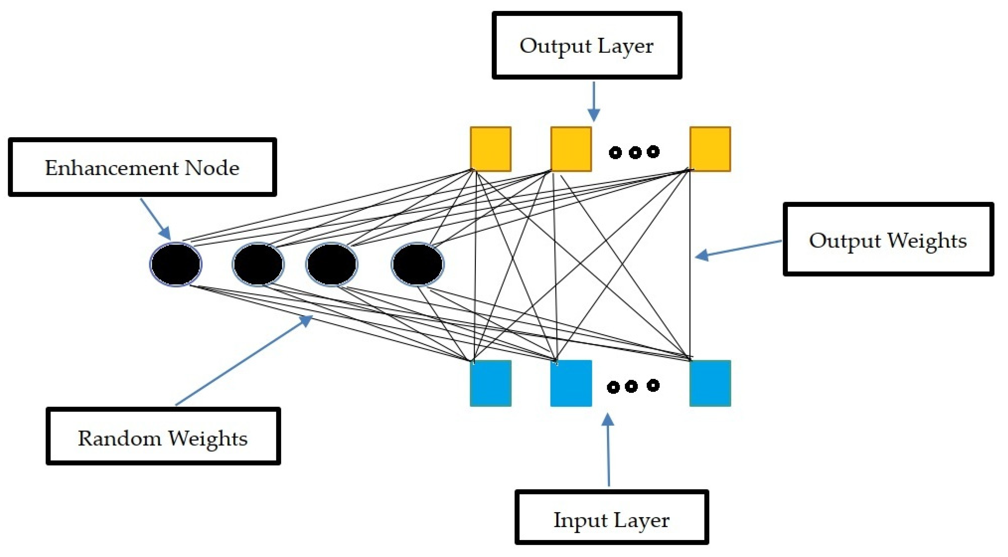
The Random Vector Functional Link (RVFL) networks transform the input pattern nonlinearly before being fed into the network’s input layer, creating an improved pattern [29,30]. A connection between the input and output layers is present in the RVFL, a form of Single Layer Feedforward Neural Network (SLFNN), as depicted in Figure 2.

The over-fitting issue, which is prevalent in traditional SLFNN, is avoided by this link. To induce an anticipated function, a functional link’s main goal is to try to expand a feature space. The aim variable, y_i, is obtained by the RVFL from the Ns sample data (X), which is represented as a pair (x_i, y_i). After that, the middle (hidden) nodes process the input data. The nodes of enhancement are these middle nodes. The output of every middle node is determined as follows Equation (1):

$$O_j\left({\alpha }_j{x}_i+{\beta }_j\right)=\frac{1}{1+e^{\left({\alpha }_j{x}_i+{\beta }_j\right)}} {\alpha }_jϵ\left[-S, S\right], {\beta }_jϵ\left[0, S\right]$$

(1)

where the weights between the enhancement (middle) nodes and the input layer nodes are denoted by ${\beta }_j$, and the bias is denoted by ${\alpha }_j$. During the optimization process, S, the scale factor, is assessed. The formula below computes the outcomes of RVFL:

$$Z=FW · WϵR^{n+p} · F=\left[F_1,F_2\right]$$

(2)

where W denotes the output weight, and F denotes a matrix made up of the intermediate layer’s F₂ result and the input sample F₁:

$$F_1=\left[\begin{array}{ccc}{x}_{1,1}& \cdots & x_{1,n}\\ ⋮& \ddots & ⋮\\ x_{N,1}& \cdots & x_{N,n}\end{array}\right] \mathrm{and} F_2=\left[\begin{array}{ccc}O\left({\alpha }_1{x}_1+{\beta }_1\right)& \cdots & O\left({\alpha }_p{x}_1+{\beta }_p\right)\\ ⋮& \ddots & ⋮\\ O\left({\alpha }_1{x}_N+{\beta }_1\right)& \cdots & O\left({\alpha }_p{x}_N+{\beta }_p\right)\end{array}\right]$$

(3)

The following equations, which, respectively, represent the Moore-Penrose pseudo-inverse and ridge regression, are used to update the output weight after the mentioned Equations (4) and (5):

$$W=F^{+\varphi \varphi }Z$$

(4)

$$W={\left(F^{T}F+\frac{1}{C}\right)}^{-1}{F}^{T}Z$$

(5)

where + is the Moore-Penrose pseudo-inverse and C is a trading-off parameter. An initial population of decision variables, called a “string”, is first randomly generated. The “fitness” of the population search string is then evaluated by considering the constraints and the objective function. Then, the ordered strings are linearly mapped to a fitness value ranking: highest and lowest mating probability. There is a mating pool at this stage, and the selected thread is assigned a mating partner.

3.2. Relevance Vector Machine (RVM)

As a special case of a sparse kernel model with an extended linear model with the same functional form as a support vector machine, RVM indicates a Bayesian approach to the model (SVM). It differs from SVM because the solution offers a probabilistic interpretation of the results [31,32]. By creating models with a structure and parameterization procedure that are both relevant to the information content of the data, RVM avoids complexity.

In the previously presented optimization process, the sparse Bayesian learning algorithm is critical to the RVM, obtained by the likelihood function and prior knowledge. In order to predict the function of y(x) at some random point x given a set of (usually noisy) measurements of the function t = (t₁,…, t_N) at certain training points x = (x₁,……, x_N), RVM begins with the notion of linear models:

$$t_i=y\left(x_i\right)+{\epsilon }_{i }$$

(6)

where ${\epsilon }_i$ represents the measurement’s noise component, which has a mean of 0 and a variation of ${\sigma }^2$. According to the premise of a linear model, the unknown function y(x) is a linear amalgamation of certain recognized basis functions ${\varphi }_i=\left(x\right)$, i.e., Equation (7):

$$y\left(x\right)={{\displaystyle \sum }}_{i=1}^M{w}_i{\varphi }_i\left(x\right)$$

(7)

where w = (w_i,…, w_M) is a vector consisting of the linear combination weights.

Equation (6) can then be written in vector form as follows:

$$t=\varphi w+\epsilon$$

(8)

If $\varphi$ is a N × M design matrix, the values of the basis function ${\varphi }_I\left(X\right)$ at each training points are produced in the ith column, and $\epsilon =\left({\epsilon }_1\dots \dots {\epsilon }_N\right)$ is the noise vector.

RVM begins with a collection of input data ${(X_n)}_{n=1}^N$ and their associated target vector ${(t_n)}_{n=1}^N$, as a supervised learning method. This “training” set’s objective is to create a model of the target vector’s dependence on the inputs to accurately forecast t for a value of x that has never been seen before. The prediction is estimated in the context of RVM based on a function of the form (Equation (9)):

$$y\left(x\right)={{\displaystyle \sum }}_{i=1}^N{w}_{i}K\left(x·x_i\right)+w_0$$

(9)

where the weight vectors w = (w₁, w₂, …, w_N), the bias w₀, and the kernel function K (x, xi) are all present.

We use the conventional formulation and assume p(t|x) is Gaussian N(t|y(x), ${\sigma }^2$). given a data set of input-target pairs ${(X_n·t_n)}_{n=1}^N$. The expression y(x), as defined in Equation (6), models the mean of this distribution for a given x. The dataset’s likelihood can be expressed as Equation (10):

$$p\left(t|w,{\sigma }^2\right)={\left(2\pi {\sigma }^2\right)}^{-N/2}exp\left\{-\frac{1}{2{\sigma }^2} t-\varphi w^2\right\}$$

(10)

where t = (t₁, …., t_N), w = (w₀,…, w_N) and $\Phi$ is the N*(N+1) “design” matrix with ${\Phi }_{nm}=K\left(x_n·x_{m-1}\right)$ and ${\Phi }_{n1}=1$. Overfitting frequently occurs when w and ${\sigma }^2$ in Equation (6) are estimated with maximum probability. Tipping [33], therefore, advised imposing previous constraints on the parameters by making the likelihood or error function more complex. The learning process’ capacity for generalization is governed by this a priori knowledge. New higher-level parameters are typically used to constrain an explicit zero-mean Gaussian prior probability distribution over the weights (Equation (11)):

$$p(w\left|\alpha )={{\displaystyle \prod }}_{i=0}^{N}N(w_i\left|0,{\alpha }_i^{-1})\right.\right.$$

(11)

Each weight can depart from zero by a vector of (N*1) hyperparameters called [6]. Given the above non-informative prior distributions, Bayes’ rule could be used to determine the posterior overall unknowns (Equation (12)).

$$p\left(w,\alpha ,{\sigma }^2\left|t\right.\right)=\frac{p(t\left|w,\alpha ,{\sigma }^2)p\left(w,\alpha ,\sigma \right)\right.}{\int p(t\left|w,\alpha ,{\sigma }^2)p\left(w,\alpha ,{\sigma }^2\right)dwd\alpha d{\sigma }^2\right.}$$

(12)

However, since we are unable to carry out the normalizing integral, $p\left(t\right)=\int p(\frac{t}{w},\alpha ,{\sigma }^2)p\left(w,\alpha ,{\sigma }^2\right)dw d\alpha d{\sigma }^2$, we calculate the posterior solution in Equation (13) directly. Instead, we break down the back as Equation (13):

$$p(w,\alpha ,{\sigma }^2\left|B)=p(w\left|t,\alpha ,{\sigma }^2)p\left(\alpha ,{\sigma }^2\left|t\right.\right)\right.\right.$$

(13)

to make the solution easier. Given by is the posterior distribution of weights (Equation (14)).

$$p(w\left|t,\alpha ,{\sigma }^2)=\frac{p(t\left|w,{\sigma }^2)p\left(w,\alpha \right)\right.}{p(t\left|\alpha ,{\sigma }^2)\right.}\right.$$

(14)

Bayes’ rule is then used to determine the posterior over the weights (Equation (15)):

$$p(w\left|t,\alpha ,{\sigma }^2)=2{\pi }^{-\left(N+1\right)/2}{\left|\Sigma \right|}^{-1/2}exp\left\{-\frac{1}{2}{\left(w-\mu \right)}^T{\Sigma }^{-1}\left(W-\mu \right)\right\}\right.$$

(15)

There is an analytical answer to Equation (18) where the mean and posterior covariance are the following:

$$\Sigma ={\left({\varphi }^{T}B\varphi +A\right)}^{-1}$$

(16)

$$\mu =\Sigma {\varphi }^{T}Bt$$

(17)

where we have defined $A={\alpha }_o,{\alpha }_1\dots \dots {\alpha }_N)$ and $B={\sigma }^{-2}{1}_N.$ is also treated as a hyperparameter, which maybe estimated from the data.

As a result, machine learning evolved into a search for the posterior-most probable hyperparameters. The marginal likelihood for the hyperparameters is then calculated by integrating the weights, and predictions are then created for a new set of data:

$$p(t\left|\alpha ,{\sigma }^2)=\int p(t\left|w,{\sigma }^2)p(w\left|\alpha )\mathrm{dw}={\left(2\pi \right)}^{-N/2}\left|B^{-1}+\varphi A^{-1}{\varphi }^T\left|-1/2\right.\exp \left\{-\frac{1}{2}{t}^T{\left(B^{-1}+\varphi A^{-1}{\varphi }^T\right)}^{-1}t\right\}\right.\right.\right.\right.$$

(18)

As a machine learning method, the RVM-based tool wear prediction model also includes two important processes model construction and performance evaluation. The inputs of the RVM in the two processes are feature vectors composed of machining parameters and features obtained from monitoring signals [34].

3.3. Artificial Hummingbird Algorithm (AHA)

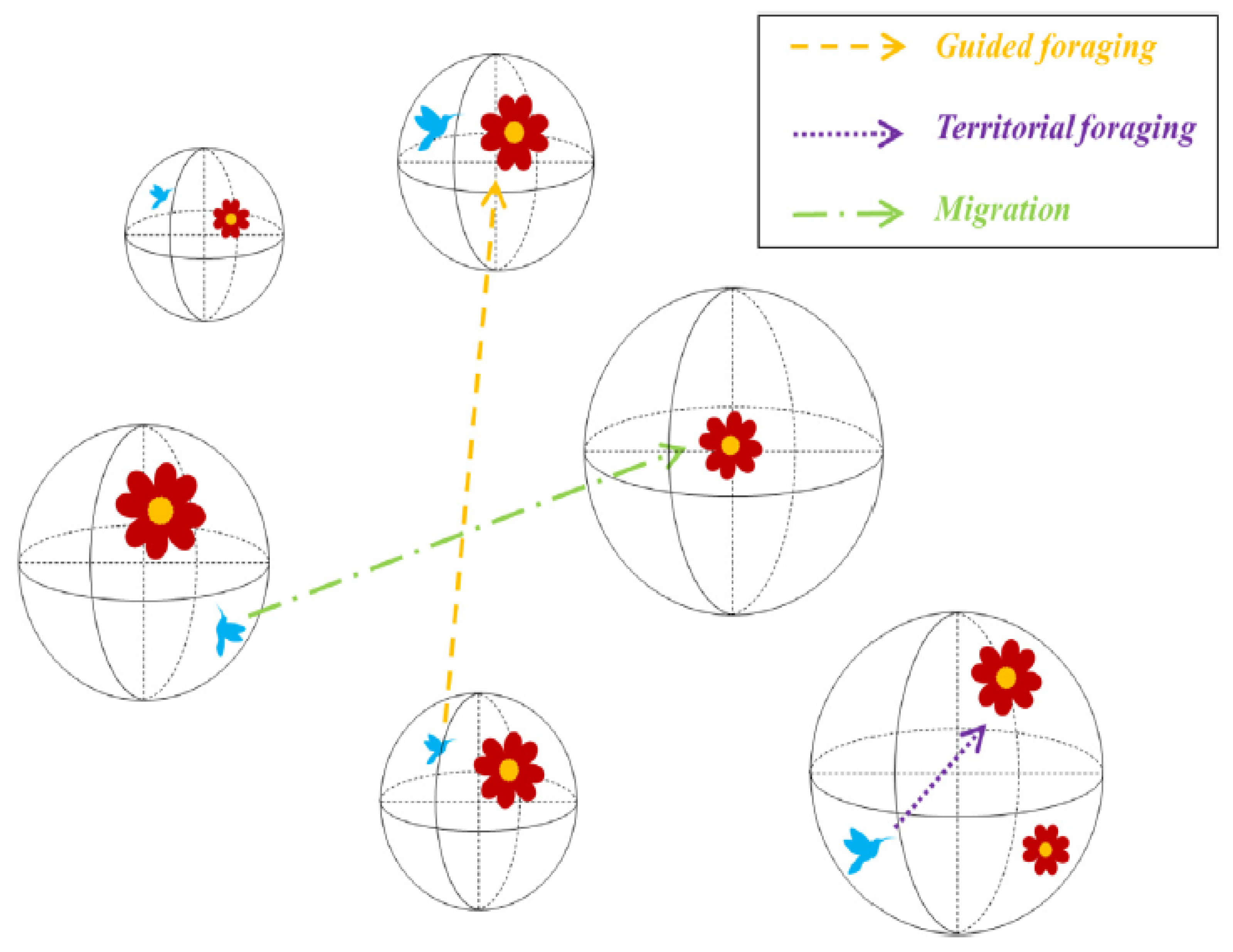
Although AHA is a meta-heuristic, it differs greatly from other existing algorithms. The most notable difference between AHA and the others is its unique biological basis. AHA was founded on three foraging techniques and three flight maneuvers used by hummingbirds in the wild. Another important distinction is between exploration and exploitation. The territorial foraging strategy in AHA fosters exploitation, whereas the migration foraging strategy ensures search space exploration.

In contrast, the guided foraging method prioritizes exploration over exploitation. The third difference between AHA and current algorithms is its unique memory update mechanism. Each hummingbird must know when the others last visited to choose its preferred food source. This information is saved in a visiting table. When the factors above are considered, AHA and existing algorithms differ dramatically. Good literature attempts to model the search behaviors of hummingbirds using Levy flight and the best individuals Zhang et al. [35]. However, the proposed optimizer in this work attempts to mimic the search behaviors of hummingbirds using three foraging strategies and their exceptional memory and impressive flight abilities [36,37]. AHA imitates three flying patterns—axial, diagonal, and omnidirectional—and three different search tactics—guided foraging, territorial foraging, and migratory. In addition, a critical component known as the visit table is included to imitate how hummingbirds use their memory to identify and select food sources (see Figure 3).

This work proposes an artificial hummingbird algorithm (AHA), a product bio-inspired optimization method, to address optimization challenges. The AHA algorithm simulates hummingbirds’ unique flight talents and smart foraging strategies in the wild.

In this piece, we looked through AHA, an optimization method that takes some cues from the ingenuity of hummingbirds. Following is an outline of the three fundamental tenets of AHA.

What we eat: In reality, a hummingbird chooses an appropriate food source from a set by evaluating its properties, such as the nectar quality and content of individual flowers, the nectar-refilling rate, and the most recent time of visit. A food source in AHA is a solution vector, and the rate at which its nectar is replenished is represented by its function fitness value; this assumption is made for simplicity. The fitness benefits of a food source include a faster rate of nectar replenishment.

The frequency with which different hummingbirds return to the same food source is recorded in a “visit table,” which also keeps track of how long it has been since the same hummingbird last visited that source. Suppose a hummingbird has a choice between two food sources. In that case, it will preferentially visit the one that receives the most visits overall.

3.4. Quantum-Based Avian Navigation Optimizer Algorithm (QANA)

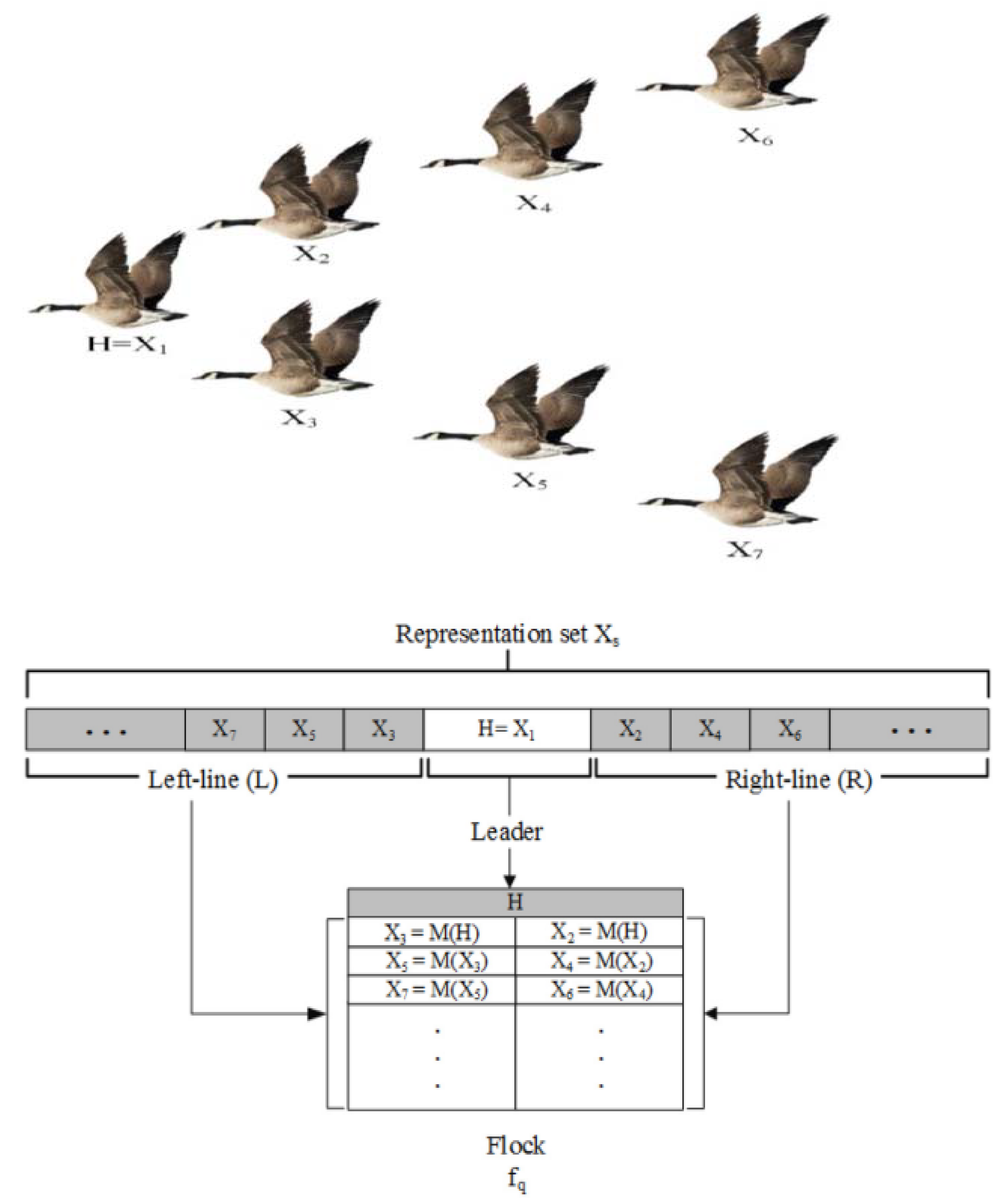
In order to solve problems requiring global optimization, differential evolution has become a common and effective method. However, when the problem’s dimension expands, the solution’s efficacy and scalability decline. As a result, this research focuses on developing a brand-new DE approach called the quantum-based avian navigation optimizer algorithm (QANA), which was prompted by the extraordinarily exact navigation of migrating birds along long-distance aerial routes. Using the proposed self-adaptive quantum orientation and quantum-based navigation, which incorporated the two mutation procedures DE/quantum/I and DE/quantum/II, the QANA distributes the population by splitting it into multiple flocks to explore the search space successfully. Except for the first iteration, each flock is randomly assigned to one of the quantum mutations approaches using a newly created success-based population distribution (SPD) strategy. In the meantime, a novel communication topology known as V-echelon is utilized to distribute the information flow among the population. In addition to providing a qubit-crossover operator for developing advanced search agents, we also provide both long-term and short-term memory for storing data necessary for performing a partial landscape analysis. The suggested QANA’s efficacy and scalability were extensively evaluated using the benchmark functions CEC 2018 and CEC 2013 as LSGO problems [38].

A robust and scalable DE algorithm, the quantum-based avian navigation optimizer algorithm (QANA), is offered as a solution to LSGO problems. The QANA was inspired by the extraordinary feats of the migrating birds, which use a quantum-based avian navigator and communication topology to easily fly great distances [2,7]. The following are some of how we helped to create this robust QANA algorithm:

To allocate flocks effectively, we provide the success-based population distribution (SPD) policy that exploits mutational approaches.

Keep things interesting by including both long-term and short-term memory.

Information sharing and management are best accomplished by implementing a V-echelon topology, as recommended below.

Designing a couple of novel mutation strategies for quantum-based positioning systems.

A qubit-crossover operator can help search agents obtain better results.

3.5. Proposed Optimized RVM and RVFL Models

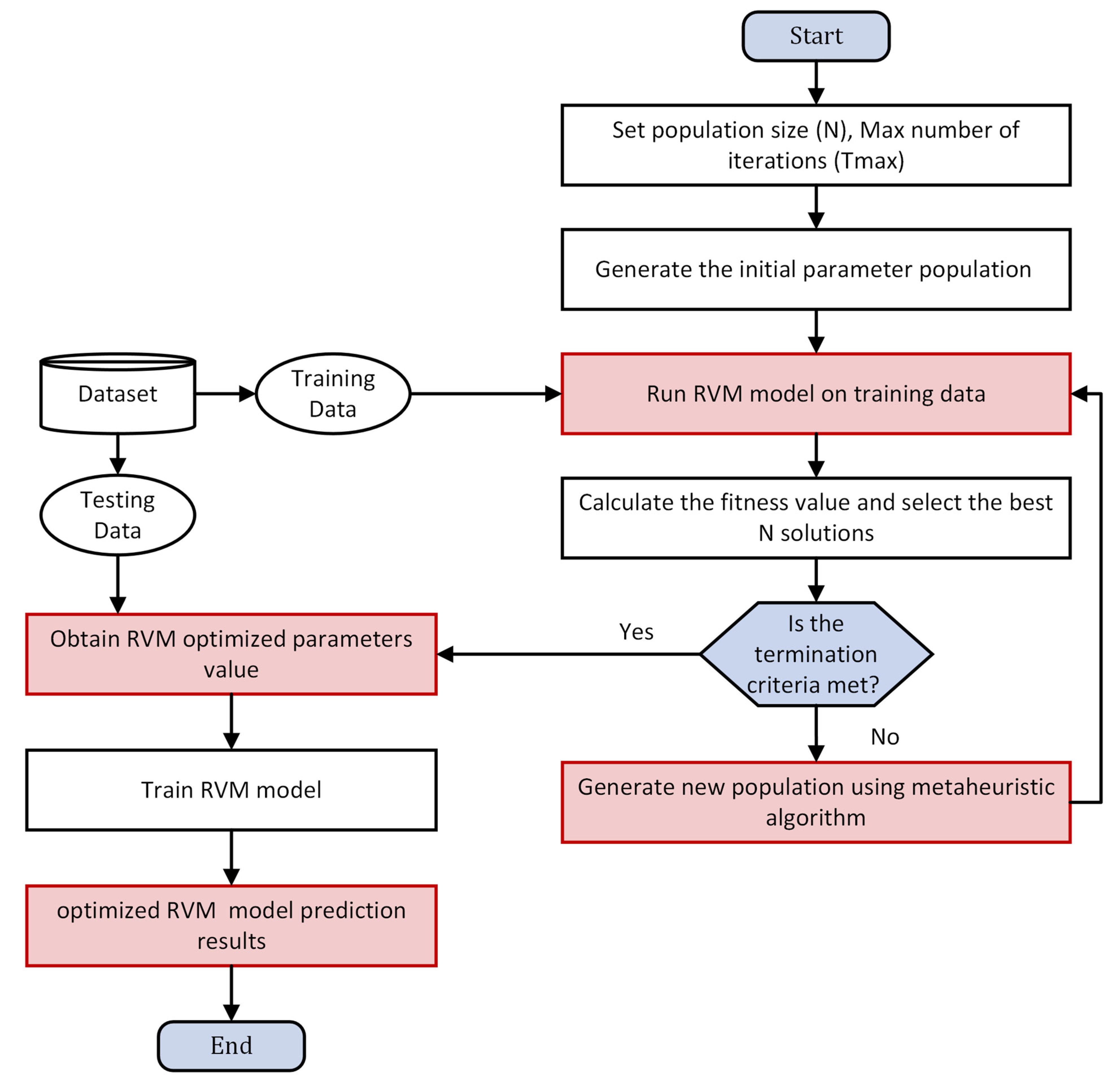
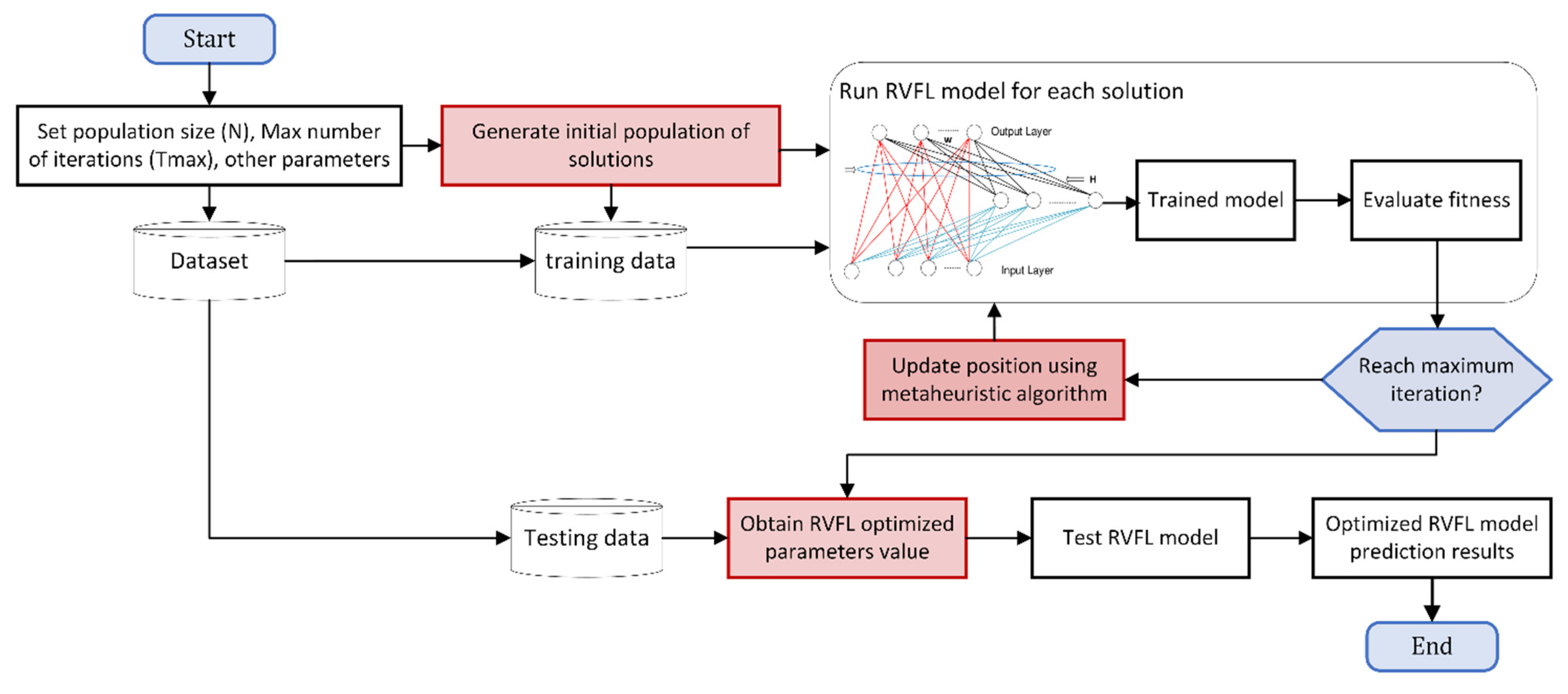
The performance of RVM and RVFL depends on selecting appropriate model hyper-parameters. In order to improve the performance of RVM and RVFL models, they were integrated with two most recent metaheuristic algorithms (AHA and QANA). Gaussian kernel function was adopted for the RVM model. The main RVFL parameters are the activation function, bias, and hidden node number. In the presented study, 200 hidden neurons were used, with bias at the output. The activation function was radial in RVFL. The main steps of the optimized RVM and RVFL models are illustrated in Figure 4 and Figure 5, respectively.

Optimizing RVM and RVFL models with AHA and QANA was started by normalizing the datasets into the range of 0–1. Data were split into 70% (training) and 30% (testing). RMSE was used as a fitness function, and the training process was repeated till the maximum iteration was met. The quality of the optimized RVM and RVFL models was assessed utilizing 30% of the samples (testing data) with evaluation metrics to compute the target output.

3.6. Assessment of the Developed Methods and Parameters

The implemented models in this study were compared with single versions and assessed based on the following criteria:

$$RMSE:Root Mean Square Error=\sqrt{\frac{1}{N}{{\displaystyle \sum }}_{i=1}^N{[{(Y_0)}_i-{(Y_C)}_i]}^2}$$

(19)

$$MAE:Mean Absolute Error=\frac{1}{N}{{\displaystyle \sum }}_{i=1}^N|{(Y_0)}_i-{(Y_C)}_i|$$

(20)

$$R^2:Determination Coefficient={\left[\frac{{{\displaystyle \sum }}_{t=1}^N\left(Y_o-\overline{Y_o}\right)\left(Y_c-\overline{Y_c}\right)}{\sqrt{{{\displaystyle \sum }}_{t=1}^N{(Y_o-\overline{Y_o})}^2{(Y_c-\overline{Y_c})}^2}}\right]}^2$$

(21)

$$NSE:Nash-Sutcliffe Efficiency=1-\frac{{{\displaystyle \sum }}_{i=1}^N{[{(Y_0)}_i-{(Y_c)}_i]}^2}{{{\displaystyle \sum }}_{i=1}^N{[{(Y_0)}_i-{\overline{Y}}_0]}^2},-\infty <NSE\le 1$$

(22)

where $Y_c$ is calculated ET₀, $Y_o$ is observed ET₀, ${\overline{Y}}_o$ is mean FAO PM 56 ET₀ $N$ is a number of data.

Table 2. Parameter settings for all algorithms.

Algorithm	Parameter	Value
AHA	Migration coefficient	2n
	r	∈ [0,1]
QANA	The number of flocks (𝑘)	10
	K’	9
	K’	50
Common Settings	Population	30
	Number of iterations	100
	Number of runs for each Algorithm	30

gives brief information related to the setting parameters of the used MH algorithms. For each model, 30 populations were set, and 1000 iterations were employed. The algorithms were run 30 times to reach the final solution.

4. Results

The study investigates the viability of two machine learning methods, RVFL and RVM, improved by two metaheuristics (MH) algorithms, AHA and QANA, in estimating ET₀ using limited input data (Tmin, Tmax, and Ra). The models were assessed using three data split scenarios (50–50%, 60–40%, and 75–25%), and the results were tabulated for the best-split scenario of each method. Training and testing results of the single RVFL models in estimating ET₀ of Faisalabad Station are summed up in

Table 3. The results of the RFVL-based models for Faisalabad Station using the best training-test partition (75–25% scenario).

Inputs Combinations	Training Period				Test Period
	RMSE	MAE	R2	NSE	RMSE	MAE	R2	NSE
RFVL
(i) Tmin, Tmax	0.9049	0.7135	0.8012	0.8012	0.9181	0.7261	0.7987	0.7940
(ii) Tmin, Ra	0.7069	0.5387	0.9156	0.9128	0.7173	0.5458	0.9081	0.9058
(iii) Tmax, Ra	0.6849	0.5206	0.9240	0.9210	0.6875	0.5234	0.9180	0.9177
(iv) Tmin, Tmax, Ra	0.6919	0.5314	0.9216	0.9210	0.6983	0.5361	0.9166	0.9144
(v) Tmin, Tmax, Ra, MN	0.6825	0.5183	0.9228	0.9203	0.6866	0.5222	0.9221	0.9186
Mean	0.7342	0.5645	0.8970	0.8953	0.7416	0.5707	0.8927	0.8901
RFVL-AHA
(i) Tmin, Tmax	0.8893	0.6939	0.8116	0.8114	0.9122	0.7140	0.8056	0.8021
(ii) Tmin, Ra	0.6375	0.4868	0.9492	0.9473	0.6447	0.4901	0.9469	0.9456
(iii) Tmax, Ra	0.6182	0.4569	0.9583	0.9567	0.6235	0.4625	0.9558	0.9543
(iv) Tmin, Tmax, Ra	0.6081	0.4524	0.9621	0.9596	0.6164	0.4599	0.9587	0.9572
(v) Tmin, Tmax, Ra, MN	0.6059	0.4507	0.9637	0.9605	0.6158	0.4562	0.9591	0.9580
Mean	0.6718	0.5081	0.9290	0.9271	0.6825	0.5165	0.9252	0.9234
RFVL-QANA
(i) Tmin, Tmax	0.8565	0.6715	0.8340	0.8321	0.9082	0.7051	0.8058	0.8055
(ii) Tmin, Ra	0.6329	0.4816	0.9483	0.9462	0.6466	0.4861	0.9451	0.9448
(iii) Tmax, Ra	0.6034	0.4517	0.9625	0.9617	0.6082	0.4553	0.9608	0.9604
(iv) Tmin, Tmax, Ra	0.5958	0.4452	0.9649	0.9632	0.6068	0.4471	0.9625	0.9616
(v) Tmin, Tmax, Ra, MN	0.6028	0.4459	0.9638	0.9617	0.6079	0.4491	0.9616	0.9609
Mean	0.6583	0.4992	0.9347	0.9330	0.6755	0.5085	0.9272	0.9266

. As seen from the table, five input combinations were considered. The fifth combination considers the periodicity component (MN, month number of the output). It is apparent from Table 3 that the RVFL model with full inputs (Tmin, Tmax, Ra, and MN) offers better estimations compared to other input combinations. Table 3 also provides the outcomes of the improved RVFL models, RVFL-AHA and RVFL-QANA, for the Faisalabad Station. It is visible from

Table 4. The results of the RVM-based models for Faisalabad Station using the best training-test partition (75–25% scenario).

Inputs Combinations	Training Period				Test Period
	RMSE	MAE	R2	NSE	RMSE	MAE	R2	NSE
RVM
(i) Tmin, Tmax	0.9042	0.7125	0.8074	0.8043	0.9115	0.7134	0.8061	0.8025
(ii) Tmin, Ra	0.6873	0.5397	0.9253	0.9242	0.6960	0.5414	0.9204	0.9200
(iii) Tmax, Ra	0.6827	0.5209	0.9279	0.9269	0.6854	0.5220	0.9259	0.9244
(iv) Tmin, Tmax, Ra	0.6809	0.5204	0.9283	0.9274	0.6826	0.5227	0.9269	0.9260
(v) Tmin, Tmax, Ra, MN	0.6695	0.5106	0.9324	0.9315	0.6734	0.5134	0.9307	0.9294
Mean	0.7249	0.5608	0.9043	0.9029	0.7298	0.5626	0.9020	0.9005
RVM-AHA
(i) Tmin, Tmax	0.8615	0.6672	0.8269	0.8257	0.9020	0.7139	0.8125	0.8087
(ii) Tmin, Ra	0.6396	0.4835	0.9503	0.9486	0.6437	0.4890	0.9472	0.9460
(iii) Tmax, Ra	0.5798	0.4348	0.9681	0.9681	0.6229	0.4594	0.9548	0.9546
(iv) Tmin, Tmax, Ra	0.5546	0.4149	0.9775	0.9775	0.6068	0.4487	0.9621	0.9610
(v) Tmin, Tmax, Ra, MN	0.5460	0.4062	0.9805	0.9805	0.6047	0.4462	0.9626	0.9617
Mean	0.6363	0.4813	0.9407	0.9401	0.6760	0.5114	0.9278	0.9264
RVM-QANA
(i) Tmin, Tmax	0.8067	0.6214	0.8560	0.8560	0.8900	0.7048	0.8164	0.8163
(ii) Tmin, Ra	0.6119	0.4492	0.9569	0.9569	0.6413	0.4824	0.9484	0.9470
(iii) Tmax, Ra	0.6076	0.4583	0.9612	0.9603	0.6143	0.4547	0.9587	0.9580
(iv) Tmin, Tmax, Ra	0.5766	0.4262	0.9706	0.9706	0.6070	0.4542	0.9616	0.9609
(v) Tmin, Tmax, Ra, MN	0.5604	0.4141	0.9765	0.9765	0.6062	0.4438	0.9639	0.9622
Mean	0.6326	0.4738	0.9442	0.9441	0.6718	0.5080	0.9298	0.9289

that the RVFL-AHA with input combination (v) acts as the best model. In the case of RVFL-QANA, the models with input combinations (iii) and (iv) perform the best in the estimation of ET₀, respectively.

It is clear from the RVFL-based models (see Table 3) that Tmax, Ra input is more effective on ET₀ than the Tmin, Ra. A comparison of the single RVFL and hybrid versions reveals that the hybrid models improve the accuracy of the single RVFL model in estimating ET₀.

The outcomes of the single and hybrid RVM models in estimating ET₀ of Faisalabad Station are reported in Table 4 for the best training-test scenario (75–25%). There is a marginal difference between the input combinations (iv) and (v). Adding MN into the inputs slightly improves the RVM accuracy.

It is clear from Table 4 enlisting the training and testing outcomes of the hybrid RVM models that for hybrid models, also periodicity slightly improves the models’ accuracy in estimating ET₀. Like RVM-based models, here also Tmax, Ra inputs seem more effective on ET₀ than the Tmin, Ra inputs. The last performance belongs to the models having Tmin and Tmax inputs. It is apparent from Table 4 that the RVM-AHA and RVM-QANA perform superior to the single RVM models as found for the RVFL-based models. It is visible from the single and hybrid RVFL and RVM models (Table 3 and Table 4) that importing Ra into the model inputs considerably improves the efficiency in estimating ET₀.

Training and testing results of RVFL-based models are provided in

Table 5. The results of the RFVL-based models for Peshawar Station using the best training-test partition (75–25% scenario).

Inputs Combinations	Training Period				Test Period
	RMSE	MAE	R2	NSE	RMSE	MAE	R2	NSE
RFVL
(i) Tmin, Tmax	0.7186	0.5687	0.8571	0.8571	0.8369	0.6786	0.8525	0.8303
(ii) Tmin, Ra	0.7392	0.5541	0.9220	0.9196	0.7554	0.6083	0.9136	0.9038
(iii) Tmax, Ra	0.6791	0.5034	0.9333	0.9333	0.7144	0.5371	0.9159	0.9098
(iv) Tmin, Tmax, Ra	0.6495	0.4879	0.9444	0.9441	0.6961	0.5452	0.9178	0.9128
(v) Tmin, Tmax, Ra, MN	0.6483	0.4861	0.9446	0.9444	0.6943	0.5360	0.9195	0.9141
Mean	0.6869	0.5200	0.9203	0.9197	0.7394	0.5810	0.9039	0.8942
RFVL-AHA
(i) Tmin, Tmax	0.6998	0.5617	0.8649	0.8645	0.7852	0.6376	0.8342	0.8366
(ii) Tmin, Ra	0.5047	0.4150	0.9531	0.9352	0.5342	0.4101	0.9524	0.9301
(iii) Tmax, Ra	0.4198	0.3594	0.9634	0.9467	0.4905	0.3828	0.9572	0.9447
(iv) Tmin, Tmax, Ra	0.4268	0.3360	0.9651	0.9543	0.4367	0.3617	0.9623	0.9502
(v) Tmin, Tmax, Ra, MN	0.3841	0.2876	0.9724	0.9635	0.3917	0.2904	0.9691	0.9567
Mean	0.4870	0.3919	0.9438	0.9328	0.5277	0.4165	0.9350	0.9237
RFVL-QANA
(i) Tmin, Tmax	0.6519	0.5101	0.8835	0.8824	0.7756	0.6052	0.8535	0.8413
(ii) Tmin, Ra	0.4895	0.3827	0.9564	0.9361	0.5016	0.3921	0.9543	0.9348
(iii) Tmax, Ra	0.3935	0.3060	0.9648	0.9526	0.4408	0.3451	0.9637	0.9514
(iv) Tmin, Tmax, Ra	0.3426	0.2690	0.9693	0.9671	0.3754	0.2935	0.9689	0.9632
(v) Tmin, Tmax, Ra, MN	0.3892	0.3022	0.9704	0.9581	0.4223	0.3435	0.9670	0.9541
Mean	0.4533	0.3540	0.9489	0.9393	0.5031	0.3959	0.9415	0.9290

for estimating ET₀ of Peshawar Station for the best training-test scenario. It is visible from the tables that the models with Tmax, Ra inputs perform superior to the models having inputs of Tmin, Ra. The models with Tmin, Tmax, Ra, and MN inputs outperform the other alternatives. In some cases, however, considering MN in inputs deteriorates the models’ accuracy in ET₀ estimation; for example, a 75–25% scenario of RVFL-QANA. It should be noted that the models with only temperature inputs (Tmin, Tmax) produce inferior ET₀ estimates in all cases and for all RVFL-based models.

The outcomes of single and hybrid RVM models are enlisted in

Table 6. The results of the RVM-based models for Peshawar Station using the best training-test partition (75–25% scenario).

Inputs Combinations	Training Period				Test Period
	RMSE	MAE	R2	NSE	RMSE	MAE	R2	NSE
RVM
(i) Tmin, Tmax	0.7157	0.5647	0.8584	0.8583	0.8346	0.6260	0.8092	0.7915
(ii) Tmin, Ra	0.6678	0.5502	0.9215	0.9136	0.6759	0.5900	0.9199	0.8929
(iii) Tmax, Ra	0.6410	0.4934	0.9363	0.9333	0.6578	0.5414	0.9216	0.9201
(iv) Tmin, Tmax, Ra	0.6100	0.4815	0.9328	0.9256	0.6435	0.5362	0.9289	0.9205
(v) Tmin, Tmax, Ra, MN	0.5951	0.4725	0.9461	0.9452	0.6436	0.5369	0.9297	0.9283
Mean	0.6459	0.5125	0.9190	0.9152	0.6911	0.5661	0.9019	0.8907
RVM-AHA
(i) Tmin, Tmax	0.7060	0.5649	0.8629	0.8621	0.7853	0.6096	0.8577	0.8466
(ii) Tmin, Ra	0.4567	0.3540	0.9499	0.9198	0.5385	0.4169	0.9474	0.9346
(iii) Tmax, Ra	0.4284	0.3501	0.9620	0.9418	0.4338	0.3612	0.9575	0.9410
(iv) Tmin, Tmax, Ra	0.4110	0.3409	0.9662	0.9560	0.4258	0.3529	0.9650	0.9534
(v) Tmin, Tmax, Ra, MN	0.3618	0.2988	0.9695	0.9594	0.3688	0.3009	0.9665	0.9573
Mean	0.4728	0.3817	0.9421	0.9278	0.5104	0.4083	0.9388	0.9266
RVM-QANA
(i) Tmin, Tmax	0.5643	0.4390	0.9119	0.9119	0.7823	0.6087	0.8537	0.8480
(ii) Tmin, Ra	0.4104	0.3208	0.9618	0.9534	0.4682	0.3880	0.9548	0.9312
(iii) Tmax, Ra	0.3659	0.2810	0.9630	0.9630	0.3999	0.3185	0.9623	0.9498
(iv) Tmin, Tmax, Ra	0.3088	0.2328	0.9736	0.9736	0.4347	0.3616	0.9685	0.9407
(v) Tmin, Tmax, Ra, MN	0.3132	0.2452	0.9729	0.9729	0.3252	0.2696	0.9705	0.9668
Mean	0.3925	0.3038	0.9566	0.9550	0.4821	0.3893	0.9420	0.9273

for estimating ET₀ in Peshawar Station for the best training-test scenario (75–25%). It is clear from the table that the models with full inputs (input combination (v)) generally act as the best in estimating ET₀. Here also, Tmax, Ra combination provides the worst outcomes for single and hybrid RVM models. It is understood from the table that tuning RVM parameters with AHA and QANA methods improve its accuracy in estimating ET₀ using limited climatic inputs. A comparison of RVM and RVFL models reveals that the RVM-based models generally act better than the RVFL-based models concerning mean statistics of RMSE, MAE, R², and NSE.

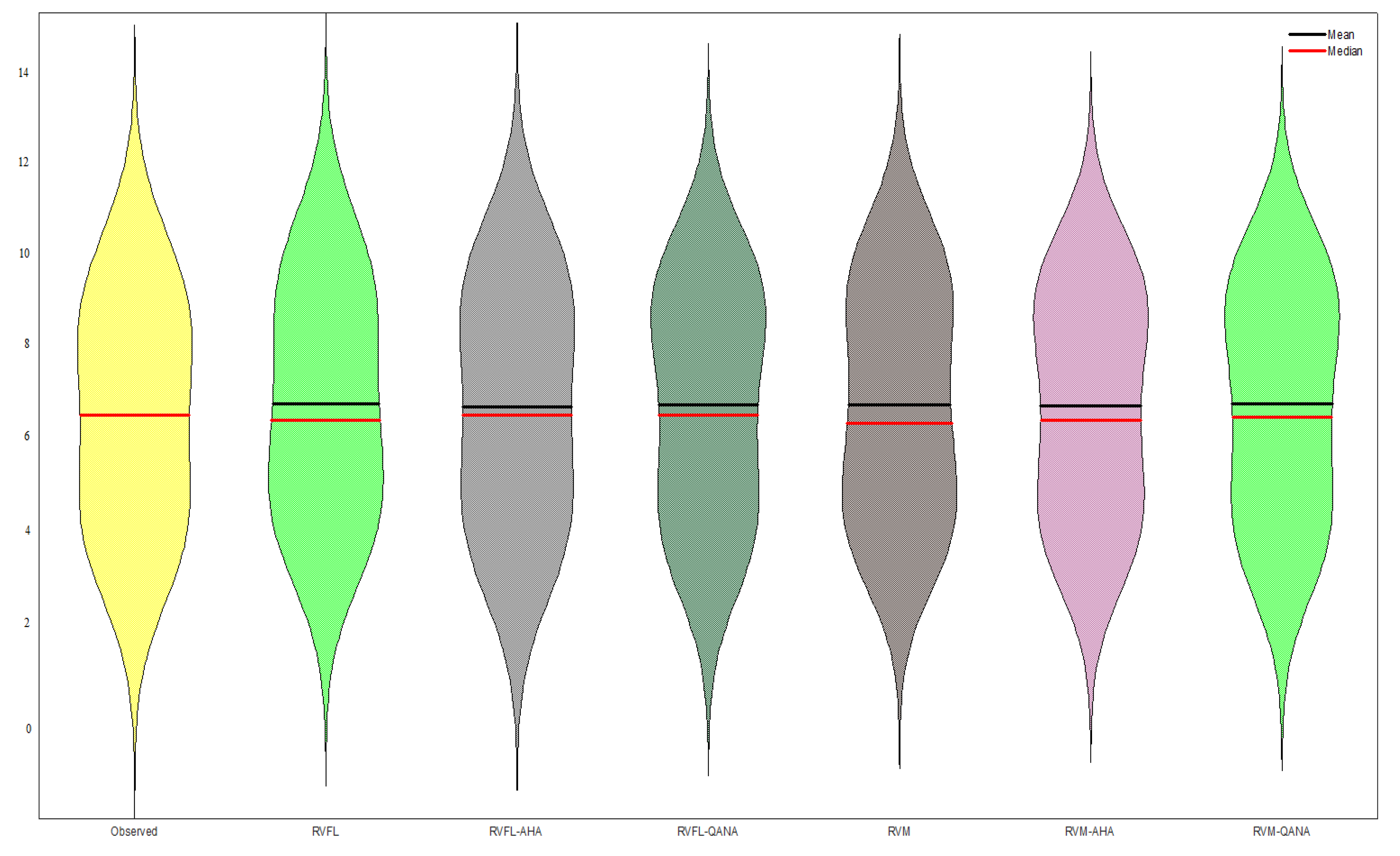
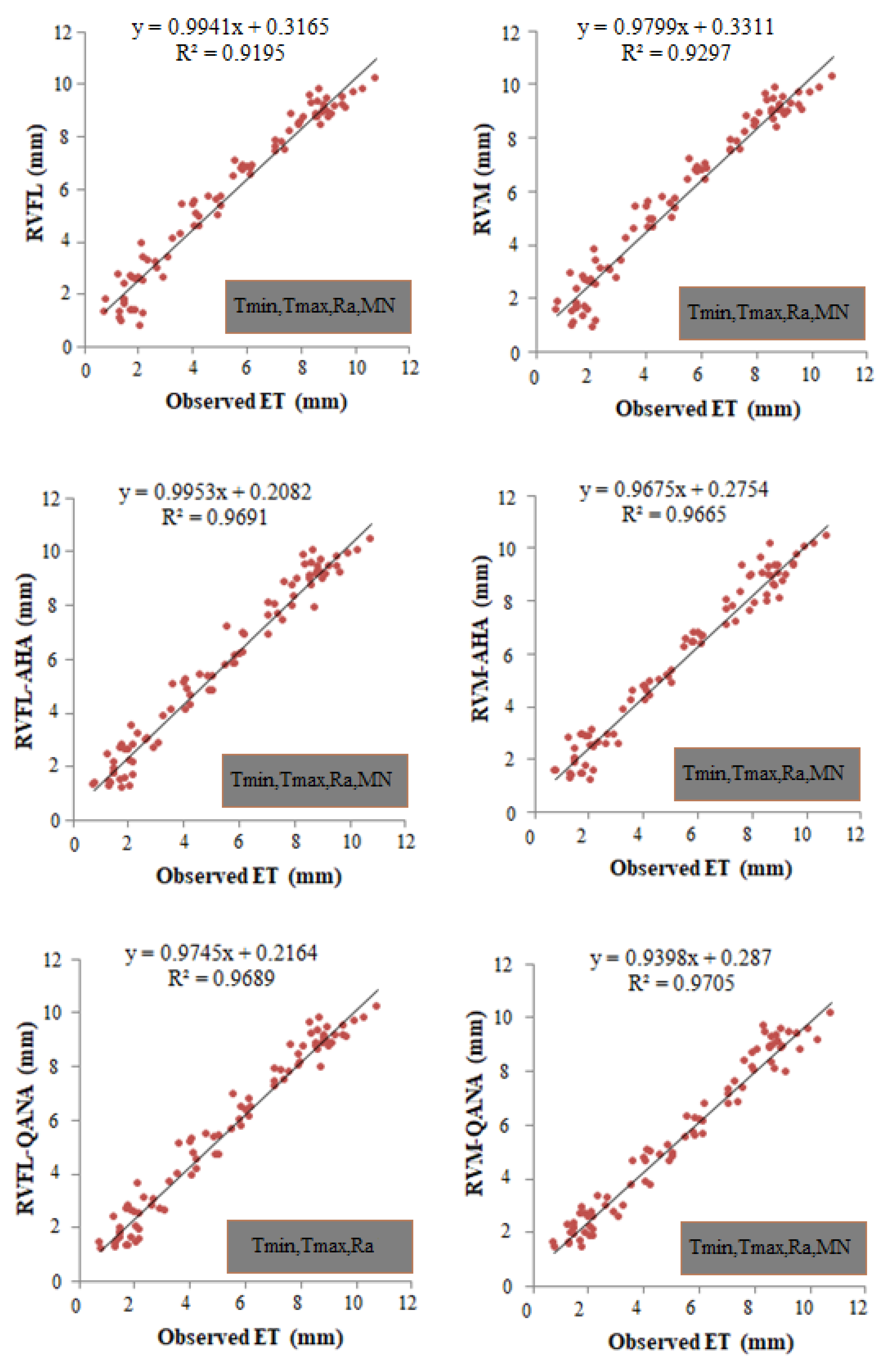
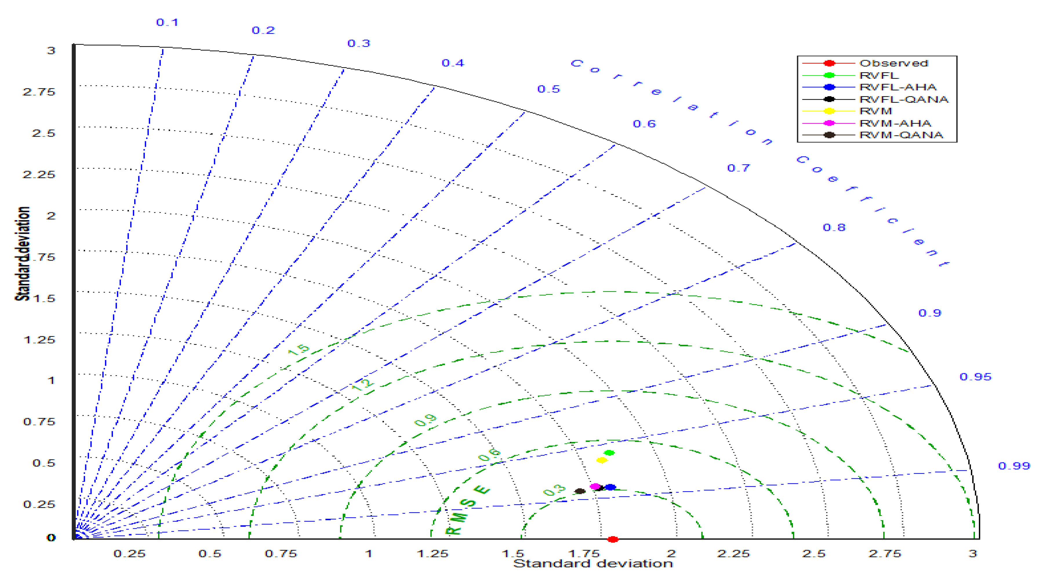
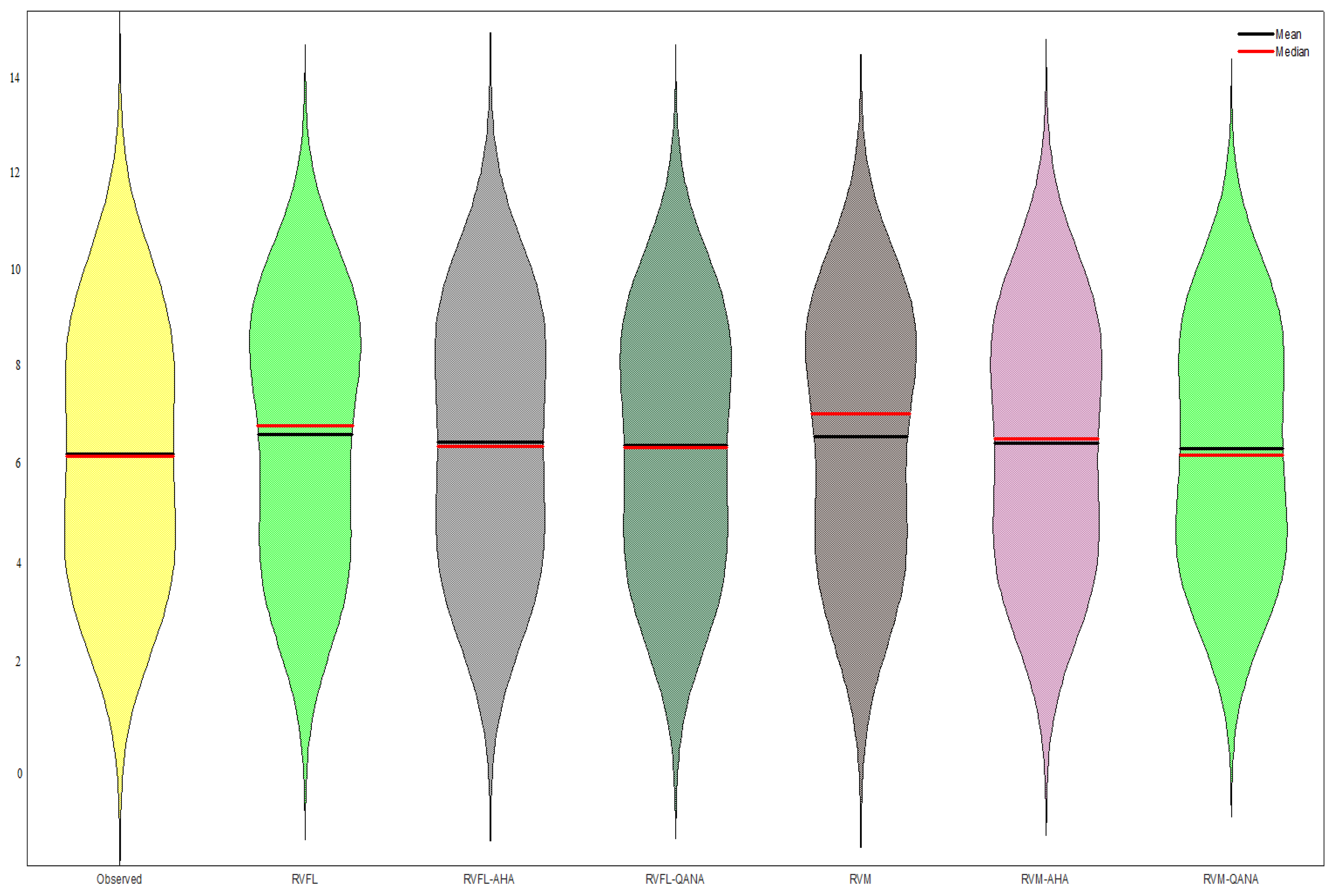
The scatterplots in Figure 6 compare the optimal RVFL and RVM-based models for the test period of Faisalabad Station. It is clear that the hybrid models produce less scattered estimates than single models, and QANA generally has slightly better accuracy in estimating ET₀. Taylor diagram illustrated in Figure 7 shows the superior accuracy of AHA and QANA-based RVFL and RVM models compared to single models with higher correlation, lower RMSE, and better standard deviation. It is clear from the violin charts in Figure 8 that the RVFL-QANA and/or RVM-QANA models better resemble the distribution of observed ET₀ in Faisalabad Station. It can be seen from the scatterplots, Taylor diagram, and violin charts demonstrated in Figure 9, Figure 10 and Figure 11 that the differences between hybrid and single RVFL and RVM models are clearer for the Peshawar Station. These graphs justify hybrid models’ superiority over single models in estimating ET₀.

5. Discussion

The viability of RVFL and RVM models improved by AHA and QANA was investigated in estimating ET₀ using limited inputs. The outcomes were compared with single models considering three data split scenarios. It was observed that the AHA and QANA methods considerably improved the accuracy of single RVFL and RVM models. For example, the mean RMSE of the RVFL model was improved by 7.96% by applying the AHA method (RVFL-AHA) in the test period of Faisalabad Station, respectively.

The overall outcomes revealed that only temperature input (Tmin, Tmax) provides the worst ET₀ estimations. In contrast, the full inputs involving Tmin, Tmax, Ra, and MN generally perform the best. The studies by Dimitriadou and Nikolakopoulos [39,40] also found similar results. They applied multiple linear regression and ANN for predicting ET₀ of the Peloponnese Peninsula, Greece. They indicated that the models with only temperature inputs offer inferior outcomes. On the other hand, Importing Ra into the models’ input considerably improves the performance in estimating ET₀. For example. The RMSE of the single RVFL model decreased by 23.94% in the test period of Faisalabad Station. Shiri et al. [41] assessed some machine learning methods in estimating ET₀ in humid locations of Iran and found that temperature-based models involving temperature and Ra inputs offer promising results. Adnan et al. [42] investigated the estimation of ET₀ by hybrid adaptive fuzzy inferencing coupled with heuristic algorithms and using various climatic inputs. They observed that the Ra is highly effective on models’ accuracy in ET₀ estimation.

Considering MN in inputs considerably improves the models’ performance in estimating ET₀ in some cases. It was seen from the comparison of input combinations that the Tmax, Ra provided better accuracy than the Tmin, Ra in estimating ET₀ in all models in both stations.

Niaghi et al. [43] investigated the accuracy of linear regression, random forest (RF), gene expression programming, and support vector machine in estimating ET₀ of sub-humid Red River Valley using different climatic input combinations. They obtained the best outcomes (R² = 0.927) from the RF in the testing period. Adnan et al. [42] investigated the estimation of ET₀ by hybrid adaptive fuzzy inferencing (ANFIS) coupled with Moth Flame Optimization (MFO) and Water Cycle Optimization (WCA) heuristic algorithms using different climatic input data. From best to worst, the ANFIS-WCAMFO, ANFIS-MFO, ANFIS-WCA, and ANFIS provided R² values of 0.950, 0.946, 0.939, and 0.937 in the test stage, respectively. In the presented study, the hybrid RVFL-AHA and RVM-AHA models had R² values of 0.959 and 0.963 in the test stage. The comparison with previous studies shows the good efficiency of the proposed models. However, the accuracy of the estimations is highly related to the available data. The relationships between climatic input data and ET₀ can be more complex in some regions and/or climates.

On the other side, sometimes, some input parameters having a low correlation with output (here ET₀) badly affect the accuracy of machine-learning methods. Therefore, different combinations of inputs should be considered to obtain the best one. The provided outcomes of this study assessed and indicated the efficiency of the hybrid RVM and RVFL models for the limited number of stations in the same climatic region. The results cannot apply to other regions with a different climates. To do this, much more data should be used in evaluating the proposed models. On the other hand, the main RVM and RVFL models can be tuned to more recent algorithms and compared with calibrated empirical equations and deep learning approaches to decide the optimal method for any region.

6. Conclusions

Prediction abilities of two machine-learning methods, i.e., random vector functional link (RVFL) and relevance vector machine (RVM), evaluated in this study with the integration of two novel optimization algorithms, quantum-based avian navigation optimizer algorithm (QANA) and artificial hummingbird algorithm (AHA). Evapotranspiration data of two climatic stations located in semi-arid regions of Pakistan are predicted using both optimized machine learning models. To determine the accuracy of models, four statistical indicators, i.e., the root mean square errors (RMSE), mean absolute errors, determination coefficient, and Nash-Sutcliffe Efficiency, were applied using different input combinations composed of minimum temperature, maximum temperature, and extraterrestrial radiation. The effect of different splitting strategies and periodicity is also examined. It is found that the RVM-QANA model with 75–25% train-test split scenario using full inputs involving Tmin, Tmax, Ra, and MN provided more accurate results in comparison to other models. Temperature data are available worldwide, especially in developing countries, whereas Ra can easily be computed based on Julian data. Limited data usage with more accurate study results recommended applying these advanced models for ETo prediction. Prediction of potential evapotranspiration (ET₀) is crucial in drought monitoring and assessment. ET₀ calculates the common drought index (standardized precipitation evapotranspiration index). The methods investigated in this study can be used in drought assessment projects by providing accurate ET₀ data.

References

- Kuriqi, A.; Pinheiro, A.N.; Sordo-Ward, A.; Bejarano, M.D.; Garrote, L. Ecological impacts of run-of-river hydropower plants—Current status and future prospects on the brink of energy transition. Renew. Sustain. Energy Rev. 2021, 142, 110833. [Google Scholar] [CrossRef]
- Rost, S.; Gerten, D.; Bondeau, A.; Lucht, W.; Rohwer, J.; Schaphoff, S. Agricultural green and blue water consumption and its influence on the global water system. Water Resour. Res. 2008, 44, W09405. [Google Scholar] [CrossRef] [Green Version]
- Adnan, R.M.; Liang, Z.; Heddam, S.; Zounemat-Kermani, M.; Kisi, O.; Li, B. Least square support vector machine and multivariate adaptive regression splines for streamflow prediction in mountainous basin using hydro-meteorological data as inputs. J. Hydrol. 2020, 586, 124371. [Google Scholar] [CrossRef]
- Li, Z.-L.; Tang, R.; Wan, Z.; Bi, Y.; Zhou, C.; Tang, B.; Yan, G.; Zhang, X. A Review of Current Methodologies for Regional Evapotranspiration Estimation from Remotely Sensed Data. Sensors 2009, 9, 3801–3853. [Google Scholar] [CrossRef] [Green Version]
- Zheng, C.; Jia, L.; Hu, G. Global land surface evapotranspiration monitoring by ETMonitor model driven by multi-source satellite earth observations. J. Hydrol. 2022, 613, 128444. [Google Scholar] [CrossRef]
- DehghaniSanij, H.; Yamamoto, T.; Rasiah, V. Assessment of evapotranspiration estimation models for use in semi-arid environments. Agric. Water Manag. 2004, 64, 91–106. [Google Scholar] [CrossRef]
- Alizamir, M.; Kisi, O.; Adnan, R.M.; Kuriqi, A. Modelling reference evapotranspiration by combining neuro-fuzzy and evolutionary strategies. Acta Geophys. 2020, 68, 1113–1126. [Google Scholar] [CrossRef]
- El-Kenawy, E.-S.M.; Zerouali, B.; Bailek, N.; Bouchouich, K.; Hassan, M.A.; Almorox, J.; Kuriqi, A.; Eid, M.; Ibrahim, A. Improved weighted ensemble learning for predicting the daily reference evapotranspiration under the semi-arid climate conditions. Environ. Sci. Pollut. Res. 2022, 29, 81279–81299. [Google Scholar] [CrossRef]
- Zhao, L.; Xia, J.; Xu, C.-Y.; Wang, Z.; Sobkowiak, L.; Long, C. Evapotranspiration estimation methods in hydrological models. J. Geogr. Sci. 2013, 23, 359–369. [Google Scholar] [CrossRef]
- Malik, A.; Saggi, M.K.; Rehman, S.; Sajjad, H.; Inyurt, S.; Bhatia, A.S.; Farooque, A.A.; Oudah, A.Y.; Yaseen, Z.M. Deep learning versus gradient boosting machine for pan evaporation prediction. Eng. Appl. Comput. Fluid Mech. 2022, 16, 570–587. [Google Scholar] [CrossRef]
- Monteiro, A.F.M.; Martins, F.B.; Torres, R.R.; de Almeida, V.H.M.; Abreu, M.C.; Mattos, E.V. Intercomparison and uncertainty assessment of methods for estimating evapotranspiration using a high-resolution gridded weather dataset over Brazil. Theor. Appl. Clim. 2021, 146, 583–597. [Google Scholar] [CrossRef]
- Chia, M.Y.; Huang, Y.F.; Koo, C.H. Resolving data-hungry nature of machine learning reference evapotranspiration estimating models using inter-model ensembles with various data management schemes. Agric. Water Manag. 2021, 261, 107343. [Google Scholar] [CrossRef]
- Aryalekshmi, B.; Biradar, R.C.; Chandrasekar, K.; Ahamed, J.M. Analysis of various surface energy balance models for evapotranspiration estimation using satellite data. Egypt. J. Remote Sens. Space Sci. 2021, 24, 1119–1126. [Google Scholar] [CrossRef]
- Gocić, M.; Motamedi, S.; Shamshirband, S.; Petković, D.; Ch, S.; Hashim, R.; Arif, M. Soft computing approaches for forecasting reference evapotranspiration. Comput. Electron. Agric. 2015, 113, 164–173. [Google Scholar] [CrossRef]
- Kaya, Y.Z.; Zelenakova, M.; Üneş, F.; Demirci, M.; Hlavata, H.; Mesaros, P. Estimation of daily evapotranspiration in Košice City (Slovakia) using several soft computing techniques. Theor. Appl. Clim. 2021, 144, 287–298. [Google Scholar] [CrossRef]
- Gavili, S.; Sanikhani, H.; Kisi, O.; Mahmoudi, M.H. Evaluation of several soft computing methods in monthly evapotranspiration modelling. Meteorol. Appl. 2017, 25, 128–138. [Google Scholar] [CrossRef] [Green Version]
- Fan, J.; Ma, X.; Wu, L.; Zhang, F.; Yu, X.; Zeng, W. Light Gradient Boosting Machine: An efficient soft computing model for estimating daily reference evapotranspiration with local and external meteorological data. Agric. Water Manag. 2019, 225, 105758. [Google Scholar] [CrossRef]
- Shamshirband, S.; Amirmojahedi, M.; Gocić, M.; Akib, S.; Petković, D.; Piri, J.; Trajkovic, S. Estimation of Reference Evapotranspiration Using Neural Networks and Cuckoo Search Algorithm. J. Irrig. Drain. Eng. 2016, 142. [Google Scholar] [CrossRef]
- Aghelpour, P.; Bahrami-Pichaghchi, H.; Karimpour, F. Estimating Daily Rice Crop Evapotranspiration in Limited Climatic Data and Utilizing the Soft Computing Algorithms MLP, RBF, GRNN, and GMDH. Complexity 2022, 2022, 4534822. [Google Scholar] [CrossRef]
- Mokari, E.; DuBois, D.; Samani, Z.; Mohebzadeh, H.; Djaman, K. Estimation of daily reference evapotranspiration with limited climatic data using machine learning approaches across different climate zones in New Mexico. Theor. Appl. Clim. 2021, 147, 575–587. [Google Scholar] [CrossRef]
- Ferreira, L.B.; da Cunha, F.F.; Filho, E.I.F. Exploring machine learning and multi-task learning to estimate meteorological data and reference evapotranspiration across Brazil. Agric. Water Manag. 2021, 259, 107281. [Google Scholar] [CrossRef]
- Sharma, G.; Singh, A.; Jain, S. A hybrid deep neural network approach to estimate reference evapotranspiration using limited climate data. Neural Comput. Appl. 2021, 34, 4013–4032. [Google Scholar] [CrossRef]
- Sharma, G.; Singh, A.; Jain, S. DeepEvap: Deep reinforcement learning based ensemble approach for estimating reference evapotranspiration. Appl. Soft Comput. 2022, 125, 109113. [Google Scholar] [CrossRef]
- Chia, M.Y.; Huang, Y.F.; Koo, C.H.; Ng, J.L.; Ahmed, A.N.; El-Shafie, A. Long-term forecasting of monthly mean reference evapotranspiration using deep neural network: A comparison of training strategies and approaches. Appl. Soft Comput. 2022, 126, 109221. [Google Scholar] [CrossRef]
- Thongkao, S.; Ditthakit, P.; Pinthong, S.; Salaeh, N.; Elkhrachy, I.; Linh, N.T.T.; Pham, Q.B. Estimating FAO Blaney-Criddle b-Factor Using Soft Computing Models. Atmosphere 2022, 13, 1536. [Google Scholar] [CrossRef]
- Zhao, L.; Zhao, X.; Li, Y.; Shi, Y.; Zhou, H.; Li, X.; Wang, X.; Xing, X. Applicability of hybrid bionic optimization models with kernel-based extreme learning machine algorithm for predicting daily reference evapotranspiration: A case study in arid and semi-arid regions, China. Environ. Sci. Pollut. Res. 2022, 1–17. [Google Scholar] [CrossRef] [PubMed]
- Ikram, R.M.A.; Mostafa, R.R.; Chen, Z.; Islam, A.R.M.T.; Kisi, O.; Kuriqi, A.; Zounemat-Kermani, M. Advanced Hybrid Metaheuristic Machine Learning Models Application for Reference Crop Evapotranspiration Prediction. Agronomy 2023, 13, 98. [Google Scholar] [CrossRef]
- Elbeltagi, A.; Raza, A.; Hu, Y.; Al-Ansari, N.; Kushwaha, N.L.; Srivastava, A.; Vishwakarma, D.K.; Zubair, M. Data intelligence and hybrid metaheuristic algorithms-based estimation of reference evapotranspiration. Appl. Water Sci. 2022, 12, 1–18. [Google Scholar] [CrossRef]
- Adnan, R.M.; Mostafa, R.R.; Islam, A.R.M.T.; Gorgij, A.D.; Kuriqi, A.; Kisi, O. Improving Drought Modeling Using Hybrid Random Vector Functional Link Methods. Water 2021, 13, 3379. [Google Scholar] [CrossRef]
- Caesarendra, W.; Widodo, A.; Yang, B.-S. Application of relevance vector machine and logistic regression for machine degradation assessment. Mech. Syst. Signal Process. 2010, 24, 1161–1171. [Google Scholar] [CrossRef]
- Pao, Y.-H.; Park, G.-H.; Sobajic, D.J. Learning and generalization characteristics of the random vector functional-link net. Neurocomputing 1994, 6, 163–180. [Google Scholar] [CrossRef]
- Schölkopf, B.; Smola, A.J. Learning with Kernels: Support Vector Machines, Regularization, Optimization, and Beyond; MIT-Press: Cambridge, MA, USA, 2002. [Google Scholar]
- Tipping, M.E. Sparse Bayesian learning and the relevance vector machine. J. Mach. Learn. Res. 2001, 1, 211–244. [Google Scholar]
- Guo, R.; Wang, J.; Zhang, N.; Dong, J. tate prediction for the actuators of civil aircraft based on a fusion framework of relevance vector machine and autoregressive integrated moving average. Proceedings of the Institution of Mechanical Engineers Part I. J. Syst. Control Eng. 2018, 232, 095965181876297. [Google Scholar]
- Zhang, Z.; Huang, C.; Ding, D.; Tang, S.; Han, B.; Huang, H. Hummingbirds optimization algorithm-based particle filter for maneuvering target tracking. Nonlinear Dyn. 2019, 97, 1227–1243. [Google Scholar] [CrossRef]
- Zhao, W.; Wang, L.; Mirjalili, S. Artificial hummingbird algorithm: A new bio-inspired optimizer with its engineering applications. Comput. Methods Appl. Mech. Eng. 2021, 388, 114194. [Google Scholar] [CrossRef]
- Bajec, I.L.; Heppner, F.H. Organized flight in birds. Anim. Behav. 2009, 78, 777–789. [Google Scholar] [CrossRef]
- Zamani, H.; Nadimi-Shahraki, M.H.; Gandomi, A.H. QANA: Quantum-based avian navigation optimizer algorithm. Eng. Appl. Artif. Intell. 2021, 104, 104314. [Google Scholar] [CrossRef]
- Dimitriadou, S.; Nikolakopoulos, K.G. Multiple Linear Regression Models with Limited Data for the Prediction of Reference Evapotranspiration of the Peloponnese, Greece. Hydrology 2022, 9, 124. [Google Scholar] [CrossRef]
- Dimitriadou, S.; Nikolakopoulos, K.G. Artificial Neural Networks for the Prediction of the Reference Evapotranspiration of the Peloponnese Peninsula, Greece. Water 2022, 14, 2027. [Google Scholar] [CrossRef]
- Shiri, J.; Zounemat-Kermani, M.; Kisi, O.; Karimi, S.M. Comprehensive assessment of 12 soft computing approaches for modelling reference evapotranspiration in humid locations. Meteorol. Appl. 2019, 27, e1841. [Google Scholar] [CrossRef] [Green Version]
- Adnan, R.M.; Mostafa, R.R.; Islam, A.R.M.T.; Kisi, O.; Kuriqi, A.; Heddam, S. Estimating reference evapotranspiration using hybrid adaptive fuzzy inferencing coupled with heuristic algorithms. Comput. Electron. Agric. 2021, 191, 106541. [Google Scholar] [CrossRef]
- Niaghi, A.R.; Hassanijalilian, O.; Shiri, J. Estimation of Reference Evapotranspiration Using Spatial and Temporal Machine Learning Approaches. Hydrology 2021, 8, 25. [Google Scholar] [CrossRef]
Figure 1.
Study area.
Figure 2.
Schematic structure of RVFL (adopted from [23]).
Figure 3.
Three foraging behaviors of AHA [36].
Figure 4.
The main steps of optimized RVM.
Figure 5.
The main steps of optimized RVFL.
Figure 6.
Scatterplots of the observed and predicted ET by different RVFL- and RVM-based models in the test period using the best input combination –Station 1 (Faisalabad).
Figure 7.
Taylor diagrams the predicted ET by different RVFL- and RVM-based models in the test period using the best input combination –Station 1 (Faisalabad).
Figure 8.
Violin charts of the predicted ET by different RVFL- and RVM-based models in the test period using the best input combination –Station 1 (Faisalabad).
Figure 9.
Scatterplots of the observed and predicted ET by different RVFL- and RVM-based models in the test period using the best input combination –Station 2 (Peshawar).
Figure 10.
Taylor diagrams the predicted ET by different RVFL- and RVM-based models in the test period using the best input combination –Station 2 (Peshawar).
Figure 11.
Violin charts of the predicted ET by different RVFL- and RVM-based models in the test period using the best input combination –Station 2 (Peshawar).