Article

Forecasting of Rainfall across River Basins Using Soft Computing Techniques: The Case Study of the Upper Brahmani Basin (India)

by
M. Uma Maheswar Rao
1,*,†,
Kanhu Charan Patra
1,
Suvendu Kumar Sasmal
1,†,
Anurag Sharma
1 and
Giuseppe Oliveto
2
1
Department of Civil Engineering, National Institute of Technology Rourkela, Rourkela 769008, India
2
School of Engineering, University of Basilicata, Viale dell’Ateneo Lucano, 10, 85100 Potenza, Italy
*
Author to whom correspondence should be addressed.
These authors contributed equally to this work.
Water 2023, 15(3), 499; https://doi.org/10.3390/w15030499
Submission received: 19 December 2022 / Revised: 19 January 2023 / Accepted: 24 January 2023 / Published: 27 January 2023
(This article belongs to the Section Hydrology)

Abstract

:
Floods are potential natural disasters that might disrupt human activities, resulting in severe losses of life and property in a region. Excessive rainfall is one of the reasons for flooding, especially in the downstream areas of a catchment. Because of their complexity, understanding and forecasting rainfalls are challenging. This paper aims to apply the Adaptive Neuro-Fuzzy Inference System (ANFIS) in predicting average monthly rainfalls by considering several surface weather parameters as predictors. The Upper Brahmani Basin, which extends over 17,504 km2, was considered as a study area. Therefore, an ANFIS model was developed to forecast rainfalls using 37 years of climate data from 1983 to 2020. A hybrid model with six membership functions provided the best forecast for the area under study. The suggested method blends neural network learning capabilities with transparent language representations of fuzzy systems; 75% of data (from 1983 to 2006) was set aside for training and 25% (from 2006 to 2020) for testing. The Gaussian membership function with the hybrid algorithm provided satisfactory accuracy with R-values for training and testing equal to 0.90 and 0.87, respectively. Therefore, a new promising forecasting model was developed for the period from 2021 to 2030. The highest rainfall was forecasted for the period June–August, which is a striking characteristic of the monsoon climate. The study area is relatively close to the equatorial warm climate region. Hence, the proposed model might be of consistent use for regions lying in similar latitudes.

1. Introduction

Rainfall forecasting is vital for designing, planning, and developing water resource management strategies. It enables forecasting the future water balance between supply and availability, as well as assuring appropriate water resource management strategies [1]. Due to its importance in sustainable flood control, agricultural activities, and ecological management, rainfall is the single most significant hydro-climate parameter. As a result, one of the main aims of water resource managers has been to predict the anticipated rainfall over several months or seasons [2]. The Indian economy is closely related to water management, which includes stakeholders from agriculture, domestic and household water supply, power generation, industry, fisheries, environment, transportation, and other sectors. Under initial water availability situations, it should ideally balance the water supply and demand [3]. Maximizing the use of available water resources via planning, development, distribution, and management is the key that depends on rainfall over the area [4]. Using various linear and non-linear techniques, several researchers have attempted to establish correlations between large-scale climate factors and rainfall in different areas of the world. Soft computing techniques, including Artificial Neural Networks (ANNs), Support Vectors Regression (SVR), and Neuro-Fuzzy Systems (NFSs), have been increasingly used in hydrology and water resource modelling in recent years [5,6]. Weather forecasting is an imperious and demanding task carried out by various water resource researchers for its management. Due to the nature of producing uncertain judgments, this specific objective in this domain is a big challenge. Rainfall is a random variable whose frequency is influenced by several determinants such as the surface temperatures on daily to seasonal time scales, surface pressure on daily to longer than weekly time scales, relative humidity, wind speed at different elevations, solar radiation, and other atmospheric variables in suitable time scales at the location [7]. Weather predictions are necessary for forecasting the weather for the future. Weather forecasting utilizes several methodologies, starting from basic sky observation to complicated computational mathematical models [8]. Among the soft computing approaches, Zhang et al. [9,10] successfully applied ANN to weather forecasting. In predicting atmospheric data, fuzzy logic is found to be quite helpful. More than 70% of India’s population is entirely dependent on agriculture. A majority of the cultivable area relies on precipitation as its principal water source. As a result, precipitation schedule and magnitude are crucial factors that affect the country’s economy [3]. Climate change has a significant impact on our daily life. We have been preoccupied with climate shifts from the dawn of human history. Precipitation intensity and frequency can be threatened by climate change. Oceans that become warmer cause more water to evaporate into the atmosphere. More severe precipitations, such as heavier rains and snowstorms, can result from more moisture-laden air moving over land or converging into a storm system. Just because there is more precipitation happening during more severe occurrences does not suggest that there is more precipitation overall at that area. The total amount of precipitation, however, can also fluctuate if there are variations in both the time between precipitation episodes and the intensity of the precipitation [11].
The term “Neuro-Fuzzy” refers to a hybrid artificial intelligence method that combines fuzzy logic with artificial neural networks. In the literature, several Neuro-Fuzzy systems have been proposed [5,8]. For example, the ANFIS model has been proposed for modelling hydrological time series and it allowed rainfall distribution forecasting in Victoria, southern Australia for anticipating floods and spatial flood predictions [12]. ANFIS was also used to predict zenith tropospheric delays (ZTDs) instead of GPS-derived ZTD to estimate atmospheric water content [13,14]. Artificial Neural Networks (ANNs) have previously been widely utilized to simulate rainfall forecasts, especially when paired with a linear Multiple-Input Single-Output (MISO) model for daily rainfall-runoff predictions [1,15]. Khajure and Mohod [16] applied neural networks with fuzzy inference systems for future weather forecasting. The parameters considered were: humidity, temperature, pressure, wind speed, dew point, and visibility. Their results revealed that soft techniques can handle uncertainty and imprecision in the input data, making them well-suited for weather forecasting, which is a complex and non-linear process. Additionally, soft techniques can be used to incorporate multiple sources of data, such as satellite imagery and numerical weather models, to improve the accuracy of the forecasts. Finally, opportunities and challenges for machine learning in weather and climate modelling were emphasized in the paper by Chantry et al. [17].
From the review of the literature, it is found that limited work has been carried out in the application of ANFIS for rainfall forecasting. Forecasting involves estimating future values based on historical values in a time series. In the present study, a first-of-its-kind empirical equation is developed to forecast average monthly rainfall. The empirical model is simple yet effective due to the high coefficient of determination for training and testing data sets. An example problem is also provided where the rainfall forecast is performed up to the year 2030 using the present equation, though any given year in future can be considered for the present study area. The comparison between the typical rainfall pattern and the forecasted data reveal that the rainfall variation pattern is similar in both cases; this implies the forecasting ability of the present empirical equation. Therefore, the outcomes of the present study may be helpful in the context of engineering application when the design of water resource structures is required.

2. Materials and Methods

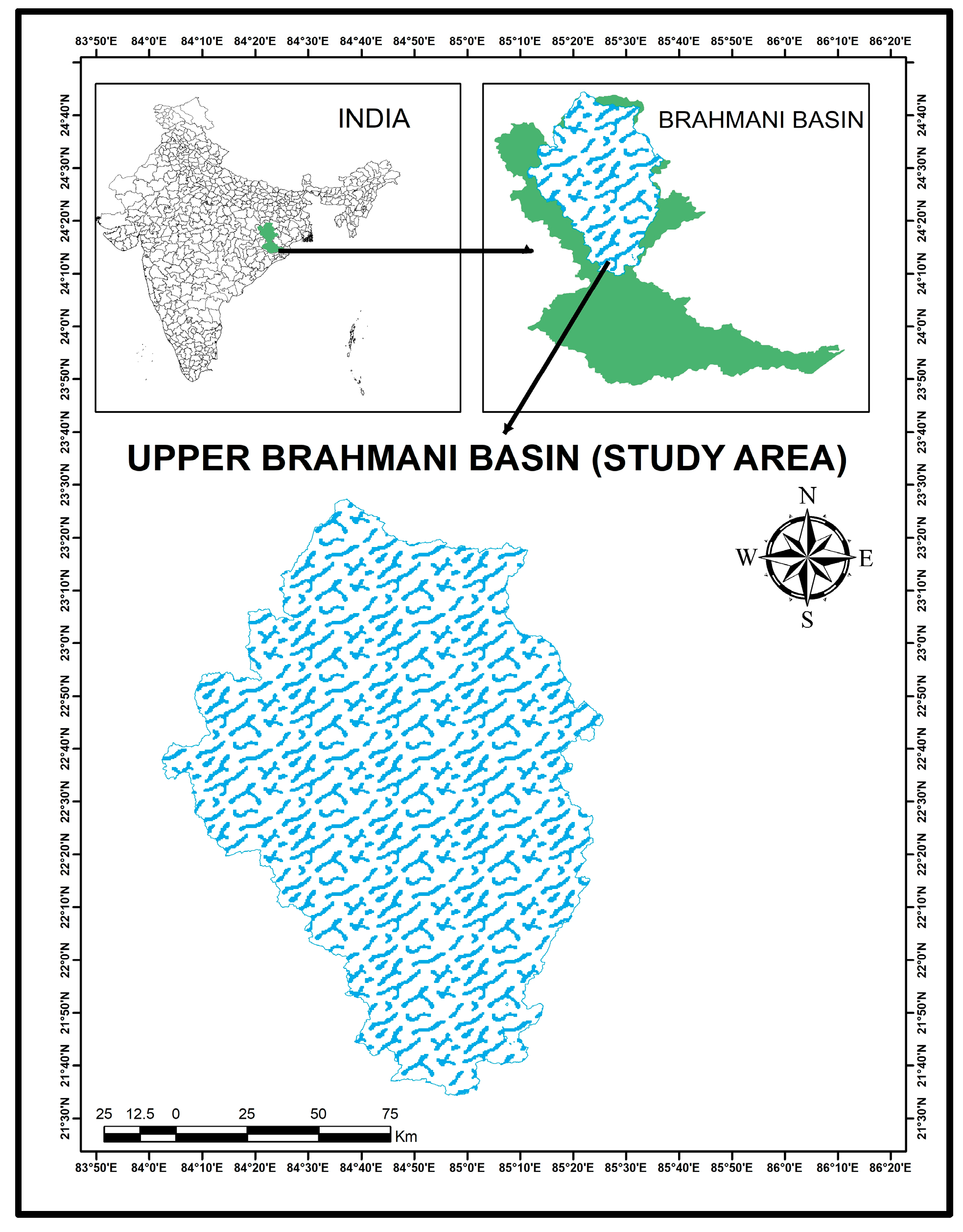
2.1. Description of the Study Area and Data Collection

Brahmani Basin is located in the Indian peninsula’s states of Chhattisgarh, Jharkhand, and Orissa [18], between latitudes of 20°28′ to 23°35′ N and longitudes of 83°52′ to 87°30′ E (Figure 1). It lies between the Mahanadi Basin on the right and the Baitarani Basin on the left. Brahmani is the second-largest river system in the state of Orissa. Two major tributaries, viz. the Sank and Koel, join together at Vedvyas near Rourkela in Odisha and the river system is named Brahmani hereafter. Due to its location close to the Bay of Bengal, Odisha is a natural disaster-prone state. Odisha accounts for 57.34% of the total catchment area of the Brahmani system out of a total of 22,576 square kilometers.
The Rengali dam is located in the middle of the Brahmani River dividing its catchment area into two separate entities. The river Brahmani develops into a massive turbulent waterway during floods, posing a threat to life and properties downstream of the Brahmani River. It is necessary to anticipate the rainfall in the upper catchments to manage the water flow downstream of the river reaches. The study attempts to account for the catchment intercepting up to the Rengali Dam, which intercepts 17,504 square kilometers in the upper half of the river basin.

2.2. Climatic Parameters

Following the availability of raster data for the study region with the same spatial resolution and time, the climatic parameters employed in the simulation studies to forecast predicted rainfall were: temperature, wind speed, solar radiation, and relative humidity. Table 1 contains information on data relating to the time, units, sources, and spatial resolutions that were used in the present study. Data for the present work was collected from Indian Monsoon Data Assimilation and Analysis (IMDAA) which is a national atmospheric reanalysis of data spanning the Indian subcontinent [19]. The IMDAA is the outcome of a partnership between the United Kingdom’s Met Office (MO), India’s National Centre for Medium-Range Weather Forecasting (NCMRWF), and the India Meteorological Department (IMD).

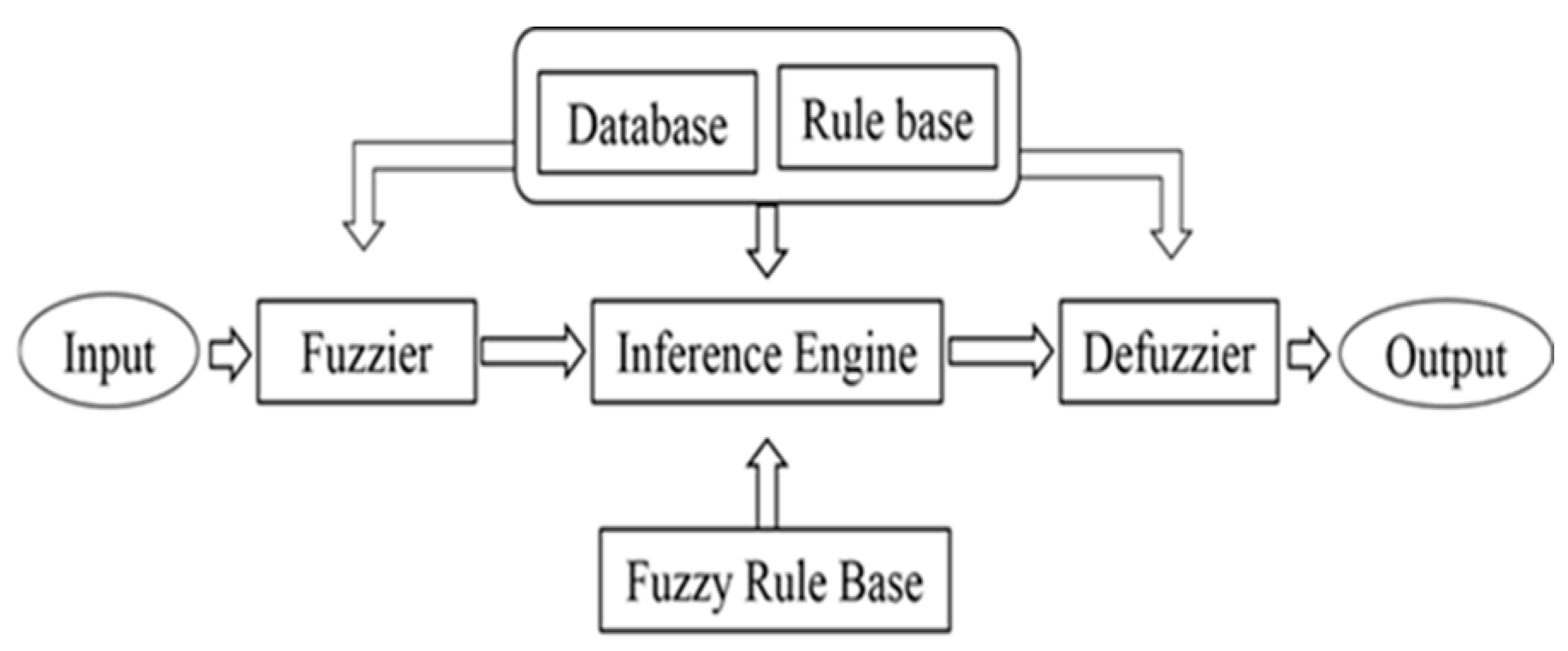
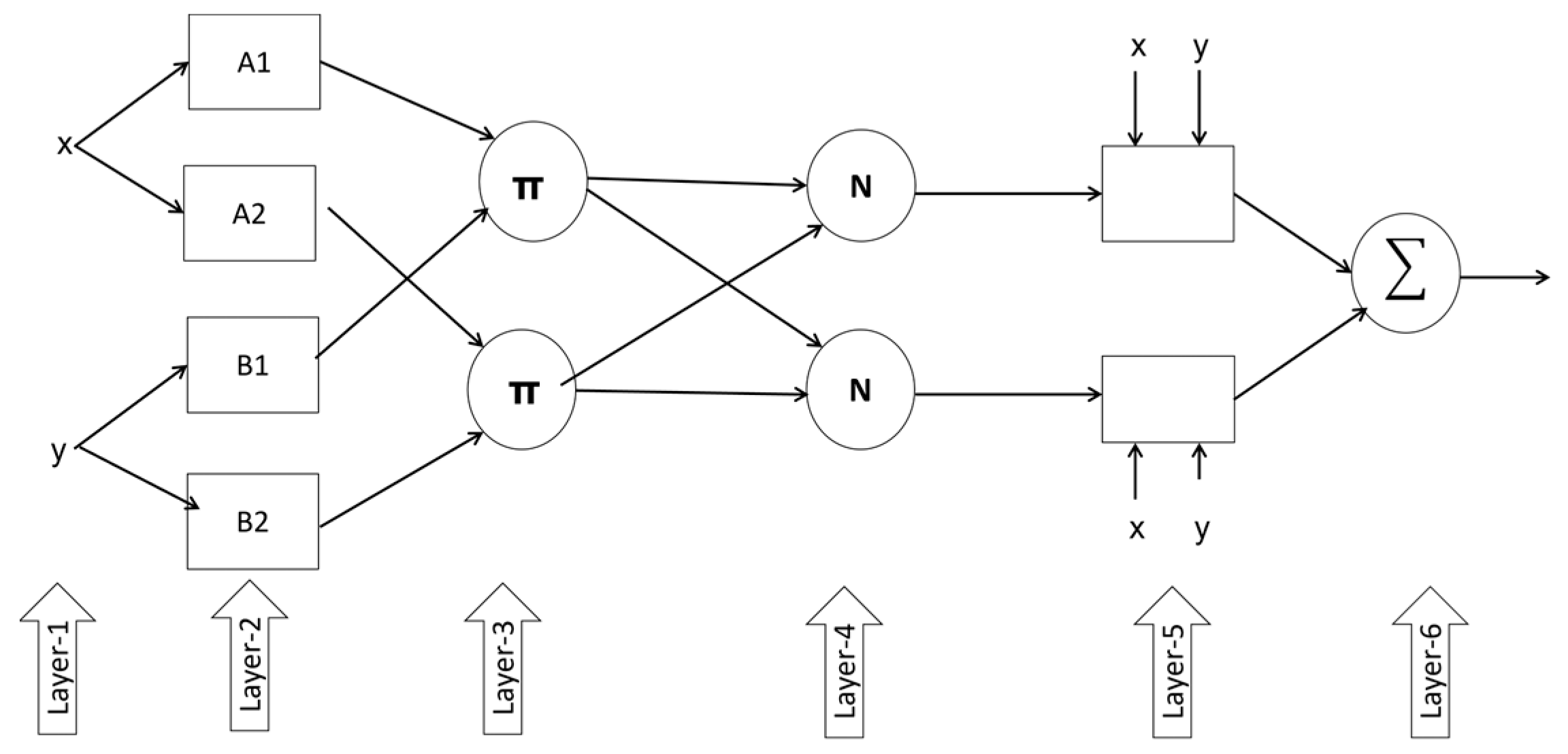
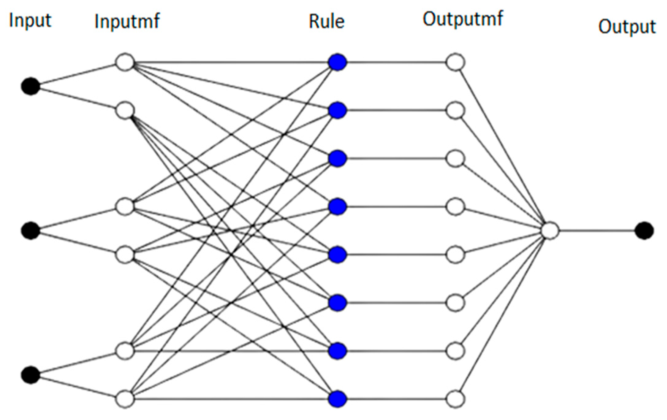
2.3. ANFIS Architecture

For system identification, fuzzy logic and artificial networks are complementary rather than antagonistic, making their joint use desirable. In 1993 Jang [20,21] developed the ANFIS model by combining these two soft-computing tools and building a Sugeno-type fuzzy inference system to transcend the individual limits of ANN and fuzzy logic (FIS). Therefore, ANFIS combines the recognition and adaption capabilities of an ANN with the decision-making capabilities of a fuzzy logic system. As a result, ANFIS overcomes the shortcomings of the ANN and FIS techniques and provides a reliable system identification method, particularly when the input–output link is complicated. In ANFIS, a fuzzy model is created first using rules derived from the system’s input and output data. Then the neural network is used to fine-tune the fuzzy model’s rules to create the best ANFIS model.
ANFIS uses both artificial fuzzy logic and a neural inference system. It has a hybrid approach to estimate the variables, a least square to evaluate the linear variable, and an inaccuracy back-propagation algorithm to estimate dynamical parameters [22]. ANFIS is comprised of five layers. The linear parameter is estimated in the first layer [4]. The idea of fuzzy sets, in which there is no sharp or obvious border, underpins fuzzy logic, which is multi-valued and deals with degrees of membership and truth, unlike two-valued Boolean logic. In fuzzy logic, a membership value is any logical value from the set of real numbers between 0 (totally false) and 1 (entirely true). The function that encodes such values is called a membership function. Artificial neural networks’ learning ability and relational structure are integrated with fuzzy logic’s decision-making process. As for artificial neural networks, ANFIS achieves learning with samples using a training data set. As a result, the most optimal ANFIS structure for solving the associated problem is obtained. The acquired structure is put to the test to see how it reacts to materials [23]. Membership functions are available in a multitude of shapes, including triangular, trapezoidal, Gaussian, sigmoidal, and so on, and are chosen depending on the application. Fuzzy logic contains its own set of logical operators, such as AND, OR, NOT, and others [12]. Each of these operations has its meaning based on the membership value idea. The other key fuzzy logic components are fuzzy rules, which connect the fuzzy sets. If the rule is correct and the antecedent is correct, the consequent must also be correct, following the IF-THEN rule. As shown in Figure 2, the four phases of a typical fuzzy inference system (FIS) are as follows: (a) fuzzification of input variables, (b) evaluation of each rule’s output, (c) aggregation of several rules’ outputs, and (d) defuzzification, which converts fuzzy results into crisp output.
The Takagi–Sugeno FIS is one of the most often used FIS types [3,24]. A fuzzy rule in the Takagi–Sugeno FIS is mostly composed of a linear transformation of crisp inputs rather than fuzzy rules. A typical Takagi–Sugeno FIS rule set contains two fuzzies of IF-THEN rules. The following is a representation of a first-order Sugeno fuzzy model [20] that has two inputs (x and y) and one output (f), as well as Takagi and Sugeno’s two fuzzy IF-THEN rules:
R U L E 1 :   i f   x   i s   A 1   a n d   y   i s   B 1   t h e n   f 1 = p 1 x + q 1 y + r 1
R U L E 2 :   i f   x   i s   A 2   a n d   y   i s   B 2   t h e n   f 2 = p 2 x + q 3 y + r 2
where the premise parameters are pi, qi, and ri. The user defines the premise parameters, which must be optimized using the ANFIS training method. In a fuzzy system with two membership functions, A1 and A2 represent the input x membership functions, while B1 and B2 represent the input y membership functions. Figure 3 shows the ANFIS architecture with two input parameters (x, y) and one output parameter (f). It is worth noting that each layer’s node has the same functions described in the sections below. The output of the layer node ith is represented by Ol,i. The layers are described below.
LAYER 1: Each node i in this layer is an adaptive node with the following node function:
O 1 ,   i = μ A i x   f o r   i = 1 ,   2
O 1 ,   i = μ B i 2 y   f o r   i = 1 ,   2
where µ, x, or y are the nodes representing input variables for i and Ai or Bi−2 are linguistic labels (small or large). In other words, Ol,i specifies the extent to which the provided input x or y meets the quantifier and it is the membership grade of a fuzzy set A and B (A1, A2, B1, or B2) as A′s and B′s membership functions, respectively. Any appropriate parameterized membership function can be used including triangular, trapezoidal, Gaussian, bell, and other forms. In this study, a generalized bell-shaped membership function was used.
LAYER 2: Each node in this layer is a circular junction, and the layer’s output is generated using the following Equation (5) as the product of all incoming signals provided as:
O 2 ,   i = W = μ A i x μ B i y , i = 1 , 2
The rule’s firing strength is represented by each node output, indicating that this layer determines the rule’s strength.
LAYER 3: Each node decides a fixed cluster, which calculates the following ratio of each ith rule’s firing strength to the total of all rule firing strengths provided as:
O 3 ,   i = W i ¯ f i = W i W 1 + W 2   , i = 1 , 2
LAYER 4: The nodes in this layer are all adaptable, having the function provided as:
O 3 ,   i = W i ¯ f i = W i ¯ p i x + q i y + r i       f o r   i = 1 ,   2
The succeeding parameters of this layer are pi, qi, and ri, whereas W i ¯ is the normalized firing strength generated from layer 3. These parameters show optimum values after the ANFIS learning algorithm.
LAYER 5: This is the final layer, which contains only one circular node that accumulates all the incoming signals from layer 4 to determine the overall output provided as:
O v e r a l l   o u t p u t = O 5 , 1 = f = ω i ¯ f i = i ω i f i i ω i
Only the adaptive nodes may be altered based on the user’s requirements. All circular nodes are fixed, whereas square nodes are flexible. This ANFIS method, which employs the Takagi–Sugeno–Kang (TSK) first-order model, is used to estimate the rainfall. A hybrid learning algorithm is chosen as a rainfall forecast among the numerous types of supervised learning algorithms. The fact that a multi-task learning algorithm has been widely utilized can be a good reason to employ it [25,26,27,28]. One of the benefits of ANFIS is that it mixes ANN and fuzzy systems, generating fuzzy IF-THEN rules with proper membership functions that may learn anything from the imprecise data input and lead to an inference utilizing ANN learning skills. Another advantage is that it can make excellent use of the self-learning capabilities of neural networks and memory capacities, resulting in a more stable training process. The Root Mean Squared Error (RMSE) is used for testing. If RSME is small enough, ANFIS is considered to have effectively finished the training process.

Development of an ANFIS Univariate Time Series Forecasting Model

Three-time series inputs R(t), R(t − 1), and R(t − 2) and one output R(t + 1) compensate for the ANFIS architecture used in this study. The inputs are monthly average rainfall data, which the ANFIS model uses to forecast monthly rainfall. The ANFIS framework is designed as a three-layered model with input, output, and hidden layers. The hidden layer is employed for the rainfall prediction technique with Gaussian membership functions. The ANFIS-GRID fuzzy inference system is a hybrid system in which the data space is divided by grid partition into rectangular subspaces by the use of axis-paralleled partition on the basis of the prespecified number of membership functions (MFs) and their types in the dimensions. The prediction model’s input–output structure may be expressed using the following equations:
I n p u t : W t = R t , R t 1 , R t 2
O u t p u t : s t = R t + 1
where R(t + 1) denotes the forecasted data and R(t), R(t − 1), and R(t − 2) denote previous periods. The data (both input and output) for training and testing were normalized in the range [−1, 1] using the following equation:
R n o r m = 2 · R R m i n R m a x R m i n 1
where Rnorm = normalized value of data, Rmax = maximum value of data, and Rmin = minimum value of data. The ANFIS model considered in this study used the Gaussian membership function (MF) with MF type “Constant”. It is to be noted that the grid partition technique is used here to figure out the number of MFs. Incidentally, this technique partitions the domains of the input variables into a number of fuzzy sets. A rule is formed by a combination of these fuzzy sets. The rule set covers the entire input space by using all possible combinations of the input fuzzy sets. The grid partition technique is then applied to generate membership functions for the parameters and to generate the optimized rules of a given data set. The ANFIS structure is shown in Figure 4. White circles represent the membership functions while the black ones represent input and output.

3. Results and Discussion

Here the performance of the developed model along with the parametric analysis are discussed.

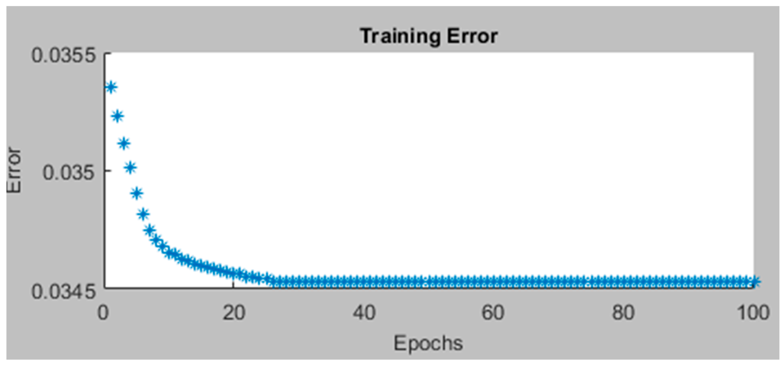
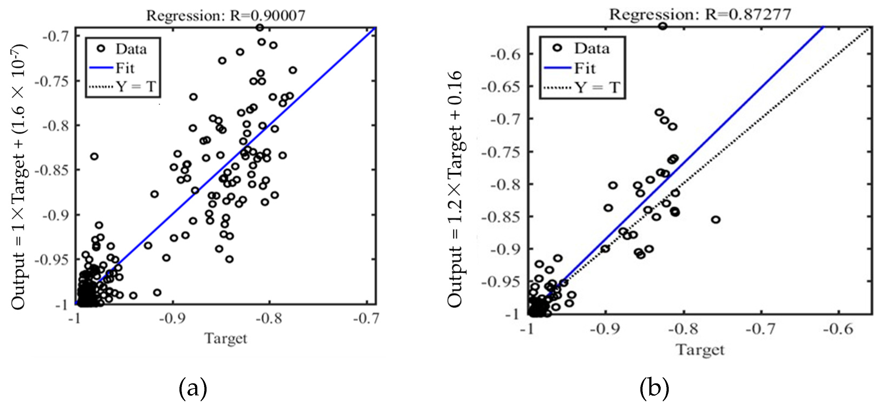
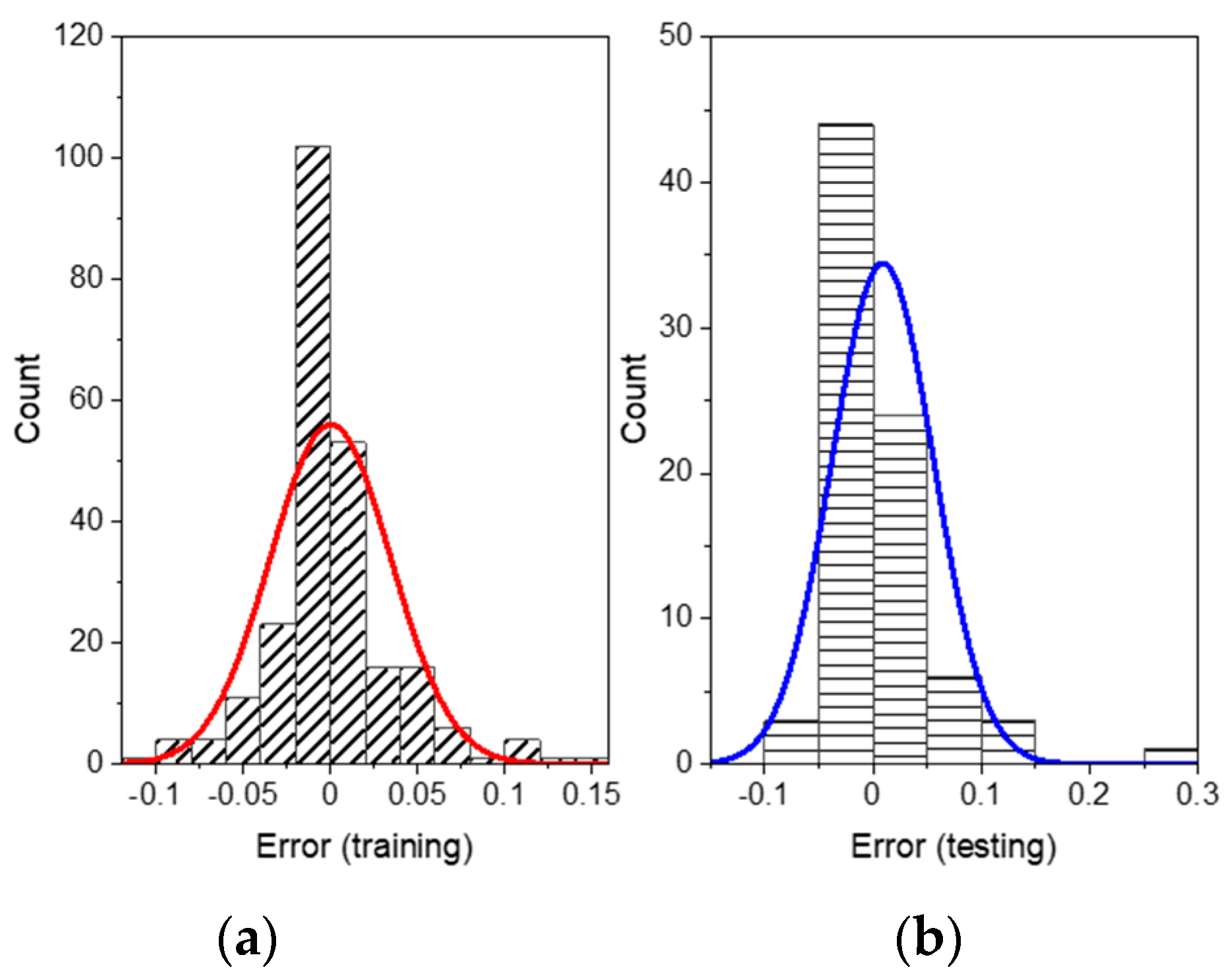
3.1. Setup of the Proposed ANFIS Model and Evaluation of Its Performance

Once the grid partition technique was applied, 23 membership functions were identified. Altogether, 100 epochs were found to be sufficient for obtaining a constant error value (Figure 5).
The performance of the input parameters was assessed by developing and training ANFIS models based on each input parameter. The input parameters having the greatest influence on the output were used effectively to anticipate the output. Statistical indicators such as the root mean square error (RMSE) and the coefficient of determination R2 were used to safeguard this evaluation. Table 2 and Table 3 include the details for the membership functions and constants, respectively.
Figure 6a,b show the training and testing data regression plots, respectively. Seventy-five percent (22.5 years from 1983 to 2006) of the data was set aside for training and twenty-five percent for testing (7.5 years from 2006 to 2020). The system’s output was checked to see if it met the given target. If this was not the case, a new network design or learning approach was introduced to improve the learning method. The R-values of 0.90 during training and 0.87 during testing indicated that the forecasting model had outstanding generalization performance due to its ability to predict the testing data reasonably.
The error distribution is shown in Figure 7. It was found that the peak of the normal distribution curve was very close to zero in both training and testing data sets.
The developed model was used to forecast rainfalls over the period from 2011 to 2020 and the outcomes were compared with the actual data as shown in Figure 8. The computed data appear to be in good agreement with the actual ones.
In particular, the Mean Square Error (MSE) and the Mean Absolute Percentage Error (MAPE) were computed to evaluate the performance of the developed forecasting model. The values of MSE and MAPE for each year under investigation, from 2011 to 2020, are provided in Table 4. The results reveal that the forecasting approach using ANFIS match the observed values satisfactorily.

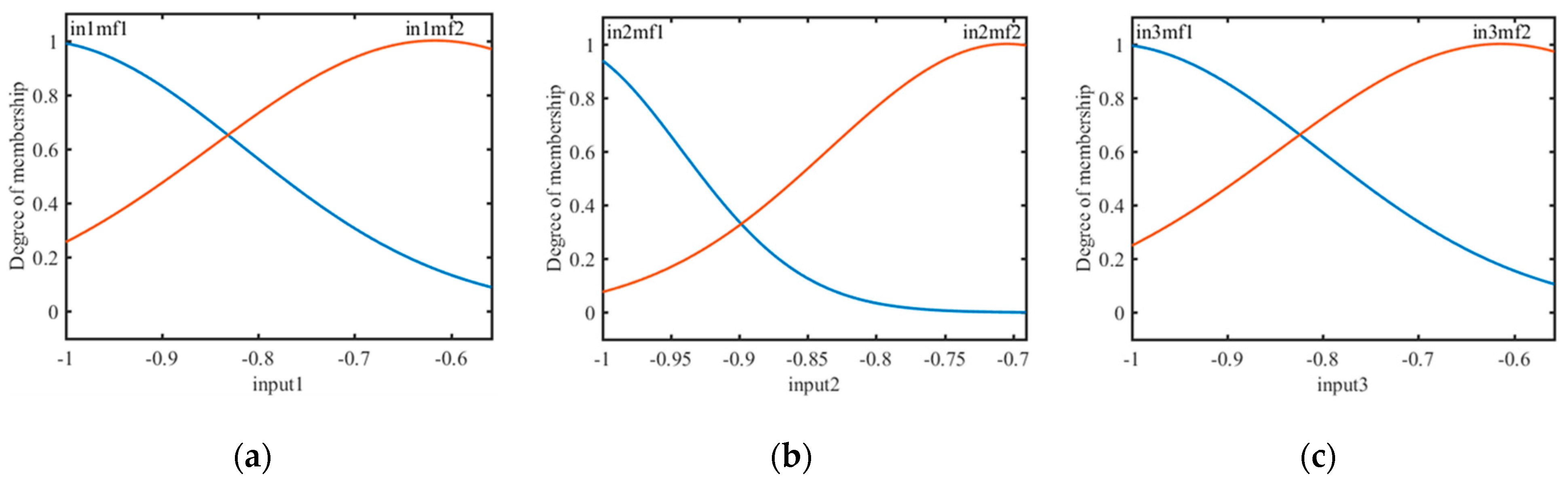
3.2. Parametric Analysis

A degree of membership function in the y-axis represents the degree to which a given input belongs to a particular set or category, typically represented as a value between 0 and 1. In fuzzy logic and fuzzy set theory, a degree of membership function is used to define the membership of an element in a set. It is often represented as a curve or a graph, with the x-axis representing the input and the y-axis representing the degree of membership. The variations in the MFs for each input parameter are shown in Figure 9a–c. A surface plot in fuzzy logic is a three-dimensional representation of a fuzzy set or a membership function. It is used to visualize the degree of membership of an input point in a fuzzy set, with the x- and y-axes representing the input variables and the z-axis the degree of membership.
Here The surface plot shows the shape and boundaries of the fuzzy set, as well as the interactions between the input variables. This is a useful tool for analyzing and understanding complex fuzzy systems, and helped in the design and optimization of fuzzy controllers and other fuzzy logic-based applications. The surface plots are shown in Figure 10a–c. They explain the combined effect of the influencing parameters. While drawing the surface plot, two parameters varied within their highest and lowest ranges while for the remaining parameter it was considered the value of its median.

3.3. Development of an Empirical Expression

The objective of the present study was a step-by-step procedure for developing an empirical equation to forecast the rainfall in the study area. The following procedure was developed in the Matlab platform:
Step1: Normalization of the inputs
For a set of inputs, i.e., [I1, I2, I3], within the considered range, the normalization was performed using Equation (11). The normalized input set became [I1n, I2n, I3n].
Step2: Calculation of firing strength for the ANFIS rules
In the present model, eight rules were provided, which are represented by W1 to W8:
W1 = [I1 MF1] × [I2 MF1] × [I3 MF1]
W2 = [I1 MF1] × [I2 MF1] × [I3 MF2]
W3 = [I1 MF1] × [I2 MF2] × [I3 MF2]
W4 = [I1 MF1] × [I2 MF2] × [I3 MF2]
W5 = [I1 MF2] × [I2 MF1] × [I3 MF1]
W6 = [I1 MF2] × [I2 MF1] × [I3 MF2]
W7 = [I1 MF2] × [I2 MF2] × [I3 MF1]
W8 = [I1 MF1] × [I2 MF2] × [I3 MF2]
where Ii MFj corresponds to ith input and jth MF. The Gaussian membership function was represented by the following equation (Equation (13)):
I i M F i = e ( x c ) 2 2 σ 2
Step 3: Calculation of normalized output
The normalized output On was calculated from the relationship provided as
O n = W 1 × Z 1 + W 2 × Z 2 + . . + W 8 × Z 8 W 1 + W 2 + . . + W 8
where −1 ≤ On ≤ 1.
Step 4: De-normalization of On
The de-normalization of On was carried out using the following equation (Equation (15)):
O = 0.5 × O n + 1 × O max O min + O min
For the Upper Brahmani Basin, the future rainfall was projected using the above step-by-step strategy. The assumption in the present study was that the observed prediction follows nearly the same trend over the upcoming years and that the change in land use and the land cover does not vary much.

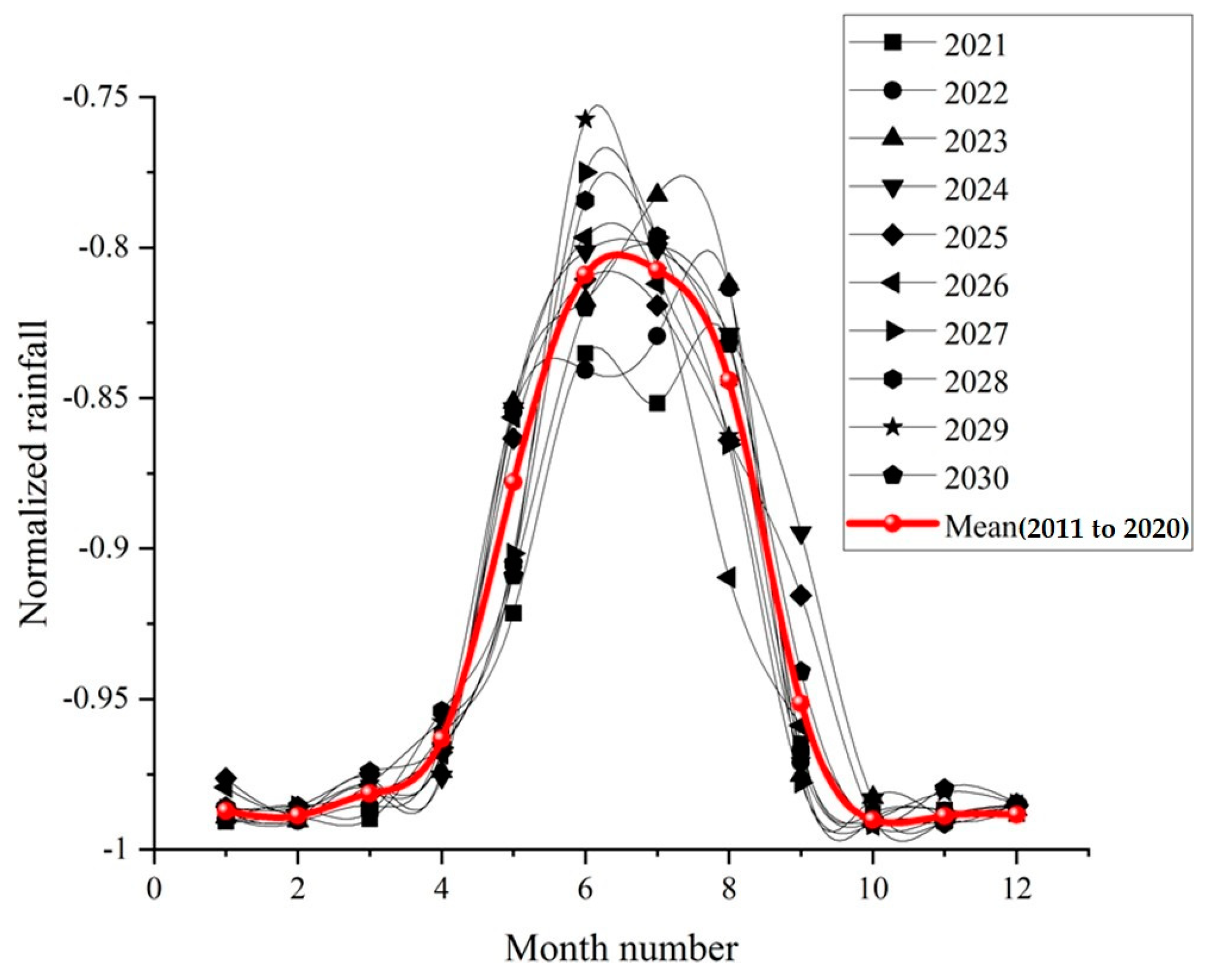
3.4. Forecasting Rainfalls for the Period 2021–2030 by Using the Developed Empirical Equation

As shown in Figure 8, the constructed empirical equation (Equation (15)) predicts monthly rainfall, which yields acceptable results. The predicted monthly rainfalls from 2021 to 2030 are shown in Figure 11. The proposed modeled equation offered excellent results for the upper Brahmani River basin, as seen in Figure 11. The variations from June to September were attributed to an irregular monsoon climate. However, these variations are within acceptable limits. Moreover, the highest rainfall was forecasted for the period June–August, which is a striking characteristic of the monsoon climate. Hence the present model appears to forecast rainfall with reasonable accuracy.
The physical mechanisms behind changes in rainfall forecast between 2021 and 2030 using Adaptive Neuro-Fuzzy Inference System (ANFIS) is not specific and can be different based on the region and the time frame of the forecast. However, some possible factors that can affect the forecast include changes in the ocean–atmosphere circulation patterns, such as El Niño Southern Oscillation (ENSO) and the Indian Ocean Dipole (IOD), which can influence the distribution of precipitation over different regions. Climate change can also affect the precipitation forecast by altering the atmospheric circulation patterns, leading to changes in the intensity and frequency of extreme weather events such as droughts and floods. Additionally, changes in land use and land cover, such as deforestation, urbanization, and land-use change, can affect the local water cycle by altering the amount of water available for evaporation and the energy balance at the surface, which in turn can affect the precipitation forecast.
It is important to note that ANFIS is an artificial intelligence-based model, which uses historical data and the relationships between input and output parameters to make predictions, but it may not always be able to capture the underlying physical processes that drive the forecast. Therefore, it is always important to consider the limitations of the model and the assumptions made when interpreting the results.

4. Conclusions

In the present study, a regional analysis was performed to develop a rainfall forecasting model for the Upper Brahmani Basin in India. The study area lies in the sub-tropical region, but it is relatively close to the equatorial warm climate region. Weather data from the past four decades were considered to develop a model that is based on fuzzy algorithms. Using the trained fuzzy model based on the univariate forecasting model and the sensitivity analysis, the following major inferences were drawn.
The Gaussian membership function with the hybrid algorithm can predict monthly average rainfalls with satisfactory accuracy with R-values of 0.90 and 0.87 at training and testing stages, respectively. The comparison of the model predictions with the observations (Figure 8) for the years from 2011 to 2020 indicate the adequacy of the forecasting model for future rainfalls. Therefore, a new empirical expression (Equation (15)) using the immediate three preceding inputs was applied to forecast future rainfalls. The sensitivity analysis indicates that rainfalls of the previous two months is an important parameter to forecast the average monthly rainfall. This trend is in good agreement with the climatic conditions of sub-tropical regions where seasonal variation is less significant.
The results can be useful in the future planning, design, and operation of water resource projects. They may also be used for micro-level watershed planning and, especially, water budgeting. The lack of knowledge on future rainfalls is a significant problem that needs to be addressed in the development of micro-level watersheds, which are from 800 to 1000 hectares in size. The proposed forecasting model might be of consistent use for regions lying in similar latitudes, but its testing in similar basins in other locations is auspicious.

Author Contributions

Conceptualization, M.M.R. and K.C.P.; methodology, M.M.R. and K.C.P.; software, S.K.S.; validation, M.M.R., K.C.P. and A.S.; formal analysis, M.M.R. and K.C.P.; investigation, M.M.R. and K.C.P.; resources, K.C.P.; data curation, M.M.R.; writing—M.M.R.; original draft preparation, M.M.R. and S.K.S.; writing—review and editing, A.S. and G.O.; visualization, K.C.P.; supervision, K.C.P. All authors have read and agreed to the published version of the manuscript.

Funding

This research received no external funding.

Data Availability Statement

The data can be obtained from the corresponding author on request.

Conflicts of Interest

The authors declare no conflict of interest.

References

  1. Rasel, H.M.; Imteaz, M.A. Application of Artificial Neural Network for seasonal rainfall forecasting: A case study for South Australia. In Proceedings of the World Congress on Engineering, London, UK, 29 June–1 July 2016. [Google Scholar]
  2. del Real, A.J.; Dorado, F.; Durán, J. Energy demand forecasting using deep learning: Applications for the French grid. Energies 2020, 13, 2242. [Google Scholar] [CrossRef]
  3. Nourani, V.; Komasi, M. A geomorphology-based ANFIS model for multi-station modeling of rainfall-runoff process. J. Hydrol. 2013, 490, 41–55. [Google Scholar] [CrossRef]
  4. Calp, M.H. A hybrid ANFIS-GA approach for estimation of regional rainfall amount. GU J. Sci. 2019, 32, 145–162. [Google Scholar]
  5. Emamgholizadeh, S.; Moslemi, K.; Karami, G. Prediction the groundwater level of Bastam Plain (Iran) by Artificial Neural Network (ANN) and Adaptive Neuro-Fuzzy Inference System (ANFIS). Water Resour. Manage. 2014, 28, 5433–5446. [Google Scholar] [CrossRef]
  6. Bacanli, U.G.; Firat, M.; Dikbas, F. Adaptive Neuro-Fuzzy Inference System for drought forecasting. Stoch. Environ. Res. Risk Assess. 2009, 23, 1143–1154. [Google Scholar] [CrossRef]
  7. Aldrian, E.; Djamil, Y.S. Application of multivariate ANFIS for daily rainfall prediction: Influences of training data size. Makara Sains 2008, 12, 7–14. [Google Scholar] [CrossRef]
  8. Tektas, M. Weather forecasting using ANFIS and ARIMA models. Environ. Res. Eng. Manag. 2010, 51, 5–10. [Google Scholar]
  9. Zhang, X.-d.; Li, A.; Pan, R. Stock trend prediction based on a new status box method and AdaBoost probabilistic Support Vector Machine. Appl. Soft. Comput. 2016, 49, 385–398. [Google Scholar] [CrossRef]
  10. Zhang, X.; Mohanty, S.N.; Parida, A.K.; Pani, S.K.; Dong, B.; Cheng, X. Annual and non-monsoon rainfall prediction modelling using SVR-MLP: An empirical study from Odisha. IEEE Access 2020, 8, 30223–30233. [Google Scholar] [CrossRef]
  11. Kiani, R.S.; Ali, S.; Ashfaq, M.; Khan, F.; Muhammad, S.; Reboita, M.S.; Farooqi, A. Hydrological projections over the Upper Indus Basin at 1.5 °C and 2.0 °C temperature increase. Sci. Total Environ. 2021, 788, 147759. [Google Scholar] [CrossRef]
  12. Mekanik, F.; Imteaz, M.A.; Talei, A. Seasonal rainfall forecasting by adaptive network-based fuzzy inference system (ANFIS) using large scale climate signals. Clim. Dyn. 2016, 46, 3097–3111. [Google Scholar] [CrossRef]
  13. Aftab, S.; Ahmad, M.; Hameed, N.; Bashir, M.S.; Ali, I.; Nawaz, Z. Rainfall prediction in Lahore City using data mining techniques. Int. J. Adv. Comput. Sci. Appl. 2018, 9, 254–260. [Google Scholar] [CrossRef]
  14. Kyada, P.M.; Kumar, P.; Sojitra, M.A. Rainfall forecasting using Artificial Neural Network (ANN) and Adaptive Neuro-Fuzzy Inference System (ANFIS) models. Int. J. Agric. Sci. 2018, 10, 6153–6159. [Google Scholar]
  15. Usha, S.; Priya, S.B. An effective approach for promoting agriculture by predicting rainfall in India by using Machine Learning Techniques. J. Chem. Pharm. Sci.-Special Issue 2016, 37–43. [Google Scholar]
  16. Khajure, S.; Mohod, S.W. Future weather forecasting using soft computing techniques. Procedia Comput. Sci. 2016, 78, 402–407. [Google Scholar] [CrossRef] [Green Version]
  17. Chantry, M.; Christensen, H.; Dueben, P.; Palmer, T. Opportunities and challenges for machine learning in weather and climate modelling: Hard, medium and soft AI. Philos. Trans. A Math. Phys. Eng. Sci. 2021, 379, 20200083. [Google Scholar] [CrossRef]
  18. Novitasari, D.C.R.; Rohayani, H.; Suwanto; Arnita; Rico; Junaidi, R.; Setyowati, R.D.; Pramulya, R.; Setiawan, F. Weather parameters forecasting as variables for rainfall prediction using Adaptive Neuro Fuzzy Inference System (ANFIS) and Support Vector Regression (SVR). J. Phys. Conf. Ser. 2020, 1501, 012012. [Google Scholar] [CrossRef]
  19. Rani, S.I.; Arulalan, T.; George, J.P.; Rajagopal, E.N.; Renshaw, R.; Maycock, A.; Barker, D.M.; Rajeevan, M. IMDAA: High-resolution satellite-era reanalysis for the Indian monsoon region. J. Climate 2021, 34, 5109–5133. [Google Scholar] [CrossRef]
  20. Jang, J.-S.R.J. ANFIS: Adaptive-Network-Based Fuzzy Inference System. IEEE T. Syst. Man Cyb. 1993, 23, 665–685. [Google Scholar] [CrossRef]
  21. Karaboga, D.; Kaya, E. Adaptive network-based fuzzy inference system (ANFIS) training approaches: A comprehensive survey. Artif. Intell. Rev. 2019, 52, 2263–2293. [Google Scholar] [CrossRef]
  22. Kişi, Ö. Daily pan evaporation modelling using a neuro-fuzzy computing technique. J. Hydrol. 2006, 329, 636–646. [Google Scholar] [CrossRef]
  23. Rao, K.K.; Kulkarni, A.; Patwardhan, S.; Kumar, B.V.; Kumar, T.V.L. Future changes in precipitation extremes during northeast monsoon over south peninsular India. Theor. Appl. Climatol. 2020, 142, 205–217. [Google Scholar] [CrossRef]
  24. Ashrafi, M.; Chua, L.H.C.; Quek, C.; Qin, X. A fully-online Neuro-Fuzzy model for flow forecasting in basins with limited data. J. Hydrol. 2017, 545, 424–435. [Google Scholar] [CrossRef]
  25. Suparta, W.; Samah, A.A. Rainfall prediction by using ANFIS times series technique in South Tangerang, Indonesia. Geod. Geodyn. 2020, 11, 411–417. [Google Scholar] [CrossRef]
  26. Mosavi, A.; Ozturk, P.; Chau, K.-W. Flood prediction using Machine Learning models: Literature review. Water 2018, 10, 1536. [Google Scholar] [CrossRef] [Green Version]
  27. Sharma, A.; Goyal, M.K. A comparison of three soft computing techniques, Bayesian Regression, Support Vector Regression, and Wavelet Regression, for monthly rainfall forecast. J. Intell. Syst. 2017, 26, 641–655. [Google Scholar] [CrossRef]
  28. Tarun, G.B.S.; Sriram, J.V.; Sairam, K.; Sreenivas, K.T.; Santhi, M.V.B.T. Rainfall prediction using Machine Learning Techniques. Int. J. Innov. Technol. Explor. Eng. 2019, 8, 957–963. [Google Scholar]
Figure 1. Map of the study area with localization of the Upper Brahmani Basin within the India map.
Water 15 00499 g001
Figure 2. Scheme for the Fuzzy Interface System (FIS).
Water 15 00499 g002
Figure 3. Scheme for the ANFIS architecture.
Water 15 00499 g003
Figure 4. Structure of the ANFIS model considered in this study.
Water 15 00499 g004
Figure 5. Error as a function of epochs for the ANFIS model considered in this study.
Water 15 00499 g005
Figure 6. Comparison of the ANFIS outcomes with the actual data for the (a) training and (b) testing data set.
Water 15 00499 g006
Figure 7. Error distribution for the (a) training and (b) testing data sets.
Water 15 00499 g007
Figure 8. Comparison of forecasted results with actual ones for the period 2011 to 2020. The x-axis refers to the months from January (i.e., 1) to December (i.e., 12), the y-axis refers to the normalized rainfall, and the given year is provided at the top of each graph.
Water 15 00499 g008
Figure 9. Membership functions for (a) R(t), (b) R(t − 1), and (c) R(t − 2).
Water 15 00499 g009
Figure 10. Combined effects of (a) R(t) and R(t − 1), (b) R(t) and R(t − 2), and (c) R(t − 1) and R(t − 2) on the output.
Water 15 00499 g010
Figure 11. Forecasted normalized monthly rainfall from 2021 to 2030, along with the average rainfall (from 2011 to 2020).
Water 15 00499 g011
Table 1. Details of the input data set for the ANFIS model to evaluate future rainfall data.
ParametersRainfallTmaxTminRHWSSR
Unitmm/day°C°C%m/skw-hr/m2/day
FrequencyDaily
Time1983–2020
SourceIndian Monsoon Data Assimilation and Analysis (IMDAA)
Spatial Resolution0.25° × 0.25°
Table 2. Parameters of gbell membership functions.
InputsMembership Function
UnitMF1MF2
σCσC
I10.2152−1.0310.2323−0.6165
I20.08962−1.0320.1304−0.7043
I30.2201−1.0240.2318−0.6137
Table 3. List of constant values.
InputConstant
1−1.084
2−0.783
3−1.099
4−0.6866
5−0.8932
6−0.9446
7−0.5058
8−0.9508
Table 4. Performance indices MSE and MAPE to evaluate the prediction effects of the proposed ANFIS model.
Year2011201220132014201520162017201820192020
MSE0.0070.0020.0020.0010.0030.0010.0050.0020.0010.003
MAPE7.044.153.932.544.493.224.783.802.725.09
Disclaimer/Publisher’s Note: The statements, opinions and data contained in all publications are solely those of the individual author(s) and contributor(s) and not of MDPI and/or the editor(s). MDPI and/or the editor(s) disclaim responsibility for any injury to people or property resulting from any ideas, methods, instructions or products referred to in the content.

