
Inflow Scenario Generation for the Ethiopian Hydropower System


1
School of Electrical and Computer Engineering, Addis Ababa Institute of Technology, Addis Ababa 385, Ethiopia
2
School of Electrical Engineering and Computer Science, KTH Royal Institute of Technology, SE-10044 Stockholm, Sweden
*
Author to whom correspondence should be addressed.
†
Current address: Division of Electric Power and Energy Systems, KTH Royal Institute of Technology, Teknikringen 33, SE-10044 Stockholm, Sweden.
Water 2023, 15(3), 500; https://doi.org/10.3390/w15030500
Submission received: 25 November 2022
/
Revised: 20 January 2023
/
Accepted: 24 January 2023
/
Published: 27 January 2023
(This article belongs to the Section Water-Energy Nexus)
Abstract
:In a hydropower system, inflow is an uncertain stochastic process that depends on the meteorology of the reservoir’s location. To properly utilize the stored water in reservoirs, it is necessary to have a good forecast or a historical inflow record. In the absence of these two pieces of information, which is the case in Ethiopia and most African countries, the derivation of the synthetic historical inflow series with the appropriate time resolution will be a solution. This paper presents a method of developing synthetic historical inflow time series and techniques to identify the stochastic process that mimics the behavior of the time series and generates inflow scenarios. The methodology was applied to the Ethiopian power system. The time series were analyzed using statistical methods, and the stochastic process that mimics the inflow patterns in Ethiopia was identified. The Monte Carlo simulation was used to generate sample realizations of random scenarios from the identified stochastic process. Then, three cases of inflow scenarios were tested in a deterministic simulation model of the Ethiopian hydropower system and compared with the actual operation. The results show that the generated inflow scenarios give a realistic output of generation scheduling and reasonable reservoir content based on the actual operation.
1. Introduction
The generation and operation of hydropower plants are highly dependent on weather conditions in the particular location of the reservoirs. To efficiently utilize hydropower, it is, therefore, necessary to have an inflow forecast. Prior knowledge about the reservoir inflow would help manage the water resource properly throughout the year. Otherwise, in case of a low inflow year, the water in the reservoirs might be used up before the next rainy season, and the reservoirs will be empty. Consequently, there will be a lot of load shedding until the reservoirs fill up again, which can also affect the start content of the reservoirs for the next planning period. On the other hand, in case of an unexpectedly high inflow year, we may end up spilling much water, and reservoirs could also be flooded.
In Ethiopia and many other countries in East Africa, hydropower is the dominant source of electric power. According to the international hydropower association (IHA) 2022 hydropower status report, Africa’s energy generation by hydropower is 146 TWh in 2021, 21% of this generation being from Eastern African countries, of which 45% is from Ethiopia [1]. Most of the inflow is during the rainy season, July to September (Kiremt).
The water in the rainy season is stored in large reservoirs to be distributed over the remaining part of the year until the next rainy season comes again. Therefore, hydropower planners need inflow forecasts for at least one year with a sufficient time resolution. However, the challenge is the limited availability of necessary data. For example, there are no accurate water inflow measurements for each reservoir. Therefore, there is a need to develop a method to randomly generate realistic inflow scenarios from the available data sets, including hydropower generation data and satellite precipitation measurements.
Hydrologists use watershed models to estimate stream flow, surface run-off, water quality, flood management, and water management. The review of different watershed modeling, the use of AI techniques, artificial neural networks (ANNs), fuzzy logic (FL), genetic algorithms (GAs) to improve upon or replace traditional physically-based watershed modeling techniques, and detailed discussions of individual watershed models are presented in [2]. The precipitation-runoff modeling system (PRMS) is one of the watershed modeling software used to simulate precipitation and snow melt-driven movement of water to produce the daily system response and streamflow for a basin [3]. PRMS is applied to simulate rainfall runoff in the Zamask–Yingluoxia subbasin of the Heihe River Basin in [4]. The current and future geographic information systems (GIS) trends and remote sensing technologies in watershed modeling are reviewed in [5]. It is demonstrated in [6] that the surface water assessment tool (SWAT) provides a better streamflow estimate with Next Generation Weather Radar (NEXRAD) precipitation input than rain gauge inputs. The accuracy of the model results suggests that NEXRAD is a good alternative to rain gauge data and can be extremely valuable in large watersheds without readily available rain gauge data. In order to utilize the watershed modeling tools, for example, SWAT, we need to have input about soil, land use and management, elevation, and daily rainfall to predict daily stream flow. In addition, we need expert knowledge of hydrology and the use of watershed models, which is beyond the scope of this research work.
There are other methods proposed in the literature that generate random time series, for example, stochastic processes. In [7], a stochastic process estimation based on the concept of aggregation is presented, and the aggregation of periodic autoregressive (PAR) and periodic autoregressive-moving average (PARMA) models for the seasonal and annual flows of the Niger river are used to illustrate the concept. Inflow is modeled as a stochastic variable by first-order autoregressive model AR(1) in [8] for a stochastic dual dynamic programming (SDDP) to solve optimal medium-term scheduling in the Norwegian hydropower system. In [9], a non-parametric simulation model is applied to generate synthetic monthly flows from the Beaver River, Australia. A maximum likelihood procedure for estimating the PARMA model of a monthly average river flows time series is presented in [10]; the Kalman filtering algorithm is used to estimate the parameters. A non-linear periodic autoregressive model (PAR(p))scenario generation method based on the vine copula model is presented in [11]; the method incorporates a time dependence more than lag-one, unlike the copula-based models. A monthly stream flow simulation method based on the vine copula model is proposed in [12] for a catchment of the Yellow River basin upstream of the Tangnaihai hydrological station in the north of China. The ARFIMA model, an extension of the Box–Jenkins family, where the differentiation can take fractional values to capture the long-memory effect present in the time series, is used in [13] for generating synthetic hydrological scenarios for the Brazilian hydropower system.
However, almost all of the methods described in the literature are based on well-recorded and organized historical data. In the case of the Ethiopian hydropower system, and most African hydropower systems, where there is a significant gap in the availability of organized data, it is necessary to derive a method to generate synthetic historical series.
Therefore, the first contribution of this paper is to derive a method for generating a synthetic historical time series by combining the available data in hand. The second contribution is to generate realistic inflow scenarios by applying existing methods to identify the stochastic process that mimics the synthetic historical time series. The method is applied to the Ethiopian power system. Finally, the paper demonstrates how the generated scenarios can be applied in Ethiopia’s long-term deterministic hydropower planning model.
This paper is organized as follows. Section 2 presents the materials and methods for deriving the historical time series, the time series analysis, and stochastic model estimation. Then, the study results, synthetic historical time series, scenario generation, and evaluation of the generated inflow scenarios using the deterministic model are presented and discussed in Section 3. Finally, Section 4 concludes the work.
2. Materials and Methods
This section presents the materials and methods used to derive the synthetic historical series and generate the inflow scenarios.
2.1. Study Area, Data, and Materials
The methodology is applied to the Ethiopian power system. Ethiopia is located in the horn of Africa with a 90% hydro-dominated power system. The Ethiopian power system has around thirteen larger hydropower plants. Additionally, three wind power plants and one waste-to-energy plant. These are connected to the national grid [14]. Figure 1 shows the GIS map of the Ethiopian hydropower stations.
Most of the reservoirs are in a different river system. Cascaded systems are Gibe I and II, with Gibe I at the upper stream, and Koka, Awash II and III, with Koka at the upper stream. Beles, sometimes called Tana Beles, Tis Abay I, and Tis Abay II are power plants that source Lake Tana. Lake Tana is the largest lake in Ethiopia, the source of the Blue Nile River located in the northwestern highlands of the country with a surface area of 3200 km2 and an elevation of 1787 m. The lake serves as the reservoir of the Beles hydropower plant with seven spillway gates called Charachara Gates. The spilled water at Charachara is used partly for the Tis Abay fall(Tis Esat, tourist attraction) and partly for power generation at Tis Abay I and II. However, there is yet to be available data about the percentage of water that will be used for power production. Therefore, we treat the Tis Abay I and II power plants as run-of-the-river throughout this study. As a result, we have eight reservoirs, and the generation largely depends on the maximum reservoir level attained during the rainy season (July to September).
The hydropower generation data and the general information about the reservoirs understudy are collected from Ethiopian Electric Power (EEP). Table 1 shows the geographical location and general information about the thirteen Ethiopian hydropower plants connected to the national grid. This study excludes reservoirs that were out of operation during the study, small reservoirs with incomplete information, insignificant effects in operation, and reservoirs under construction during the study time 2018–2019, which are our base years for the actual operation data.
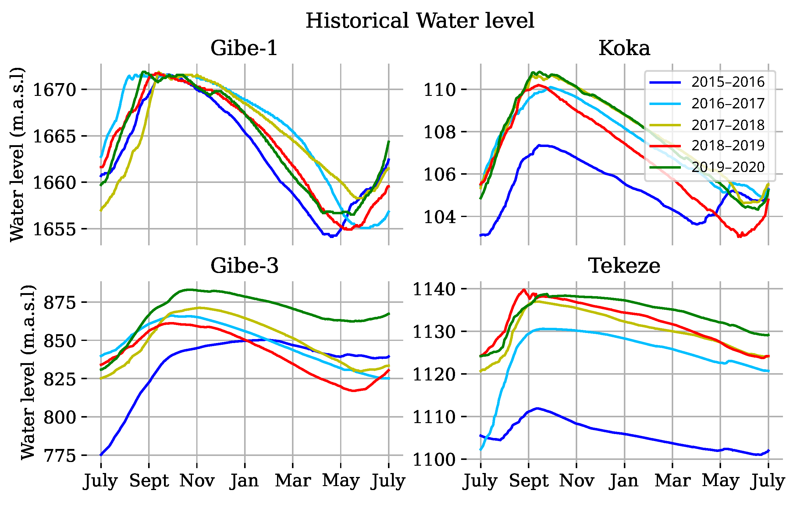
In the actual operation of the Ethiopian power system, the generation planning depends on the historical level of reservoirs and the corresponding energy generated. As an example, Figure 2 shows the five-year history of the reservoir levels for Gibe 1, Gibe 3, Koka, and Tekezé reservoirs.
The water management planning for the dry season starts in October when the reservoir levels start to decrease. The generation schedule considers the three conditions for each generating station.
- Plant’s unique characteristics in relation to the water level (Gibe 1, Gibe 2, and Gibe 3)
- Load forecast and history of generation.
- Downstream facilities (Beles, Fincha, and Koka)
Based on these three conditions, the generation is scheduled following the historical relationship between the reservoir’s water level and power generation. The information in the water level recording can tell us when the reservoir is full and when it starts to drop, which is a precaution to begin water management of the reservoirs. However, it could not tell us the inflows to the reservoir or how much is expected in the future.
The NASA POWER data access viewer (DAV) [15] is used to access the satellite precipitation measurement data based on the latitude and longitude of each reservoir. Ten years of historical precipitation time series from July 2010 to July 2020 are extracted from the DAV for each reservoir in the daily time resolutions. The Matlab Econometric Modeler Application, Version 5.1 (R2018b) [16] is used to perform time series analysis and statistical model identification tests.
2.2. Methods
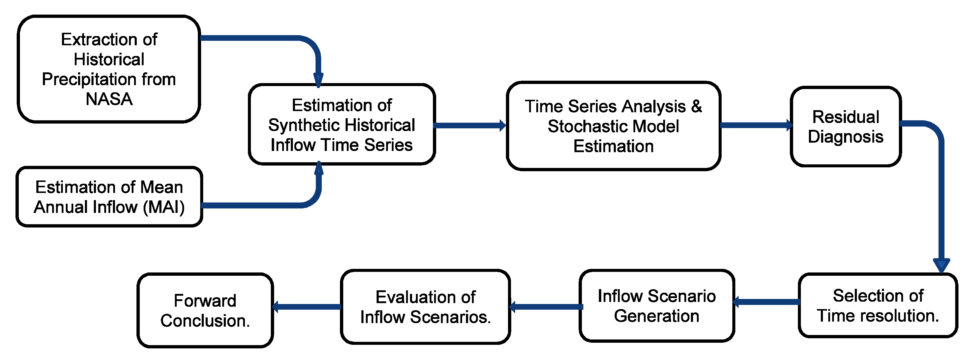
We have developed two steps of processes to generate the inflow scenarios. The first step is to combine the available historical data about hydropower generation and precipitation to estimate synthetic historical inflow time series. As a straightforward solution, we could have used the estimated synthetic historical inflows as scenarios for the future. However, the limited data to estimate the historical series may lead to a series that misses significant variations, and the data might not be sufficient for planning models. Therefore, the second step is to identify a stochastic process that can generate random inflow scenarios, which follow the same pattern as the synthetic historical inflow series. The second step allows us to generate as many scenarios as needed that are not limited by historical data. Figure 3 shows the methodology framework to illustrate the workflow of this paper.
2.2.1. Estimation of Historical Inflow Time Series
In this paper, a method to generate synthetic inflow series from the data available for all the reservoirs is derived. The method used to derive synthetic historical inflow series to the reservoirs is scaling down the mean annual inflow (MAI) of each reservoir based on the percentage precipitation of each reservoir. First, the data for the individual reservoir precipitation measurement is extracted from the NASA DAV based on the geographical location of the power plants in a daily time resolution. Then, the percentage of precipitation over a year is used to distribute the MAI in the same proportion as the precipitation, neglecting delays, topology, and such factors.
where:
Volume inflow of reservoir i in (HE),
Daily precipitation per location of reservoir i in (mm),
Annual precipitation per location of reservoir i.
However, there are no statistics for the MAI of each reservoir. Therefore, we need to estimate the MAI using the available information at hand. The mean annual energy (MAE) generation and the production equivalent are used to approximate the mean annual inflow (MAI) to the reservoirs. The approximation considers electricity generation at the best efficiency and generation approximated as a linear function of discharge. Therefore,
where:
Generation of hydropower plant i in (MW),
Production equivalent of power plant i, (MW/HE).
Discharge from power plant i in (HE).
Mean annual energy generation of power plant i in (MWh).
Mean annual inflow to power plant i in (HE).
HE = Hour equivalent, m3/s of water released during one hour.
Ten years of synthetic historical inflow time series are estimated using Equation (1) for each reservoir in a daily and weekly time resolution.
2.2.2. Time Series Analysis and Stochastic Model Estimation
The most prominent and frequently used method for time series analysis for all applications, such as finance, business, and engineering research, is the Box-Jenkins methodology [17]. We follow this methodology to identify the stochastic process that mimics the inflow time series. The seasonal autoregressive integrated moving average (SARIMA) model from the Econometric modeler Matlab tool is used to estimate the stochastic model.
The time series analysis is performed for the individual reservoir in two sets of inflow time series; one with daily time resolution and the other with weekly time resolution. The objective is to see which resolution best captures the behaviors of the synthetic series and transforms it into the future.
In the selected methodology, the time series are checked for stationarity. Moreover, for a non-stationary series, there is a need for differencing the original series () to reduce the process to a mixed autoregressive-moving average process of the form,
as stated in [17], where:
backward shift operator defined by .
Autoregressive operator.
Constant term.
Moving average operator.
Backward difference operator of order d.
White noise process.
Then the analysis will be performed in the ’differenced’ series ().
Daily Time Resolution
The time series in a daily time resolution is the first set of time series approximated from the available information. The analysis indicates that the reservoirs’ inflow time series in the daily time resolution are non-stationary processes. The analysis of the differenced time series shows that the stochastic processes are seasonal autoregressive integrated moving average processes of various orders.
For example, the differenced time series for Gibe 3 shows that the stochastic process is an autoregressive integrated moving average process (ARIMA) (0,1,3) seasonally integrated with MA(730)(SARIMA(0,1,3)(0,1,2)[365]) with Equation (5).
and for the rest of the reservoirs the process is SARIMA(0,1,2)(0,1,2)[365] with Equation (6)
where:
Seasonal moving average operator.
Weekly Time Resolution
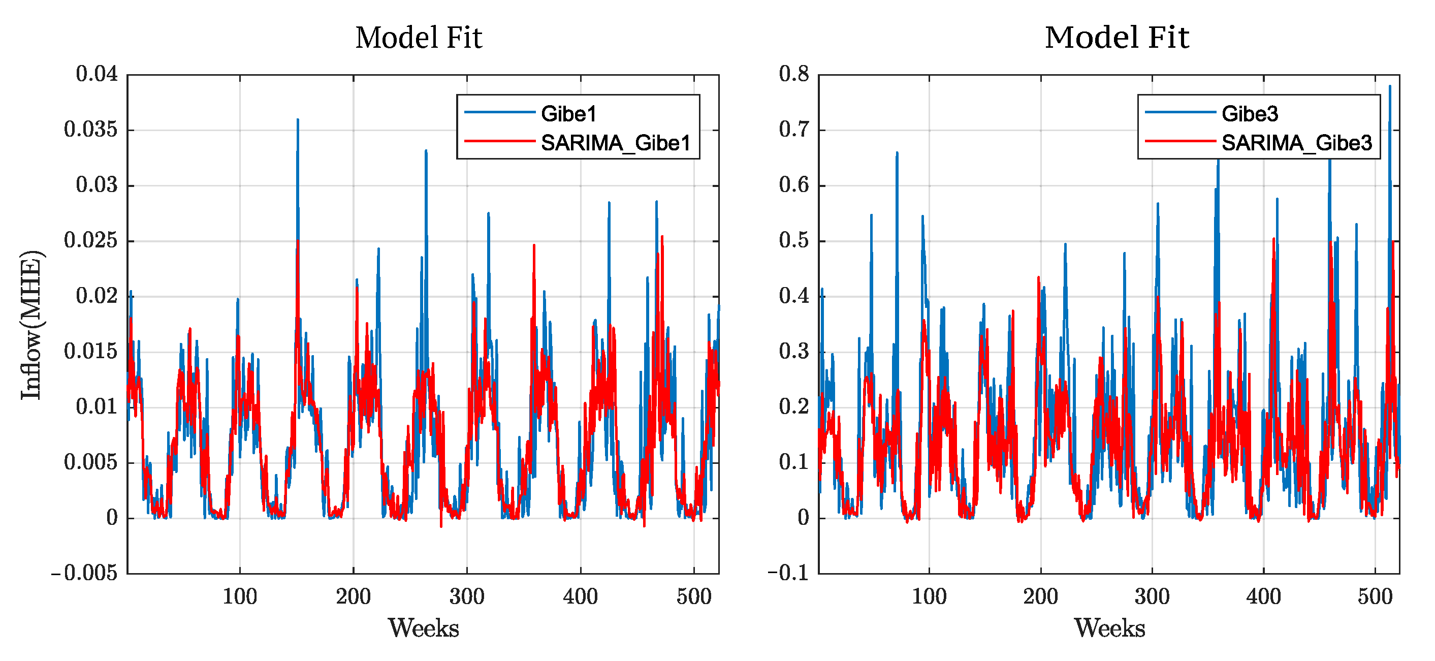
The second set of time series analyzed is the same series reduced to weekly time resolution. The analysis shows that the time series for all the reservoirs are stationary autoregressive models of various orders, AR(1), AR(2), and AR(3) process with the consideration of seasonality equal to the number of weeks in a year (52). For example, the model for Gibe 3 is estimated as SARIMA(2,0,0)(2,0,0)[52] (an ARIMA(2,0,0) model seasonally integrated with Seasonal AR(104)(Gaussian distribution)) with Equation (7), and the model for Gibe 1, Koka, and Tekezé are estimated as SARIMA(3,0,0)(3,0,0)[52] with Equation (8)
where
Seasonal autoregressive operator.
Figure 4 shows the model fit for Gibe 1 and Gibe 3 time series in a weekly time resolution. From visual inspection, the models follow the patterns of the synthetic time series and capture the information in the time series for both Gibe 1 and Gibe 3.
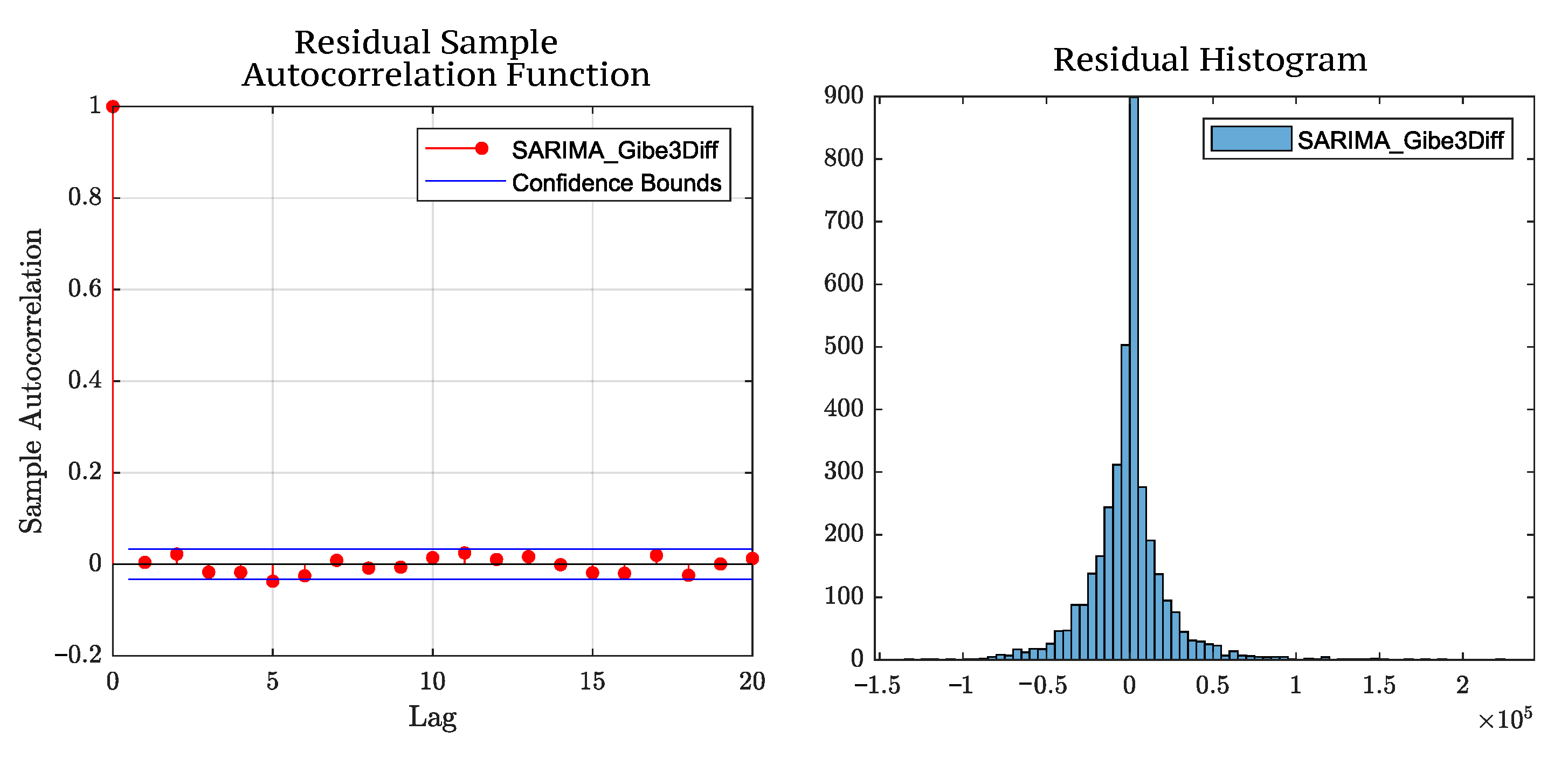
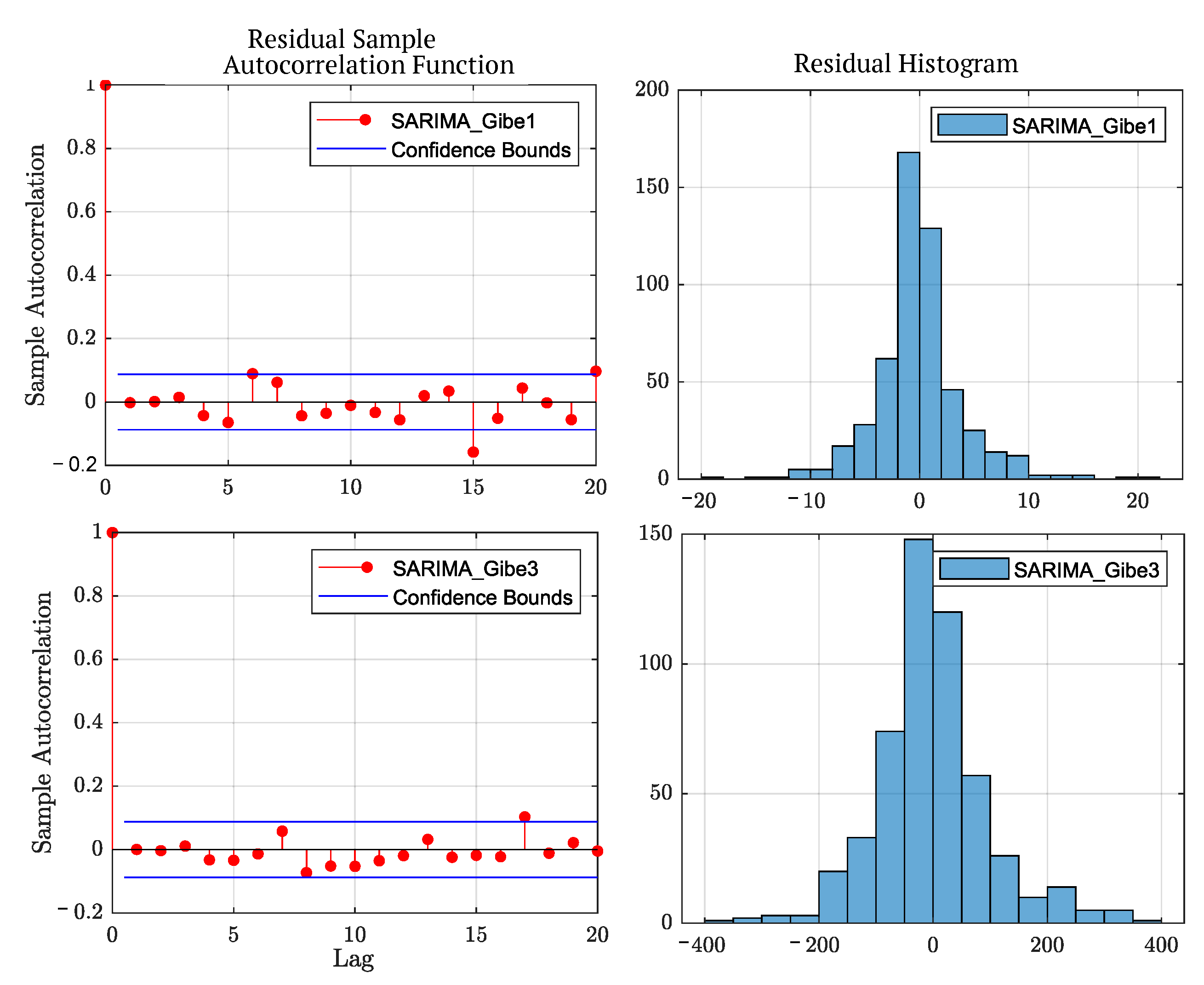
2.2.3. Residual Diagnosis
After the time series analysis and estimation of the stochastic model, there is a need to perform a residual diagnosis to make sure that the model fits the synthetic series. The property expected from a good fit is to have uncorrelated residuals with zero means [18]. In addition to these properties, having residuals with zero variance and normal distribution indicates a good model fit. We can test those properties by visually inspecting the autocorrelation function (ACF) and histogram plots of the residuals or applying various test methods. The test method proposed by [17,18] is the portmanteau test, which tests whether the first K autocorrelation is significantly different from what would be expected from a white noise process. The most used test method and the modified version of the portmanteau test is the Ljung–Box Q-test, which is incorporated in the Matlab Econometric Modeler tool based on the equitation,
The modified statistic has, approximately, the mean of the distribution [17]. This modified form of the portmanteau test statistic has been recommended for use because it has a null distribution much closer to the distribution for typical sample sizes n.
Daily Time Resolution
A residual diagnosis is performed first using a visual inspection of the ACF and Histogram plots are shown in Figure 5, which shows normally distributed and uncorrelated residuals. In addition to the visual inspection of the ACF plot, we run the Ljung–Box Q-test (LBQ) for autocorrelation of the Gibe 3 SARIMA model using the Matlab econometric modeler tool Version 5.1 (R2018b) with the test parameters of , degree of freedom , and significance level .
The null hypothesis is that the first m autocorrelation of the residuals of the SARIMA model are jointly zero.
Weekly Time Resolution
The residuals are diagnosed visually using ACF and histogram plots and the LBQ test. The results from the visual inspection of the ACF and histogram plots of the residuals in Figure 6 indicate almost normally distributed residuals without correlation. Furthermore, the results of the null hypothesis in the LBQ test with the test parameter of , the degree of freedom , and significance level show that the first m autocorrelations of the residuals of the SARIMA model are jointly zero, and the hypothesis is not rejected for both Gibe 1 and Gibe 3; the same holds for the rest of the reservoirs. That means the model passes all of the diagnosis checks, which indicates a good fit for the model.
3. Result and Discussion
This section discusses the results of the study based on the steps followed in the methodology. The objectives of this study are to derive the synthetic historical inflow time series, perform time series analysis, and estimate the stochastic model that best fits the synthetic series and generate realistic inflow scenarios that can be used in hydropower planning models.
3.1. Synthetic Historical Inflow Time Series
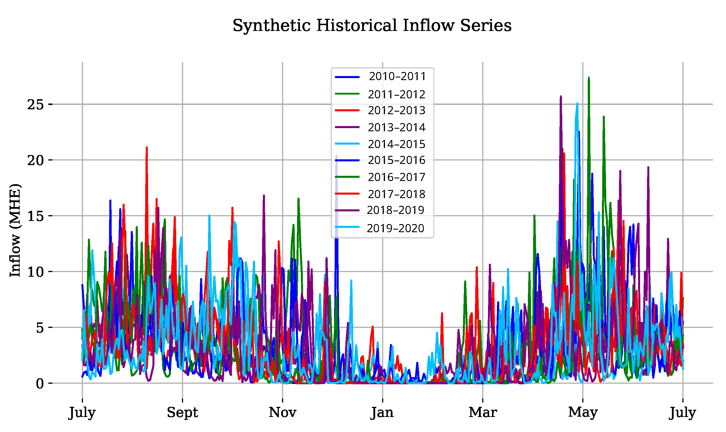
The synthetic historical inflow time series for the past ten years, from 1 July 2010 to 30 June 2020, is derived in a daily time resolution for each reservoir. Figure 7 shows the aggregate inflow time series of all the reservoirs per year in a daily time resolution.
As can be seen from the figure, there are seasonal variations in the inflows. Most of the reservoirs obtain a considerable inflow during the same season. The reservoirs’ geographical location variations create slightly different precipitation patterns.
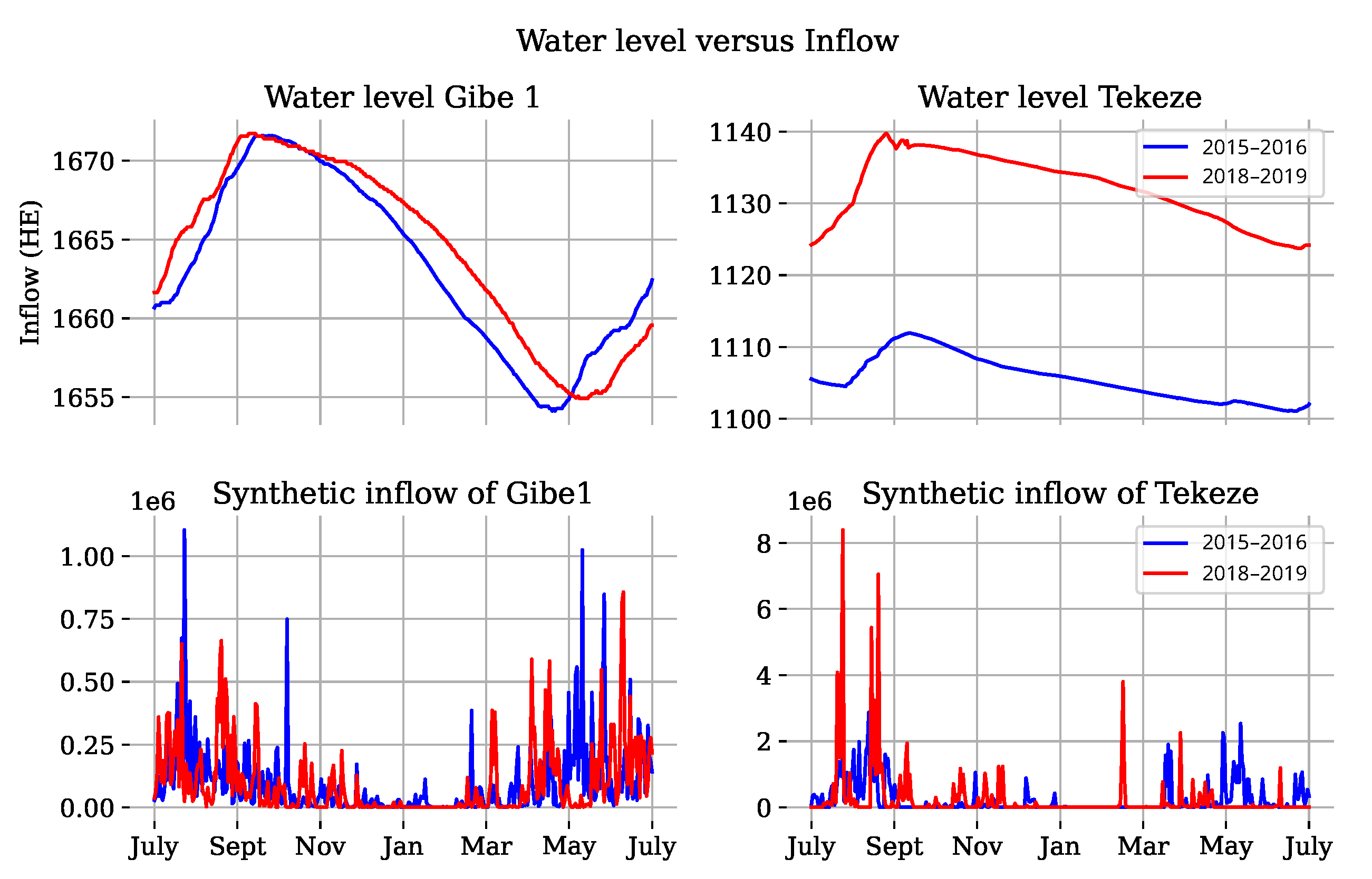
In general, all reservoirs obtain considerable rain in the rainy season, July–September, and attain their maximum levels around September and October. When we compare the actual water level, and the synthetic inflows for Gibe 1 and Tekezé reservoirs using historical water levels and synthetic inflows for 2015–2016 and 2018–2019, as shown in Figure 8, the water levels of Gibe 1 in 2015–2016 and 2018–2019 have almost similar patterns. The maximum level is at the beginning of September for both years, and it starts dropping from October throughout the dry season; the water level reaches its lowest point around April for 2015–2016 and around mid-may for 2018–2019. After that, the level starts rising relatively fast, starting from the end of April on the blue curve and rising relatively slowly from June on the red curve. It can be seen from the same figure that there is a high inflow from July to October in both years, and the inflow starts to lower from November, with very little inflow in the dry seasons in both years. In the dry season, the inflow was better in 2018–2019 than in 2015–2016. However, at the end of the planning year, i.e., from May to June, we saw a higher inflow in 2015–2016 than in 2018–2019, which corresponds to the water level pattern of each year.
The Tekezé reservoir water level for 2015–2016 and 2018–2019 in Figure 8 have similar patterns but there are big differences in water levels between the two years. When we compare the increase in the water level from July to September and the inflow for the same time, we can see that In 2015–2016 (blue curve), the level increase is only around 6 m.a.s.l, which corresponds to the lower inflow. On the other hand, in 2018–2019 (the red curve), the level increase is around 15 m.a.s.l during the same time, which corresponds to the higher inflow. Therefore, the inflow can justify the variation of the water levels for the two different years; in 2018–2019, the Tekezé reservoir had the highest rainfall in August and September and a small inflow throughout the dry season. On the other hand, in 2015–2016, the year started with a low water level, and it had lower inflow during the wet and dry seasons.
Water levels and inflows varied in a logical pattern in the two reservoirs, which held for the rest of the reservoirs, implying that the generated time series are realistic. Therefore, we can further analyze the developed inflow time series to estimate the stochastic process and generate a random but realistic inflow scenario.
3.2. Scenario Generation
We simulate sample realizations of random scenarios from the estimated SARIMA models, applying the Monte Carlo simulation using the synthetic time series and the inferred residuals as pre-sample data. Fifty different paths for two years of observation were generated for both time resolutions.
3.2.1. Daily Time Resolution
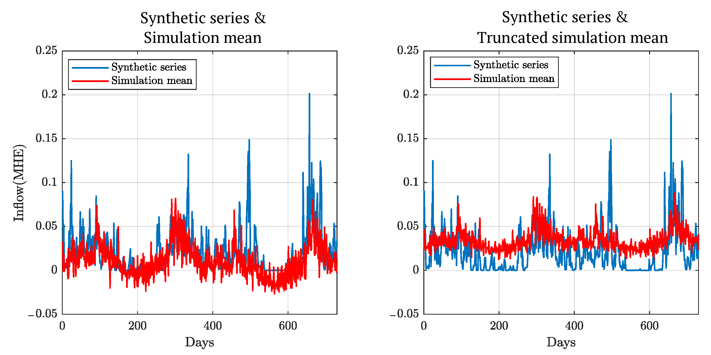
The simulation results in Figure 6 on the left-hand side show that the model captures the seasonal variation of the inflow series and follows the same pattern as the synthetic time series. It can be noted that the simulation does not have the large peaks seen in the synthetic time series. Moreover, the simulation mean goes down to the negative value when the synthetic inflow is at its minimum; this means there are negative inflows during specific periods, even if there is no negative inflow in the synthetic series. It is not realistic to have negative values for the inflow scenario. These unrealistic results are mainly due to the assumption of a Gaussian distribution in the ARIMA model estimation and the Monte Carlo sample values in the range of ( to ). Therefore, we removed the negative values from the generated scenarios by truncating the negative values to zero. The right-hand side of Figure 9 shows the synthetic time series and the mean of truncated inflow scenarios; when we compare the two curves, the simulation mean tends to the positive trough out the time of simulation because the truncation process significantly affects the simulation mean.
We can conclude that the sample realizations of the random series generated from the daily time resolution are not realistic scenarios and would not transform the features in the synthetic series to a random, future scenario.
3.2.2. Weekly Time Resolution
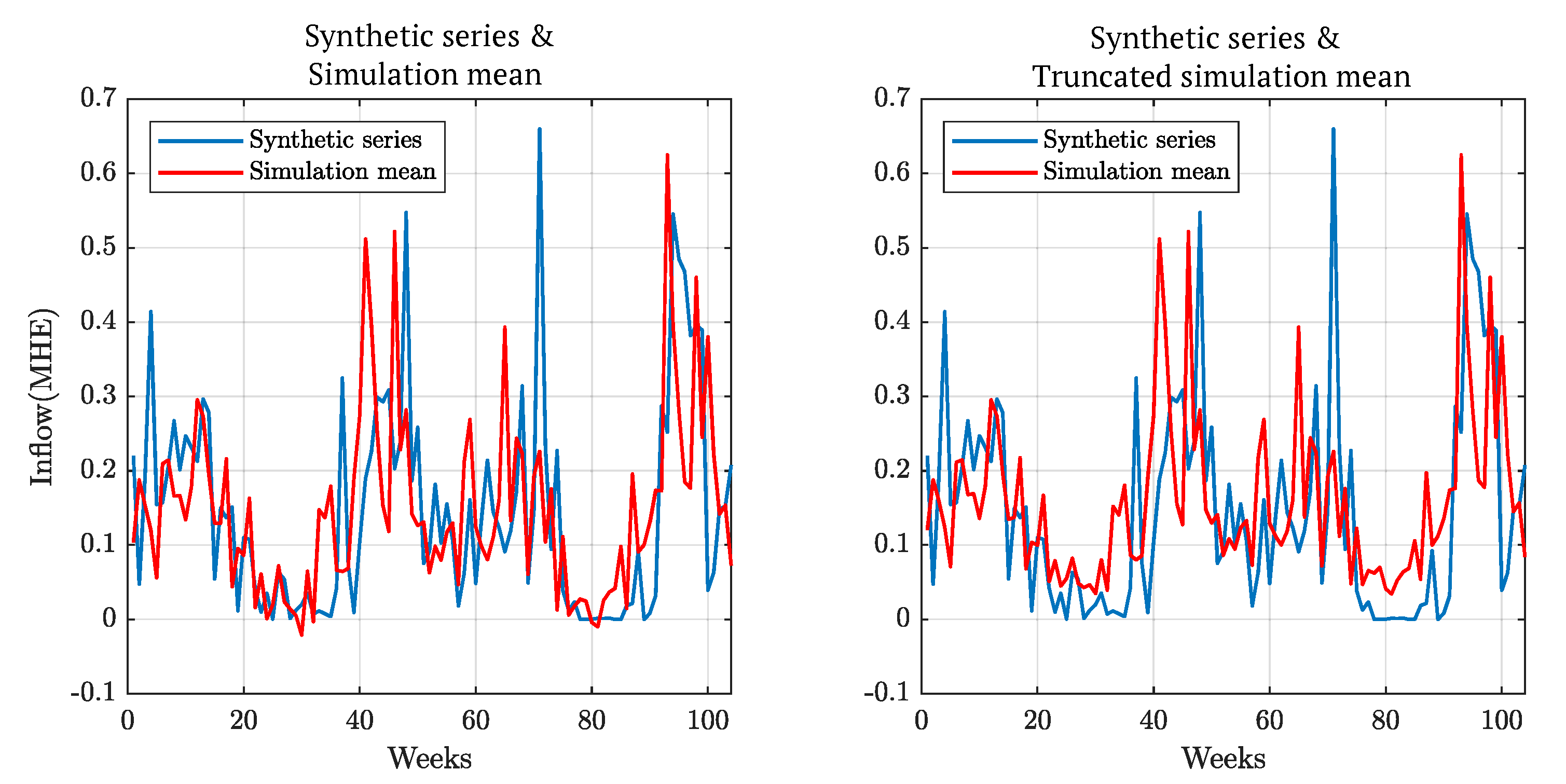
The simulation result in Figure 10 on the left-hand side shows that the simulation mean has an almost similar pattern to the synthetic series. There are two points where the mean becomes negative, indicating the presence of a negative inflow in the generated series. The figure on the right-hand side shows the synthetic series with the mean of the truncated inflow series; the result shows a slight upward shift in the simulation mean. However, the approximation effect is much less for the series in the weekly time resolution.
When we compare the simulation mean of the two data sets, in Figure 9 and Figure 10, we can see that the model in the weekly time series best captures the behavior of the synthetic time series; moreover, the effect of the truncation is less visible in the weekly resolution. Therefore we can conclude that the scenarios generated from the weekly resolution time series best capture the features in the synthetic historical series.
3.3. Evaluation of the Generated Inflow Scenarios
Random inflow scenarios could be used for long-term hydropower planning using stochastic models; however, this is beyond the scope of this paper. To verify that the scenarios are useful as inputs for hydropower planning problems, they will be tested in a deterministic model presented in [14]. The deterministic simulation model is a model used to maximize the value of stored water and minimize load shedding by utilizing the water stored in the rainy season throughout the dry season with optimized water management. The objective here is to simulate the model with the random inflow realizations and see if we can obtain a reasonable generation scheduling, acceptable load shedding, realistic reservoir level patterns, and realistic spillage compared to the actual operation in the Ethiopian power system.
Fifty scenarios have been created using the model with weekly time resolution. In case 1, the inflow is equal to the mean of all these scenarios; case 2 uses the scenario with the highest total inflow, and case 3 uses the scenario with the lowest total inflow. A load demand equal to the actual demand in 2018–2019 is considered for all of the simulations. The simulation results from the three cases are compared to the actual planning of the Ethiopian power system in 2018–2019.
The three cases of inflow scenarios and the synthetic inflow in the 2018–2019 planning year in the weekly time resolution are shown in Figure 11.
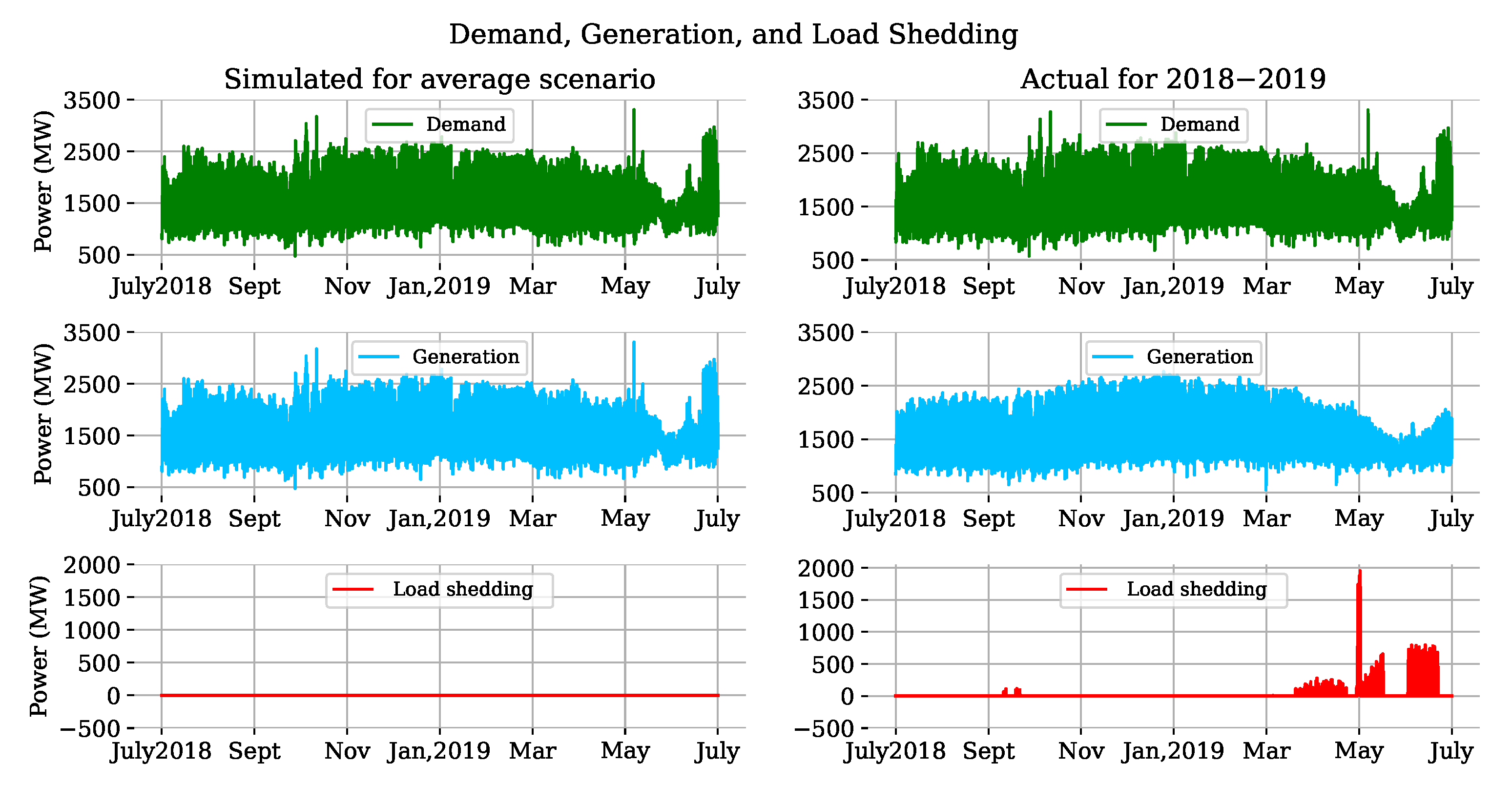
The deterministic hydropower model uses a time resolution of one hour. Therefore the inflows in weekly time resolution shown in Figure 11 are converted to hourly resolution so that any hour is assumed to be 1/168 of the corresponding weekly inflow. Figure 12 shows the comparison between the simulation results of generation and load shedding for case 1 and the actual operation in the 2018–2019 planning year, respectively.
The simulation result for the generation and load shedding shows that the model supplies the demanded load with zero load shedding. However, load shedding is observed when there is higher load demand around October and toward the end of the year in the actual operation.
The actual hydropower operation in the Ethiopian power system depends on each reservoir’s historical generation and historical water level trends. In contrast, the model will distribute generation arbitrarily between hydropower plants as long as no reservoir limits are exceeded.
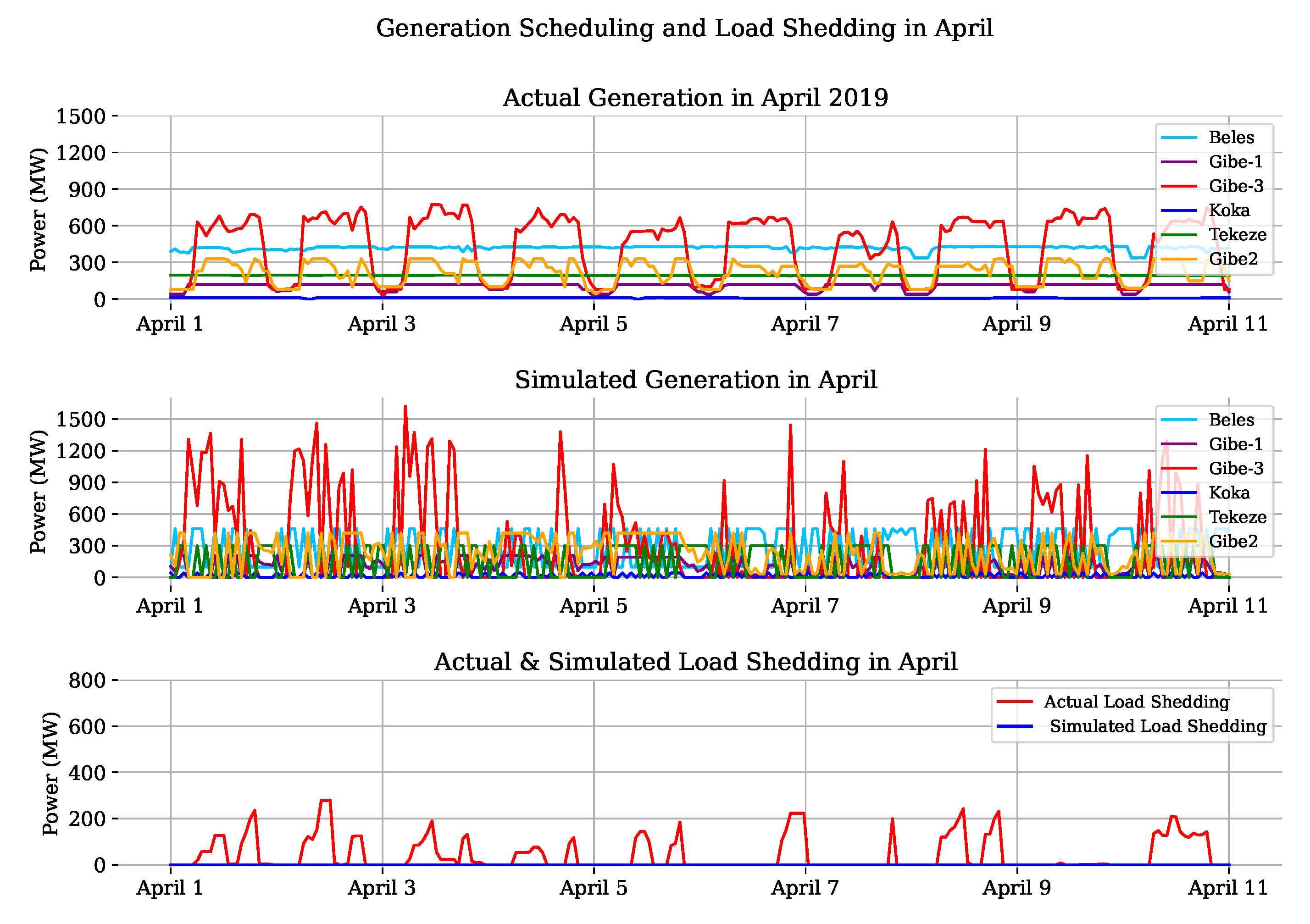
Figure 13 shows the generation scheduling in the actual and simulated operation for ten days in April, when we can see a load shedding in the actual operation and zero load shedding in the simulation.
The figure shows that the actual operation follows the same generation pattern each day, the Gibe 3 reservoir supplies the variation in the load, and the smaller reservoirs have the same generation level; consequently, we see a lot of load shedding during this time of the planning year. However, the model is expected to perform better than the actual operation since it has the perfect information. Therefore, the model schedules the generation arbitrarily between the reservoirs in the simulation to minimize load shedding and maximize stored water.
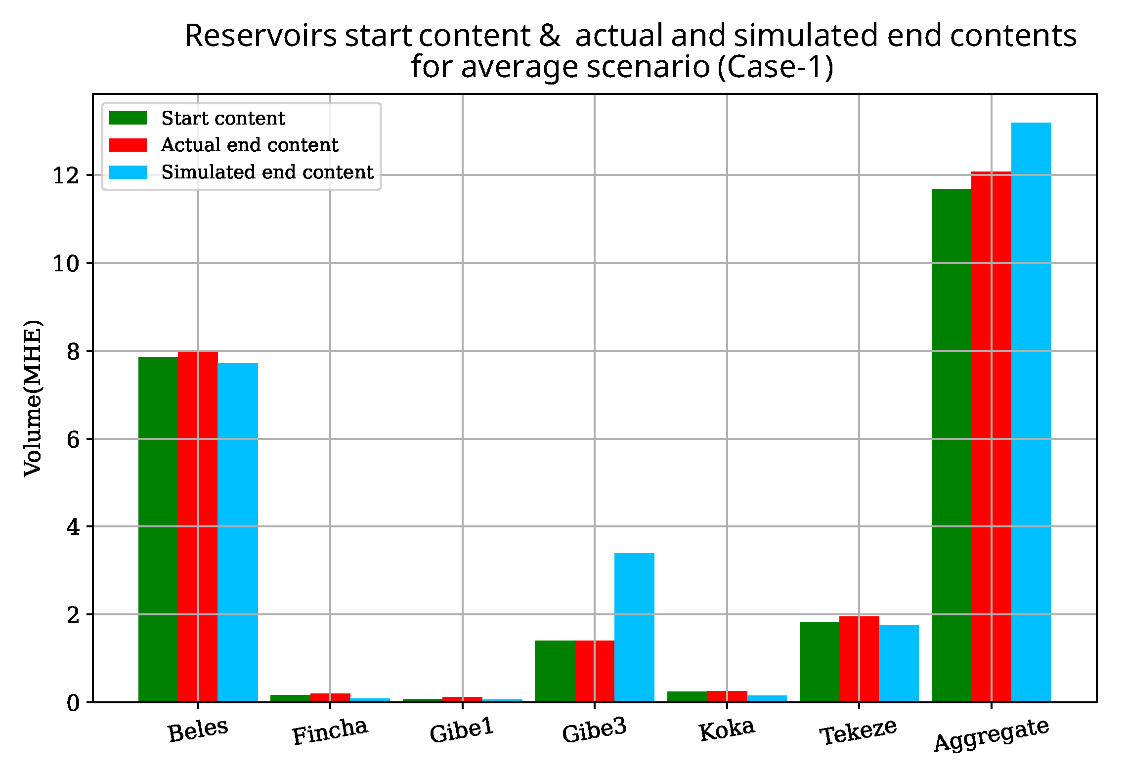
In Figure 14, we can see sample reservoirs’ start and final content for actual and simulated operations, which are at the same levels for most reservoirs except the Gibe 3 reservoir. Let us compare the synthetic historical inflow and the inflow scenario. The inflow is slightly higher in the average scenario (12.17 million HE compared to 11.15 million HE in the synthetic scenario for 2018–2019). However, on the other hand, the amount of stored water is around 1.1 million HE higher in the simulated operation of the average scenario compared to the actual operation in 2018–2019. This indicates that the load shedding in 2018–2019 was not because there was insufficient water but because the water was not used efficiently. In practice, water must have been spilled during the earlier rainy seasons. Unfortunately, there are no records of spillage from Ethiopian hydropower plants which can confirm this conclusion.
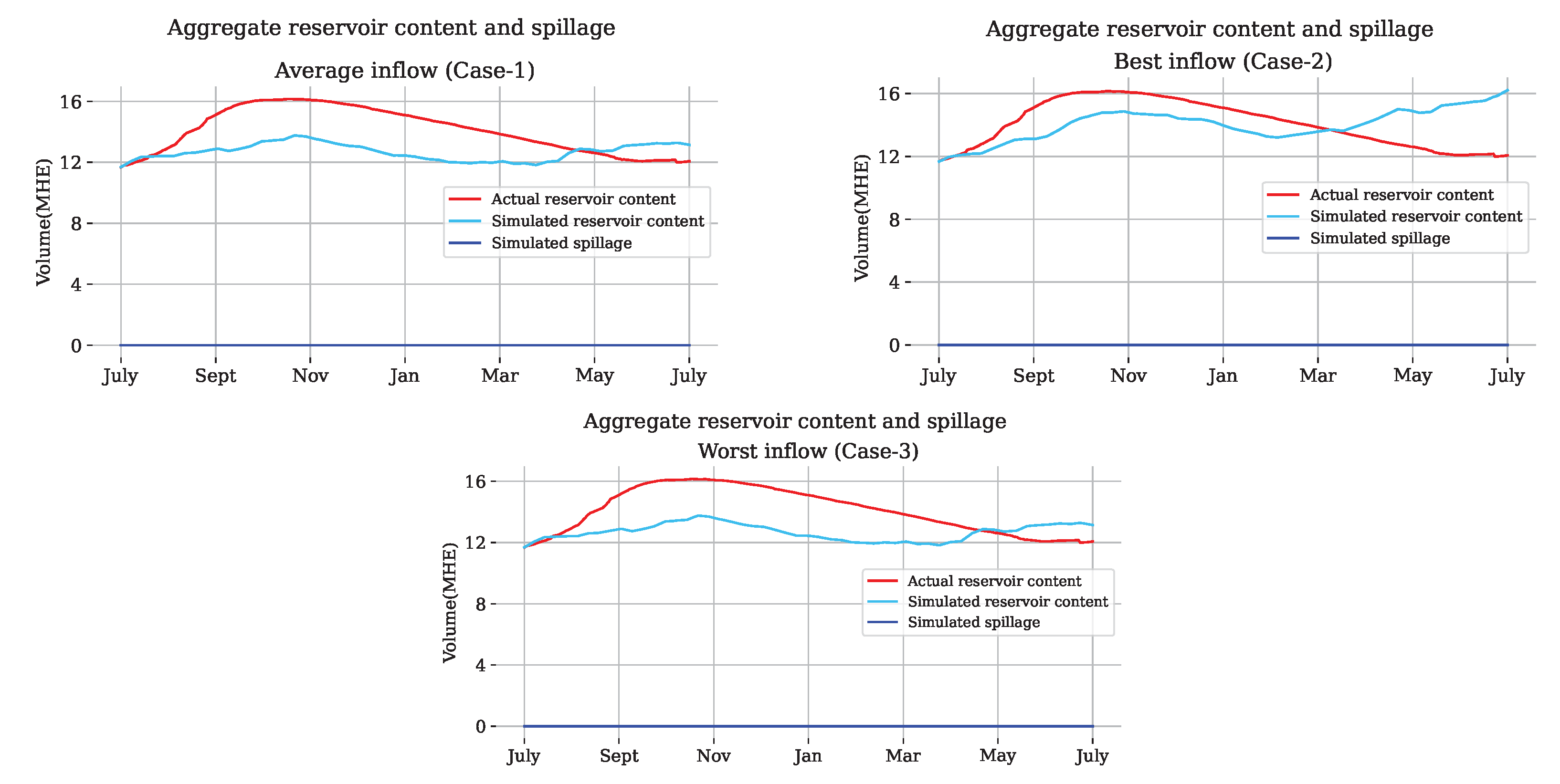
If the inflow scenarios were unrealistic, we could, for example, have periods with full reservoirs (due to inflow peaks) and spillage, or we could have periods with empty reservoirs and plenty of load shedding. However, no such problems are experienced in the simulation of all three cases, as presented in Figure 15. The figure shows the aggregate reservoir contents in the actual and simulation of the three cases and the corresponding simulated spillage trough out the year. However, we could not compare the actual spillage in reality with the simulation result because there is no data available to compare.
Therefore, we can conclude that the random inflow scenarios generated are good enough to obtain realistic results. From a long-term perspective, it would be more efficient to use planning tools taking into account forecasts rather than the existing rules of thumb or following historical generation trends.
4. Conclusions and Recommendations
This paper presents a method to develop a synthetic historical inflow time series by combining hydropower generation data and satellite precipitation measurement. The identification of the stochastic process and inflow scenario generation is also presented. With the proposed methods, we can generate two sets of synthetic historical time series with daily and weekly time resolutions from the limited available data. We have shown that existing methods can be applied to identify the stochastic process and generate realistic inflow scenarios for the Ethiopian power system considering the limited data available. We use the Box–Jenkins family of stochastic process estimation models to perform the time series analysis and estimate the stochastic process of each reservoir. In addition, we used the seasonal ARIMA model to estimate the stochastic process and consider the seasonality of 365 for the daily resolution and 52 for the weekly resolution. We observed that, even if these data sets are extracted from the same synthetic historical time series, the time series in the daily time resolution are all non-stationary, seasonal integrated moving average stochastic processes, for example, SARIMA(0,1,2)(0,1,2)[730] for Gibe 1. On the contrary, the time series with weekly time resolutions are all stationary seasonal autoregressive processes of various orders. SARIMA(3,0,0)(3,0,0)[104] for Gibe 1.
The Monte Carlo simulation is used to generate the scenarios from the fitted stochastic models for both data sets. The simulation means from both data sets follow the synthetic historical time series pattern. However, the Gaussian assumption in the ARIMA models and the Monte Carlo sample values in the range ( to ) create a sample with negative inflow values. The problem is mitigated by truncating the negative values to zero. However, this affects the value of the simulation mean, which was significant in the daily time resolution and less significant in the weekly time resolution. Consequently, the time series with daily time resolution overestimates the inflows and misses some peak points from the synthetic series. In contrast, the time series with the weekly resolution best captures the characteristics of the synthetic historical time series and can generate realistic random scenarios. The evaluation of the inflow scenarios indicates that they are good enough to generate reasonable results.
These random inflow scenarios can be used in future works to apply stochastic planning models for hydropower in Ethiopia and other countries. Better planning tools can improve the utilization of hydropower in order to minimize generation costs and load shedding.
If Ethiopia is going to have a modern power system, a detailed hydrological model is necessary; it is not currently in place. A long-term objective to develop such a model is recommended. It could be part of future research work to compare the simplified model with what we could do if we had a detailed hydrological model. We also recommend temporal and spatial correlations in inflows for reservoirs in related locations, considering the correlation between inflow and wind speed, as there might be an expansion of wind power generation in the Ethiopian power system in the future.
Author Contributions
Conceptualization, F.G.D. and M.A.; formal analysis, F.G.D.; investigation, F.G.D.; methodology, F.G.D. and M.A.; project administration, M.A. and G.B.; software, F.G.D.; supervision, M.A. and G.B.; validation, F.G.D.; writing—review and editing, F.G.D., M.A., and G.B. All authors have read and agreed to the published version of the manuscript.
Funding
This research was funded by the SIDA-Ethiopia Bilateral program, contribution number 51080124. The APC was funded by the KTH Royal Institute of Technology.
Institutional Review Board Statement
Not applicable.
Informed Consent Statement
Not applicable.
Data Availability Statement
The data presented in this study are available upon request from the corresponding authors.
Acknowledgments
The authors gratefully acknowledge the contributions of the Swedish International Development Cooperation Agency (SIDA) to funding this research project. The collaboration of the KTH Royal Institute of Technology, Sweden, and Addis Ababa Institute of Technology (AAIT), Ethiopia, to facilitate the project study, and the Ethiopian Electric Power (EEP), to provide the necessary data for the research work.
Conflicts of Interest
The authors declare no conflict of interest.
Abbreviations
The following abbreviations are used in this manuscript:
| ACF | autocorrelation function |
| AR | autoregressive |
| ARFIMA | autoregressive fraction integrated moving average model |
| ARIMA | autoregressive integrated moving average |
| DAV | data access viewer |
| DOF | degree of freedom |
| EEP | Ethiopian Electric power |
| GIS | geographic information systems |
| MA | moving average |
| MAE | mean annual energy |
| MAI | mean annual inflow |
| NEXRA | Next Generation Weather Radar |
| PAR | periodic autoregressive |
| PARMA | periodic autoregressive-moving average |
| PRMS | precipitation-runoff modeling system |
| SARIM | seasonal autoregressive integrated moving average model |
| SDDP | stochastic dual dynamic programming |
| SWAT | surface water assessment tool |
References
- International Hydropower Association. 2022 Hydropower Status Report; Hydropower.org: Lodon, UK, 2022. [Google Scholar]
- Daniel, E.B. Watershed Modeling and its Applications: A State-of-the-Art Review. Open Hydrol. J. 2011, 5, 26–50. [Google Scholar] [CrossRef] [Green Version]
- Markstrom, S.L.; Regan, R.S.; Hay, L.E.; Viger, R.J.; Webb, R.M.T.; Payn, R.A.; LaFontaine, J.H. 2015, PRMS-IV, the Precipitation-Runoff Modeling System Version IV; U.S. Geological Survey Techniques and Methods: Lakewood, CO, USA, 2015; book 6, chap. B7; 158p. [Google Scholar]
- Teng, F.; Huang, W.; Cai, Y.; Zheng, C.; Zou, S. Application of hydrological model PRMS to simulate daily rainfall runoff in Zamask–Yingluoxia subbasin of the Heihe River Basin. Water 2017, 9, 769. [Google Scholar] [CrossRef] [Green Version]
- Daniel, E.B.; Camp, J.V.; Leboeuf, E.J.; Penrod, J.R.; Abkowitz, M.D.; Dobbins, J.P. Watershed Modeling Using GIS Technology: A Critical Review. J. Spat. Hydrol. 2010, 10, 14–28. [Google Scholar]
- Moon, J.; Srinivasan, R.; Jacobs, J.H. Stream flow estimation using spatially distributed rainfall in the Trinity River basin, Texas. Trans. ASAE 2004, 47, 1445–1451. [Google Scholar] [CrossRef]
- Obeysekera, J.T.; Salas, J.D. Modeling of aggregated hydrologic time series. J. Hydrol. 1986, 86, 197–219. [Google Scholar] [CrossRef]
- Stokelj, T.; Paravan, D.; Golob, R. Short and mid term hydro power plant reservoir inflow forecasting. In Proceedings of the PowerCon 2000—2000 International Conference on Power System Technology, Perth, Australia, 4–7 December 2000; IEEE: Piscataway, NJ, USA, 2000; Volume 2, pp. 1107–1112. [Google Scholar] [CrossRef]
- Sharma, A.; O’Neill, R. A nonparametric approach for representing interannual dependence in monthly streamflow sequences. Water Resour. Res. 2002, 38, 5-1–5-10. [Google Scholar] [CrossRef]
- Jimenez, C.; Mcleod, A.I.; Hipel, K.W. Stochastic Hydrology and Hydraulics Kalman filter estimation for periodic autoregressive-moving average models. In Stochastic Hydrology and Hydraulics; Springer: Berlin/Heidelberg, Germany, 1989; Volume 3, pp. 227–240. [Google Scholar]
- Pereira, G.; Veiga, A. PAR(p)-vine copula based model for stochastic streamflow scenario generation. Stoch. Environ. Res. Risk Assess. 2018, 32, 833–842. [Google Scholar] [CrossRef]
- Wang, W.; Dong, Z.; Zhu, F.; Cao, Q.; Chen, J.; Yu, X. A stochastic simulation model for monthly river flow in dry season. Water 2018, 10, 1654. [Google Scholar] [CrossRef] [Green Version]
- De Almeida Pereira, G.A.; Souza, R.C. Long Memory Models to Generate Synthetic Hydrological Series. Math. Probl. Eng. 2014, 2014, 823046. [Google Scholar] [CrossRef]
- Dires, F.G.; Amelin, M.; Bekele, G. Deterministic Hydropower Simulation Model for Ethiopia. In Proceedings of the 2021 IEEE Madrid PowerTech, PowerTech 2021—Conference Proceedings, Madrid, Spain, 28 June–2 July 2021. [Google Scholar] [CrossRef]
- POWER|Data Access Viewer. Resources NASA Prediction of Worldwide Energy 2022, POWER Data Access Viewer. Available online: https://power.larc.nasa.gov/data-access-viewer/ (accessed on 19 November 2022).
- Analyze Time Series Data Using Econometric Modeler—MATLAB and Simulink—MathWorks Nordic, Help Center Documentation. Available online: https://se.mathworks.com/help/econ/econometric-modeler-overview.html (accessed on 21 November 2022).
- Box, G.E.P.; Jenkins, G.M.; Reinsel, G.C. Time Series Analysis; Wiley Series in Probability and Statistics; Wiley: Hoboken, NJ, USA, 2008; pp. 1–746. [Google Scholar] [CrossRef]
- Hyndman, R.J. George Athanasopoulos. 3.3 Residual Diagnostics|Forecasting: Principles and Practice, 2nd ed.; OTexts: Melbourne, Australia, 2018. [Google Scholar]
Figure 1.
Map of Ethiopian Hydropower stations.

Figure 2.
Historical pattern of water levels for Gibe 1, Gibe 3, Koka, and Tekezé reservoirs; source: EEP.
Figure 2.
Historical pattern of water levels for Gibe 1, Gibe 3, Koka, and Tekezé reservoirs; source: EEP.

Figure 3.
Methodology framework.

Figure 4.
Model −1 fit for the Gibe 1 and Gibe 3 time series in the weekly time resolution.

Figure 5.
Residual diagnosis of the differenced Gibe 3 time series.

Figure 6.
Residual diagnosis of the weekly time resolution.

Figure 7.
Synthetic historical inflow time series plot for the Ethiopian power system.

Figure 8.
Actual water level versus synthetic inflow in 2015–2016 and 2018–2019 for Gibe 1 and Tekezé reservoirs.
Figure 8.
Actual water level versus synthetic inflow in 2015–2016 and 2018–2019 for Gibe 1 and Tekezé reservoirs.

Figure 9.
Simulation mean and synthetic historical series for Gibe 3 in the daily time resolution.

Figure 10.
Simulation mean and synthetic historical series in the weekly resolution.

Figure 11.
The three cases of inflow scenarios and synthetic inflow of 2018–2019.

Figure 12.
Simulation results for case 1 and actual operation 2018–2019 planning year.

Figure 13.
Actual and simulated load shedding and generation schedule for sample reservoirs in April.
Figure 13.
Actual and simulated load shedding and generation schedule for sample reservoirs in April.

Figure 14.
Start and final reservoir contents for the actual operation and simulation of case 1.

Figure 15.
Actual reservoir content plus simulated reservoir content and spillage for the tree cases.
Figure 15.
Actual reservoir content plus simulated reservoir content and spillage for the tree cases.


Table 1.
Reservoir generation information and geographical location.
| Power Plant | Coordinates °N, °E | Dam Height (m) | Maximum Level (m a.s.l) | Storage (Mm3) at Max. Level | Installed Capacity (MW) | Maximum Discharge (m3/s) | Average Energy (GWH) |
|---|---|---|---|---|---|---|---|
| Beles | 11.82, 36.92 | 35.00 | 1787.00 | 37,307.00 | 460.00 | 160.00 | 1867.00 |
| M.Wakena | 7.225, 39.462 | 42.00 | 2522.90 | 875.00 | 153.00 | 60.00 | 543.00 |
| Fincha | 9.789, 37.269 | 22.20 | 2219.00 | 964.00 | 134.00 | 29.68 | 760.00 |
| Gibe I | 7.831, 37.322 | 41.00 | 1,671.55 | 863.00 | 210.00 | 100.00 | 722.00 |
| Gibe II | 7.757, 37.562 | 46.50 | Diversion Weir | - | 420.00 | 98.12 | 1635.00 |
| Gibe III | 6.844, 37.301 | 243.00 | 892.00 | 15,500.00 | 1870.00 | 2200.00 | 6500.00 |
| Koka | 8.468, 39.156 | 23.80 | 1599.00 | 4250.00 | 42.00 | 144.00 | 110.00 |
| Awash II | 8.468, 39.156 | river | run-of-river | - | 32.00 | 65.60 | 182.00 |
| Awash III | 8.468, 39.156 | river | run-of-river | - | 32.00 | 66.20 | 182.00 |
| Tekezé | 13.348, 38.742 | 188.00 | 1140.10 | 9310.00 | 300.00 | 184.00 | 1393.00 |
| Am. Neshe | 9.789, 37.269 | 38.00 | 2232.50 | 526.10 | 97.00 | 18.70 | 35.00 |
| Tis Abay I | 11.486, 37.587 | river | run-of-river | - | 12.00 | 114.00 | 33.70 |
| Tis Abay II | 11.486, 37.587 | river | run-of-river | - | 72.00 | 114.00 | 359.00 |
Source: EEP.
Table 2.
Test results.
| Null Rejected | p-Value | Test Statistic | Critical Value | |
|---|---|---|---|---|
| 1 | false | 0.27408 | 23.3047 | 31.4104 |
Table 3.
Model estimation results for SARIMA(0,1,3)(0,1,2)[365] Model.
| Parameter | Value | Standard Error | T Statistic | p Value |
|---|---|---|---|---|
| Constant | 0 | 0 | ||
| MA{1} = | −1.403 | 0.045174 | −31.0574 | 9.0611 |
| MA{2} = | 0.28348 | 0.085036 | 3.3336 | 0.00085725 |
| MA{3} = | 0.1482 | 0.058094 | 2.551 | 0.010741 |
| SMA{1} = | −0.77234 | 0.064318 | −12.0081 | 3.2218 |
| SMA{2} = | 0.014517 | 0.070344 | 0.20637 | 0.8365 |
| Variance | 3.0546 | 3.1855 | 9.5891 | 0 |
Disclaimer/Publisher’s Note: The statements, opinions and data contained in all publications are solely those of the individual author(s) and contributor(s) and not of MDPI and/or the editor(s). MDPI and/or the editor(s) disclaim responsibility for any injury to people or property resulting from any ideas, methods, instructions or products referred to in the content. |
© 2023 by the authors. Licensee MDPI, Basel, Switzerland. This article is an open access article distributed under the terms and conditions of the Creative Commons Attribution (CC BY) license (https://creativecommons.org/licenses/by/4.0/).
Share and Cite
MDPI and ACS Style
Dires, F.G.; Amelin, M.; Bekele, G. Inflow Scenario Generation for the Ethiopian Hydropower System. Water 2023, 15, 500. https://doi.org/10.3390/w15030500
AMA Style
Dires FG, Amelin M, Bekele G. Inflow Scenario Generation for the Ethiopian Hydropower System. Water. 2023; 15(3):500. https://doi.org/10.3390/w15030500
Chicago/Turabian StyleDires, Firehiwot Girma, Mikael Amelin, and Getachew Bekele. 2023. "Inflow Scenario Generation for the Ethiopian Hydropower System" Water 15, no. 3: 500. https://doi.org/10.3390/w15030500
Note that from the first issue of 2016, this journal uses article numbers instead of page numbers. See further details here.