
Intercomparing LSTM and RNN to a Conceptual Hydrological Model for a Low-Land River with a Focus on the Flow Duration Curve

1
Research and Transfer, Jade University of Applied Sciences Wilhelmshaven/Oldenburg/Elsfleth, 26121 Oldenburg, Germany
2
Physical Geography, Department of Spatial and Environmental Science, Trier University, 54296 Trier, Germany
*
Author to whom correspondence should be addressed.
Water 2023, 15(3), 505; https://doi.org/10.3390/w15030505
Submission received: 20 December 2022
/
Revised: 13 January 2023
/
Accepted: 22 January 2023
/
Published: 27 January 2023
(This article belongs to the Special Issue The Application of Artificial Intelligence in Hydrology, Volume II)
Abstract
:Machine learning (ML) algorithms slowly establish acceptance for the purpose of streamflow modelling within the hydrological community. Yet, generally valid statements about the modelling behavior of the ML models remain vague due to the uniqueness of catchment areas. We compared two ML models, RNN and LSTM, to the conceptual hydrological model Hydrologiska Byråns Vattenbalansavdelning (HBV) within the low-land Ems catchment in Germany. Furthermore, we implemented a simple routing routine in the ML models and used simulated upstream streamflow as forcing data to test whether the individual model errors accumulate. The ML models have a superior model performance compared to the HBV model for a wide range of statistical performance indices. Yet, the ML models show a performance decline for low-flows in two of the sub-catchments. Signature indices sampling the flow duration curve reveal that the ML models in our study provide a good representation of the water balance, whereas the HBV model instead has its strength in the reproduction of streamflow dynamics. Regarding the applied routing routine in the ML models, there are no strong indications of an increasing error rising upstream to downstream throughout the sub-catchments.
Keywords:
river discharge; streamflow; LSTM; RNN; HBV model; model intercomparison; flow duration curve1. Introduction
Conceptual and process-based models are the traditional way to represent catchment hydrological processes. Based on process understanding, equations are combined to mimic the observed flow processes. The Hydrologiska Byråns Vattenbalansavdelning (HBV) model is one of the pioneers of catchments’ hydrological models [1,2]. It was applied in numerous catchments around the world, representing water flow of catchments with different characteristics. However, despite the plausible hydrological behavior, such models are limited by the understanding of the underlying processes, limiting the models’ flexibility to represent catchments’ individual flow processes. The underlying uncertainties resulting from those limitations have been widely discussed [3,4].
Next to conceptual and physical hydrological models, also, data-driven approaches such as machine learning (ML) and Deep Learning (DL) gained awareness in the scientific community due to data availability and rising computational power. Whereas conceptional models and physical models rely on our, so far, acquired knowledge about the hydrological cycle, instead, ML models are purely based on observations and do not require information about the physical properties [5]. ML models mimic the physical, relevant runoff processes from historical data by building functional relationships between input and output data [6]. The rapid progress of ML is arguably even one of the most important advances in hydrology in recent years [7].
Numerous approaches of different ML models were applied in hydrology in the past, using, for example, Artificial Neural Networks (ANNs) [8,9,10] or Support Vector Machines (SVMs) [11,12]. However, during recent years, DL models with a recurrent design such as Long Short-Term Memory (LSTM) models have been predominately applied to forecast streamflow within ML [13,14,15,16,17]. Moreover, in other environmental disciplines, such as groundwater modelling, air pollution modelling and climate change forecasting, LSTM have gained rising attention due to their superior performance for the prediction of sequential data and modelling of long-term dependencies [18,19,20,21,22].
In general, recent hydrological research often focus on multi-catchment modeling to gain generally valid results [23]. However, river flow processes are influenced by basin-specific factors, and models tend to perform unequally well for low-, medium-, and high-flow zones [24]. Specific approaches might be required in catchments where the effects of groundwater flow dominate [25]. Therefore, we (i) compared the results of a conceptual model (HBV) to two recurrent ML models (i.e., Recurrent Neural Network (RNN), LSTM) for the mainly baseflow-influenced river Ems in northwestern Germany. We used a wide range of statistical performance indices but also included metrics focusing on specific parts of the flow duration curve (FDC) to gain an in-depth understanding of the model performance. Furthermore, (ii) we applied a simple routing routine for the individual sub-catchments in the catchment and tested whether modelled upstream inflow works sufficiently as forcing data for ML models or whether error is adding up upstream-to-downstream.
2. Materials and Methods
2.1. Study Area
The Ems catchment area covers a total area of around 17,800 km2 within northwestern Germany and the Netherlands. The river flows 371 km from its spring to the outlet in the Northern Sea with a relatively low elevation difference of only 135 m and a general flow direction from southeast to northwest. The catchment’s climate is defined by the humid–temperate western wind zone of Central Europe with pronounced, but not very long, cold seasons. Mild winters, cool summers and abundant precipitation characterize this Atlantic-influenced region, whereas easterly wind conditions result in drier conditions, warmer summers as well as colder winters. Mean long-term annual precipitation is about 800 mm; mean annual temperature is between 8.5, and 9 °C and mean annual potential evapotranspiration (pET) is around 490 mm. The discharge of the Ems in most years is characterized by flood events in winter and a low-flow period from June to October. The high-flow phase usually lasts from December to March [26].
The spring of the Ems is located in the heathland area Senne in the federal state North Rhine–Westphalia from where it continues through the Münster chalk basin. After surpassing the last stretches of the Teutoburger Forest, the stream flows through limestone dominated geology. Sand and clay dominate the catchment’s soil, and the baseflow ratio is relatively high, up to 0.8 [27]. Downstream from the weir Herbrum, the river is influenced by the tide on the last 50 km before flowing into the Dollart, a bay-like estuary.
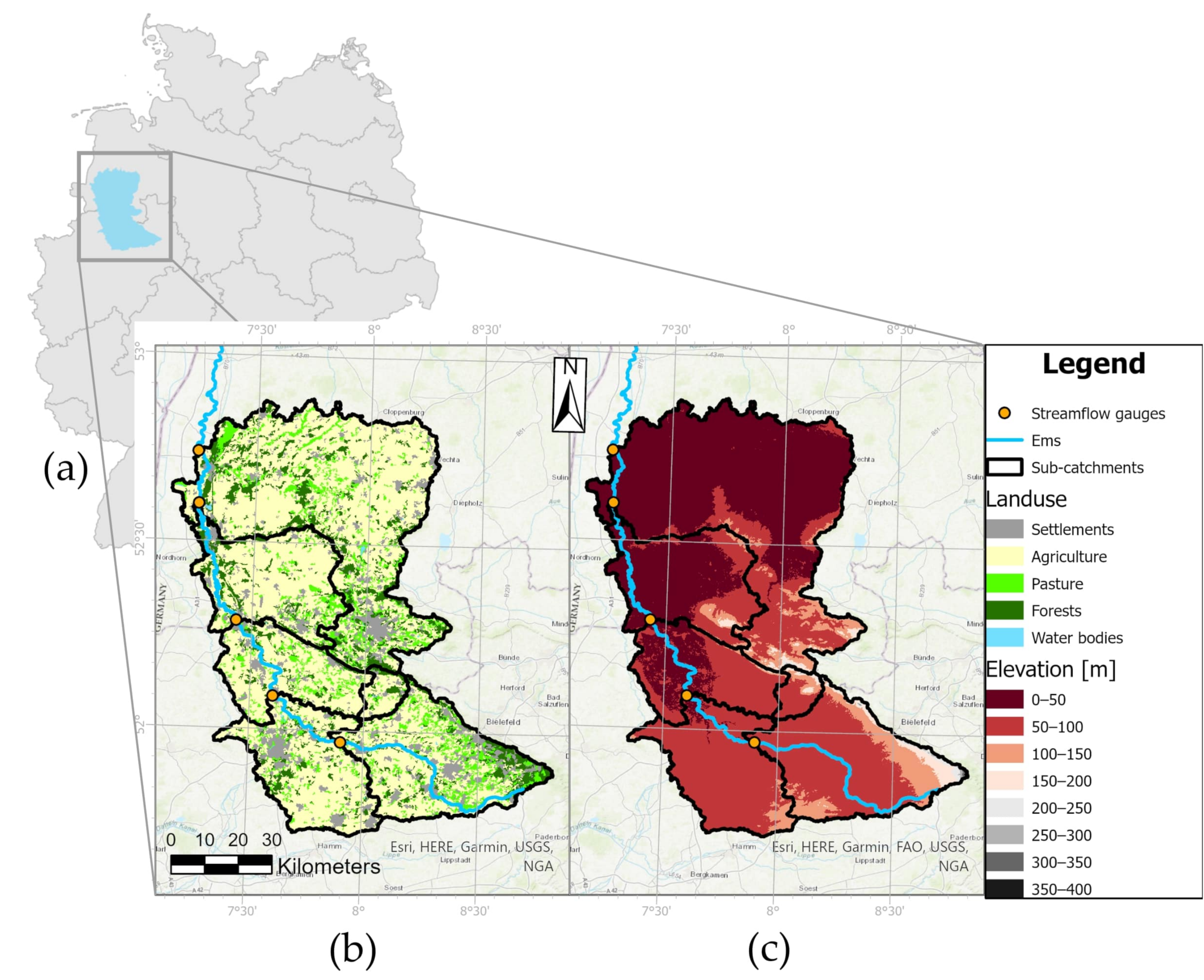
Compared to other large European catchments, the Ems can be considered rather rural, as it does not cross any major cities. Yet, about three million people live within the catchment area, and land use is characterized by intensive agriculture. The upstream part of the river is mainly covered with areas for crop production whereas the downstream area (not simulated in this study due to a lack of streamflow gauges) (Figure 1) is covered by pasture areas predominantly. Due to its far-stretched floodplains, historically, the catchment suffered regular flooding and riverbed modifications, and weirs have since controlled streamflow. Just in recent years due to the requirements in the European Water Framework Directive, local constructions have been conducted to restore the natural dynamics of the river. The river still has significant economic importance—in particular, the downstream part, which is declared a federal waterway [26].
2.2. Data
Hydro–climatic input data were obtained from the federal observation network in Germany provided in the Climate Data Center of the German Weather Service [28]. All available stations inside the official Ems catchment area were considered. Within the timeframe 1 January 1960 to 31 December 2016, the number of stations stated in Table 1 were available. They do not necessarily provide information over the whole period because stations are added to and withdrawn from the observation network on a regular basis. Data gaps were not filled. Daily mean streamflow data were acquired for five available gauges from the Global Runoff Data Center (GRDC) [29]. For each day and each variable, all available stations were used for a two-dimensional inverse distance weighting interpolation (IDW) to generate daily raster datasets to prepare the hydro–climatic input data for the specific model requirements. Then the mean values within each sub-catchment were calculated. On average, only about 60% of the stations are available for a particular day. However, potential biases due to missing data and the orographic effects on climate data can be neglected, due to the homogeneity and low elevation differences in all sub-catchments. Furthermore, Corine Land Cover data [30] were used to distinguish the dominant land use within the sub-catchments to derive a preliminary kc-value for the HBV model before calibration.
2.3. Models
2.3.1. HBV
The HBV model [1,2] is a semi-distributed conceptual rainfall–runoff model and has been previously applied in northern and central Europe, e.g., in Germany [32], Sweden [33], the Meuse river [34] and Slovakia [35]. The HBV showed a robust model performance in a model intercomparison study in central Germany compared to other hydrological catchment models [36].
Precipitation input is transferred to streamflow by a potential snow routine, soil routine, runoff and response routine, and three different reservoirs are implemented to store water within the hydrological system: soil moisture storage, upper zone storage and lower zone storage. The general water balance is defined by Equation (1):
where P is precipitation, E is evapotranspiration, Q is streamflow, SP is snow pack, SM is the soil moisture, UZ and LZ are the upper and lower ground water zone and lakes represent the volume of potential lakes [37]. For a detailed description of the model design, please refer to Bergström [2].
Forcing data requirements are precipitation, temperature and potential evapotranspiration to return streamflow at the catchment’s outlet with a daily timestep. Daily precipitation sum and daily mean temperature were directly taken from the interpolated measured data mentioned above in Table 1. Potential evaporation instead was calculated based on the approach of Haude [31].
2.3.2. RNN
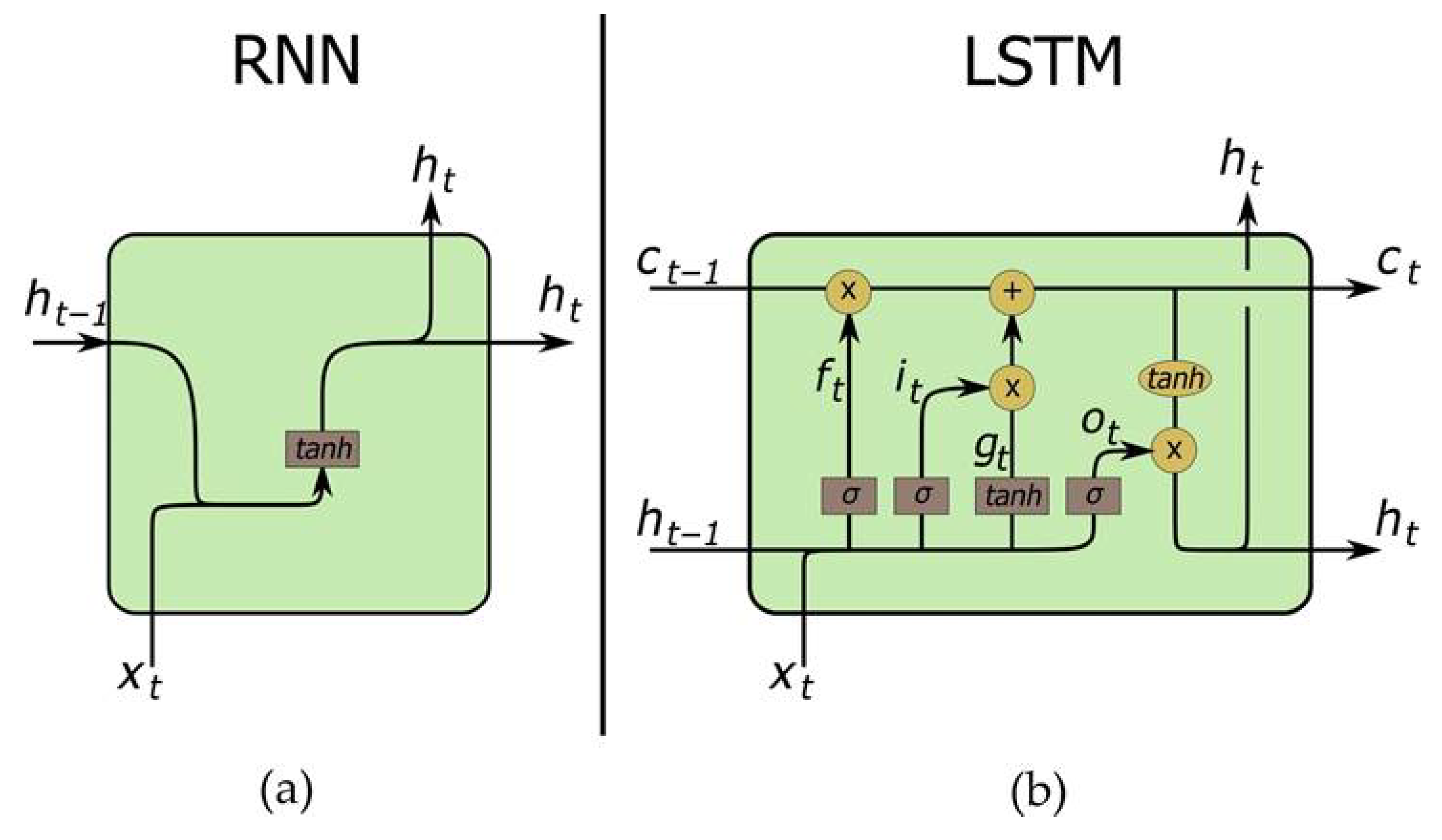
In early state machine learning architectures, the network could not “remember” past states [6], which is vital for the modeling of processes with high autocorrelation. The recurrent neural network was first introduced in the 1980s [38]. RNN cells include a feedback loop, which redirects information from the previous timestep back into the cell. That way the output from step t − 1 is transferred back into the network to influence the outcome of step t and for each subsequent step [14] (Figure 2a). RNNs are typically used for time series modeling [6]. However, Bengio et al. [39] showed that, in traditional RNN structures, a maximum of 10 timesteps is remembered by the model. In the hydrological context, this seems to be sufficient to model the response of streamflow to rainfall events induced by fast surface and sub-surface streamflow, but it does not necessarily cover long-term processes [40]. The RNN’s output is calculated by the following equation:
is the internal state/output computed within each timestep. is the hyperbolic tangent activation function, and is the input of the current timestep, whereas and are learnable parameters.
2.3.3. LSTM
With the Long Short-Term Memory, a more sophisticated recurrent design was introduced [41] (Figure 2b). Compared to other recurrent network architectures, LSTMs do not suffer from exploding or vanishing gradients. This makes them, in particular, suitable for the modelling of processes including long-term storage effects such as streamflow, which is altered by enduring dependencies such as soil moisture and snow accumulation [40]. The idea behind the LSTM is a so-called cell state, which works as the long-term memory of the cell. This cell state is fed back into the LSTM cell in the following timestep but is modified by the forget gate, which can alter the cell state. The internal processes within the LSTM cell can be described by the following equations [13]:
Referring to Figure 2b,, and are the input gate, forget gate and output gate. is the cell input; is the forcing data input at timestep , and is the hidden-state of the previous timestep. is the cell state of the previous timestep. and are adjustable parameters during the training process, while the subscripts indicate for which gate the parameter is applied. is the sigmoid activation function; is the hyperbolic tangent function, and is the element-wise multiplication.
2.4. Model Set-Up
2.4.1. RNN and LSTM Forcing Data
Different forcing data have been sufficiently applied for ML streamflow simulations. Duan et al. [6] used precipitation, temperature and solar radiation, whereas Kratzert et al. [40] added vapor pressure and specified the temperature in daily minimum and maximum temperatures. In this study, we used daily values of precipitation (mm), minimum and maximum temperatures (°C) vapor pressure (hPa) and simulated daily mean upstream inflow (m3/s) into the sub-catchment. This forcing data are comparable to the HBV input, as vapor pressure and maximum temperature are included in the potential evapotranspiration calculation by Haude [31]. The window size specifies the number of previous timesteps included in the input data to model the streamflow. Window sizes of 365 days [6,40] and 270 days [45] have previously been applied. Whereas a window size of 250 resulted in a better model performance in this study during the hyperparameter tuning. The forcing data to simulate streamflow at timestep t has the vector-shape (5250) and contains the hydro–climatic drivers mentioned above of timestep t plus the 249 previous days. Zero-to-one scaling was applied to forcing data, given the range of the training data, before data were fed into the model.
2.4.2. ML Model Architecture
Both the RNN and LSTM models were applied with a similar architecture to allow better comparability of model internals in further research. This is done at the expense of a possible further improvement of the model quality by limiting the amount of flexible hyperparameters [46]. The models consisted of a one-layer network of the respective type, RNN or LSTM, with each having a hidden size of 10 followed by a linear layer to generate a one-dimensional output. The learning rate was set to 0.002 for both ML models, and 1000 epochs were applied for the RNN and 500 for the LSTM, respectively. Optimization was carried out by the adam optimizer which has shown superior results in previous studies [46].
2.4.3. Routing
In total, five streamflow gauges are located in the catchment and were used to delineate five separate sub-catchments (Figure 1, Table 2). In the HBV model, streamflow is routed from one sub-catchment to the accompanying one further downstream, according to a defined routine.
In ML, instead, two approaches are feasible. First, one single model can be trained if catchment-specific attributes such as size and land use would be included in the input data. Second, five individual models can be trained—one for each sub-catchment. To test the “traditional” second routing approach in this study, the sub-catchments were modelled systemically upstream-to-downstream. The simulated upstream streamflow entering each individual sub-catchment was included in the forcing data of the sub-catchment downstream. If the actual measured streamflow would be used as forcing data, the values would work as a continuous correction of the model output.
2.5. Calibration and Validation
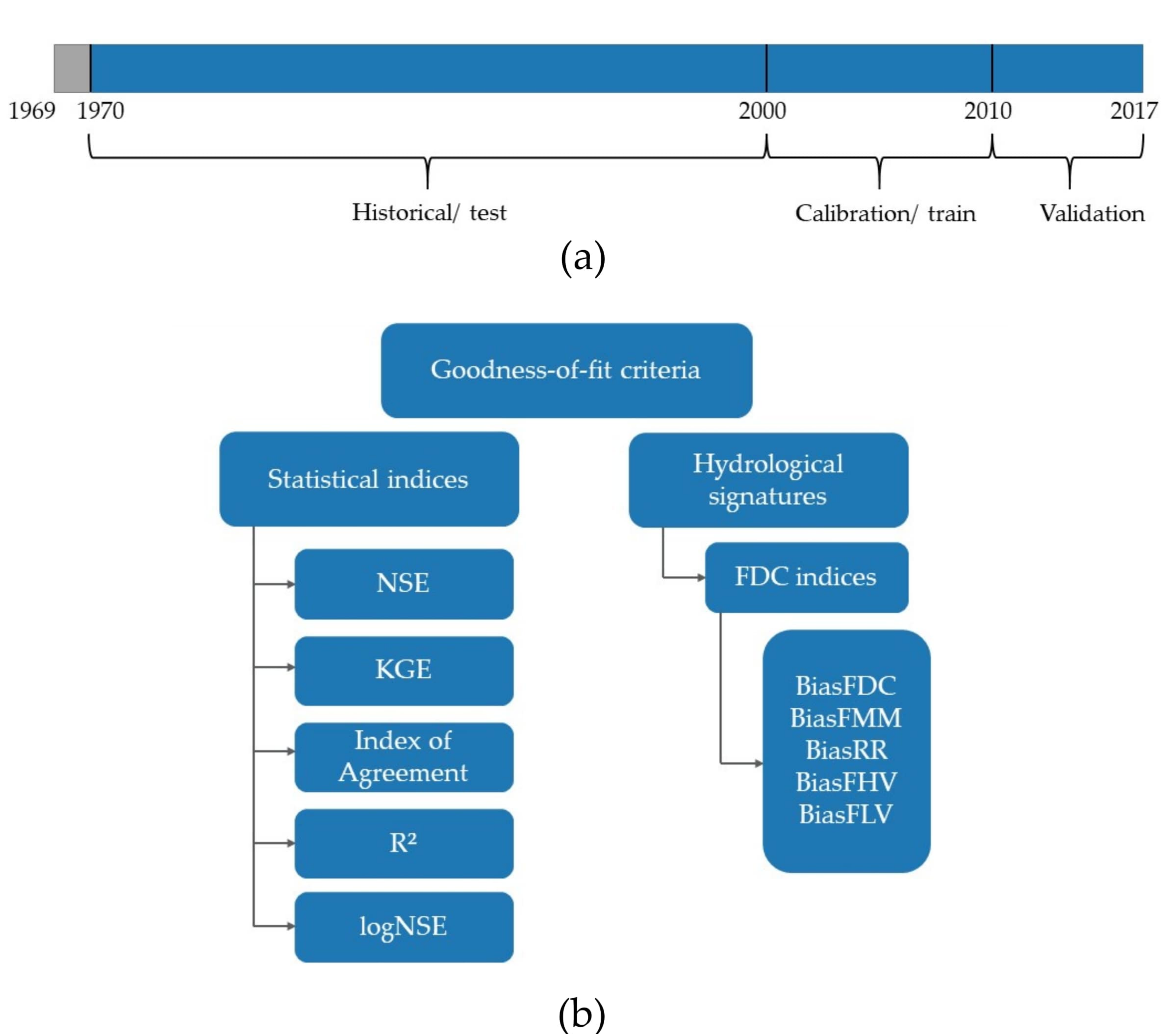
In traditional hydrological modelling, a two-step approach is applied for the calibration and validation procedure, and, therefore, the available time series is divided into two subsets. In ML instead, this process is usually divided in training, validation and test. The training set is used to train the model, and the model performance is evaluated against the validation set. By adjusting the model’s hyperparameters, the best model set-up is found for the validation period. After finishing the hyperparameter tuning the model results are then compared to the test data. In our study, we applied the two-step approach for the HBV model and the three-step approach for the ML models as described in Figure 3a.
To keep up with the sophisticated optimization algorithm for the ML models implemented in PyTorch (Version 1.12.1), a semi-automated calibration process is used for the HBV model. Thus, subjective choice of parameters and impacts of modelers’ decisions are minimized [47]. A wide range between the imaginable maximum and minimum parameter value was simulated for all sensitive input parameters with a relatively small step size in between. The results were compared regarding their Nash–Sutcliffe efficiency (NSE), and the parameter with the best NSE was saved for the final simulations. However, it must be taken into consideration that the internal training algorithm of the ML models minimizes the mean squared error (MSE) of the results.
2.6. Model Evaluation
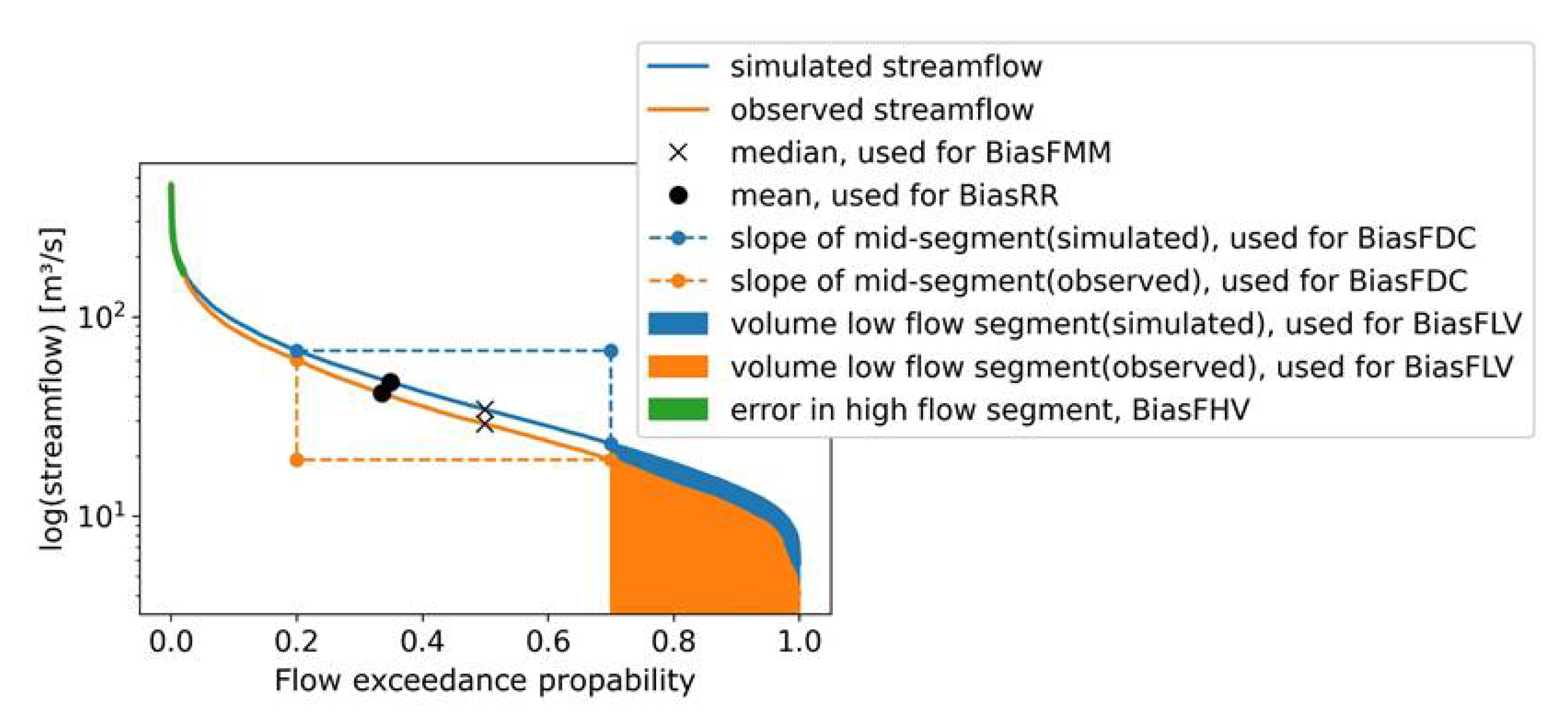
A hydrological model’s performance is usually evaluated using “objective” indices, such as Nash–Sutcliffe efficiency [48], Kling-Gupta efficiency (KGE) [49] and R2. Each metric has its focus, either the overall water balance or a specific flow range [50]. These indices take the whole bandwidth of streamflow into account. Instead, the logNSE uses the logarithmic transformed values of observed and simulated streamflow. This adds more weight on lower values due to its mathematical formulation and, therefore, the logNSE is a recognized low-flow index. However, all these metrics only quantify the statistical characteristics of model residuals, which makes it necessary to include hydrologically based metrics [51]. Examples for hydrologically based metrics are signature indices derived from the flow duration curve [52]. The FDC is the cumulative distribution function where streamflow is plotted against its exceedance probability, showing the percentage of time when streamflow is equal or exceeds the given value [53]. Signature indices examine the influence of specific aspects of the hydrograph and are sensitive to detect differences in runoff generation, seasonality and reactivity [53,54]. Models which show similar NSE values might differ when the FDC is analyzed [54]. We, therefore, used a wide range of various indices, including performance indices and signature indices, to evaluate the model performances and to gain a deep understanding of the models’ strengths and weaknesses (Figure 3b). Due to the widespread application of the performance indices presented in Figure 3b, we refrain from the full explanation of all indices. Here, we explain the five less-common hydrological signature indices we used in this study. They were introduced by [52] in full detail (Figure 4).
- 1.
- Bias RR: bias of the mean values in percent (black circles in Figure 4)
- 2.
- Bias MM: bias of the median values in percent (black crosses Figure 4)
- 3.
- Bias FDC midslope: bias of the mean slope in mid segment of FDC in percent (dashed lines in Figure 4)
- 4.
- Bias FLV: bias of the low segment of the FDC (orange and blue areas in Figure 4)
- 5.
- Bias FHV: bias of the high segment of the FDC (green area in Figure 4)
3. Results
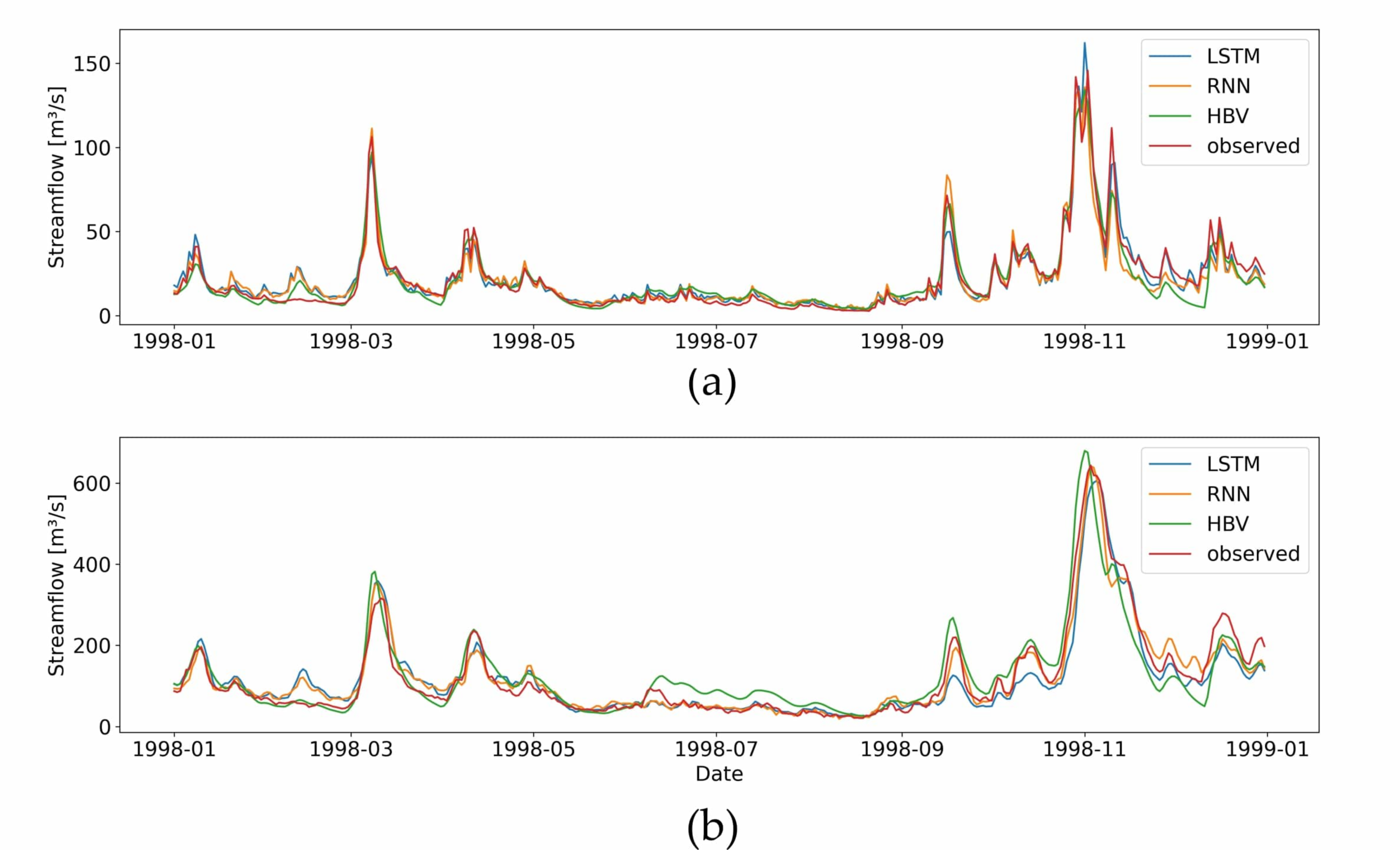
Hydrographs of all models applied in this study are exemplarily displayed in Figure 5 for the most upstream and most downstream located sub-catchments. The hydrographs show the overall good model performance of all models throughout the year but also different response times to streamflow peaks.
3.1. Statistical Performance Indices
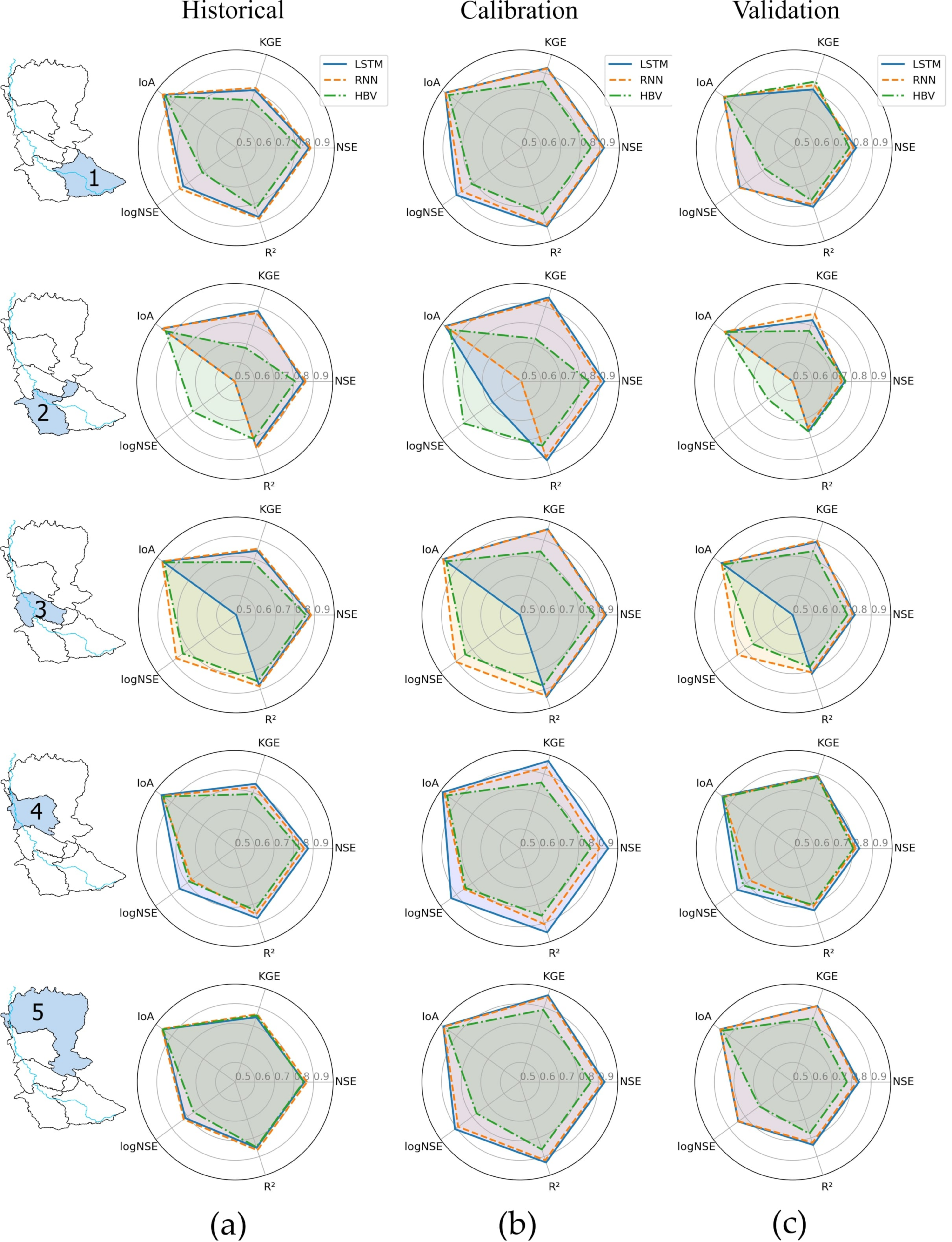
A wide range of performance indices was applied for each sub-catchment and each sub-period (calibration, validation, historical) to evaluate the performance of the different models throughout the catchments (Figure 6).
For the calibration period, the LSTM and RNN perform similarly well for all sub-catchments considering NSE, KGE, R2 and Index of Agreement (IoA), with values of above 0.9, which can be considered “very good” [55]. Focusing on the logNSE, instead, exceptionally lower performance can be observed, particularly in sub-catchments 2 and 3. For the LSTM, the logNSE drops down to 0.68 in sub-catchment 2 and even down to 0.42 in sub-catchment 3, whereas the RNN only shows a decreased logNSE of −1.26 in sub-catchment 2. For the HBV model, the values of NSE, KGE, logNSE, R2 and IoA usually are above 0.8. Exemptions occur in sub-catchment 2 with the KGE ranging slightly above 0.7 and in sub-catchment 5 when the logNSE falls below 0.8.
When looking at the validation and historical period, as expected, all performance indices range lower compared to the calibration. Yet, the overall tendencies described above remain valid: LSTM and RNN perform similarly and usually better than the HBV model for the indices NSE, KGE, R2 and IoA. The differences between the two ML models for each index usually range between 0.05 and 0.1. For the ML models in sub-catchments 1, 3, 4 and 5 during the validation period, the indices NSE, KGE, R2 and IoA are all above 0.8. In sub-catchment 2, those indices only range above 0.7.
The logNSE of RNN and LSTM are between 0.7 and 0.9 within the sub-catchments 1, 4 and 5. In sub-catchments 2 and 3, instead, similar behavior to the calibration can be observed. The LSTM’s logNSE is far below 0.5, whereas the RNN’s logNSE is very low (−1.26) only in sub-catchment 2.
For the HBV model, NSE, KGE, R2 and IoA are all above 0.7 and up to 0.9. Lowest values also tend to occur in sub-catchment 2 and 3. The logNSE generally is also lower than the other indices and is down to 0.66 in sub-catchment 2, but it does not drop as significantly compared to the ML models. During the historical periods, the results are almost similar to the validation period. Larger differences occur only for the HBV model. In sub-catchments 1 and 2, the KGE is about 0.1 lower compared to the validation.
3.2. FDC and Signature Indices
In addition to the traditionally used statistical performance metrics, we analyzed the FDC and signature indices to evaluate the models’ performances for specific flow ranges.
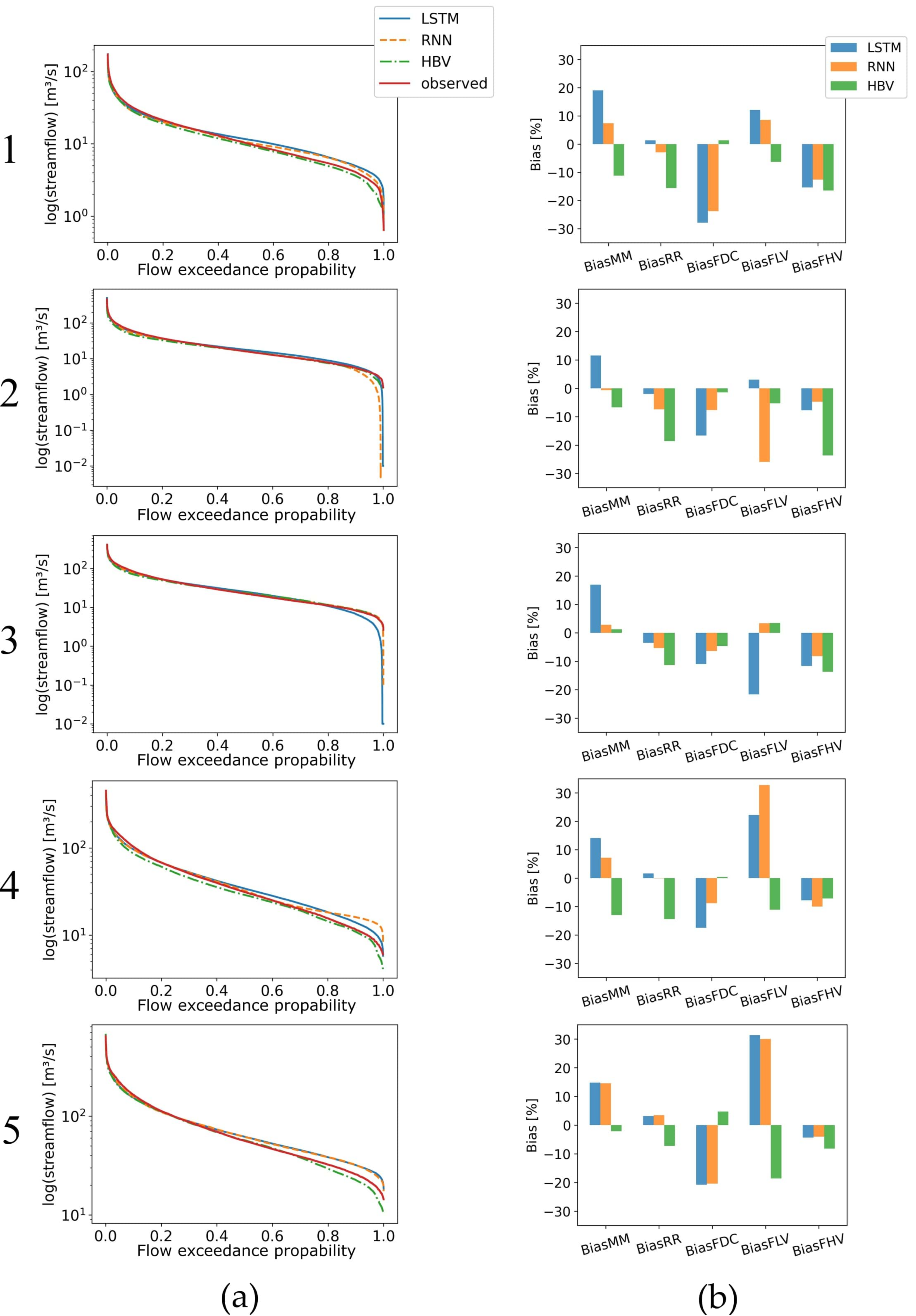
In Figure 7a, the FDCs are shown based on streamflow values of all three sub-periods combined. The bias of the different signature indices is displayed on the right side (Figure 7b). Looking at the FDCs, differences occur mainly in the low-flow section, but this tendency is also exaggerated due to the log-scale applied in Figure 7a.
In the first sub-catchment, the FDCs diverge upwards from 50% flow exceedance probability, with LSTM and RNN tending to overestimate streamflow and the HBV slightly underestimating it. Those observations from the FDC are confirmed by the signature indices. The low-flow bias (BiasFLV) is negative for the HBV and positive for both ML models. Looking at the high-flow bias (BiasFHV) instead, all the models result in a negative bias of around −15% to −20%. The highest biases can be seen for the mid-section slope (BiasFDC). Both ML models have a value below −20%, whereas the HBV’s BiasFDC is only 1.3%. The median bias (BiasMM) is the highest for the LSTM (19.1%) and is −11.2% for the HBV, and for the mean bias (BiasRR), both ML models show a good fit, whereas the HBV has a negative bias of −15.6%.
In sub-catchment 2 and 3, a similar pattern can be observed. The FDCs of the RNN (sub-catchment 2) and the LSTM (sub-catchment 3) show anomalous behavior. In both sub-catchments, the ML models “run dry”, and the FDC decreases far earlier than the observed streamflow. This also leads to a high BiasFLV of below −20% for both models. All other signature index patterns remain comparable to sub-catchment 1, with only the BiasFDC decreasing further downstream for the ML models.
In sub-catchment 4, the FDC of the HBV is located continuously below the observed FDC, which results in negative signature indices throughout the whole set, except for the slope bias. The LSTM’s and RNN’s FDCs exceed the observed values, in particular, in the low-stream section, which results in a large slope bias (BiasFDC) and BiasFLV. In sub-catchment 5, the FDCs show similar behavior to sub-catchment 4. Both ML FDCs are almost equal and show constantly higher streamflow than observed for all values above an exceedance probability of 0.5. This results in a BiasFHV value up to 30% and a BiasFDC of −20%. For the HBV model, signature indices are relatively small. Only the BiasFLV is around −20%.
4. Discussion
In this study we focused on one individual low-land river catchment instead of using a multi-catchment approach for model comparison, which has previously been applied on multiple occasions [40,44] with the capabilities of ML models already highlighted. Five connected sub-catchments were implemented to model streamflow in the Ems catchment and to distinguish potential differences in model performance but also to test whether a simple routing routine works for ML models without the individual model error of each sub-catchment adding up from upstream to downstream. This approach enabled us to analyze the ability of the different models to represent flow dynamics beyond statistical indices.
4.1. Statistical Performance Indices
Looking at the statistical performance indices, in general, the ML models show a superior performance compared to the HBV model within all sub-catchments and almost all indices except the logNSE. Those results are not necessarily surprising, as the ML models are not constrained by the underlying hydrological concept formation of the model developer. ML models develop an individual functional relationship between forcing data and result for every catchment. Instead, conceptual models can struggle with certain catchments and hydrological conditions which do not conform to the assumptions of the developers underlying perceptual model [44]. Yet, the advantages of the hydrological concept formation within conceptual models are visible within the results of sub-catchments 2 and 3. The logNSE values of the LSTM are exceptionally low in sub-catchments 2 and 3 and for the RNN in sub-catchment 2.
Preliminary results of the ML models went below zero for the predicted streamflow within these sub-catchments and had to be manually constrained to a minimum value of 0.01. The lack of physical information in the ML algorithms lead to these weak results in combination with unusual forcing data. In sub-catchment 2 and 3, streamflow from the upstream sub-catchment is used as forcing data, but the differences between outflow and inflow from upstream are relatively low. Sometimes resulting outflow is even smaller than upstream inflow during low-flow periods. Moreover, in other studies, LSTM showed improvement potential for LSTM models during low-flows [56], and Duan et al. [6] found that different ML architectures tend to work better for different flow regimes.
To gain better results for low-flow, it could be beneficial to use a physically informed ML architecture [57] or focus on low-flows in particular during hyperparameter tuning by using the logNSE as the objective function. During ML training, the algorithm minimizes the MSE which focuses on optimizing high-flows due to its mathematical formulation. The parallel use of multiple objective functions can address this issue to some degree by identifying models and hyperparameters that provide sufficient balance between different objectives, such as an accurate representation of different portions of the flow hydrograph [58]. Furthermore, a systematic evaluation and eventual reduction of the input features could further increase the model quality.
4.2. FDC and Signature Indices
The analysis of the FDC allows us to distinguish systematic differences between the model results and particular streamflow ranges. Each model’s FDC does show a unique shape compared to other sub-catchments. This can be expected as we trained the models individually. In sub-catchment 2 and 3, the curve for the ML models drops too early compared to the observed streamflow. This indicates that the models do not simulate the correct retention of precipitation or internal storage. Furthermore, the RNN model shows a contrary behavior in sub-catchment 4, and the FDC reveals that the model systematically overestimates streamflow. The signature indices now help to sample the model performance for specific parts of the FDC. Some signature indices show a continuous signal for each model and sub-catchment, whereas other signature indices are highly variable. In general, the ML models show a low BiasRR and sufficiently manage to simulate the observed water balance. Whereas the HBV continuously has a low BiasFDC within all sub-catchments. This indicates that the HBV model has its strength in modelling the right streamflow dynamics after precipitation events. The ML models, instead, show a negative BiasFDC indicating a slower reaction of streamflow compared to the observed values.
The topic of low-flows was already discussed in Section 4.1 while focusing on the statistical indices. The low-flow bias (BiasFLV) is highly variable for all models and sub-catchments. The visible drop of the ML models in sub-catchment 2 and 3, respectively, results in the expected underestimation of streamflow. Moreover, in sub-catchments 4 and 5, where logNSE values are fairly good, above 0.7, the BiasFLV is high, up to +30%. This underlines the previously mentioned possibility for improvements in the low-flow section by Gauch et al. [56]. Regarding the high-flow bias (BiasFHV), all models within all sub-catchments show an underestimation of streamflow peaks. Yet, hydrological models as well as ML models tend to underpredict high streamflow [40,44]. This is due to the non-linear dynamics of threshold behavior within a catchment.
4.3. RNN Compared to LSTM
In traditional RNN structures, a maximum of ten timesteps is remembered by the model [39], and Kratzert et al. [40] argue that RNNs, therefore, are not capable to model catchments with long-term storage processes longer than this period. Yet, baseflow is the dominating streamflow generation process in the Ems catchment [27], and baseflow response to precipitation in Germany tends to be at least one month [59]. Following the idea that RNN cannot model storage effects longer than ten days, the results of the RNN model should be insufficient. However, our results showed a good streamflow prediction in four of five sub-catchments. This is comparable to the LSTM models, which are capable of incorporating long-term dependencies.
On the other hand, the low-flow index logNSE showed a decreased model performance in sub-catchment 2, which is the expectable behavior as, during low-flow periods, the importance of correct baseflow modelling is even higher [40]. A possible explanation is that input features could indirectly contain the missing information or have a strong correlation to the drivers of long-term dependencies in the catchment. In particular, this could be the case in sub-catchments 2–5 when modelled streamflow is used as an input feature. Further investigations on baseflow characteristics in the catchment and corresponding processes within the RNN would be necessary to overcome this discrepancy.
4.4. Routing
We applied a simple routing routine in the ML models and used simulated streamflow from the upstream sub-catchment as forcing data for model predictions. Every model is a simplification of reality. This induces structural uncertainty. As modelled results were used as input for the downstream model, it was questionable on how the model adapts to that inaccurate information.
Going from upstream to downstream, no continuous decrease of statistical indices can be observed. Instead, in sub-catchment 5, the statistical indices overall show the best performance within all sub-catchments. The performance is even better than in sub-catchment 1, which technically is a single-basin approach. Therefore, a significant improvement in model results would not be expected compared to a methodology that applies a single model for the entire basin.
Each ML model shows an individual shape of the FDC on the first sight. Growing distances between observed and modelled streamflow are not visible. The analysis of the signature indices is more accurate. Not a single signature index rises continuously over all sub-catchments, so model biases appear not to accumulate. Accordingly, the ML models can mitigate the effect of uncertainty-containing input information. However, it remains unsure how this uncertainty exactly influences the results. It could be possible that the extremely low logNSE values and large BiasFLV values result from insufficient upstream inflow information. Yet, it could be further investigated how the ML uses the inaccurate input information using eXplainable Artificial Intelligence (XAI) techniques or by testing the models with systematically biased data.
5. Conclusions
This study presents a model intercomparison between two ML models, RNN and LSTM, and the conceptual hydrological model HBV for a low-land river catchment. Similar to other studies, the ML models showed a superior model performance compared to the HBV for a wide range of indices (NSE, KGE, R2 and IoA). Signature indices, sampling specific parts of the FDC, reveal that the ML models have good representation of the overall water balance (low BiasRR), whereas the HBV model provides a better representation of streamflow dynamics (low BiasFDC). Further research is necessary to determine if this is a general model behavior or if this phenomenon only applies to catchments with certain characteristics.
Yet, both ML show decreased performance for the logNSE in one (RNN) and two (LSTM) sub-catchments. For future applications regarding low-flows, the performance of the ML models should be specifically evaluated using an appropriate low-flow index. In particular, when the MSE was used as the objective function during model training, which does not show sensitivity to low streamflow due to its quadratic character.
The models were tested in a catchment with a major baseflow share of total streamflow, and baseflow can be considered the long-term component of streamflow. Yet, RNNs are known to only memorize the previous ten timesteps, in our case ten days, for the modelling process. The RNN models obtained good results in four of five sub-catchments, however. Why the RNN models are actually capable of correctly representing the streamflow with the expectable long-term dependencies in the study area remains unsure. On the other hand, the network architecture of the LSTM should be able to represent baseflow dynamics accordingly, but both models show weaknesses in the correct representation of low-flows, when baseflow has its greatest relevance in streamflow generation. Linking the catchments storage effects to the LSTM internal states and the use of explainable artificial intelligence methods could help to disclose whether an incorrect representation of baseflow or only the use of the MSE objective function explain the low-flow results.
Regarding the routing routine tested in this study, the qualitative evaluation of statistical indices and signature indices revealed no growing biases upstream-to-downstream. However, further in-depth analysis including qualitative approaches has to be carried out to gain an understanding of the type and behavior of the potential errors and uncertainties.
Author Contributions
Conceptualization, A.L., H.B. and M.C.; writing—original draft preparation, A.L.; writing—review and editing, A.L., H.B. and M.C.; funding acquisition, H.B. All authors have read and agreed to the published version of the manuscript.
Funding
This research was funded by the German Federal Ministry of Education and Research (BMBF) (grant number: 01LR2003A) within the project WAKOS—Wasser an den Küsten Ostfrieslands.
Data Availability Statement
The data presented in this study are available upon request from the corresponding author.
Conflicts of Interest
The authors declare no conflict of interest.
References
- Bergström, S.; Forsman, A. Development of a Conceptual Deterministic Rainfall-Runoff Model. Hydrol. Res. 1973, 4, 147–170. [Google Scholar] [CrossRef]
- Bergström, S. The HBV Model: Its Structure and Applications. SMHI Rep. Hydrol. 1992, 4, 35. [Google Scholar]
- Beven, K.; Binley, A. The Future of Distributed Models: Model Calibration and Uncertainty Prediction. Hydrol. Process. 1992, 6, 279–298. [Google Scholar] [CrossRef]
- Refsgaard, J.C.; Storm, B. Construction, Calibration and Validation of Hydrological Models. In Distributed Hydrological Modelling; Abbott, M.B., Refsgaard, J.C., Eds.; Water Science and Technology Library; Springer: Dordrecht, The Netherlands, 1996; pp. 41–54. ISBN 978-94-009-0257-2. [Google Scholar]
- Liu, Z.; Zhou, P.; Zhang, Y. A Probabilistic Wavelet–Support Vector Regression Model for Streamflow Forecasting with Rainfall and Climate Information Input. J. Hydrometeorol. 2015, 16, 2209–2229. [Google Scholar] [CrossRef]
- Duan, S.; Ullrich, P.; Shu, L. Using Convolutional Neural Networks for Streamflow Projection in California. Front. Water 2020, 2, 28. [Google Scholar] [CrossRef]
- Schmidt, L.; Heße, F.; Attinger, S.; Kumar, R. Challenges in Applying Machine Learning Models for Hydrological Inference: A Case Study for Flooding Events Across Germany. Water Resour. Res. 2020, 56, e2019WR025924. [Google Scholar] [CrossRef]
- Gao, C.; Gemmer, M.; Zeng, X.; Liu, B.; Su, B.; Wen, Y. Projected Streamflow in the Huaihe River Basin (2010–2100) Using Artificial Neural Network. Stoch Env. Res Risk Assess 2010, 24, 685–697. [Google Scholar] [CrossRef]
- Noori, N.; Kalin, L. Coupling SWAT and ANN Models for Enhanced Daily Streamflow Prediction. J. Hydrol. 2016, 533, 141–151. [Google Scholar] [CrossRef]
- Peng, T.; Zhou, J.; Zhang, C.; Fu, W. Streamflow Forecasting Using Empirical Wavelet Transform and Artificial Neural Networks. Water 2017, 9, 406. [Google Scholar] [CrossRef] [Green Version]
- Kisi, O.; Cimen, M. A Wavelet-Support Vector Machine Conjunction Model for Monthly Streamflow Forecasting. J. Hydrol. 2011, 399, 132–140. [Google Scholar] [CrossRef]
- Huang, S.; Chang, J.; Huang, Q.; Chen, Y. Monthly Streamflow Prediction Using Modified EMD-Based Support Vector Machine. J. Hydrol. 2014, 511, 764–775. [Google Scholar] [CrossRef]
- Kratzert, F.; Klotz, D.; Shalev, G.; Klambauer, G.; Hochreiter, S.; Nearing, G. Towards Learning Universal, Regional, and Local Hydrological Behaviors via Machine Learning Applied to Large-Sample Datasets. Hydrol. Earth Syst. Sci. 2019, 23, 5089–5110. [Google Scholar] [CrossRef] [Green Version]
- Le; Ho; Lee; Jung Application of Long Short-Term Memory (LSTM) Neural Network for Flood Forecasting. Water 2019, 11, 1387. [CrossRef] [Green Version]
- Feng, D.; Fang, K.; Shen, C. Enhancing Streamflow Forecast and Extracting Insights Using Long-Short Term Memory Networks With Data Integration at Continental Scales. Water Resour. Res. 2020, 56, e2019WR026793. [Google Scholar] [CrossRef]
- Scorzini, A.R.; Di Bacco, M.; De Luca, G.; Tallini, M. Deep Learning for Earthquake Hydrology? Insights from the Karst Gran Sasso Aquifer in Central Italy. J. Hydrol. 2023, 617, 129002. [Google Scholar] [CrossRef]
- Zhou, R.; Zhang, Y. On the Role of the Architecture for Spring Discharge Prediction with Deep Learning Approaches. Hydrol. Process. 2022, 36, e14737. [Google Scholar] [CrossRef]
- Chang, Y.-S.; Chiao, H.-T.; Abimannan, S.; Huang, Y.-P.; Tsai, Y.-T.; Lin, K.-M. An LSTM-Based Aggregated Model for Air Pollution Forecasting. Atmos. Pollut. Res. 2020, 11, 1451–1463. [Google Scholar] [CrossRef]
- Haq, M.; Jilani, A.; Prabu, P. Deep Learning Based Modeling of Groundwater Storage Change. CMC 2021, 70, 4599–4617. [Google Scholar] [CrossRef]
- Le, X.-H.; Nguyen, D.-H.; Jung, S.; Yeon, M.; Lee, G. Comparison of Deep Learning Techniques for River Streamflow Forecasting. IEEE Access 2021, 9, 71805–71820. [Google Scholar] [CrossRef]
- Solgi, R.; Loáiciga, H.A.; Kram, M. Long Short-Term Memory Neural Network (LSTM-NN) for Aquifer Level Time Series Forecasting Using in-Situ Piezometric Observations. J. Hydrol. 2021, 601, 126800. [Google Scholar] [CrossRef]
- Anul Haq, M. CDLSTM: A Novel Model for Climate Change Forecasting. Comput. Mater. Contin. 2022, 71, 2363–2381. [Google Scholar] [CrossRef]
- Seibert, J.; Bergström, S. A Retrospective on Hydrological Catchment Modelling Based on Half a Century with the HBV Model. Hydrol. Earth Syst. Sci. 2022, 26, 1371–1388. [Google Scholar] [CrossRef]
- Loganathan, P.; Mahindrakar, A.B. Intercomparing the Robustness of Machine Learning Models in Simulation and Forecasting of Streamflow. J. Water Clim. Change 2020, 12, 1824–1837. [Google Scholar] [CrossRef]
- Wheater, H.S.; Peach, D.; Binley, A. Characterising Groundwater-Dominated Lowland Catchments: The UK Lowland Catchment Research Programme (LOCAR). Hydrol. Earth Syst. Sci. 2007, 11, 108–124. [Google Scholar] [CrossRef]
- Geschäftsstelle Ems; Ministerie van Verkeer en Waterstaa; Geschäftsstelle Ems-NRW. Internationaler Bewirtschaftungplan nach Artikel 13 Wasserrahmenrichtlinie für die Flussgebietseinheit Ems; Geschäftsstelle der FGG Ems: Meppen, Germany, 2009. [Google Scholar]
- Wendland, F.; Bogena, H.; Goemann, H.; Hake, J.F.; Kreins, P.; Kunkel, R. Impact of Nitrogen Reduction Measures on the Nitrogen Loads of the River Ems and Rhine (Germany). Phys. Chem. Earth Parts A/B/C 2005, 30, 527–541. [Google Scholar] [CrossRef]
- DWD Climate Data Center. Available online: https://www.dwd.de/EN/climate_environment/cdc/cdc_node_en.html (accessed on 30 November 2022).
- BFG Global Runoff Data Centre. Available online: https://www.bafg.de/GRDC/EN/Home/homepage_node.html (accessed on 30 November 2022).
- European Environment Agency; European Union; Copernicus Land Monitoring Service. Corine Land Cover; European Environment Agency: Copenhagen, Denmark, 2018. [Google Scholar]
- Haude, W. Zur Bestimmung Der Verdunstung Auf Möglichst Einfache Weise. Mitt Dt Wetterd 1955, 11, 1–24. [Google Scholar]
- Götzinger, J.; Bárdossy, A. Comparison of Four Regionalisation Methods for a Distributed Hydrological Model. J. Hydrol. 2006, 333, 374–384. [Google Scholar] [CrossRef]
- Wrede, S.; Seibert, J.; Uhlenbrook, S. Distributed Conceptual Modelling in a Swedish Lowland Catchment: A Multi-Criteria Model Assessment. Hydrol. Res. 2013, 44, 318–333. [Google Scholar] [CrossRef] [Green Version]
- Booij, M.J.; Krol, M.S. Balance between Calibration Objectives in a Conceptual Hydrological Model. Hydrol. Sci. J. 2010, 55, 1017–1032. [Google Scholar] [CrossRef]
- Výleta, R.; Sleziak, P.; Hlavčová, K.; Danáčová, M.; Aleksić, M.; Szolgay, J.; Kohnová, S. An HBV-Model Based Approach for Studying the Effects of Projected Climate Change on Water Resources in Slovakia; Copernicus Meetings: Vienna, Austria, 2022. [Google Scholar]
- Breuer, L.; Huisman, J.A.; Willems, P.; Bormann, H.; Bronstert, A.; Croke, B.F.W.; Frede, H.-G.; Gräff, T.; Hubrechts, L.; Jakeman, A.J.; et al. Assessing the Impact of Land Use Change on Hydrology by Ensemble Modeling (LUCHEM). I: Model Intercomparison with Current Land Use. Adv. Water Resour. 2009, 32, 129–146. [Google Scholar] [CrossRef]
- Devia, G.K.; Ganasri, B.P.; Dwarakish, G.S. A Review on Hydrological Models. Aquat. Procedia 2015, 4, 1001–1007. [Google Scholar] [CrossRef]
- Werbos, P.J. Generalization of Backpropagation with Application to a Recurrent Gas Market Model. Neural Netw. 1988, 1, 339–356. [Google Scholar] [CrossRef]
- Bengio, Y.; Simard, P.; Frasconi, P. Learning Long-Term Dependencies with Gradient Descent Is Difficult. IEEE Trans. Neural Netw. 1994, 5, 157–166. [Google Scholar] [CrossRef]
- Kratzert, F.; Klotz, D.; Brenner, C.; Schulz, K.; Herrnegger, M. Rainfall–Runoff Modelling Using Long Short-Term Memory (LSTM) Networks. Hydrol. Earth Syst. Sci. 2018, 22, 6005–6022. [Google Scholar] [CrossRef] [Green Version]
- Hochreiter, S.; Schmidhuber, J. Long Short-Term Memory. Neural Comput. 1997, 9, 1735–1780. [Google Scholar] [CrossRef]
- Li, P.; Zhang, J.; Krebs, P. Prediction of Flow Based on a CNN-LSTM Combined Deep Learning Approach. Water 2022, 14, 993. [Google Scholar] [CrossRef]
- Kratzert, F.; Klotz, D.; Gauch, M.; Klingler, C.; Nearing, G.; Hochreiter, S. Large-Scale River Network Modeling Using Graph Neural Networks. In Proceedings of the 23rd EGU General Assembly, Virtual, 19–30 April 2021. [Google Scholar]
- Lees, T.; Buechel, M.; Anderson, B.; Slater, L.; Reece, S.; Coxon, G.; Dadson, S.J. Benchmarking Data-Driven Rainfall–Runoff Models in Great Britain: A Comparison of Long Short-Term Memory (LSTM)-Based Models with Four Lumped Conceptual Models. Hydrol. Earth Syst. Sci. 2021, 25, 5517–5534. [Google Scholar] [CrossRef]
- Althoff, D.; Rodrigues, L.N.; Silva, D.D. da Addressing Hydrological Modeling in Watersheds under Land Cover Change with Deep Learning. Adv. Water Resour. 2021, 154, 103965. [Google Scholar] [CrossRef]
- Haq, M.A.; Ahmed, A.; Khan, I.; Gyani, J.; Mohamed, A.; Attia, E.-A.; Mangan, P.; Pandi, D. Analysis of Environmental Factors Using AI and ML Methods. Sci Rep 2022, 12, 13267. [Google Scholar] [CrossRef]
- Bormann, H.; De Brito, M.M.; Charchousi, D.; Chatzistratis, D.; David, A.; Grosser, P.F.; Kebschull, J.; Konis, A.; Koutalakis, P.; Korali, A.; et al. Impact of Hydrological Modellers’ Decisions and Attitude on the Performance of a Calibrated Conceptual Catchment Model: Results from a ‘Modelling Contest. Hydrology 2018, 5, 64. [Google Scholar] [CrossRef] [Green Version]
- Nash, J.E.; Sutcliffe, J.V. River Flow Forecasting through Conceptual Models Part I—A Discussion of Principles. J. Hydrol. 1970, 10, 282–290. [Google Scholar] [CrossRef]
- Gupta, H.V.; Kling, H.; Yilmaz, K.K.; Martinez, G.F. Decomposition of the Mean Squared Error and NSE Performance Criteria: Implications for Improving Hydrological Modelling. J. Hydrol. 2009, 377, 80–91. [Google Scholar] [CrossRef]
- Bai, P.; Liu, X.; Xie, J. Simulating Runoff under Changing Climatic Conditions: A Comparison of the Long Short-Term Memory Network with Two Conceptual Hydrologic Models. J. Hydrol. 2021, 592, 125779. [Google Scholar] [CrossRef]
- Van Werkhoven, K.; Wagener, T.; Reed, P.; Tang, Y. Sensitivity-Guided Reduction of Parametric Dimensionality for Multi-Objective Calibration of Watershed Models. Adv. Water Resour. 2009, 32, 1154–1169. [Google Scholar] [CrossRef]
- Yilmaz, K.K.; Gupta, H.V.; Wagener, T. A Process-Based Diagnostic Approach to Model Evaluation: Application to the NWS Distributed Hydrologic Model. Water Resour. Res. 2008, 44, 1–18. [Google Scholar] [CrossRef] [Green Version]
- Casper, M.C.; Grigoryan, G.; Gronz, O.; Gutjahr, O.; Heinemann, G.; Ley, R.; Rock, A. Analysis of Projected Hydrological Behavior of Catchments Based on Signature Indices. Hydrol. Earth Syst. Sci. 2012, 16, 409–421. [Google Scholar] [CrossRef] [Green Version]
- Ley, R.; Hellebrand, H.; Casper, M.C.; Fenicia, F. Comparing Classical Performance Measures with Signature Indices Derived from Flow Duration Curves to Assess Model Structures as Tools for Catchment Classification. Hydrol. Res. 2016, 47, 1–14. [Google Scholar] [CrossRef] [Green Version]
- Moriasi, D.N.; Arnold, J.G.; Liew, M.W.V.; Bingner, R.L.; Harmel, R.D.; Veith, T.L. Model Evaluation Guidelines for Systematic Quantification of Accuracy in Watershed Simulations. Trans. ASABE 2007, 50, 885–900. [Google Scholar] [CrossRef]
- Gauch, M.; Kratzert, F.; Klotz, D.; Nearing, G.; Lin, J.; Hochreiter, S. Rainfall–Runoff Prediction at Multiple Timescales with a Single Long Short-Term Memory Network. Hydrol. Earth Syst. Sci. 2021, 25, 2045–2062. [Google Scholar] [CrossRef]
- Zhang, L.; Bellugi, D.; Kadi, J.; Kamat, A.; Gorski, G.; Larsen, L. Physics-Informed LSTM for Streamflow Modeling Using a Dataset of Intensively-Monitored Watersheds in the USA. In Proceedings of the AGU Fall Meeting 2021, New Orleans, LA, USA, 13–17 December 2021. [Google Scholar]
- De Vos, N.J.; Rientjes, T.H.M. Multiobjective Training of Artificial Neural Networks for Rainfall-Runoff Modeling. Water Resour. Res. 2008, 44, W08434. [Google Scholar] [CrossRef] [Green Version]
- Hellwig, J.; Stahl, K. An Assessment of Trends and Potential Future Changes in Groundwater-Baseflow Drought Based on Catchment Response Times. Hydrol. Earth Syst. Sci. 2018, 22, 6209–6224. [Google Scholar] [CrossRef]
Figure 1.
(a) Overview map of the study area location in Germany. (b,c) Maps of the river Ems showing the five individual sub-catchments delineated upstream from the last available streamflow gauge located 235 km downstream from the spring with its streamflow gauges, land use (b) and elevation (c). It appears that six separated catchments were delineated; yet, the smallest one actually has a connection to sub-catchment 2 on the bottom left side.

Figure 2.
(a) The architecture of a RNN cell is displayed on the left side with x being the input and h the internal state; t indicates the current timestep. (b) Internals of the LSTM cell with h referring to the hidden state, c the cell state, f the forget gate, i the input gate and o the output gate at timestep t. Further details are explained by Equations (3)–(8).

Figure 3.
(a) Time ranges applied for the different model types during the modeling process. (b) Overview of all goodness-of-fit criteria used to evaluate the model results.
Figure 3.
(a) Time ranges applied for the different model types during the modeling process. (b) Overview of all goodness-of-fit criteria used to evaluate the model results.

Figure 4.
Two exemplary flow duration curves with highlighted features to explain the signature indices after Casper et al. [53].
Figure 4.
Two exemplary flow duration curves with highlighted features to explain the signature indices after Casper et al. [53].

Figure 5.
Hydrographs of all models and observed streamflow within sub-catchment 1 (a) and sub-catchment 5 (b) in the year 1998 to show annual variations in streamflow and the models’ performances exemplarily.
Figure 5.
Hydrographs of all models and observed streamflow within sub-catchment 1 (a) and sub-catchment 5 (b) in the year 1998 to show annual variations in streamflow and the models’ performances exemplarily.

Figure 6.
Radar plots showing the variety of statistical indices for the five different sub-catchments and the three different periods (historical (a), calibration (b) and validation (c)). The minimal value visible in this figure is 0.5. Yet, in catchment 2 and 3, the logNSE value can be lower than 0.5, and, therefore, the logNSE values below 0.5 are mentioned in the following. Sub-catchment 2 (historical: LSTM: 0.45, RNN: −1.71; calibration: RNN: −1.26; validation: LSTM: 0.23, RNN: −1.80); Sub-catchment 3 (historical: LSTM: −0.47; calibration: LSTM: 0.42; validation: −0.11).

Figure 7.
(a) Flow duration curves of all three model types and observed streamflow. (b) Bias of the five signature indices for the three model types compared to the observed streamflow.
Figure 7.
(a) Flow duration curves of all three model types and observed streamflow. (b) Bias of the five signature indices for the three model types compared to the observed streamflow.


Table 1.
Number and data source of hydro–climatic stations used to derive forcing data for the models and to calculate the potential evapotranspiration.
Table 1.
Number and data source of hydro–climatic stations used to derive forcing data for the models and to calculate the potential evapotranspiration.
| Data | Number of Stations | Source | Required For |
|---|---|---|---|
| Precipitation (daily sum) | 142 | DWD | HBV, LSTM, RNN |
| Rel. Humidity (hourly mean) | 10 | DWD | HBV (pET estimation after Haude [31]) |
| Maximum Temperature (daily) | 25 | DWD | LSTM, RNN |
| Minimum Temperature (daily) | 25 | DWD | LSTM, RNN |
| Temperature (daily mean) | 33 | DWD | HBV |
| Temperature (hourly mean) | 8 | DWD | HBV (pET estimation after Haude [31]) |
| Vapor Pressure (daily mean) | 29 | DWD | LSTM, RNN |
| Streamflow (daily mean) | 5 | GRDC | HBV, LSTM, RNN |
Table 2.
Area (m2), flow length (km) and baseflow index (BFI) (baseflow/total streamflow) for each of the five individual sub-catchments. Sub-catchments are numbered systematically upstream-to-downstream.
Table 2.
Area (m2), flow length (km) and baseflow index (BFI) (baseflow/total streamflow) for each of the five individual sub-catchments. Sub-catchments are numbered systematically upstream-to-downstream.
| Number of Sub-catchment | Area (km2) | Flow Length (km) | BFI (%) |
|---|---|---|---|
| 1 | 1448 | 87 | 55 |
| 2 | 1283 | 26 | 51 |
| 3 | 871 | 40 | 57 |
| 4 | 1150 | 59 | 61 |
| 5 | 3324 | 22 | 55 |
Disclaimer/Publisher’s Note: The statements, opinions and data contained in all publications are solely those of the individual author(s) and contributor(s) and not of MDPI and/or the editor(s). MDPI and/or the editor(s) disclaim responsibility for any injury to people or property resulting from any ideas, methods, instructions or products referred to in the content. |
© 2023 by the authors. Licensee MDPI, Basel, Switzerland. This article is an open access article distributed under the terms and conditions of the Creative Commons Attribution (CC BY) license (https://creativecommons.org/licenses/by/4.0/).
Share and Cite
MDPI and ACS Style
Ley, A.; Bormann, H.; Casper, M. Intercomparing LSTM and RNN to a Conceptual Hydrological Model for a Low-Land River with a Focus on the Flow Duration Curve. Water 2023, 15, 505. https://doi.org/10.3390/w15030505
AMA Style
Ley A, Bormann H, Casper M. Intercomparing LSTM and RNN to a Conceptual Hydrological Model for a Low-Land River with a Focus on the Flow Duration Curve. Water. 2023; 15(3):505. https://doi.org/10.3390/w15030505
Chicago/Turabian StyleLey, Alexander, Helge Bormann, and Markus Casper. 2023. "Intercomparing LSTM and RNN to a Conceptual Hydrological Model for a Low-Land River with a Focus on the Flow Duration Curve" Water 15, no. 3: 505. https://doi.org/10.3390/w15030505
Note that from the first issue of 2016, this journal uses article numbers instead of page numbers. See further details here.