Research on Parameter Regionalization of Distributed Hydrological Model Based on Machine Learning

Abstract

In the past decade, more than 300 people have died per year on average due to mountain torrents in China. Mountain torrents mostly occur in ungauged small and medium-sized catchments, so it is difficult to maintain high accuracy of flood prediction. In order to solve the problem of the low accuracy of flood simulation in the ungauged areas, this paper studies the influence of different methods on the parameter regionalization of distributed hydrological model parameters in hilly areas of Hunan Province. According to the terrain, landform, soil and land use characteristics of each catchment, we use Shortest Distance, Attribute Similarity, Support Vector Regression, Generative Adversarial Networks, Classification and Regression Tree and Random Forest methods to create parameter regionalization schemes. In total, 426 floods of 25 catchments are selected to calibrate the model parameters, and 136 floods of 8 catchments are used for verification. The results showed that the average values of the Nash–Sutcliffe coefficients of each scheme were 0.58, 0.64, 0.60, 0.66, 0.61 and 0.68, and the worst values were 0.27, 0.31, 0.25, 0.43, 0.35 and 0.59. The random forest model is the most stable solution and significantly outperforms other methods. Using the random forest model to regionalize parameters can improve the accuracy of flood simulation in ungauged areas, which is of great significance for flash flood forecasting and early warning.

1. Introduction

Hunan Province is located in the southeast inland of China, with abundant rainfall but extremely uneven temporal and spatial distribution. Due to frequent and high-intensity rainfall and short confluence time in hilly areas, the flood rises and falls steeply, which can very easily cause mountain torrents. The climate, underlying surface and geomorphic types in hilly areas are diverse, and most of them are areas without data. This is an important challenge for flood forecasting and early warning in hilly areas.

The hydrological model is an important tool for understanding the laws of hydrological science, analyzing hydrological processes and studying hydrological cycle mechanisms [1]. How to identify hydrological parameters in ungauged areas accurately is an important area of research for PUB (Prediction in Ungauged Basins). The regionalization method is usually used to determine the parameters of hydrological models for ungauged basins at present, and the commonly used methods include shortest distance, attribute similarity, regression, average, machine learning, etc. The main idea of the regionalization method is to analyze the relationship between model parameters and characteristic attributes of basins, and the parameters of the hydrological model for ungauged basins are deduced from the calibration results of gauged basins [2].

The parameter transplant method includes the shortest distance method and the attribute similarity method. Among them, the distance approach refers to finding one or more basins adjacent to the research object in the geographical location. The attribute similarity method is used to find a basin that is similar to the research basin in attributes. Young achieved the ideal result of parameter transplant by computing the spatial distance between 260 catchments in the UK [3]. Parajka et al. selected indicators such as watershed area, average slope, watershed latitude, river network density, vegetation coverage, drought index, etc., to analyze the similarity of watershed attributes and complete parameter transplantation. The results show that attribute selection plays a decisive role in the performance of transplantation [4]. Li et al. compared the shortest distance method with the attribute similarity method and pointed out that the performance of transplantation results is affected by the density of hydrological stations, and it is easier to achieve better results in areas with dense hydrological stations [5].

The parameter regression method is mainly used to establish the functional relationship between watershed characteristics and model parameters. Yokoo et al. established a multiple linear regression equation between the Tank model parameters and soil, geology and land use data [6]. Cheng et al. established a regression equation between the SCS model parameter CN, concentration time and soil, land use, average slope and river length [7]. Based on the parameter regionalization method combining spatial proximity and stepwise regression analysis, Yao et al. found that stepwise regression analysis can effectively deduce the sensitive parameters [8]. Sun et al. pointed out that the parametric regression method is prone to the phenomenon of “the same effect of different parameters”, and the basin properties screening is highly subjective, which is not suitable for small samples [9].

Machine learning research mainly includes SOM classification and the CART decision tree method. Yi et al. used hierarchical clustering analysis HCA and unsupervised neural network SOM methods to divide the sub basins of Dianchi Lake basin into 7 groups based on 16 physical characteristics, and they believed that the basin parameters of the same group can be transplanted to each other [10]. Ragettli et al. took 35 basins in different regions of China as the research object, comprehensively considering the physical properties of watersheds and the spatial distance of watersheds; the CART tree model was used to optimize the parameter transplantation rules, and the results show that the CART tree has better parameter adaptability [11]. Liu et al. conducted a parametric zoning study on 19 small catchments in Henan Province; the success rate of parameter transplantation based on the CART tree is about 20% higher than that of random transplantation [12].

The advantage of the CART tree is that it is easy to interpret and the mapping between basin characteristics and transplantation rules is intuitive. In recent years, with the advent of machine learning algorithms, more and more models have been used to create parameter transplantation schemes. However, many machine learning algorithms usually require a large number of samples, and data showing that hydrological model modeling can be used for parameter calibration is often very limited, so it is necessary to reasonably build a large number of learning samples, or to study intelligent algorithms suitable for small sample research. In this study, 33 small and medium-sized catchments in Hunan Province were taken as examples. We constructed distributed hydrological models of these catchments and selected four machine learning models—Support Vector Regression, Generative Adversarial Networks, Classification and Regression Tree, and Random Forest—to create different parametric regionalization schemes and compared them with two traditional methods—Shortest Distance and Attribute Similarity. By analyzing the transplantation results of different schemes, it can provide a reference for determining the parameters of the distributed hydrological model in ungauged areas, which is very valuable for flash flood forecasting and early warning.

2. Materials and Methods

2.1. Study Area

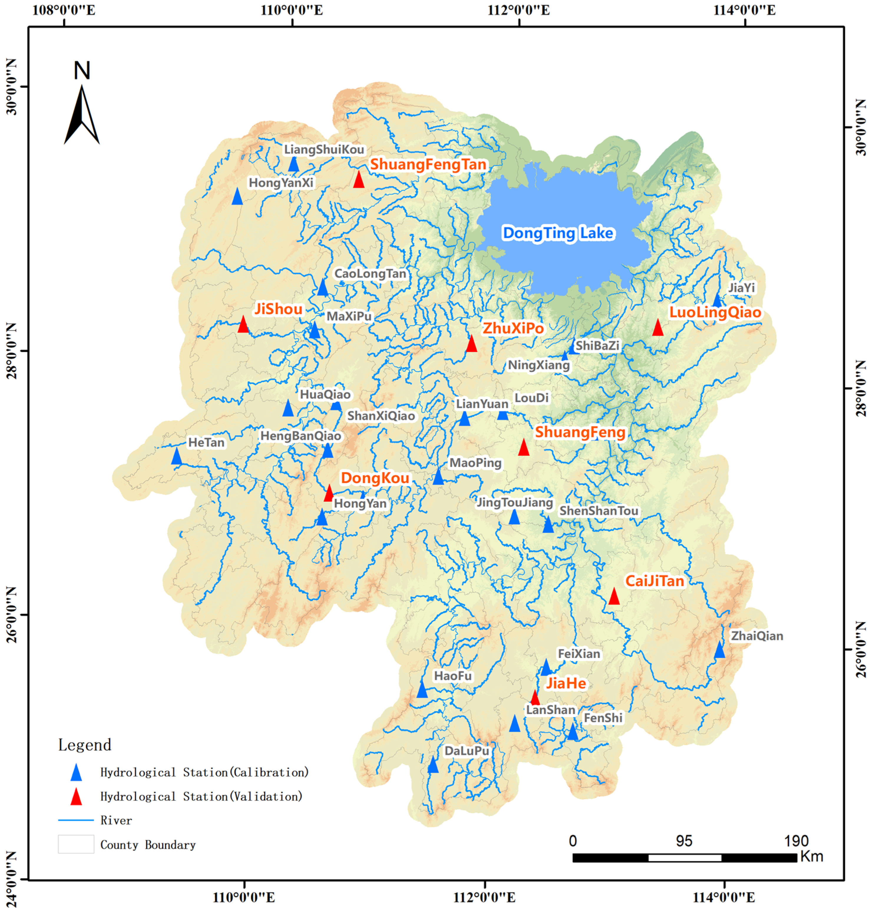
Hunan Province is located on the South Bank of the middle reaches of the Yangtze River. The general geomorphological characteristics are that it is surrounded by mountains in the east, south and west, hills in the middle, plains and lakes in the north, and an asymmetric horseshoe basin that was high in the southwest and low in the northeast. XueFeng mountain runs through the central part of the province from southwest to northeast, which divides the whole province into two parts: mountainous area and hilly area. Due to the comprehensive influence of monsoon circulation and the geomorphic conditions, the mid subtropical monsoon humid climate with obvious continental characteristics is formed. Mountain torrents occur frequently because of the complex topography, developed water system and abundant rainfall. The average annual precipitation in Hunan Province is 1450 mm, but the distribution of precipitation is uneven in time and space, and the interannual variation is large, with an average annual variation of 1200–1800 mm. The province’s annual average water surface evaporation is 736.5 mm, with a variation range of 600–900 mm.

2.2. Data Collection

Taking 33 hydrological stations with observation data from 1979 to 2020 in Hunan Province as examples, we collected the ASTER GDEM V2 dataset, land use layer and soil type layer in Hunan Province. At the same time, a distributed hydrological model of all hydrological stations was established with 30 min as the simulation step. In this study, 426 floods in 25 catchments were selected to calibrate the model parameters, and the regionalization scheme was determined by comparing the simulation results of the other 8 catchments. Figure 1 shows the distribution of hydrological stations.

The smallest catchment is HengBanQiao, with a catchment area of 31 km², and the largest catchment is FeiXian, with a catchment area of 3659 km². The hydrological data collection is shown in

Table 1. Information of study stations.

Station Name	Area (km2)	Data Years	Number of Floods	Number of Rain Stations	Number of Sub Basins	Type
NingXiang	2250	2013–2020	18	65	174	calibration
ShiBaZi	564	2013–2020	18	17	50	calibration
FeiXian	3659	2013–2020	28	157	257	calibration
FenShi	923	2013–2020	24	27	69	calibration
ZhaiQian	392	2015–2020	8	11	31	calibration
JingTouJiang	173	2014–2019	4	9	14	calibration
ShenShanTou	2930	2014–2019	5	71	227	calibration
CaoLongTan	350	2013–2015	6	7	22	calibration
HeTan	445	2014–2020	7	13	34	calibration
HengBanQiao	40	2014–2020	13	5	2	calibration
HuaQiao	81	2013–2020	22	6	5	calibration
MaXiPu	342	2012–2020	24	4	25	calibration
ShanXiQiao	1211	2013–2020	12	24	82	calibration
LianYuan	154	1979–2020	39	17	11	calibration
LouDi	1556	2014–2020	17	58	112	calibration
HongYan	711	2014–2019	8	17	55	calibration
HuangQiao	2689	2012–2019	14	76	211	calibration
SheBu	1434	2013–2020	9	38	109	calibration
MaoPing	2114	2014–2020	9	54	163	calibration
HongYanXi	190	2012–2020	20	4	11	calibration
DaLuPu	635	2013–2020	29	18	47	calibration
HaoFu	440	2013–2020	26	10	35	calibration
LanShan	305	2013–2020	32	25	19	calibration
JiaYi	1475	2013–2020	16	32	96	calibration
LiangShuiKou	865	2012–2020	18	17	65	calibration
LuoLingQiao	340	2012–2020	16	21	30	verification
JiaHe	1501	2012–2020	31	58	103	verification
CaoJiTan	387	2013–2020	13	9	30	verification
ShuangFeng	1552	2014–2020	10	36	115	verification
DongKou	928	2013–2020	13	18	66	verification
JiShou	788	2012–2020	26	30	56	verification
ZhuXiPo	699	2013–2020	15	18	53	verification
ShuangFengTan	444	2013–2020	12	20	35	verification

.

2.3. Modeling Approaches

2.3.1. Distributed Hydrological Model

Based on the ASTER GDEM V2 dataset, the sub basin and river are extracted by GIS tools. The resolution of the DEM data grid is 30 m, and the area of the sub basin is controlled within 10–30 km². At the same time, the attributes of sub basins and rivers are extracted, including basin area, slope, longest concentration path, average altitude, average drop (average elevation minus outlet elevation), river length, river section gradient, geomorphic unit hydrograph, etc.

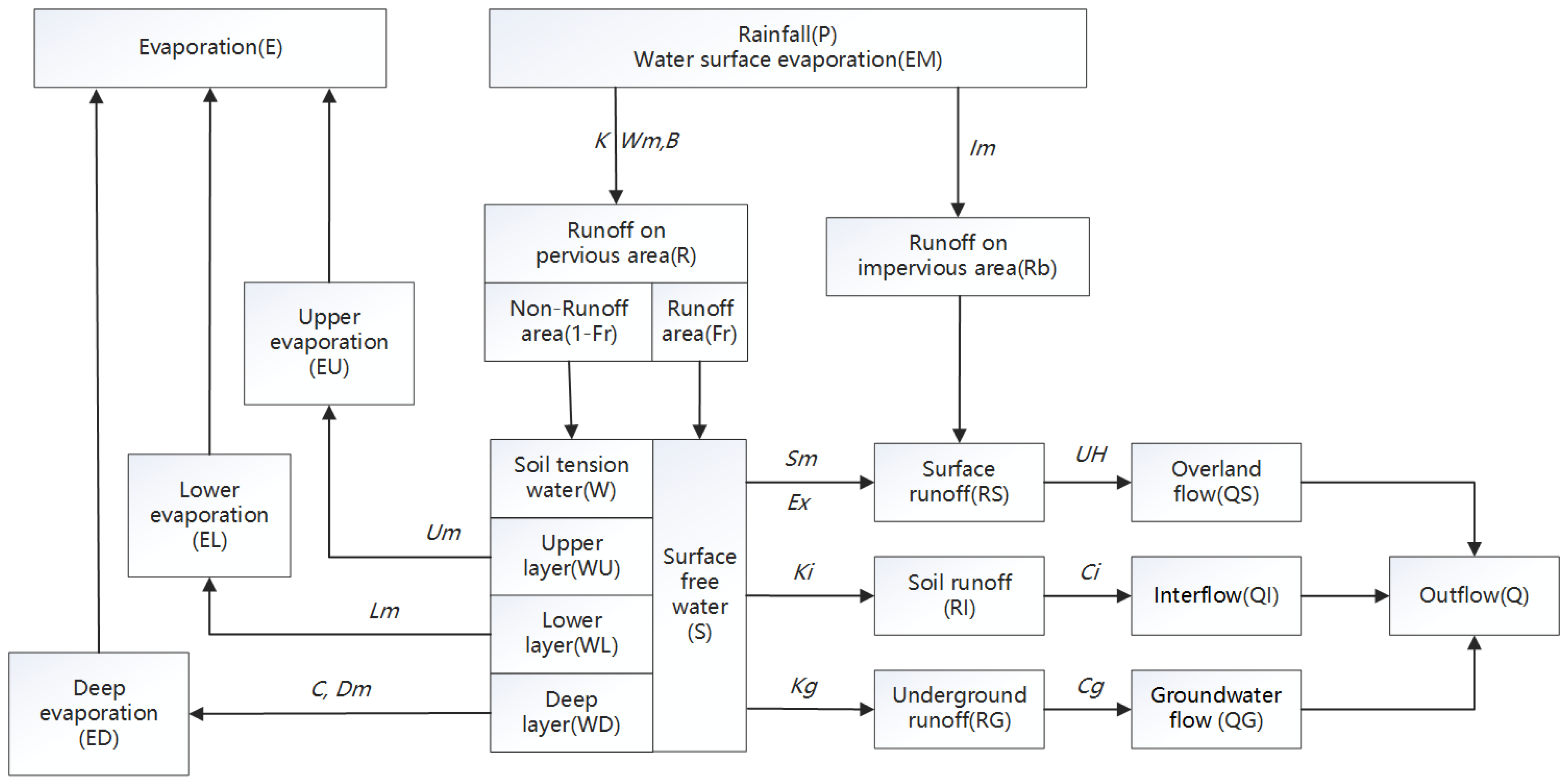
The Xinanjiang model is adopted for runoff generation computation [13,14,15]. A three-layer evaporation model is used to calculate watershed evaporation. The total runoff produced by rainfall is computed according to the concept of saturated runoff, and the influence of the uneven underlying surface on runoff yield area is considered by the water storage curve of the basin. In the aspect of runoff component division, according to the runoff production theory of “hillside hydrology”, the total runoff is divided into saturated surface runoff, soil water runoff and groundwater runoff by a reservoir with limited volume, a side hole and a bottom hole. The unit hydrograph is used to convert the surface runoff into the overland flow, and the linear reservoir model is used to calculate the interflow and groundwater flow, and is finally incorporated into the river network. Figure 2 shows the structure of the Xinanjiang model.

Table 2. Physical meanings and units of model parameters.

	Parameter	Physical Description	Unit	Param Range
1	K	Ratio of potential evapotranspiration to pan evaporation	[-]	0.5–1.2
2	Um	Averaged soil moisture storage capacity of the upper layer	[mm]	10–40
3	Lm	Averaged soil moisture storage capacity of the lower layer	[mm]	50–90
4	Dm	Averaged soil moisture storage capacity of the deep layer	[mm]	10–80
5	C	Coefficient of the deep layer that depends on the proportion of the basin area covered by vegetation with deep roots	[-]	0.1–0.3
6	B	Exponential parameter with a single parabolic curve, which represents the non-uniformity of the spatial distribution of the soil moisture storage capacity over the catchment	[-]	0.1–0.9
7	Im	Percentage of impervious and saturated areas in the catchment	[-]	0.0–1.0
8	Sm	Areal mean free water capacity of the surface soil layer, which represents the maximum possible deficit of free water storage	[mm]	10–80
9	Ex	Exponent of the free water capacity curve influencing the development of the saturated area	[-]	0.1–2.0
10	Kg	Outflow coefficients of the free water storage to groundwater relationships	[-]	0.1–0.5
11	Ki	Outflow coefficients of the free water storage to interflow relationships	[-]	0.1–0.5
12	Ci	Recession constants of the lower interflow storage	[-]	0.1–0.99
13	Cg	Recession constants of the groundwater storage	[-]	0.5–0.999

shows the parameters of the Xinanjiang model, all of which need to be determined through parameter calibration.

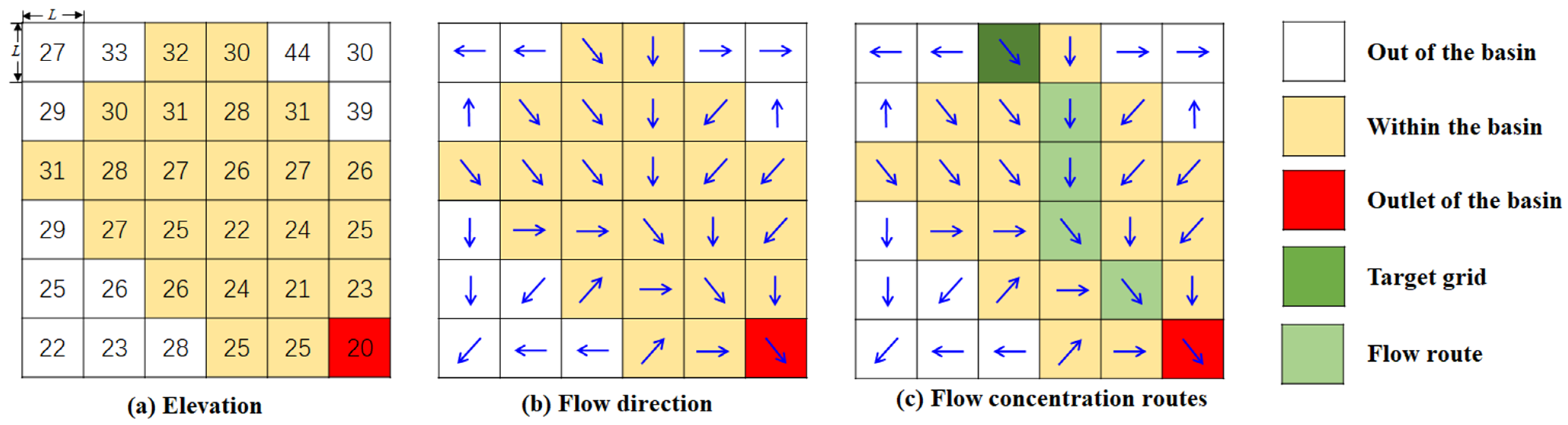
The geomorphic unit hydrograph model is adopted for overland flow concentration computation, which is based on the results of DEM data analysis (Figure 3).

The flow direction of each grid is analyzed according to the D8 algorithm [16], and the probability density distribution function of concentration time is determined by computing the time of each water particle falling on the surface of the basin reaching the outlet, so as to further determine the geomorphic unit hydrograph [17]. Based on the principle of energy conversion, this improves the formula of flow velocity and unifies the formula of slope velocity and river velocity [18], as shown in Formula (1).

$$v=\sqrt{\frac{2{\mu }^{\prime }g {{\displaystyle \sum }}_{k=1}^{n}sin\frac{{\theta }_k}{2}{n}_k\Delta h_k }{n}}$$

(1)

where μ′ is the energy residual coefficient and its range is [0,1], θ is the slope angle of the grid outflow direction, n is the total number of grids in the basin upstream of the target grid (including the target grid), g is the gravity acceleration, Δh is the elevation difference between the target grid and the outflow grid, N is the number of inflow grids of the target grid, n_k and v_k are the number of upstream grids and the average flow velocity of the kth inflow grid, respectively.

The Muskingum model is used for river network flow concentration [19,20]. Continuous flood routing is realized by segment-by-segment estimation of the model parameters [21].

2.3.2. Evaluation Criteria

To evaluate the suitability of the proposed model for the studied Basin, the Nash–Sutcliffe Coefficient of Efficiency (NSCE) is chosen to analyze the degree of goodness of fit [22], which is defined as:

$$NSCE=1-\frac{{{\displaystyle \sum }}_{i=1}^N{\left(Q_s\left(i\right)-Q_0\left(i\right)\right)}^2}{{{\displaystyle \sum }}_{i=1}^N{\left(Q_0\left(i\right)-\overline{Q}\right)}^2}$$

(2)

where Q_o(i) and Q_s(i) are the observed and simulated flow, respectively, N is the number of data points, and $\overline{Q}$ is the mean value of the observed flow. According to national criteria for flood forecasting in China [23], the scheme is excellent when the average NSCE reaches 0.9. When the average NSCE is greater than 0.7 and less than 0.9, the effect of this scheme is better. This scheme is for reference only; if the average NSCE is greater than 0.5 but less than 0.7, it may not be accurate. Otherwise, the results of the performances of parameter calibration are unsatisfactory for online flood forecasting.

2.3.3. Parameter Optimization Method

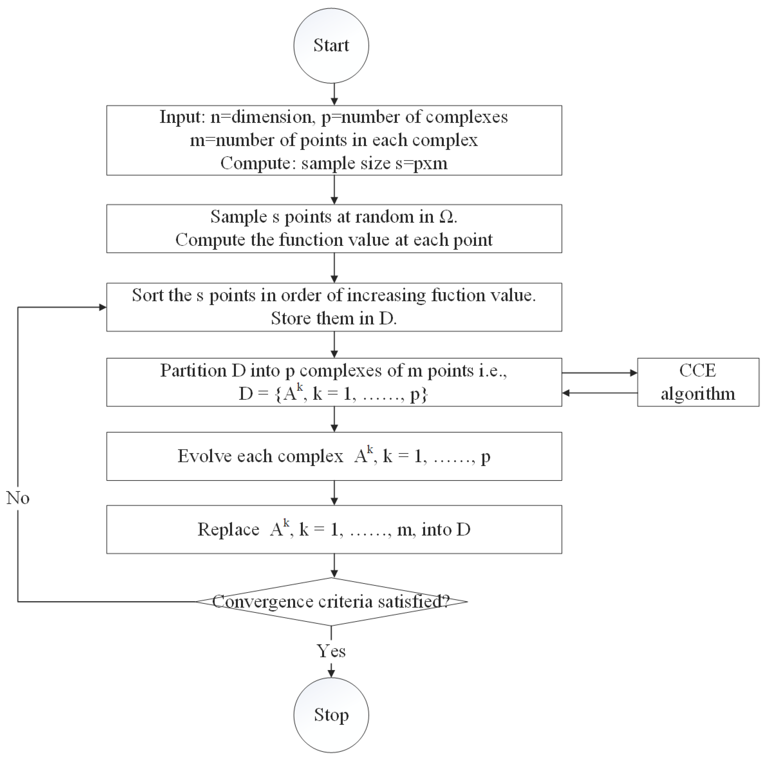
The shuffled complex evolution (SCE-UA) method is used to optimize the model parameters. The SCE-UA algorithm is a nonlinear hybrid algorithm which combines the advantages of the genetic algorithm and the simplex algorithm, and is based on information exchange and biological evolution laws. It can effectively solve the problems of multi-peak, multi-noise, discontinuity, high-dimension and non-linearity in parameter optimization. Figure 4 shows the calculation flow of the SCE-UA algorithm. This method can efficiently and quickly search for the global optimal solution of model parameters [24,25]. There are 14 parameters that need to be optimized in this study, including 13 parameters of the Xinanjiang model (see Table 1) and 1 parameter of the geomorphic unit hydrograph (μ′). μ′ is the energy residual coefficient and its range is [0,1].

According to the evaluation criteria, the larger the NSCE, the better the simulation effect. Therefore, this study aimed to find the highest mean value of NSCE. Since the goal of the SCE-UA algorithm is to find the minimum, Equation (3) is used as the objective function.

$$F=1-\frac{{{\displaystyle \sum }}_{i=1}^{t}NSC{E}_i}{t}$$

(3)

where F is the value of objective function, t is the number of floods.

2.3.4. Parameter Regionalization Scheme

The Shortest Distance, Attribute Similarity, Support Vector Regression, Generative Adversarial Networks, Classification and Regression Tree and Random Forest method are used to determine the parameter regionalization scheme, and the final scheme is determined by comparing the simulation results of different methods. For readability,

Table 3. Abbreviation of parameter regionalization methods.

Abbreviation	Method Name	Abbreviation	Method Name
SD	shortest distance	GAN	generative adversarial networks
AS	attribute similarity	CART	classification and regression tree
SVR	support vector regression	RF	random forest

lists the abbreviations representing the different methods.

(1)

Shortest Distance (SD)

The nearest basin is determined by computing the spatial distance between the centroid coordinates of the study basin and other basins, and the model parameters of the nearest basin are directly applied to the distributed model of the study basin.

$$D=2R{\sin }^{-1}\sqrt{sin{\left(\frac{Lat1-Lat2}{2}\right)}^2+cos\left(Lat1\right)cos\left(Lat2\right)sin{\left(\frac{Lon1-Lon2}{2}\right)}^2}$$

(4)

where D is the distance, R is the radius of the earth, about 6,378,137 m, and Lon1, lat1, lon2 and Lat2 are the centroid coordinates of the two basins.

(2)

Attributes Similarity (AS)

The area (A, km²), average slope (P), average elevation (E, m), average elevation drop (H, m), shape coefficient (L), soil type S = {s₁, s₂, s₃} (s₁, s₂ and s₃ are the percentages of clay, silt and sand, %) and land use U = {u₁, u₂, u₃, u₄} (u₁, u₂, u₃, u₄ are the percentages of forest, grass, cultivated land and other, %) were selected for similarity analysis. The components of U and S range in value from 0 to 1, so no additional processing is required. However, for other attributes, the maximum value method is used for normalization, as follows: collect the maximum values MaxA, MaxP, MaxE, MaxH and MaxL of attribute A, P, E, H and L in 33 catchments, and then let C = {A/MaxA, P/MaxP, E/MaxE, H/MaxH, L/MaxL}, then C is the normalized result. The similarity index of catchment x and catchment y was defined as Formula (5):

$$T=\frac{\cos \left(S_x, S_y\right)+\cos \left(U_x, U_y\right)+1-D\left(C_x, C_y\right) }{3}$$

(5)

where D(a,b) and cos(a,b) are Euclidean distances and cosines value of two vectors a and b, respectively.

$$D\left(a,b\right)=\sqrt{{{\displaystyle \sum }}_{i=1}^n{\left(a_i-b_i\right)}^2}$$

(6)

$$\cos \left(a, b\right)=\frac{{{\displaystyle \sum }}_{i=1}^n{a}_i{b}_i}{\sqrt{{{\displaystyle \sum }}_{i=1}^n{a_i}^2}\sqrt{{{\displaystyle \sum }}_{i=1}^n{b_i}^2}}$$

(7)

where T is the similarity index, and its range is [0,1]. The larger the T value, the greater the similarity between the two catchments. Select the basin most similar to the study basin and transplant its parameters.

(3)

Support Vector Regression (SVR)

The essence of a support vector machine (SVM) is to map the non-linear function relationship to the linear problem of high-dimensional space, and then find the optimal regression hyperplane in this high-dimensional space, so that all samples are the minimum distance from the optimal hyperplane [26]. Support Vector Regression (SVR) is a method based on a support vector machine to deal with regression problems. It is used to study the relationship between input variables and numerical output variables, and to predict the output value of new variables. It retains the advantages of a support vector machine and is mainly used in the case of a limited or small number of samples [27].

(4)

Generative Adversarial Network (GAN)

The generative adversarial network (GAN) is an unsupervised learning model consisting of a discriminator and a generator [28]. The generator automatically generates data, learns the distribution of real samples, and generates pseudo samples that are close to real samples. The discriminator has to distinguish between real samples obtained from the data and fake samples generated by the generator. The two models are iteratively optimized through continuous confrontation training, so that the data distribution generated by the generator is as close as possible to the real data distribution. When the probability of each output of the discriminator is basically 1/2, it indicates that the model has reached the optimal state.

(5)

Classification And Regression Tree (CART)

The CART (Classification and Regression Tree) algorithm is a decision tree classification method. It uses a dichotomy recursive segmentation technique to divide the current sample set into two sub sample sets, so that each non leaf node generated has two branches. The decision tree is a weak learning algorithm [29]. The improvement of classification accuracy depends on the reasonable construction and pruning of the tree structure. The CART algorithm generates a decision tree based on the training dataset, and the generated decision tree should be as large as possible. The validation dataset is used to prune the generated tree and select the optimal subtree. At this time, the minimum loss function is used as the pruning standard.

(6)

Random Forest (RF)

Random forest model generates multiple different datasets from the original dataset by sampling with put back [30]. The CART tree is used as a weak classifier, and each sub-dataset corresponds to a classifier. Each decision tree selects the attribute with the strongest classification ability for node splitting, without pruning to maximize growth. All final generated decision trees form a random forest. The model can be used for classification or regression prediction, the result of which is determined by the classifier voting.

Based on the above, Figure 5 shows the flow of parameter regionalization. When SVR, GAN, CART and RF are selected for parameter transplantation. The analysis steps are as follows:

(1)

For each calibrated catchment A, use the model parameters of any catchment B to compute the average Nash–Sutcliffe coefficient NSCE_a-b. Collect all catchment A attributes, catchment B attributes, NSCE_a-b as training dataset for model training. In this study, the sample size of the training set is 25 × 25.

(2)

For each verified catchment C and calibrated catchment D, use the trained model to take the attributes of C and D as input to predict the mean NSCE, and the parameter group with the highest predictive value is used as the model parameter of C.

3. Results

3.1. Model Parameter Optimization

The SCE-UA algorithm is used to automatically optimize the model parameters of 25 hydrological stations, and the objective function is to obtain the highest average Nash–Sutcliffe coefficient. The results of parameter calibration are shown in

Table 4. Simulation results of calibration.

Station	NSCE	Station	NSCE	Station	NSCE
NingXiang	0.78	HengBanQiao	0.80	MaoPing	0.77
ShiBaZi	0.76	HuaQiao	0.61	SheBu	0.83
FeiXian	0.79	MaXiPu	0.72	HongYanXi	0.83
FenShi	0.84	ShanXiQiao	0.79	DaLuPu	0.82
ZhaiQian	0.77	LianYuan	0.86	HaoFu	0.80
JingTouJiang	0.87	LouDi	0.78	LanShan	0.67
ShenShanTou	0.83	HongYan	0.74	JiaYi	0.86
CaoLongTan	0.85	HuangQiao	0.74	LiangShuiKou	0.87
HeTan	0.79

.

It can be seen that there are 23 hydrological stations with an average NSCE between 0.7 and 0.9, and 2 between 0.5 and 0.7. According to national criteria for flood forecasting in China, most calibration parameters meet the requirements of online flood forecasting. The distributed model based on the Xinanjiang model and geomorphic unit hydrograph is stable and suitable for most areas of Hunan Province.

The calibration parameters were fed into the distributed model to simulate 426 floods in 25 catchments. Taking LianYuan Station as an example, the calibration result is shown in Figure 6.

3.2. Regionalization Schemes

The shortest distance, attribute similarity, support vector regression, generative adversarial networks, classification and regression tree, and random forest models are selected to construct and verify the parameter regionalization scheme.

According to the catchment attributes, the results of SD and AS can be directly calculated. The centroid coordinates and basic attributes of the 33 catchments are shown in

Table 5. Information of typical watershed characteristics.

Station Name	Centroid Coordinates		Basic Attributes					Land Use (%)				Soil Type (%)
	lon	lat	A (km2)	P	E (m)	H (m)	L	u1	u2	u3	u4	s1	s2	s3
NingXiang	112.2487	28.0972	2250	0.160	167.36	145.36	0.208	49.8	1.9	42.4	5.9	44.3	55.5	0.2
ShiBaZi	112.3625	28.0153	564	0.125	113.57	77.57	0.289	45.2	1.4	49.6	3.8	42.3	57.7	0.0
FeiXian	112.2963	25.6634	3559	0.213	395.16	261.16	0.244	49.8	5.5	38.3	6.4	18.3	74.9	6.8
FenShi	112.5636	25.2776	923	0.241	500.12	287.12	0.380	59.4	5.0	29.0	6.6	31.5	68.2	0.3
ZhaiQian	113.9350	26.0667	392	0.345	1140.59	428.59	0.629	87.8	5.2	2.7	4.3	16.8	83.2	0.0
JingTouJiang	112.0796	26.9399	173	0.181	227.96	118.96	1.113	57.7	1.7	38.9	1.7	64.1	35.9	0.0
ShenShanTou	112.2196	27.0911	2930	0.176	175.06	134.06	0.131	49.0	1.6	45.9	3.5	47.0	53.0	0.0
CaoLongTan	110.4173	28.8383	350	0.457	533.01	434.01	0.093	95.3	0.2	3.6	0.9	31.9	68.1	0.0
HeTan	109.1290	27.1854	445	0.372	616.32	274.32	0.391	84.4	4.0	10.1	1.5	90.1	9.9	0.0
HengBanQiao	110.5267	27.3562	31	0.323	757.67	274.67	0.424	89.5	1.2	8.5	0.8	61.1	38.9	0.0
HuaQiao	110.2038	27.6833	81	0.279	500.44	314.44	2.249	86.6	0.8	11.7	0.9	86.5	13.5	0.0
MaXiPu	110.4492	28.2416	342	0.383	386.66	297.66	0.119	88.6	0.8	9.3	1.3	87.7	12.2	0.1
ShanXiQiao	110.5982	27.5358	1211	0.342	803.06	651.06	0.173	86.6	3.6	8.3	1.5	64.0	36.0	0.0
LianYuan	111.6015	27.6335	154	0.229	248.27	128.27	0.508	54.1	2.7	36.8	6.4	59.0	41.0	0.0
LouDi	111.7627	27.8257	1556	0.236	312.35	239.35	0.220	52.6	4.6	35.3	7.5	61.9	36.0	2.1
HongYan	110.3664	26.8192	711	0.294	634.08	303.08	0.302	78.7	1.1	18.5	1.7	66.4	33.6	0.0
HuangQiao	110.5639	26.7795	2689	0.226	515.43	274.43	0.268	58.3	1.4	37.1	3.2	30.5	69.3	0.2
SheBu	111.6256	27.1677	2114	0.155	322.56	137.56	0.233	38.1	3.9	51.3	6.7	42.9	57.1	0.0
MaoPing	112.5982	27.4498	1434	0.164	154.98	122.98	0.298	58.9	0.8	38.0	2.3	23.1	76.9	0.0
HongYanXi	109.5954	29.3404	190	0.367	689.85	322.85	0.393	84.2	1.4	13.9	0.5	42.8	57.2	0.0
DaLuPu	111.5408	24.8728	635	0.232	487.37	269.37	0.223	54.0	5.3	35.6	5.1	18.8	80.4	0.8
HaoFu	111.4058	25.7095	440	0.328	565.82	365.82	0.528	77.5	1.7	19.1	1.7	58.4	41.6	0.0
LanShan	112.1479	25.2640	305	0.340	675.70	428.70	0.352	82.7	1.2	12.0	4.1	54.8	45.2	0.0
JiaYi	113.9674	28.7773	1475	0.274	316.37	248.37	0.276	77.5	2.5	17.0	3.0	44.6	55.4	0.0
LiangShuiKou	110.0255	29.6915	865	0.471	778.04	496.04	0.338	94.2	0.2	5.4	0.2	32.3	67.7	0.0
LuoLingQiao	113.3727	28.5341	340	0.170	113.07	77.07	0.652	65.2	1.2	29.9	3.7	70.0	30.0	0.0
JiaHe	112.2656	25.3685	1501	0.263	511.87	337.87	0.276	66.2	2.7	26.1	5.0	36.8	54.3	8.9
CaoJiTan	113.1137	26.3820	387	0.197	179.50	90.50	0.352	63.2	1.5	32.5	2.8	50.7	44.6	4.7
ShuangFeng	112.0508	27.4016	1552	0.164	175.11	118.11	0.301	40.4	2.9	51.6	5.1	20.5	79.5	0.0
DongKou	110.4491	27.1576	928	0.362	756.60	458.60	0.454	93.5	0.8	4.9	0.8	56.5	43.5	0.0
JiShou	109.5497	28.3203	788	0.356	621.50	453.50	0.208	81.5	3.0	14.0	1.5	58.3	41.7	0.0
ZhuXiPo	111.6941	28.1490	699	0.353	422.86	310.86	0.450	81.3	2.1	14.4	2.2	90.0	8.3	1.7
ShuangFengTan	110.5954	29.3742	444	0.360	591.95	446.95	0.257	87.0	0.6	11.2	1.2	66.1	32.5	1.4

, including east longitude (lon, ◦), north latitude (lat, ◦), area (A, km²), average slope (P), average elevation (E, m), average elevation drop (H, m), shape coefficient (L), and the percentages of forest (u₁), grass (u₂), cultivated land (u₃), other (u₃), clay (s₁), silt (s₂) and sand (s₃). These attributes were extracted during sub-watershed division.

According to the coordinates of the center of the basin, the centroid distance between the verification basin and the calibration basin is calculated by Formula (3), and the calibration basin with the closest distance is selected, and its model parameters are used directly. Normalize the basin properties, calculate the similarity index between the verification basin and the calibration basin using Formula (4), and transfer the model parameters with the highest similarity.

Table 6. Transplant results of SD and AS methods.

Station Name	SD		AS
	Transplant Station	NSCE	Transplant Station	NSCE
LuoLingQiao	JiaYi	0.66	LianYuan	0.86
JiaHe	LanShan	0.69	JiaYi	0.31
CaoJiTan	ZhaiQian	0.27	LianYuan	0.61
ShuangFeng	ShenShanTou	0.75	MaoPing	0.74
DongKou	HengBanQiao	0.29	HaoFu	0.72
JiShou	MaXiPu	0.71	ShanXiQiao	0.46
ZhuXiPo	LouDi	0.60	HeTan	0.72
ShuangFengTan	CaoLongTan	0.64	HongYan	0.69
Average Value		0.58		0.64

shows the transplant results of the SD and AS methods.

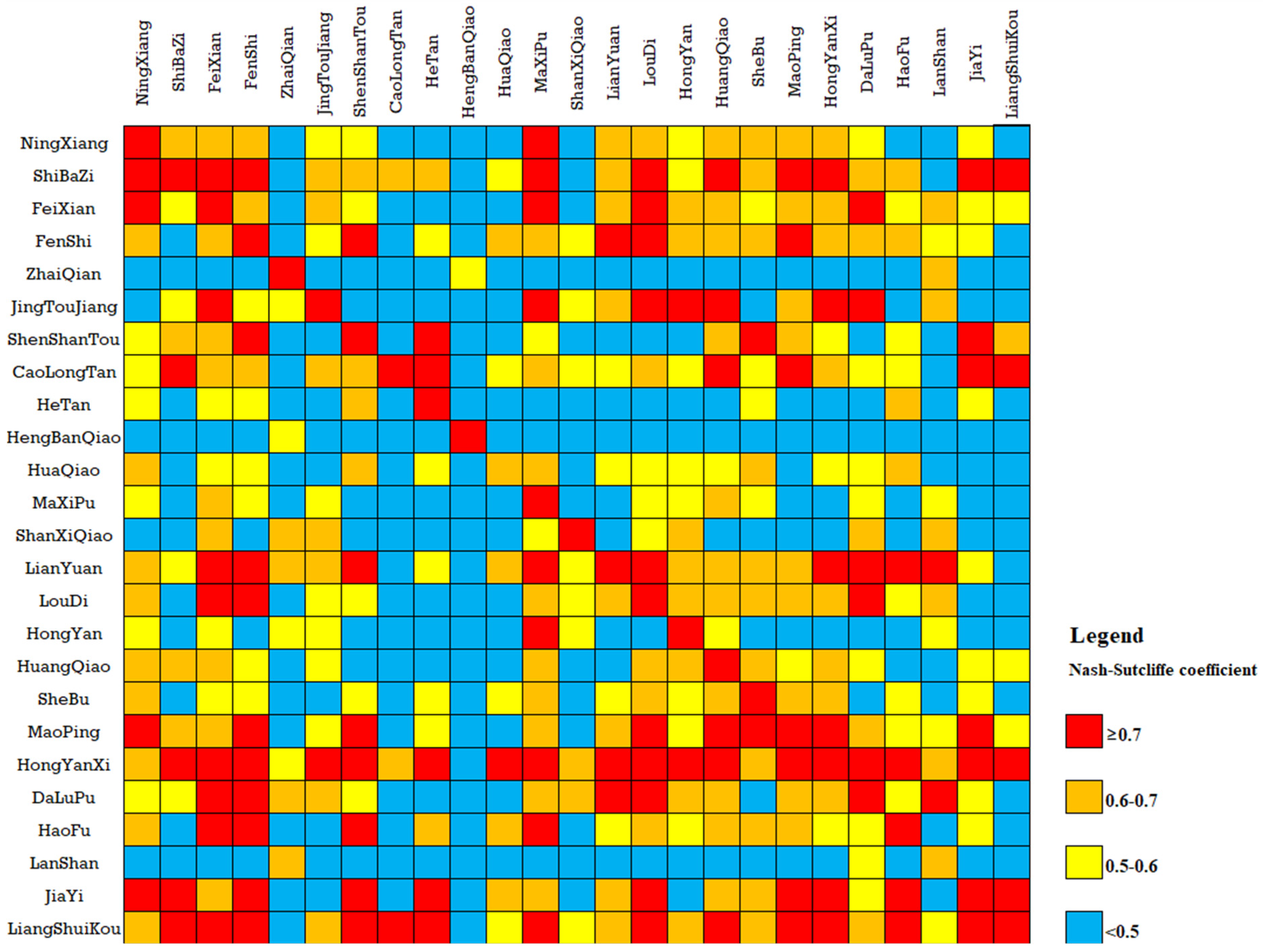
For SVR, GAN, CART and RF methods, we need to collect samples and train the model first. This required cross-validation of the model parameters for 25 catchments. We apply 25 groups of parameters to the flood simulations of 25 catchments and calculate the mean NSCE.

Figure 7 shows the 25 × 25 cross-validation results for the samples. Among the 625 samples, there are 121 samples with a Nash–Sutcliffe coefficient greater than 0.7, accounting for 19.4% of the total number of samples; 138 samples with a Nash–Sutcliffe coefficient between 0.6 and 0.7, accounting for 22.1%; 112 samples with a Nash–Sutcliffe coefficient between 0.6 and 0.7, accounting for 17.9%; and 254 samples with a Nash–Sutcliffe coefficient less than 0.5, accounting for 40.1%. These samples are used as input to train four models of SVR, GAN, CART and RF, and the results of different parameter groups are used to predict eight verification basins, and the optimal results are selected for parameter transplantation. The Nash–Sutcliffe coefficients of the simulation results are shown in

Table 7. Transplant results of machine learning methods.

Station Name	NSCE
	SVR	GAN	CART	RF
LuoLingQiao	0.75	0.71	0.65	0.78
JiaHe	0.55	0.69	0.51	0.65
CaoJiTan	0.42	0.43	0.61	0.64
ShuangFeng	0.25	0.57	0.35	0.64
DongKou	0.80	0.78	0.80	0.65
JiShou	0.75	0.71	0.71	0.75
ZhuXiPo	0.52	0.64	0.57	0.59
ShuangFengTan	0.79	0.78	0.66	0.72
Average Value	0.60	0.66	0.61	0.68

.

4. Discussion

It can be seen from Table 6 that two groups, CaojiTan-ZhaiQian and DongKou-HengBanQiao, performed poorly when using the transplantation parameters of the SD method, with average NSCE of 0.27 and 0.29, respectively. When the AS method was used for transplant parameters, two groups had poor results, namely JiaHe-JiaYi and JiShou-ShanXiQiao, with average NSCEs of 0.31 and 0.46, respectively.

Table 8. Information on basin attributes.

Station Name		CaoJiTan	ZhaiQian	DongKou	HengBanQiao	JiaHe	JiaYi	JiShou	ShanXiQiao
Basin Attributes	Area (km2)	387	392	928	31	1501	1475	788	1211
	Average Slope	0.197	0.345	0.362	0.323	0.263	0.274	0.356	0.342
	Average Elevation (m)	179.5	1140.59	756.6	757.67	511.87	316.4	621.5	803.1
	Average Elevation Drop (m)	90.5	428.59	458.6	274.67	337.87	248.4	453.5	651.1
	Shape Coefficient	0.352	0.629	0.454	0.424	0.276	0.276	0.208	0.173
Land Use (%)	Forest	63.2	87.8	93.5	89.5	66.2	77.5	81.5	86.6
	Grass	1.5	5.2	0.8	1.2	2.7	2.5	3	3.6
	Cultivated Land	32.5	2.7	4.9	8.5	26.1	17	14	8.3
	Other	2.8	4.3	0.8	0.8	5	3	1.5	1.5
Soil (%)	Clay	50.7	16.8	56.5	61.1	36.8	44.6	58.3	64
	Silt	44.6	83.2	43.5	38.9	54.3	55.4	41.7	36
	Sand	4.7	0	0	0	8.9	0	0	0

shows the attributes of these groups of catchments.

It can be seen from Table 8 that DongKou and HengBanQiao are not only close, but also most of the attributes are similar except for the area and average drop. The area of DongKou is 931 km², and the area of HengBanQiao is 31 km². Their average drops are 458.6 m and 274.67 m, respectively. It is obvious that the different areas will lead to large differences in concentration time, and the average drop may significantly affect the concentration speed, which is the most critical factor affecting the geomorphic unit hydrograph [18]. Similarly, compared with JiaHe and JiaYi, their attributes are very similar, except for average elevation and drop. Therefore, we can infer that if the attributes of two catchments are very close, but their average drop difference is significant, this is likely to cause a failed transplantation. The opposite conclusion cannot be established. Table 6 shows an example with the best results (LuoLingQiao-LianYuan). The average NSCE of transplantation can reach 0.86, which is excellent according to the evaluation criteria. However, the attributes of the two catchments, including the average drop, differed significantly (as shown in Table 5).

From the above cases, it can be seen that the applicable conditions and scope of parameter transplantation are relatively complex, and a single factor cannot be considered in isolation. When multiple attributes are considered for parameter transplantation, the results may not be satisfactory for catchments with similar attributes sometimes, so precisely defining the similarity index is a challenge.

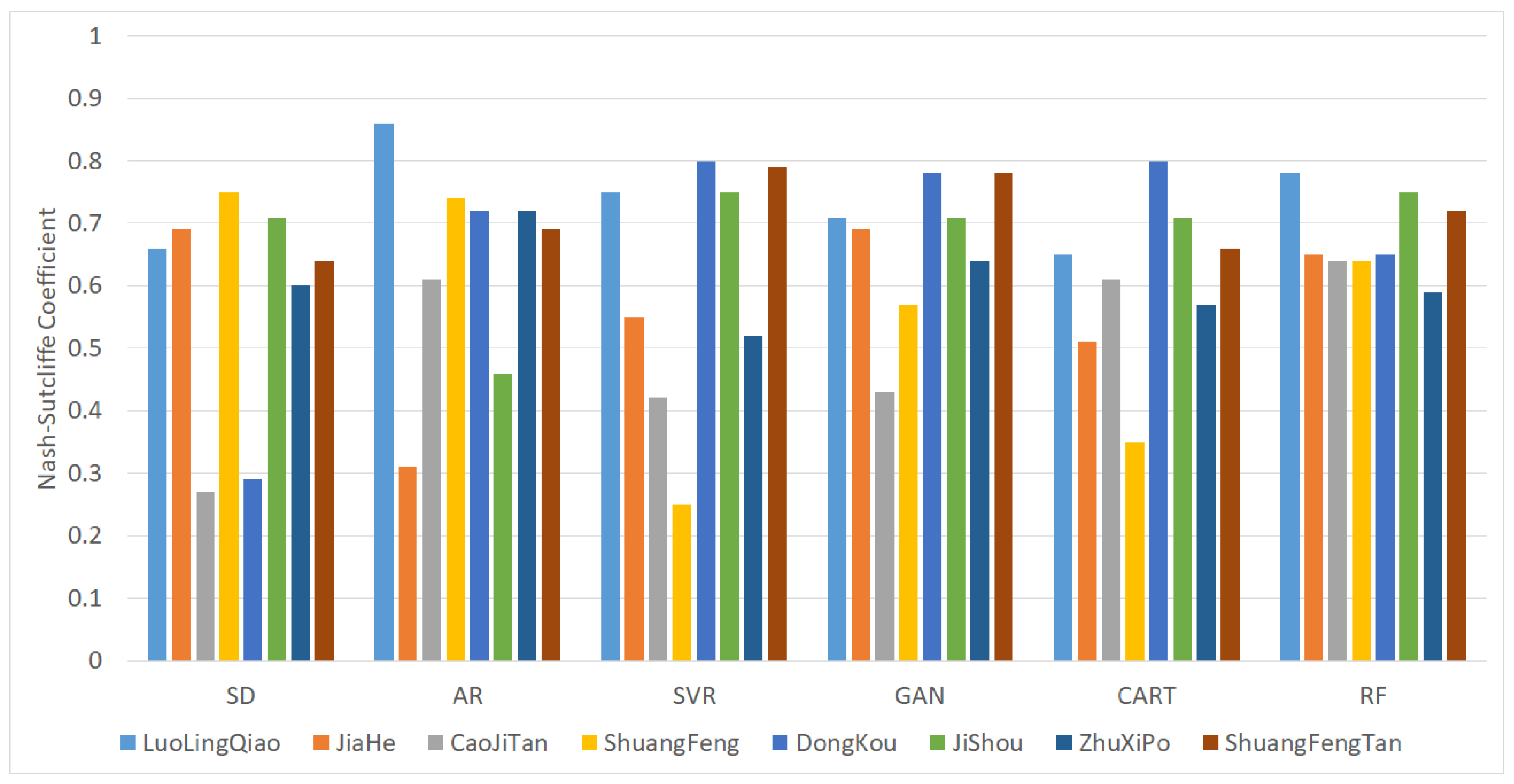
In contrast, machine learning methods can discover more hidden rules in data. However, the methods of machine learning cannot all achieve satisfactory results. Comparing only the average NSCE, the results of SVR and CART were even worse than the AS method. In order to better compare the performance of different methods,

Table 9. Comparison of parameter regionalization schemes.

Items	NSCE
	SD	AR	SVR	GAN	CART	RF
Best	0.75	0.86	0.80	0.78	0.80	0.78
Worst	0.27	0.31	0.25	0.43	0.35	0.59
Average	0.58	0.64	0.60	0.66	0.61	0.68

shows the optimal value, worst value and average value obtained using different methods. Figure 8 shows the average NSCEs for the different methods.

It can be seen from Table 9 that the average and worst Nash–Sutcliffe coefficients of the simulation results using the random forest model are the highest. Among the best NSCE results in Table 9, AR > SVR ≥ CART > RF ≥ GAN > SD, with AR performing best and SD performing worst. The worst result of NSCE is RF > GAN > CART > AR > SD > SVR; RF is the best and SVR is the worst. According to the NSCE average results, RF > GAN > AR > CART> SVR > SD; RF performed the best and SD performed the worst.

Table 10. NSCE statistical results.

NSCE	SD	AR	SVR	GAN	CART	RF
≥0.9	0	0	0	0	0	0
0.7–0.9	25%	50%	50%	50%	25%	37.5%
0.5–0.7	50%	25%	25%	37.5%	62.5%	62.5%
<0.5	25%	25%	25%	12.5%	12.5%	0

summarizes the validation results of the different methods and shows the percentage of catchments with an average NSCE greater than 0.9, greater than 0.7 and less than 0.9, greater than 0.5 and less than 0.7, and less than 0.5.

It can be seen from Table 10 that all of the NSCE results of RF are greater than 0.5, which is not achieved by all of the other methods. According to national criteria for flood forecasting in China, if the average NSCE is less than 0.5, the simulation result is unsatisfactory for online flood forecasting. Therefore, the RF model has better performance than the other methods.

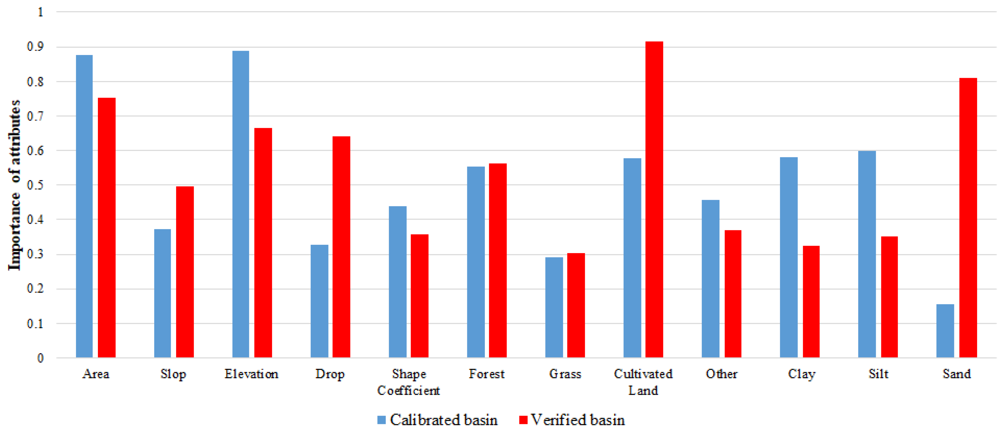
Figure 9 lists the importance of each attribute in the RF model. The most important attribute for prediction using the RF model is the percentage of cultivated land area within the transplanted catchment, followed by the area and average elevation of the calibration catchment. It is well known that slope is a significant impact on hydrological models. However, from the parameter importance of the RF model, the influence of slope is smaller than that of cultivated land, which may be another issue that needs further research.

5. Conclusions

In this study, the distribution hydrological models of 33 small and medium-sized catchments in Hunan Province were constructed. The model parameters of 25 catchments were calibrated by using the SCE-UA algorithm. The parameter regionalization scheme including Shortest Distance (SD), Attribute Similarity (AS), Support Vector Regression (SVR), Generative Adversarial Networks (GAN), Classification and Regression Tree (CART) and Random Forest (RF) were validated using data from eight catchments. The main conclusions are as follows:

(1)

A total of 426 floods of 25 catchments were selected to calibrate the model parameters. Among the simulation results of these 25 catchments, there are 23 catchments with an average NSCE greater than 0.7, and 2 between 0.5 and 0.7. According to national criteria for flood forecasting in China, most calibration parameters meet the requirements of online flood forecasting. The distributed model based on the Xinanjiang model and geomorphic unit hydrograph is suitable for most areas of Hunan Province.

(2)

Based on the watershed attributes and cross validation results of model parameters, six parameter regionalization schemes including SD, AR, SVR, GAN, CART and RF were generated, and 136 floods of 8 catchments were used for verification. The average values of the Nash–Sutcliffe coefficients of each scheme were 0.58, 0.64, 0.60, 0.66, 0.61 and 0.68, and the worst values were 0.27, 0.31, 0.25, 0.43, 0.35 and 0.59. The Nash–Sutcliffe coefficients of the RF model are all greater than 0.5, which cannot be achieved by other methods. The RF model is the most stable solution and significantly outperforms other methods. Using the random forest model to regionalize parameters can improve the accuracy of flood simulation in ungauged areas, which is of great significance for flash flood forecasting and early warning.

(3)

The applicable conditions and scope of parameter transplantation are relatively complex, and a single factor cannot be considered in isolation, and the attributes of adjacent catchments may also vary greatly. The result of the attribute similarity method is not very stable, and transplantation can fail when most of the attributes of two catchments are similar, but if the attributes are very different, sometimes good results will be achieved. According to the parameter importance analyzed by the RF model, the slope is not so important, while the cultivated land area is the key to decision making. This result goes against common sense and deserves further research.

There are many factors that affect the accuracy of parameter transplantation. In practice, continuous data collection is required to improve the quality of the underlying dataset. With the accumulation of data and the continuous improvement of the regionalization model, the accuracy of parameter transplantation can be improved.

References

- Gou, J.J.; Miao, C.Y.; Duan, Q.Y. Progress in parameter sensitivity analysis-optimization-regionalization methods for hydrological models. Prog. Geogr. 2022, 41, 1338–1348. [Google Scholar] [CrossRef]
- Sivapalan, M. Prediction in ungauged basins: A grand challenge for theoretical hydrology. Hydrol. Process. 2003, 17, 3163–3170. [Google Scholar] [CrossRef]
- Young, A.R. Stream flow simulation within UK ungauged catchments using a daily rainfall-runoff model. J. Hydrol. 2006, 320, 155–172. [Google Scholar] [CrossRef]
- Parajka, J.; Bloschl, G.; Merz, R. Regional calibration of catchment models: Potential for ungauged catchments. Water Resour. Res. 2007, 43. [Google Scholar] [CrossRef]
- Li, H.X.; Zhang, Y.Q.; Chiew, F.H.S.; Xu, S. Predicting runoff in ungauged catchments by using Xinanjiang model with MODIS leaf area index. J. Hydrol. 2009, 370, 155–162. [Google Scholar] [CrossRef]
- Yokoo, Y.; Kazama, S.; Sawamoto, M.; Nishimura, H. Regionalization of lumped water balance model parameters based on multiple regression. J. Hydrol. 2001, 246, 209–222. [Google Scholar] [CrossRef]
- Cheng, X.; Ma, X.X.; Wang, W.S.; Liu, X.X.; Wang, Q.L.; Xiao, Y. Applicability Research of HEC-HMS Model Parameter Regionalization in Small Basin of Henan Province. J. China Hydrol. 2022, 42, 40–46, 102. [Google Scholar] [CrossRef]
- Yao, C.; Qiu, Z.Y.; Li, Z.J.; Hu, W.D.; Xu, J. Parameter regionalization study and application of API model and Xin’anjiang model. J. China Inst. Water Resour. Hydropower Res. 2019, 47, 189–194. [Google Scholar] [CrossRef]
- Sun, Z.L.; Liu, Y.L.; Chen, X.; Shu, Z.K.; Wu, H.F.; Wang, J.; Bao, Z.X.; Wang, G.Q. Review of Hydrological Model Parameter Regionalization Method [OL]. J. China Hydrol. 2022, 1–9. [Google Scholar] [CrossRef]
- Yi, X.; Zhou, F.; Wang, X.Y.; Yang, Y.H.; Guo, H.C. Classification and runoff simulation of data-scarce basins based on self-organizing maps. Prog. Geogr. 2014, 33, 1109–1116. [Google Scholar]
- Ragettli, S.; Zhou, J.; Wang, H.; Liu, C.; Guo, L. Modeling flash floods in ungauged mountain catchments of China: A decision tree learning approach for parameter regionalization. J. Hydrol. 2017, 555, 330–346. [Google Scholar] [CrossRef]
- Liu, C.J.; Zhou, J.; Wen, L.; Ma, Q.; Guo, L.; Ding, L.Q.; Sun, D.Y. Research on spatio temporally-mixed runoff model and parameter regionalization for small and medium-sized catchments. J. China Inst. Water Resour. Hydropower Res. 2021, 19, 99–114. [Google Scholar] [CrossRef]
- Zhao, R.J. The Xinanjiang model applied in China. J. Hydrol. 1992, 135, 371–381. [Google Scholar] [CrossRef]
- Zhao, R.J.; Zhang, Y.L.; Fang, L.R. The Xinanjiang model. In Hydrological Forecasting, Proceeding Oxford Symposium, Oxford, UK, 15–18 April 1980; IASH: Washington, DC, USA, 1980; pp. 351–356. [Google Scholar]
- Wang, W.C.; Cheng, C.T.; Chau, K.W.; Xu, D.M. Calibration of Xinanjiang model parameters using hybrid genetic algorithm based fuzzy optimal model. J. Hydroinform. 2012, 14, 784–799. [Google Scholar] [CrossRef] [Green Version]
- Fairfield, J.; Leymarie, P. Drainage networks from grid digital elevation models. Water Resour. Res. 1991, 27, 709–717. [Google Scholar] [CrossRef]
- Rui, X.; Yu, M.; Liu, F.; Gong, X. Calculation of watershed flow concentration based on the grid drop concept. Water Sci. Eng. 2008, 1, 1–9. [Google Scholar] [CrossRef] [Green Version]
- Wang, W.-C.; Zhao, Y.-W.; Chau, K.-W.; Xu, D.-M.; Liu, C.-J. Improved flood forecasting using geomorphic unit hydrograph based on spatially distributed velocity field. J. Hydroinform. 2021, 23, 724–729. [Google Scholar] [CrossRef]
- Tewolde, M.; Smithers, J. Flood routing in ungauged catchments using Muskingum methods. Water SA 2006, 32, 379–388. [Google Scholar] [CrossRef] [Green Version]
- Todini, E. A mass conservative and water storage consistent variable parameter Muskingum-Cunge approach. Hydrol. Earth Syst. Sci. 2007, 11, 1645–1659. [Google Scholar] [CrossRef] [Green Version]
- Song, X.-M.; Kong, F.-Z.; Zhu, Z.-X. Application of Muskingum routing method with variable parameters in ungauged basin. Water Sci. Eng. 2011, 4, 1–12. [Google Scholar] [CrossRef]
- Nash, J.E.; Sutcliffe, J.V. River flow forecasting through conceptual models part I—A discussion of principles. J. Hydrol. 1970, 10, 282–290. [Google Scholar] [CrossRef]
- National Center of Hydrological Information. The National Criteria for Hydrological Forecasting; Hydroelectric Press: Beijing, China, 2000. [Google Scholar]
- Duan, Q.Y.; Gupta, V.K.; Sorooshian, S. Shuffled complex evolution approach for effective and efficient global minimization. J. Optim. Theory Appl. 1993, 76, 501–521. [Google Scholar] [CrossRef]
- Sorooshian, S.; Duan, Q.Y.; Gupta, V.K. Optimal use of the SCE-UA global optimization method for calibrating watershed models. J. Hydrol. 1994, 158, 265–284. [Google Scholar] [CrossRef]
- Okkan, U.; Serbes, Z.A. Rainfall-runoff modeling using least squares support vector machines. Environmetrics 2012, 23, 549–564. [Google Scholar] [CrossRef]
- Panahi, M.; Sadhasivam, N.; Pourghasemi, H.R.; Rezaie, F.; Lee, S. Spatial prediction of groundwater potential mapping based on convolutional neural network (CNN) and support vector regression (SVR). J. Hydrol. 2020, 588, 125033. [Google Scholar] [CrossRef]
- Wang, M.Q.; Yuan, W.W.; Zhang, J.Y. Overview of research on Generative Adversarial Network GAN. Comput. Eng. Des. 2021, 42, 3389–3395. [Google Scholar] [CrossRef]
- Li, X.N.; Zhang, Y.J.; She, Y.J.; Chen, L.W.; Chen, J.X. Estimation of impervious surface percentage of river network regions using an ensemble leaning of CART analysis. Remote Sens. Land Resour. 2013, 25, 174–179. [Google Scholar] [CrossRef]
- Breiman, L. Random forests. Mach. Learn. 2001, 45, 5–32. [Google Scholar]
Figure 1.
Distribution of hydrological stations.
Figure 2.
Computation flow of the Xinanjiang model.
Figure 3.
Flow direction and flow concentration routes.
Figure 4.
Flow of the shuffled complex evolution (SCE-UA) method.
Figure 5.
Flow of parameter regionalization method.
Figure 6.
Comparison of observed and simulated hydrograph of LianYuan station.
Figure 7.
Cross validation results of parameter transplantation.
Figure 8.
Validation results of regionalization schemes.
Figure 9.
Importance of attributes in RF model.