
Hybridizing Artificial Intelligence Algorithms for Forecasting of Sediment Load with Multi-Objective Optimization
 , , ,
, , ,
Abstract
:1. Introduction
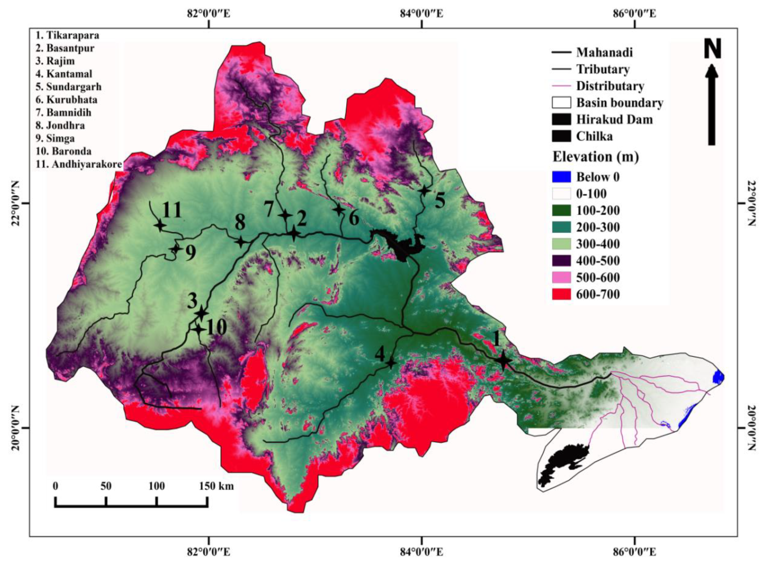
2. Study Area
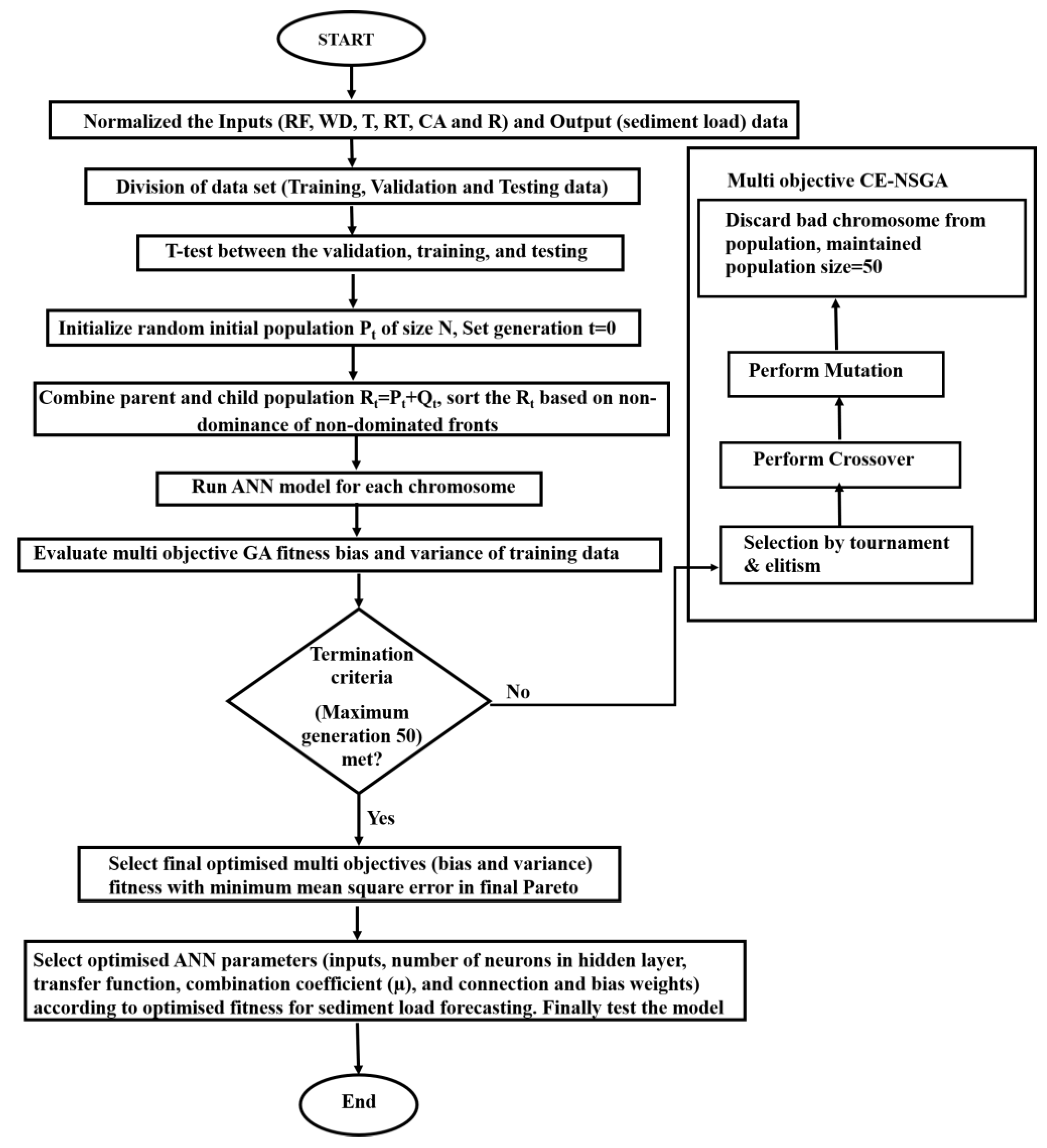
3. Methodology and Data
4. Results and Discussion
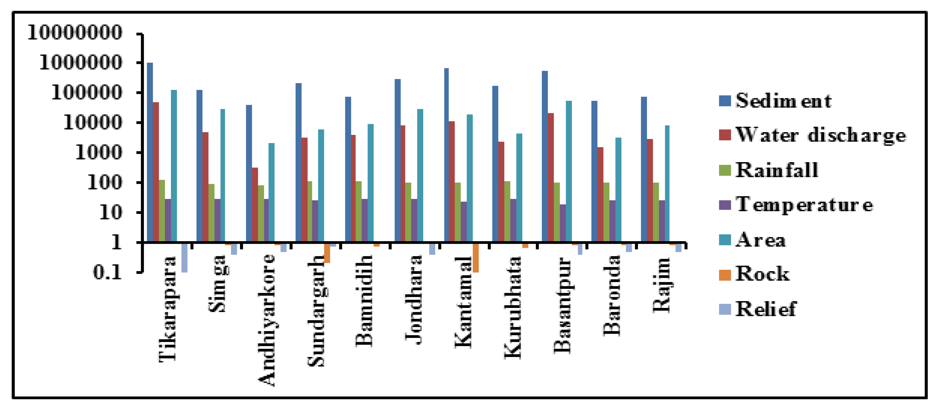
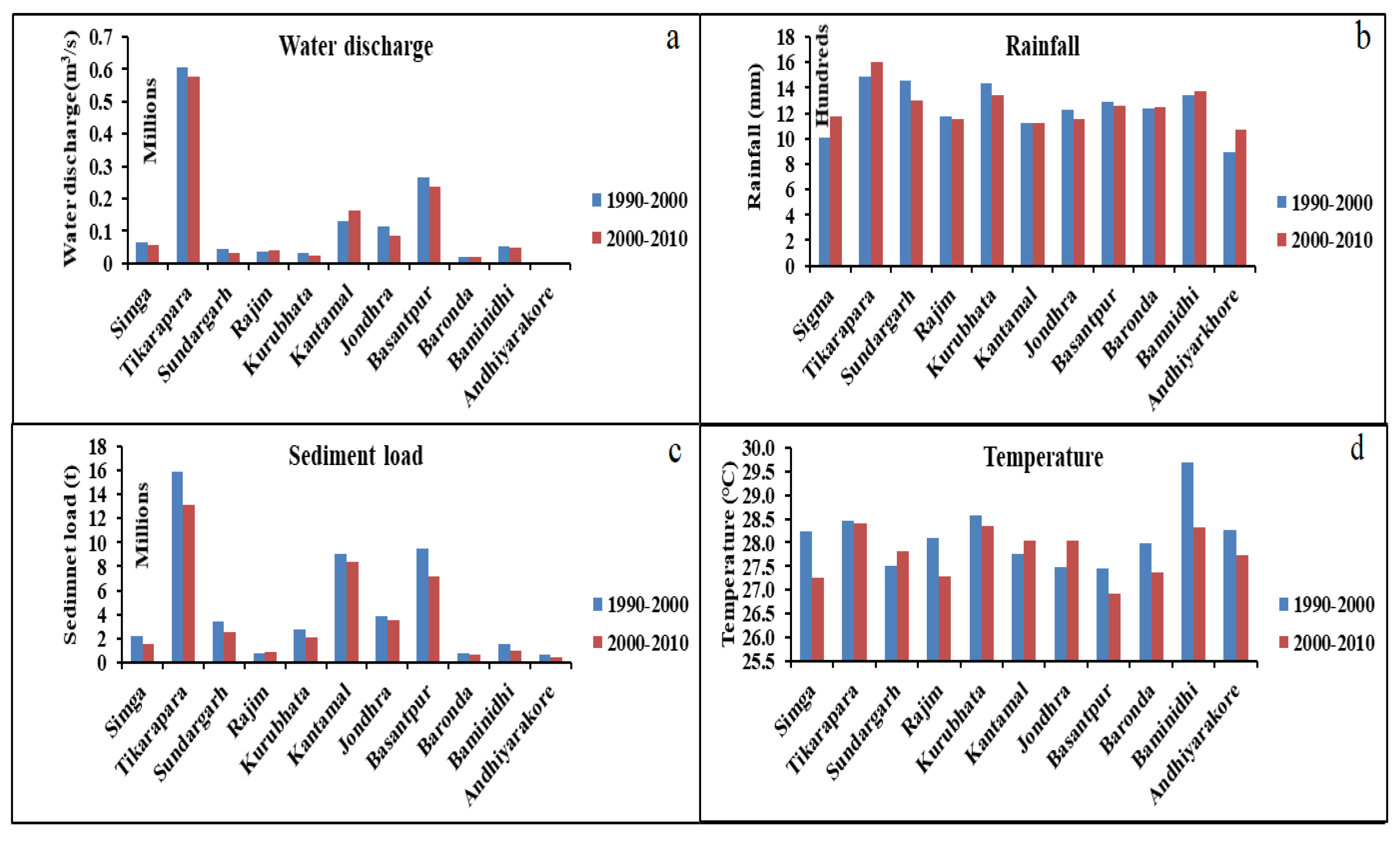
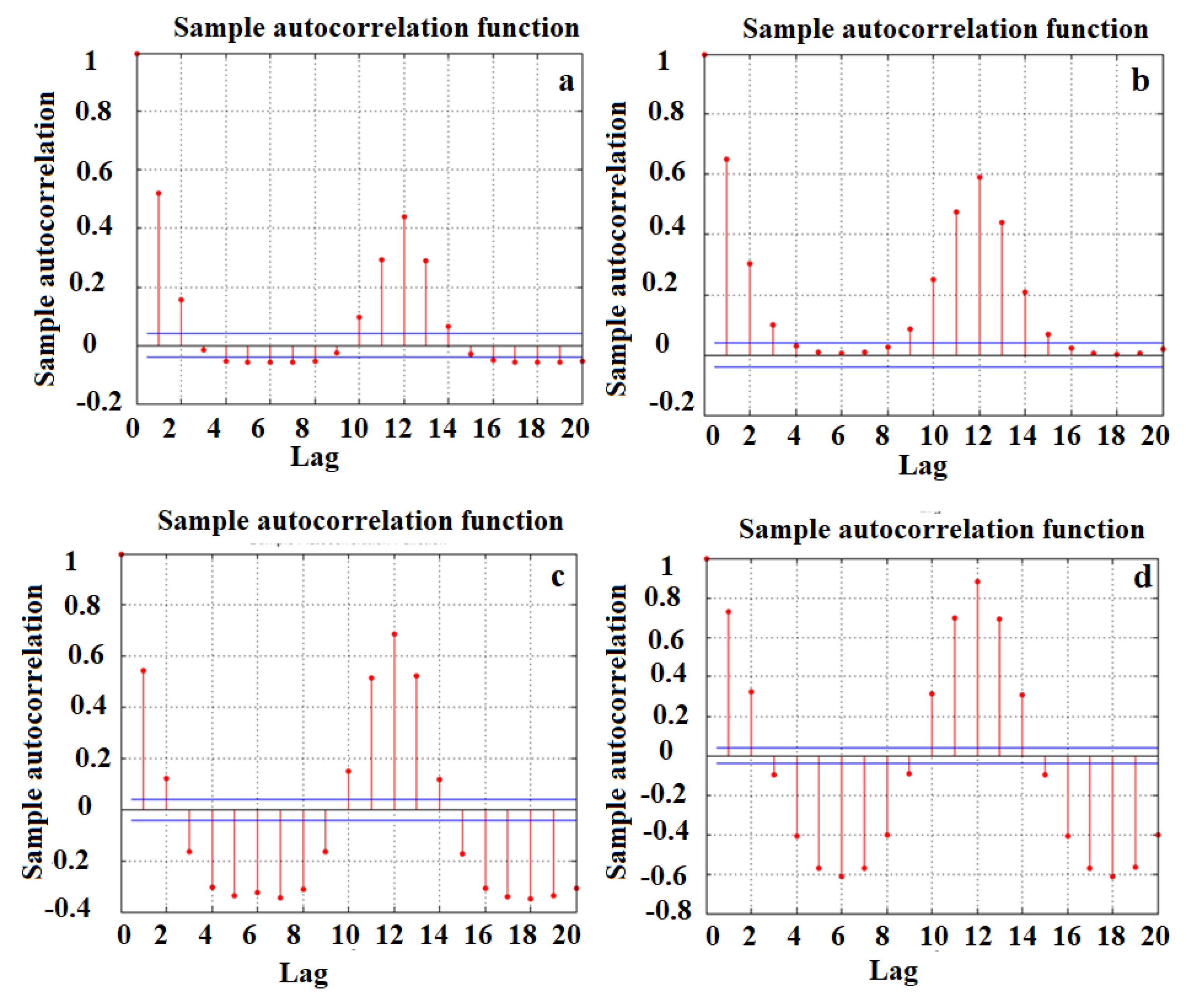
4.1. Data Analysis
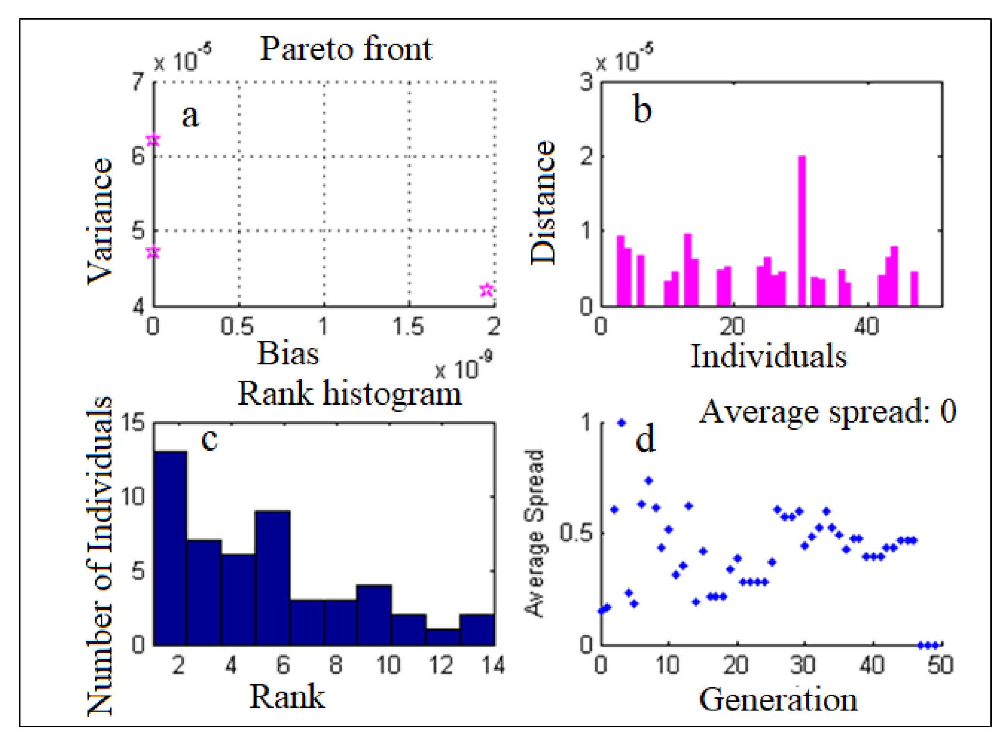
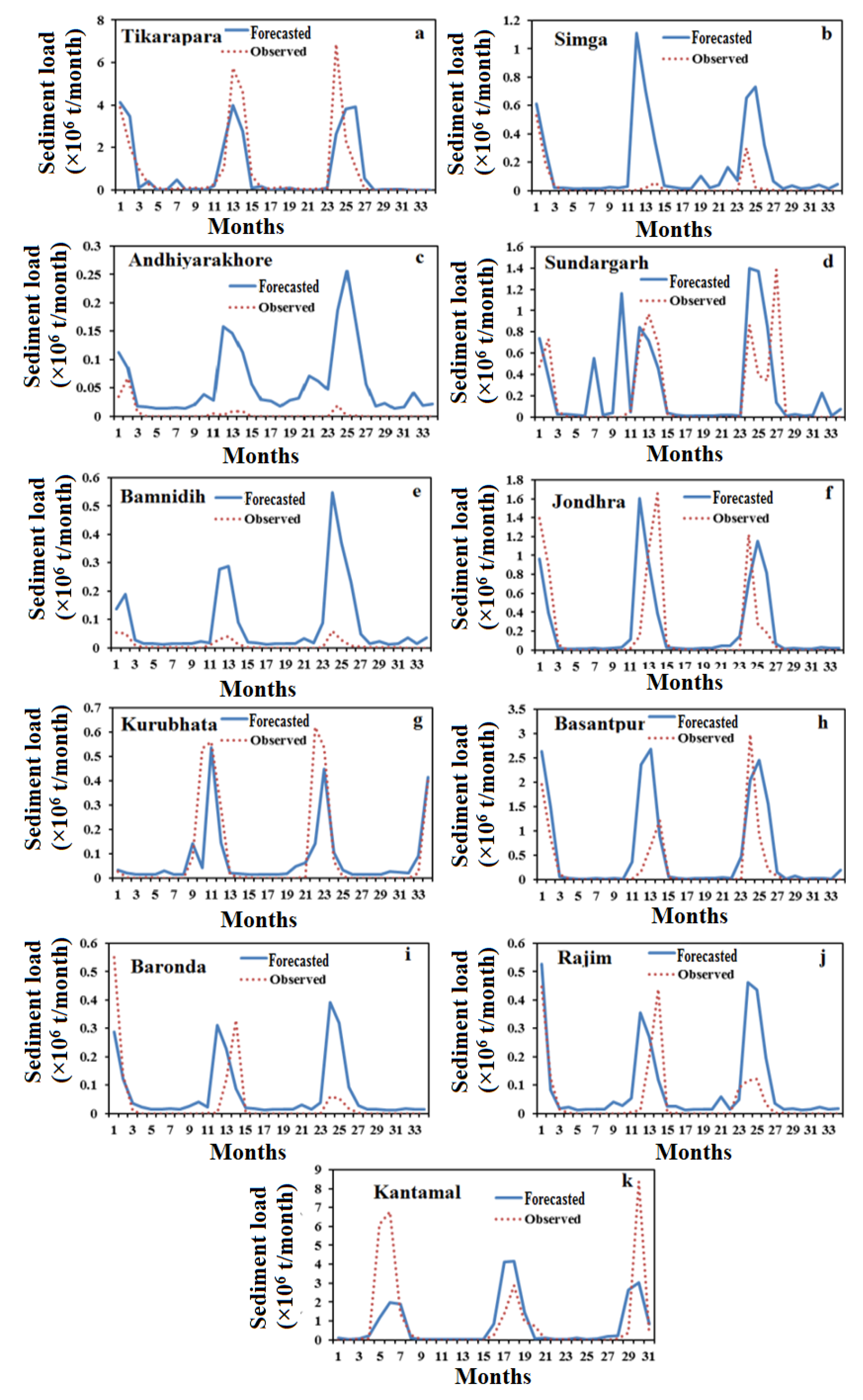
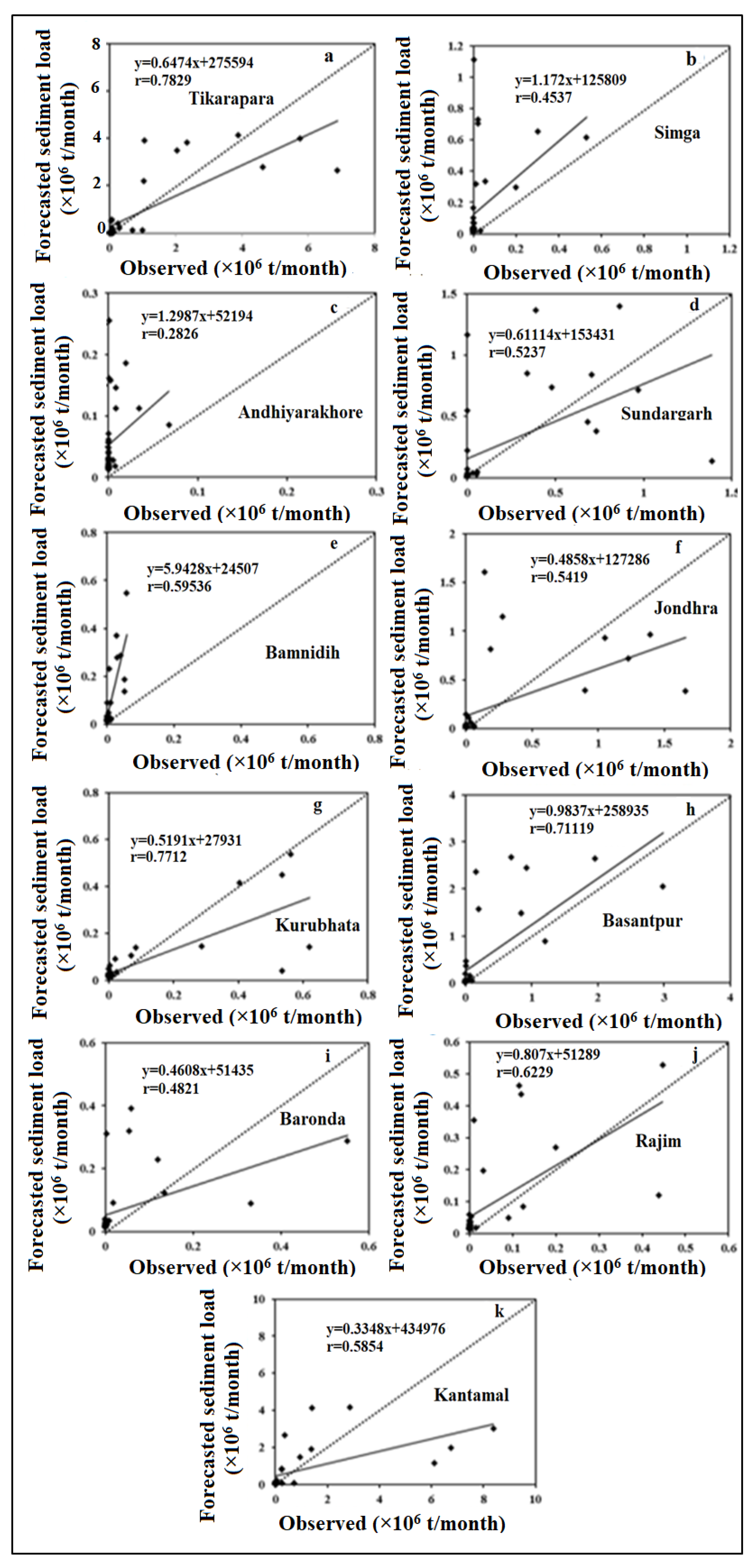
4.2. ANN-MOGA Forecasting Model
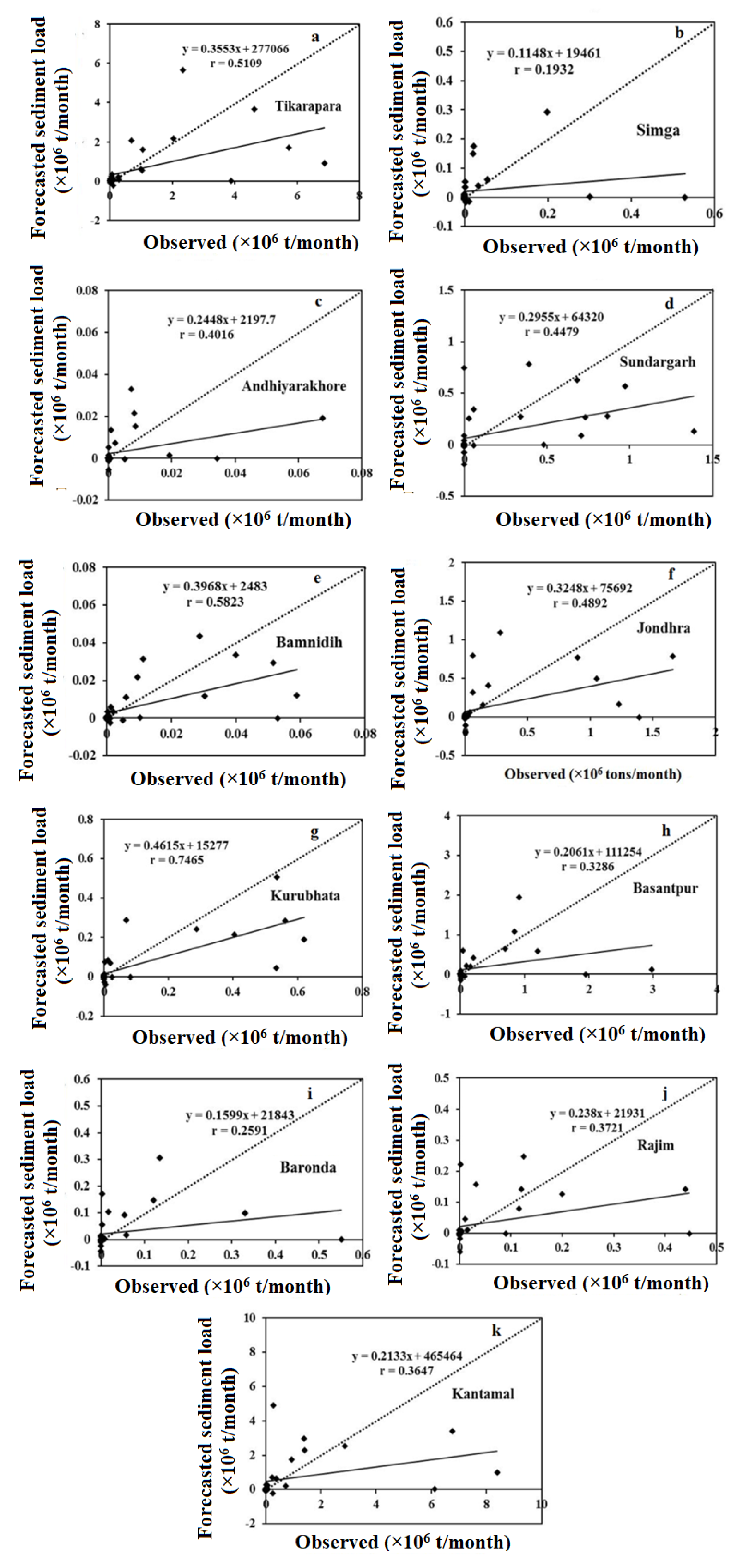
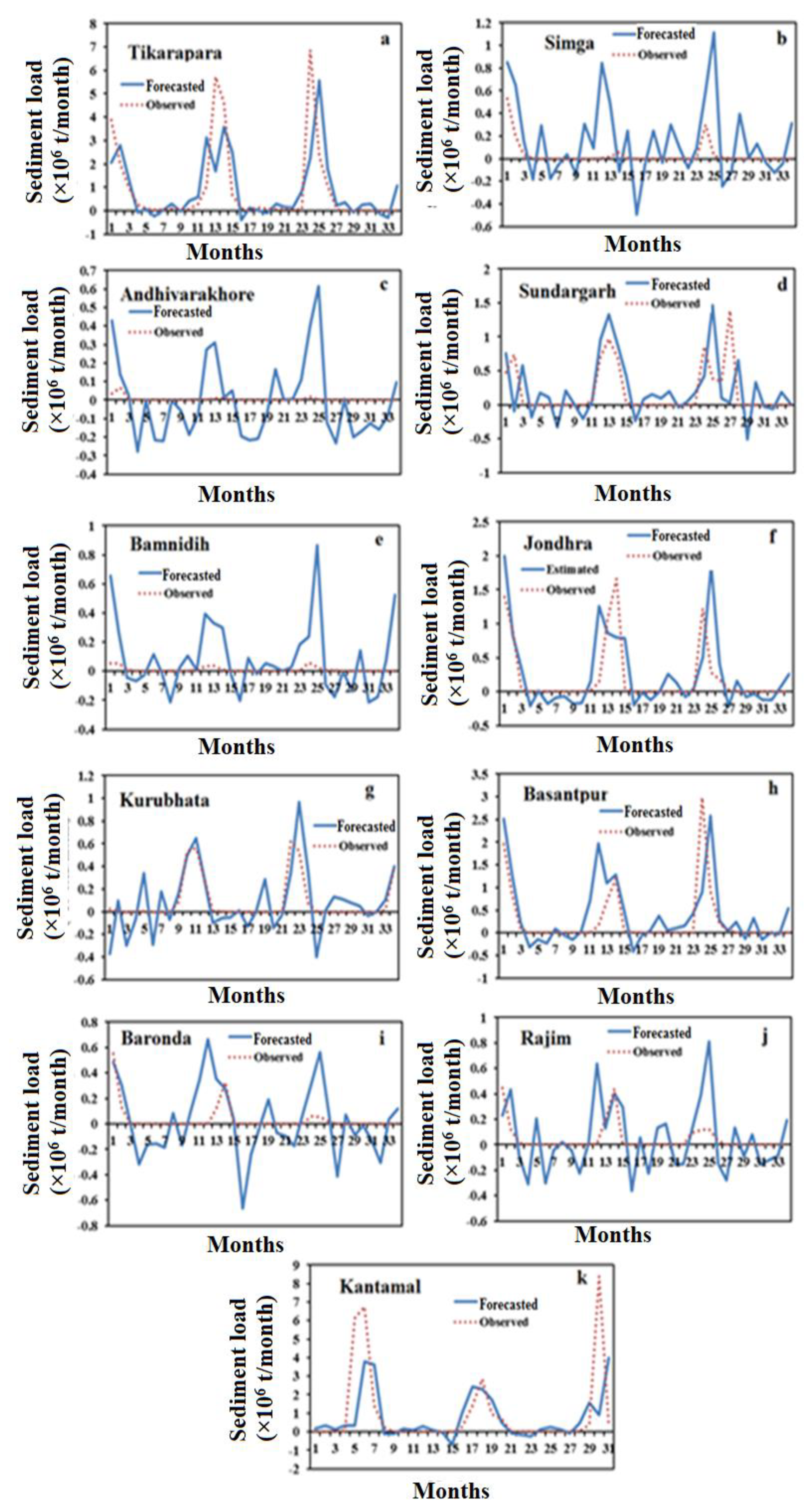
4.3. AR Forecasting Model
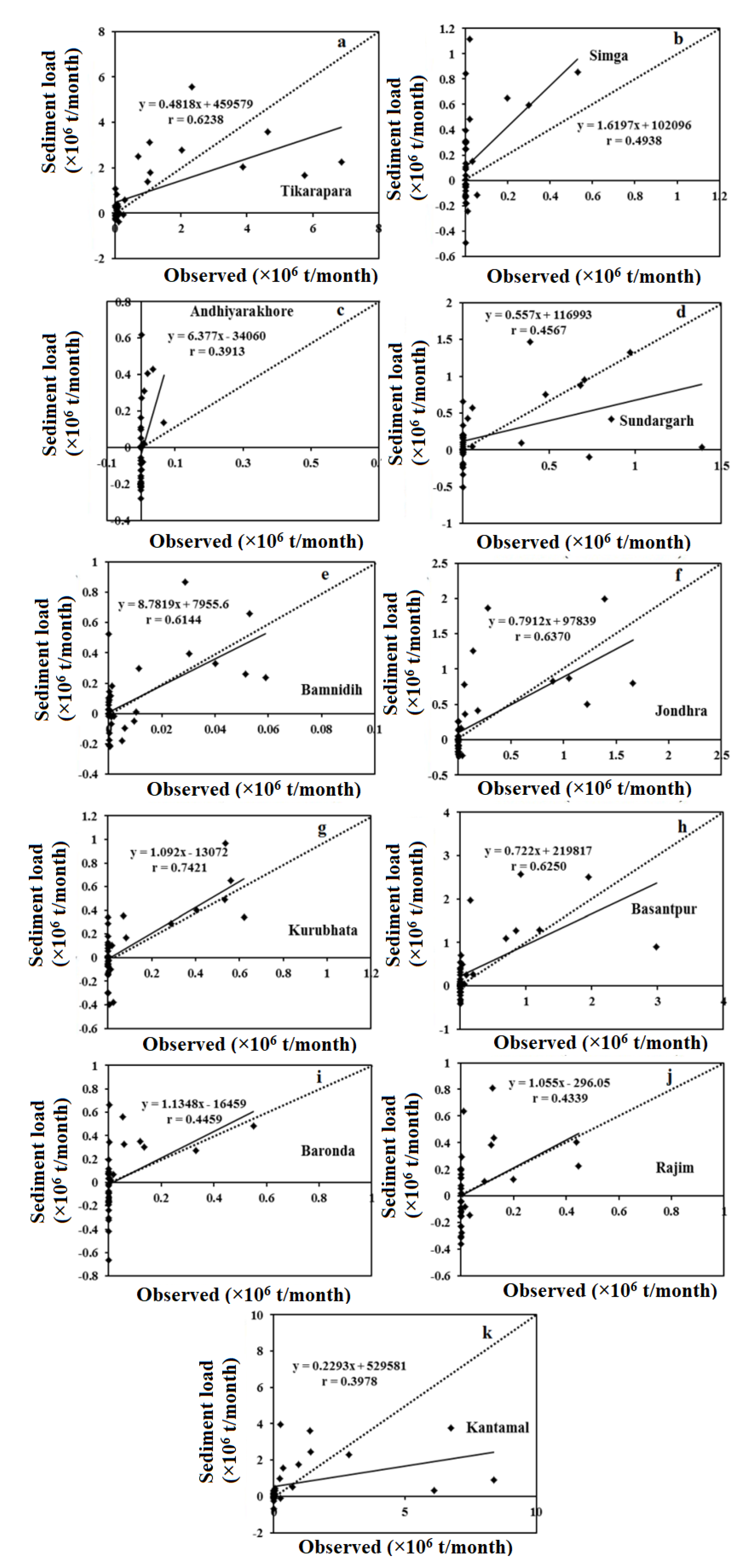
4.4. The Multivariate Autoregressive (MAR) Forecasting Model
4.5. Comparison Results of Forecasting Models
5. Conclusions
Author Contributions
Funding
Institutional Review Board Statement
Informed Consent Statement
Data Availability Statement
Conflicts of Interest
References
- Frémion, F.; Bordas, F.; Mourier, B.; Lenain, J.; Kestens, T.; Courtin-Nomade, A. Influence of dams on sediment continuity: A study case of a natural metallic contamination. Sci. Total Environ. 2016, 547, 282–294. [Google Scholar] [CrossRef] [PubMed]
- Xia, X.; Dong, J.; Wang, M.; Xie, H.; Xia, N.; Li, H.; Zhang, X.; Mou, X.; Wen, J.; Bao, Y. Effect of water-sediment regulation of the Xiaolangdi reservoir on the concentrations, characteristics, and fluxes of suspended sediment and organic carbon in the Yellow River. Sci. Total Environ. 2016, 571, 487–497. [Google Scholar] [CrossRef] [PubMed] [Green Version]
- Honorato, A.G.D.S.M.; Silva, G.B.L.D.; Guimarães Santos, C.A. Monthly streamflow forecasting using neuro-wavelet techniques and input analysis. Hydrol. Sci. J. 2018, 63, 2060–2075. [Google Scholar] [CrossRef] [Green Version]
- Dutta, S. Soil erosion, sediment yield and sedimentation of reservoir: A review. Model. Earth Syst. Environ. 2016, 2, 123. [Google Scholar] [CrossRef] [Green Version]
- Jansson, M.B. Land Erosion by Water in Different Climates; UNGI Report No. 57; Department of Physical Geography, University of Uppsala: Uppsala, Sweden, 1982. [Google Scholar]
- Syvitski, J.P.M.; Peckham, S.D.; Hilberman, R.; Mulder, T. Predicting the Terrestrial Flux of Sediment to the Global Ocean: A Planetary Perspective. Sediment. Geol. 2003, 162, 5–24. [Google Scholar] [CrossRef]
- Gupta, H.; Chakrapani, G.J. Temporal and spatial variations in water flow and sediment load in Narmada River Basin, India: Natural and man-made factors. Environ. Geol. 2005, 48, 579–589. [Google Scholar] [CrossRef]
- Ramesh, R.; Subramanian, V. Temporal, spatial and size variation in the sediment transport in the Krishna River basin, India. J. Hydrol. 1988, 98, 53–65. [Google Scholar] [CrossRef]
- Bastia, F.; Equeenuddin, S.M. Spatio-temporal variation of water flow and sediment discharge in the Mahanadi River, India. Glob. Planet. Chang. 2016, 144, 51–66. [Google Scholar] [CrossRef]
- Thodsen, H.; Hasholt, B.; Kjarsgaard, J.H. The influence of climate change on suspended sediment transport in Danish rivers. Hydrol. Process. 2008, 22, 764–774. [Google Scholar] [CrossRef]
- Merritt, W.S.; Letcher, R.A.; Jakeman, A.J. A review of erosion and sediment transport models. Environ. Model. Softw. 2003, 18, 761–799. [Google Scholar] [CrossRef]
- Salas, J.D.; Delleur, J.W.; Yevjevich, V.; Lane, W.L. Applied Modeling of Hydrologic Time Series; Water Resources Publications: Littleton, CO, USA, 1980; 484p. [Google Scholar]
- Adamowski, J.; Chan, H.F.; Prasher, S.O.; Ozga-Zielinski, B.; Sliusarieva, A. Comparison of multiple linear and nonlinear regression, autoregressive integrated moving average, artificial neural network, and wavelet artificial neural network methods for urban water demand forecasting in Montreal, Canada. Wat. Resour. Res. 2012, 48, W01528. [Google Scholar] [CrossRef]
- Pektas, A.O.; Cigizoglu, H.K. Long-range forecasting of suspended sediment. Hydrol. Sci. J. 2017, 62, 2415–2425. [Google Scholar] [CrossRef]
- Partal, T.; Cigizoglu, H.K. Estimation and forecasting of daily suspended sediment data using wavelet-neural networks. J. Hydrol. 2008, 358, 317–331. [Google Scholar] [CrossRef]
- Nourani, V.; Alizadeh, F.; Roushangar, K. Evaluation of a two-stage SVM and spatial statistics methods for modeling monthly river suspended sediment load. Water Resour. Manag. 2016, 30, 393–407. [Google Scholar] [CrossRef]
- Meshram, S.G.; Ghorbani, M.A.; Deo, R.C.; Kashani, M.H.; Meshram, C.; Karimi, V. New approach for sediment yield forecasting with a two-phase feedforward neuron network-particle swarm optimization model integrated with the gravitational search algorithm. Water Resour. Manag. 2019, 33, 2335–2356. [Google Scholar] [CrossRef]
- ASCE. Task Committee on Application of Artificial Neural Networks in Hydrology Artificial neural networks in hydrology. I: Preliminary concepts. J. Hydrol. Eng. 2000, 5, 115–123. [Google Scholar] [CrossRef]
- Reddy, P.V.B. Modelling and Optimization of Wire Electrical Discharge Machining of Cr-Mo-V Special Alloy Steel Using Neuro Genetic Approach. Ph.D. Thesis, Jawaharlal Nehru Technological University, Anantapur, India, 2014. [Google Scholar]
- Tokar, A.S.; Johnson, P.A. Rainfall-Runoff Modelling using Artificial Neural Networks. J. Hydrol. Eng. 1999, 4, 232–239. [Google Scholar] [CrossRef]
- Dawson, C.W.; Harpham, C.; Wilby, R.L.; Chen, Y. An evaluation of artificial neural network techniques for flow forecasting in the river Yangtze, China. Hydrol. Earth Syst. Sci. 2002, 6, 619–626. [Google Scholar] [CrossRef]
- Kar, A.K.; Lohani, A.K.; Goel, N.K.; Roy, G.P. Development of Flood Forecasting System Using Statistical and ANN Techniques in the Downstream Catchment of Mahanadi Basin, India. J. Water Resour. Prot. 2010, 2, 880–887. [Google Scholar]
- Bishop, M. Neural Networks for Pattern Recognition; Clarendon Press: Oxford, UK, 1998. [Google Scholar]
- Yadav, A.; Chatterjee, S.; Equeenuddin, S.M. Suspended Sediment Yield Estimation using Genetic Algorithm-based Artificial Intelligence Models in Mahanadi River. Hydrol. Sci. J. 2018, 63, 1162–1182. [Google Scholar] [CrossRef]
- Holland, J. Adaptation in Natural and Artificial Systems; The University of Michigan Press: Ann Arbor, MI, USA, 1975. [Google Scholar]
- Hosseini, S.A.; Abbaszadeh Shahri, A.; Asheghi, R. Prediction of bedload transport rate using a block combined network structure. Hydrol. Sci. J. 2022, 67, 117–128. [Google Scholar] [CrossRef]
- Chatterjee, S.; Bandopadhyay, S. Reliability estimation using a genetic algorithm-based artificial neural network: An application to a load-haul-dump machine. Expert Syst. Appl. 2012, 39, 10943–10951. [Google Scholar] [CrossRef]
- Asheghi, R.; Hosseini, S.A.; Saneie, M.; Shahri, A.A. Updating the neural network sediment load models using different sensitivity analysis methods: A regional application. J. Hydroinformatics 2020, 22, 562–577. [Google Scholar] [CrossRef] [Green Version]
- Adib, A.; Mahmoodi, A. Prediction of Suspended Sediment Load using ANN GA Conjunction Model with Markov Chain Approach at Flood Conditions. KSCE J. Civ. Eng. 2016, 1, 447–457. [Google Scholar] [CrossRef]
- Chatterjee, S.; Bandopadhyay, S. Goodnews Bay Platinum Resource Estimation Using Least Squares Support Vector Regression with Selection of Input Space Dimension and Hyperparameters. Nat. Resour. Res. 2016, 20, 117–129. [Google Scholar] [CrossRef]
- Samarasinghe, S. Neural Networks for Applied Sciences and Engineering: From Fundamentals to Complex Pattern Recognition; CRC Press: Boca Raton, FL, USA, 2016; p. 555. [Google Scholar]
- Geman, S.; Bienenstock, E.; Doursat, R. Neural networks and the bias/variance dilemma. Neural Comput. 1992, 4, 1–58. [Google Scholar] [CrossRef]
- Rosales-Perez, A.; Escalante, H.J.; Gonzalez, J.A.; Reyes-Garcia, C.A. Bias and variance optimization for SVMs model selection. In Proceedings of the Twenty-Sixth International FLAIRS Conference, St. Pete Beach, FL, USA, 22–24 May 2013. [Google Scholar]
- Kulasiri, D.; Verwoerd, V. Stochastic Dynamics: Modeling Solute Transport in Porous Media; North Holland Series in Applied Mathematics and Mechanics; Elsevier: Amsterdam, The Netherlands, 2002; p. 44. [Google Scholar]
- Levin, S.A. Population dynamics in models in heterogeneous environments. Annu. Rev. Ecol. Syst. 1976, 7, 287. [Google Scholar] [CrossRef]
- Deb, K.; Pratap, A.; Agarwal, S.; Meyarivan, T. A fast and elitist multi-objective genetic algorithm: NSGA-II. IEEE Trans. Evol. Comput. 2002, 6, 181–197. [Google Scholar] [CrossRef] [Green Version]
- Bharti, P.S.; Maheshwari, S.; Sharma, C. Multi-objective optimization of electric-discharge machining process using controlled elitist NSGA-II. J. Mech. Sci. Technol. 2012, 26, 1875–1883. [Google Scholar] [CrossRef]
- Behzadian, K.; Kapelan, Z.; Savic, D.; Ardeshir, A. Stochastic sampling design using multi-objective genetic algorithm and adaptive neural network. Environ. Model. Softw. 2009, 24, 530–541. [Google Scholar] [CrossRef] [Green Version]
- Zhou, C.C.; Yin, G.F.; Hu, X.B. Multi-objective optimization of material selection for sustainable products: Artificial neural networks and genetic algorithm approach. Mater. Des. 2009, 30, 1209–1215. [Google Scholar] [CrossRef]
- Yadav, A.; Chatterjee, S.; Equeenuddin, S.M. Suspended sediment yield modeling in Mahanadi River, India by multi-objective optimization hybridizing artificial intelligence algorithms. Int. J. Sediment Res. 2021, 36, 76–91. [Google Scholar] [CrossRef]
- Sakai, K.; Osawa, K.; Yoshinaga, A. Development of suspended sediment concentration analysis model and its application with multi-objective optimization. Paddy Water Environ. 2005, 3, 201–209. [Google Scholar] [CrossRef]
- Peng, Y.; Ji, C.; Gu, R. Multiobjective optimization model for coordinatec regulation of water flow and sediment in cascade reservoirs. Water Resour. Manag. 2014, 28, 4019–4033. [Google Scholar] [CrossRef]
- Cigizoglu, H.K.; Kisi, O. Methods to improve the neural network performance in suspended sediment estimation. J. Hydrol. 2006, 317, 221–238. [Google Scholar] [CrossRef]
- Cigizoglu, H.K.; Alp, M. Generalized regression neural network in modelling river sediment yield. Adv. Eng. Softw. 2006, 37, 63–68. [Google Scholar] [CrossRef]
- Piotrowski, A.P.; Napiorkowski, M.J.; Napiorkowski, J.J.; Osuch, M. Comparing various artificial neural network types for water temperature prediction in rivers. J. Hydrol. 2015, 529, 302–315. [Google Scholar] [CrossRef]
- Kant, A.; Suman, P.K.; Giri, B.K.; Tiwari, M.K.; Chatterjee, C.; Nayak, P.C.; Kumar, S. Comparison of multi-objective evolutionary neural network, adaptive neuro-inference system and bootstrap-based neural network for flood forecasting. Neural Comput. Appl. 2013, 23, S231–S246. [Google Scholar] [CrossRef]
- India-WRIS. Water Resources Information System of India. Available online: http://india-wris.nrsc.gov.in/wrpinfo/index.php?title=Mahanadi (accessed on 8 August 2016).
- Yadav, A.; Chatterjee, S.; Equeenuddin, S.M. Prediction of Suspended Sediment Yield by Artificial Neural Network and Traditional Mathematical Model in Mahanadi River Basin, India. J. Sustain. Water Resour. Manag. 2017, 4, 745–759. [Google Scholar] [CrossRef]
- Rojas, R. Neural Network: A Systematic Introduction; Springer: Berlin, Germany, 1996; pp. 151–184. [Google Scholar]
- Hagan, M.T.; Menhaj, M.B. Training feedforward networks with the Marquardt algorithm. IEEE Trans. Neural Netw. 1994, 5, 989–993. [Google Scholar] [CrossRef]
- Ebtehaj, I.; Bonakdari, H.; Safari, M.J.S.; Gharabaghi, B.; Zaji, A.H.; Madavar, H.R.; Khozani, Z.S.; Es-haghi, M.S.; Shishegaran, A.; Mehr, A.D. Combination of sensitivity and uncertainty analyses for sediment transport modeling in sewer pipes. Int. J. Sediment Res. 2020, 35, 157–170. [Google Scholar] [CrossRef]
- Riahi-Madvar, H.; Gharabaghi, B. Pre-processing and Input Vector Selection Techniques in Computational Soft Computing Models of Water Engineering. In Computational Intelligence for Water and Environmental Sciences; Springer: Singapore, 2022; pp. 429–447. [Google Scholar]
- Dehghani, M.; Seifi, A.; Riahi-Madvar, H. Novel forecasting models for immediate-short-term to long-term influent flow prediction by combining ANFIS and grey wolf optimization. J. Hydrol. 2019, 576, 698–725. [Google Scholar] [CrossRef]
- Riahi-Madvar, H.; Dehghani, M.; Memarzadeh, R.; Gharabaghi, B. Short to long-term forecasting of river flows by heuristic optimization algorithms hybridized with ANFIS. Water Resour. Manag. 2021, 35, 1149–1166. [Google Scholar] [CrossRef]
- Riahi-Madvar, H.; Seifi, A. Uncertainty analysis in bed load transport prediction of gravel-bed rivers by ANN and ANFIS. Arab. J. Geosci. 2018, 11, 1–20. [Google Scholar] [CrossRef]
- Gowda, C.C.; Mayya, S.G. Comparison of back propagation neural network and genetic algorithm neural network for stream flow prediction. J. Comput. Environ. Sci. 2014, 290127. [Google Scholar] [CrossRef] [Green Version]
- Senthil Kumar, A.R.; Sudheer, K.P.; Jain, S.K.; Agarwal, P.K. Rainfall-runoff modelling using artificial neural networks: Comparison of network types. Hydrol. Process. Int. J. 2005, 19, 1277–1291. [Google Scholar] [CrossRef]
- Ghosh, A.; Das, M.K. Non-dominated rank-based sorting genetic algorithms. Fundam. Inform. 2008, 83, 231–252. [Google Scholar]
- Moriasi, D.N.; Arnold, J.G.; Van Liew, M.W.; Bingner, R.L.; Harmel, R.D.; Veith, T.L. Model Evaluation Guidelines for Systematic Quantification of Accuracy in Watershed Simulations. Trans. ASABE 2007, 50, 885–900. [Google Scholar] [CrossRef]


| Stations | r1 (WD-SL) | r2 (SL-RF) | r3 (SL-T) |
|---|---|---|---|
| Tikarapara | 0.891951579 | 0.667566099 | 0.167164223 |
| Sundargarh | 0.933162643 | 0.719490012 | 0.083275757 |
| Simga | 0.912171157 | 0.669144968 | 0.016117111 |
| Jondhara | 0.953615062 | 0.634788084 | 0.024002708 |
| Andhiyarakhore | 0.930440984 | 0.679483679 | 0.172300271 |
| Kurubhata | 0.914790531 | 0.739541786 | 0.09457768 |
| Bamnidih | 0.792975574 | 0.673800075 | 0.19294038 |
| Rajim | 0.933515452 | 0.652771319 | −0.053703323 |
| Kantamal | 0.784858255 | 0.653582343 | 0.045884228 |
| Baronda | 0.896128553 | 0.718865603 | 0.170015607 |
| Basantpur | 0.900261237 | 0.717722236 | 0.120971863 |
| Models | Number of Initial Inputs | Input Parameters |
|---|---|---|
| ANN-MOGA-51 | 51 | SL, WD, RF, T, RT, R and CA |
| ANN-MOGA-48 | 48 | SL, WD, RF and T |
| ANN-MOGA-15 | 15 | SL, RT, R and CA |
| ANN-MOGA-12 | 12 | SL |
| Models | RMSE | Initially Inputs No. | MSE | MAE | VAR | r |
|---|---|---|---|---|---|---|
| ANN-MOGA-51 | 0.011639 | 51 | 0.000135 | 0.003802 | 0.000136 | 0.643313 |
| ANN-MOGA-48 | 0.013343 | 48 | 0.000178 | 0.00381194 | 0.0001783 | 0.5674853 |
| ANN-MOGA-15 | 0.013637 | 15 | 0.000186 | 0.0044 | 0.000186 | 0.513217 |
| ANN-MOGA-12 | 0.01181 | 12 | 0.000139 | 0.003626 | 0.00014 | 0.623344 |
| Models | Transfer Function | Neurons | Inputs | µ |
|---|---|---|---|---|
| ANN-MOGA-51 | Log-sigmoid, pure linear | 29 | 22 | 2 |
| ANN-MOGA-48 | Tan-sigmoid, pure linear | 19 | 21 | 9 |
| ANN-MOGA-15 | Pure linear, tan-sigmoid | 15 | 10 | 10 |
| ANN-MOGA-12 | Tan-sigmoid, pure linear | 4 | 6 | 6 |
| ANN-MOGA-51 | MSE | RMSE | r | Error Variance | MAE |
|---|---|---|---|---|---|
| Training | 0.000241 | 0.015526 | 0.668938 | 0.000241 | 0.004677 |
| Validation | 5.25 × 10⁻⁵ | 0.007243 | 0.7730 | 5.26 × 10⁻⁵ | 0.002867 |
| Testing | 0.000135 | 0.011639 | 0.643313 | 0.000136 | 0.003802 |
| Tikarapara | 0.000396 | 0.019905 | 0.731051 | 0.000407 | 0.010517 |
| Simga | 1.17 × 10⁻⁵ | 0.003422 | 0.5930 | 9.81 × 10⁻⁶ | 0.001707 |
| Andhiyarakhore | 1.10 × 10⁻⁵ | 0.003319 | 0.4001 | 9.06 × 10⁻⁵ | 0.001749 |
| Sundargarh | 2.60 × 10⁻⁵ | 0.005097 | 0.635 | 2.67 × 10⁻⁵ | 0.002466 |
| Bamnidih | 3.33 × 10⁻⁵ | 0.005769 | 0.695 | 3.27 × 10⁻⁵ | 0.002765 |
| Jondhara | 3.02 × 10⁻⁵ | 0.005499 | 0.737 | 2.91 × 10⁻⁵ | 0.002534 |
| Kurubhata | 2.06 × 10⁻⁵ | 0.001434 | 0.914 | 1.97 × 10⁻⁶ | 0.000865 |
| Basantpur | 0.000229 | 0.015121 | 0.478143 | 0.000222 | 0.006185 |
| Baronda | 5.66 × 10⁻⁶ | 0.002379 | 0.495 | 5.23 × 10⁻⁶ | 0.001319 |
| Rajim | 2.10 × 10⁻⁶ | 0.001448 | 0.669 | 2.15 × 10⁻⁶ | 0.000722 |
| Kantamal | 0.000806 | 0.028395 | 0.659518 | 0.000801 | 0.01198 |
| AR | RMSE | MSE | MAE | VAR | r |
|---|---|---|---|---|---|
| Training | 0.01640 | 0.00027 | 0.00473 | 0.00027 | 0.61268 |
| Testing | 0.01335 | 0.00018 | 0.00365 | 0.00018 | 0.49670 |
| Tikarapara | 0.02576 | 0.00066 | 0.01119 | 0.00066 | 0.51087 |
| Simga | 0.00185 | 3.42 × 10⁻⁶ | 0.00069 | 3.49 × 10−06 | 0.19322 |
| Andhiyarakhore | 0.00020 | 4.07 × 10⁻⁸ | 9.30×10⁻⁵ | 4.15 × 10−08 | 0.40166 |
| Sundargarh | 0.00555 | 3.08 × 10⁻⁵ | 0.00303 | 3.02 × 10−05 | 0.44791 |
| Bamnidih | 0.00024 | 5.56 × 10⁻⁸ | 0.00012 | 5.46 × 10−08 | 0.58226 |
| Jondhara | 0.00668 | 4.46 × 10⁻⁵ | 0.00323 | 4.48 × 10−05 | 0.48917 |
| Kurubhata | 0.00222 | 4.92 × 10⁻⁶ | 0.00103 | 4.72 × 10−06 | 0.74650 |
| Basantpur | 0.01059 | 0.00011 | 0.00411 | 0.00011 | 0.32857 |
| Baronda | 0.00187 | 3.49 × 10⁻⁶ | 0.00073 | 3.56 × 10⁻⁶ | 0.25906 |
| Rajim | 0.00177 | 3.14 × 10⁻⁶ | 0.00079 | 3.18 × 10⁻⁶ | 0.37205 |
| Kantamal | 0.03386 | 0.00115 | 0.01481 | 0.00116 | 0.36473 |
| MAR | MAE | VAR | r | MSE | RMSE |
|---|---|---|---|---|---|
| Training | 0.00640 | 0.00023 | 0.68010 | 0.00023 | 0.01516 |
| Testing | 0.00562 | 0.00017 | 0.55620 | 0.00017 | 0.01296 |
| Tikarapara | 0.01306 | 0.00054 | 0.62380 | 0.00052 | 0.02284 |
| Simga | 0.00395 | 2.65×10⁻⁵ | 0.49380 | 2.99×10⁻⁵ | 0.00547 |
| Andhiyarakhore | 0.00260 | 1.20×10⁻⁵ | 0.39130 | 1.16×10⁻⁵ | 0.00341 |
| Sundargarh | 0.00486 | 4.91×10⁻⁵ | 0.45670 | 4.79×10⁻⁵ | 0.00692 |
| Bamnidih | 0.00272 | 1.53×10⁻⁵ | 0.61440 | 1.66×10⁻⁵ | 0.00407 |
| Jondhara | 0.00458 | 5.44×10⁻⁵ | 0.63700 | 5.36×10⁻⁵ | 0.00732 |
| Kurubhata | 0.00228 | 1.01×10⁻⁵ | 0.74210 | 9.80×10⁻⁶ | 0.00313 |
| Basantpur | 0.00610 | 0.00010 | 0.62500 | 0.00011 | 0.01025 |
| Baronda | 0.00306 | 1.75×10⁻⁵ | 0.44590 | 1.70×10⁻⁵ | 0.00412 |
| Rajim | 0.00309 | 1.64×10⁻⁵ | 0.43390 | 1.59×10⁻⁵ | 0.00398 |
| Kantamal | 0.01652 | 0.00111 | 0.39780 | 0.00108 | 0.03292 |
| Models | ANN-MOGA-51 | MAR | AR | |||
|---|---|---|---|---|---|---|
| Statistics | RMSE | r | RMSE | r | RMSE | r |
| Testing | 0.01164 | 0.6433 | 0.01296 | 0.5562 | 0.01335 | 0.4967 |
| Tikarapara | 0.01991 | 0.7311 | 0.02284 | 0.6238 | 0.02576 | 0.5109 |
| Simga | 0.00342 | 0.5930 | 0.00547 | 0.4938 | 0.00185 | 0.1932 |
| Andhiyarakhore | 0.00332 | 0.4001 | 0.00341 | 0.3913 | 0.00020 | 0.4017 |
| Sundargarh | 0.00510 | 0.6350 | 0.00692 | 0.4567 | 0.00555 | 0.4479 |
| Bamnidih | 0.00577 | 0.6950 | 0.00407 | 0.6144 | 0.00024 | 0.5821 |
| Jondhara | 0.00550 | 0.7370 | 0.00732 | 0.6370 | 0.00668 | 0.4892 |
| Kurubhata | 0.00143 | 0.9140 | 0.00313 | 0.7421 | 0.00222 | 0.7465 |
| Basantpur | 0.01512 | 0.4781 | 0.01025 | 0.6250 | 0.01059 | 0.3286 |
| Baronda | 0.00238 | 0.4950 | 0.00412 | 0.4459 | 0.00187 | 0.2591 |
| Rajim | 0.00145 | 0.6690 | 0.00398 | 0.4339 | 0.00177 | 0.3721 |
| Kantamal | 0.02840 | 0.6595 | 0.03292 | 0.3978 | 0.03386 | 0.3647 |
Disclaimer/Publisher’s Note: The statements, opinions and data contained in all publications are solely those of the individual author(s) and contributor(s) and not of MDPI and/or the editor(s). MDPI and/or the editor(s) disclaim responsibility for any injury to people or property resulting from any ideas, methods, instructions or products referred to in the content. |
© 2023 by the authors. Licensee MDPI, Basel, Switzerland. This article is an open access article distributed under the terms and conditions of the Creative Commons Attribution (CC BY) license (https://creativecommons.org/licenses/by/4.0/).
Share and Cite
Yadav, A.; Ali Albahar, M.; Chithaluru, P.; Singh, A.; Alammari, A.; Kumar, G.V.; Miro, Y. Hybridizing Artificial Intelligence Algorithms for Forecasting of Sediment Load with Multi-Objective Optimization. Water 2023, 15, 522. https://doi.org/10.3390/w15030522
Yadav A, Ali Albahar M, Chithaluru P, Singh A, Alammari A, Kumar GV, Miro Y. Hybridizing Artificial Intelligence Algorithms for Forecasting of Sediment Load with Multi-Objective Optimization. Water. 2023; 15(3):522. https://doi.org/10.3390/w15030522
Chicago/Turabian StyleYadav, Arvind, Marwan Ali Albahar, Premkumar Chithaluru, Aman Singh, Abdullah Alammari, Gogulamudi Vijay Kumar, and Yini Miro. 2023. "Hybridizing Artificial Intelligence Algorithms for Forecasting of Sediment Load with Multi-Objective Optimization" Water 15, no. 3: 522. https://doi.org/10.3390/w15030522