
Analysis of the Effects of Reservoir Operating Scenarios on Downstream Flood Damage Risk Using an Integrated Monte Carlo Modelling Approach


1
Department of Engineering, University of Messina, 98166 Messina, Italy
2
Department of Engineering, University of Palermo, 90138 Palermo, Italy
*
Author to whom correspondence should be addressed.
Water 2023, 15(3), 550; https://doi.org/10.3390/w15030550
Submission received: 15 December 2022
/
Revised: 19 January 2023
/
Accepted: 27 January 2023
/
Published: 30 January 2023
(This article belongs to the Section Water Resources Management, Policy and Governance)
Abstract
:The aim of this study is to analyse the effects of reservoir operating scenarios, for flood damage evaluation downstream of a dam, using a Monte Carlo bivariate modelling chain. The proposed methodology involves a stochastic procedure to calculate flood hydrographs and the evaluation of the consequent flood inundation area by applying a 2D hydraulic model. These results are used to estimate the inundation risk and, as consequence, the relative damage evaluation under different water level conditions in an upstream reservoir. The modelling chain can be summarized as follows: single synthetic stochastic rainfall event generation by using a Monte Carlo procedure through a bivariate copulas analysis; synthetic bivariate stochastic inflow hydrograph derivation by using a conceptual fully distributed model starting from synthetic hyetographs above the derived; flood hydrographs routing through the reservoir taking in an account of the initial level in the reservoir; flood inundation mapping by applying a 2D hydraulic simulation and damage evaluation through the use of appropriate depth-damage curves. This allowed for the evaluation of the influence of initial water level on flood risk scenarios. The procedure was applied to the case study of the floodplain downstream from the Castello reservoir, within the Magazzolo river catchment, located in the southwestern part of Sicily (Italy).
1. Introduction
Floods are an environmental hazard that can cause heavy economic, environmental, and social losses. Therefore, their control is an important issue for damage mitigation worldwide. Floodwater storage construction facilities, such as reservoir dams, are some of the most common strategies of flood control through structural measures, which can also provide other benefits to people or local economies, including water supply during dry season, irrigation, recreation, and hydroelectric power [1,2,3].
However, large populations, infrastructures, and properties are located downstream of a dam, and in case of its failure or break, this can pose significant risks. When dams fail or malfunction, they can adversely affect people, their livelihoods, jobs, and businesses. Between 2000 and 2009, more than 200 dam breaks or failures occurred in many countries, causing disastrous effects on downstream areas [4].
Due to climate change and increased urban development, consequences of dam reservoir incorrect operational management have become much higher in the last decades [5,6]. Hence, a correct risk and damage assessment evaluation needs to consider all artificial structures holding water, which represent potential sources of flooding during operational flood control and in the case of possible failure of the structure.
Dam risk management and mitigation has become a high priority of organizations concerned with dams and valley safety, as well as with civil protection procedures. Most of the potential damages and losses occur along the downstream valleys. Past events show this evidence [7], and recent dam safety legislation includes some procedures related to the downstream effects of a dam failure. An effective mitigation of possible hazards, due to a dam accident or incident, clearly imposes an integrated risk management, including both the dam risk control and the valley protection. European Flood Directive 2007/60 requires potential damage evaluation to estimate the magnitude of the consequences of a flood.
In Italy, national laws and several technical guidelines have highlighted the need to set up specific operational dam reservoir management rules in case of downstream flooding risk by preparing appropriate reservoir flood control operation plans [8,9]. Currently, the evaluation and technical approval of projects related to dams is carried out by the National Dams Authority. The current Dam Regulation, relevant not only to the design and construction of new dams and to design of rehabilitation works of existing dams but also to the emergency action management in case of extreme events, is divided into two parts. The first one deals with the formal and administrative procedures, as well as general technical aspects to be followed. The second part is, instead, the “Technical Rules” defining all the technical details to be considered in the dam design and functionality. Emergency Action Plans (EAP) must be set up by local Civil Protection Authorities and coordinated by the Prefecture for various types of risks, especially for the downstream hydraulic risks of the dam. The Technical Rules are, in fact, aimed to ensure that, in case of extreme events, dams assure their operative functionality during the emergency phase. The Directive also establishes updated conditions to activate alert phases for dam safety and management of downstream hydraulic risks, defining the actions to be implemented in these phases.
Estimation of the potential damage, associated with the release of water downstream of a dam if an extreme event occurs, is a fundamental exercise to make decisions in ensuring safety of the properties placed downstream that, in case of flooding, must be reimbursed.
For calculating the potential damage of the properties for a forecasted or measured flood event, obtaining information about areas that would be inundated is a must and could be useful to the decision maker, in real time, to offer flexibility for adapting the water level in the dam to changing realities. Scientific literature emphasizes the importance of the reservoir operation optimization, finalized to define correct release decisions that guarantee not only the more common objectives of water management, such as the hydropower production, a reliable water supply, etc. [5,10,11,12], but the mitigation of downstream flood as well [13,14,15,16].
The inundated area in downstream areas depends on various factors, such as the height of the dam, its initial water level (IWL), the nature of failure, and the downstream vulnerability. The inundation maps show the areas that are likely to be submerged for different flood hydrographs as a function of the above factors.
When flooding occurs in a medium–big catchment, it is possible to carry out a two-dimensional analysis by running a model, in real time, in a reasonable amount of time to make appropriate decisions. However, in case of flash flooding, the time between the forecasting and the consequent flooding is not enough; hence, the a priori knowledge of the damage associated with a forecasted or measured flood event can be a valid approach.
Data availability is the main problem in flood hydrograph estimation. Even if discharge data are available, the length of the available hydrological series can be too short for any hydrological evaluation. In these cases, flood events may be estimated via rainfall-runoff simulation using observed precipitation data or generated data through stochastic simulation methods as the input. In this latter case, Monte Carlo simulation methods can be used to generate long series of rainfall events defined by their duration, volume, and temporal and spatial storm distribution [17,18,19,20,21].
Moreover, since flood peaks and corresponding flood volumes are variables of the same phenomenon, they should be correlated and, consequently, bivariate statistical analyses, and the theory of the Copula in particular, should be applied [19,20,21,22,23]. In literature, many hydrological applications (i.e., floods, storms, droughts), with bivariate flood frequency analysis by using copulas, are already presented and implemented in many case studies [20,21,22,23,24,25,26,27].
Dam hydrological safety assessment can, hence, be improved by bivariate flood frequency analysis [24,25,27,28]. Again, if long series of flood peak and volume data are available for a dam, the copula approach can be directly applied to the available samples; otherwise, an indirect hydrological simulation has to be carried out. Klein et al. [28], for example, coupled a stochastic rainfall generator and a continuous semi-distributed rainfall-runoff model to generate a synthetic long-term daily discharge time series.
Once the flood hydrograph series are available, a flood propagation model can be implemented to derive the correspondent downstream inundated area and the consequent flood risk scenarios. Damage analysis for different flood risk scenarios is useful to reveal how the reservoir rules operations (in terms of initial reservoir conditions) can, directly, reduce the negative effects of flooding in the downstream floodplain.
Several studies have assessed flood damages at different scales: from local to regional or macro area scales. Such assessments, however, are often limited in evaluating the flood impacts due to the absence of a global database of flood damage functions to translate flood water levels into direct economic damage. Usually, direct flood damage is assessed by using depth–damage curves, which represent the relationship between the flood damage and specific water depths for each asset or for each land use class [29].
In this paper, a new procedure is presented. The potential damage downstream of a dam, in case of flooding, is estimated as a function of the water level into the reservoir and of the forecasted discharge e/o volume to help water authorities in taking actions for its management and reduction. The proposed procedure firstly involves the derivation of single synthetic rainfall events—stochastically derived using a Monte Carlo procedure—through a bivariate copulas analysis; after this, synthetic bivariate stochastic inflow hydrographs are derived by using a conceptual fully distributed model starting from synthetic hyetographs. The flood hydrographs are then routed through the reservoir, taking into account the initial water level in the reservoir; flood inundation mapping through 2D hydraulic simulation and damage evaluation through depth–damage curves is finally carried out. This allows for the evaluation of the influence of initial water level on flood risk scenarios downstream.
The potential of this integrated procedure has been tested for the analysis of different flood management scenarios for the Castello reservoir in Sicily (Italy).
2. Materials and Methods
2.1. Case Study and Data
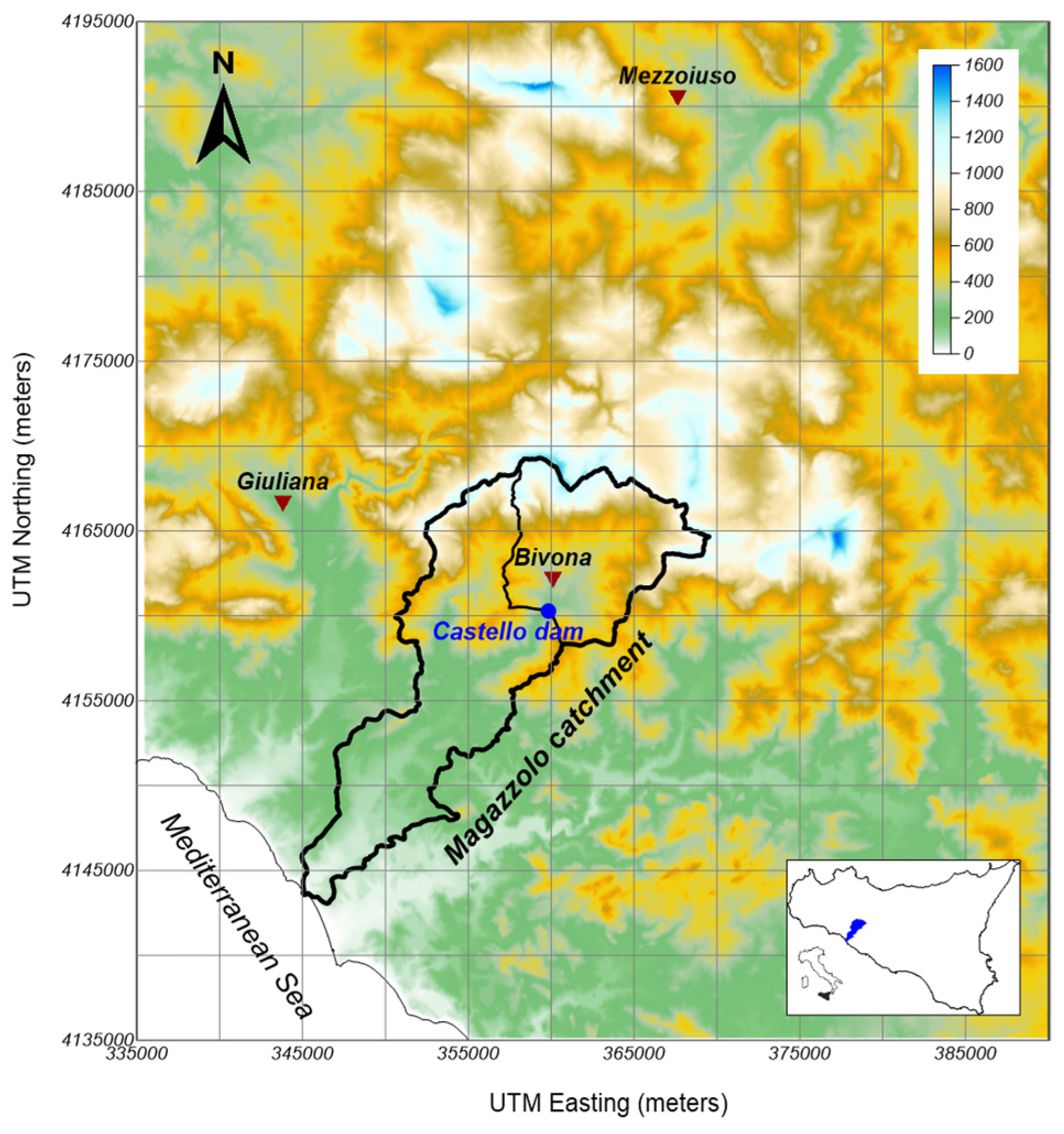
Castello dam is located in the southwestern part of Sicily (Italy), within the Magazzolo river catchment (Figure 1), and it is managed by the Sicily Regional Water Agency. According to the basic design information, the dam is characterized by a height of 50 m, a total volume of the reservoir of about 26 Mm3, and an impounded lake with an extension of 1.8 km2.
The dam is an earth-fill type with a clay core, and it is 792 m long at the top; it was built between 1976 and 1985, and it is one of the largest reservoirs in western Sicily. The upstream catchment of the dam, a sub-catchment of the Magazzolo River, is characterized by an area of 81 km2. The Digital Terrain Model (DTM) available for this area, extracted from a 20-m resolution DTM covering the whole Sicilian territory derived by an aerial photogrammetric survey, provides for the analysed sub-catchment at a maximum elevation of 1360 m above sea level (a.s.l.) and a minimum elevation of 250 m a.s.l. at Castello dam section. The normal water level of the reservoir is 293.65 m a.s.l., whereas the maximum water level is 296.65 m a.s.l.
Three rain gauge stations (Bivona, Giuliana, and Mezzojuso), managed by the Sicilian Agrometeorological Service (SIAS–Servizio Informativo Agrometeorologico Siciliano, www.sias.regione.sicilia.it) and located within or around the Magazzolo catchment (Figure 1), have been considered. For these stations, continuous rainfall time series, with a temporal resolution of 10 min, are available, respectively, for the period 2003–2020 for Bivona and Mezzoiuso and from 2005 to 2020 for the Giuliana rain gauge station. Moreover, a hydrometric ultrasonic gauge is installed on the dam crest measuring the lake water level and, indirectly, the flow discharges through the dam spillway.
2.2. The methodology
A Monte Carlo modelling chain (Figure 2) that includes hydrological simulations for synthetic flood hydrograph generation, reservoir routing, and hydraulic simulations for flood propagation and damage estimation has been implemented for the purposes of this study.
In particular, the developed modelling chain considers the following different steps: (a) Monte Carlo generation of ensembles of single synthetic rainfall events by using a stochastic bivariate model based on copulas that need sub-hourly rainfall time series as input; (b) generation of ensembles of single flood hydrographs by using a conceptual, fully distributed model fed with the above generated rainfall events; (c) flood hydrographs routing through the reservoir to obtain outflow hydrographs, for different reservoir conditions, in terms of initial water level (IWL); (d) flood propagation of the obtained outflow hydrographs and flood risk mapping through 2D hydraulic simulation; (e) flood damage modelling based on the results of the flood propagation model and on specific damage-depth curves. The modelling chain was entirely implemented in MATLAB environment with specific codes written for the purposes of the study.
2.2.1. Rainfall Generation Model
Single synthetic rainfall events have been generated by using a statistical model based on copulas theory, presented in detail in [21,30]. The model has a two-module structure: (a) volume-duration module for generation of the duration and the total volume of a single rainfall event; (b) storm temporal pattern module for the generation of the rainfall event profile.
For the model application, it is firstly required to identify independent rainfall events from the sub-hourly rainfall time series available as a function of the inter-event time that separates wet and dry periods. Rainfall time series can be represented as sequences of wet and dry periods where, during the wet period, a certain amount of rainfall is observed, while during the dry period, no rain (or less than a threshold value) is observed.
Between all the extracted rainfall events, it is then necessary to specify and select those considered as hydrologically “significant” for the possible formation of a flood, i.e., the maximum events. Kao and Govindaraju [31] stated how the definition of annual maximum events for multivariate problems is somewhat ambiguous. As matter of fact, extreme rainfall events could be defined as storms that have both high volume and peak intensity. Therefore, the definition of extreme rainfall based on events with annual maximum joint cumulative probability has been considered in this study.
For generating the duration and the total volume of a single rainfall event, a bivariate analysis on the empirical data needs to be performed by applying the well-known theory of copulas. For this application, Frank and Gumbel–Hougard copulas have been considered and adapted to the observed pairs of total volume and duration. Their formulas are respectively:
where θ is the parameter of the two copula functions estimated using the inversion of the Kendall’s coefficient method.
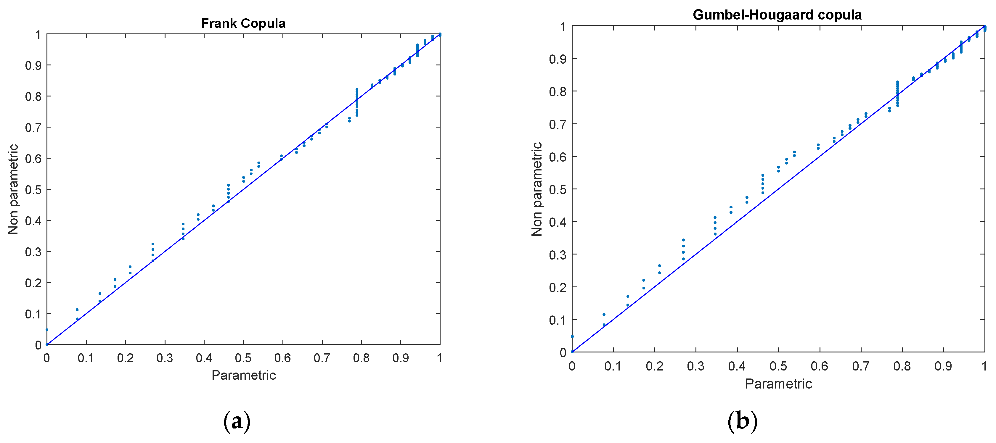
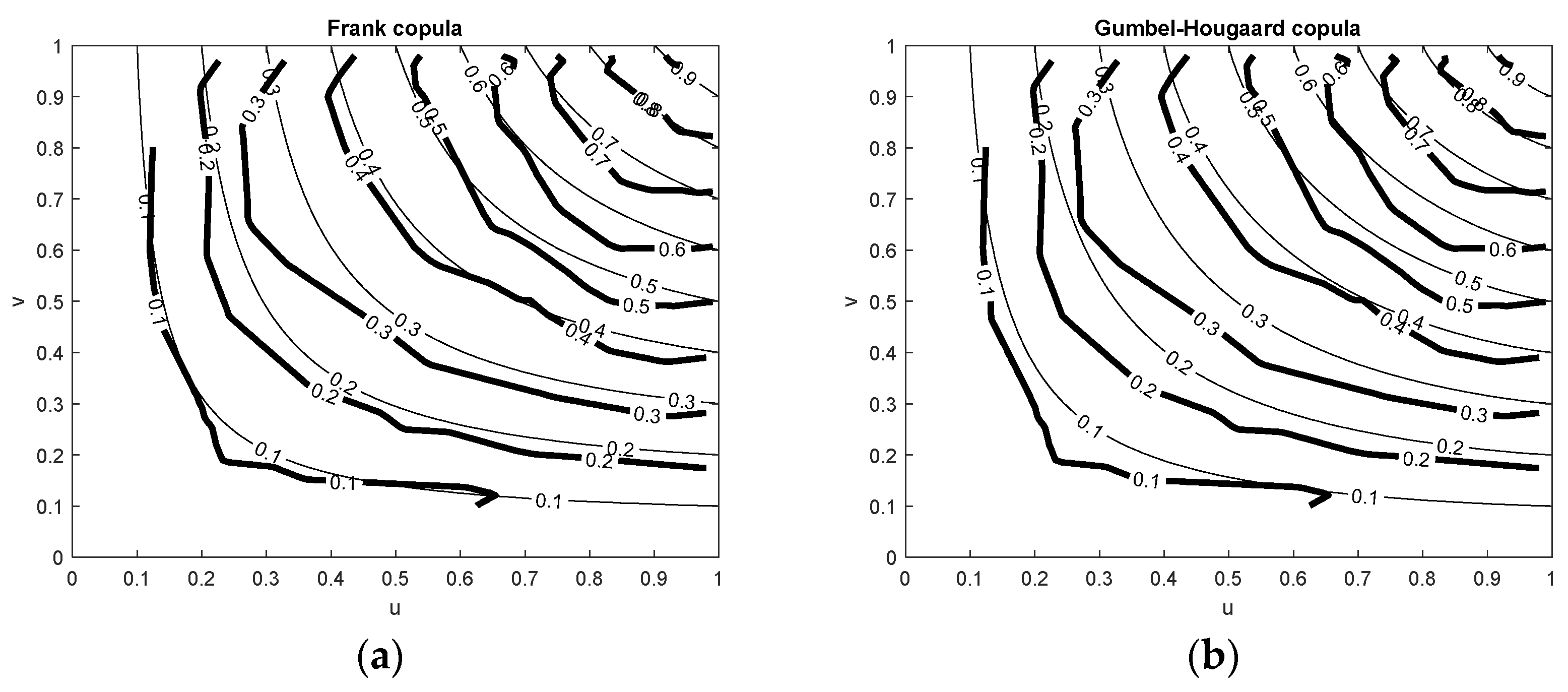
In order to select the copula that best represents the dependence structure of the empirical data, two graphical tools are used; primarily, the goodness of fit is tested by means of the K-plot, as defined by Genest and Rivest [32], where the values of the parametric function K(z) for both copulas are calculated and compared with the nonparametric function Kn(z) derived from the empirical data. The second graphical test is, instead, performed by comparing the level curves (isolines) of the theoretical copulas and those of the empirical ones.
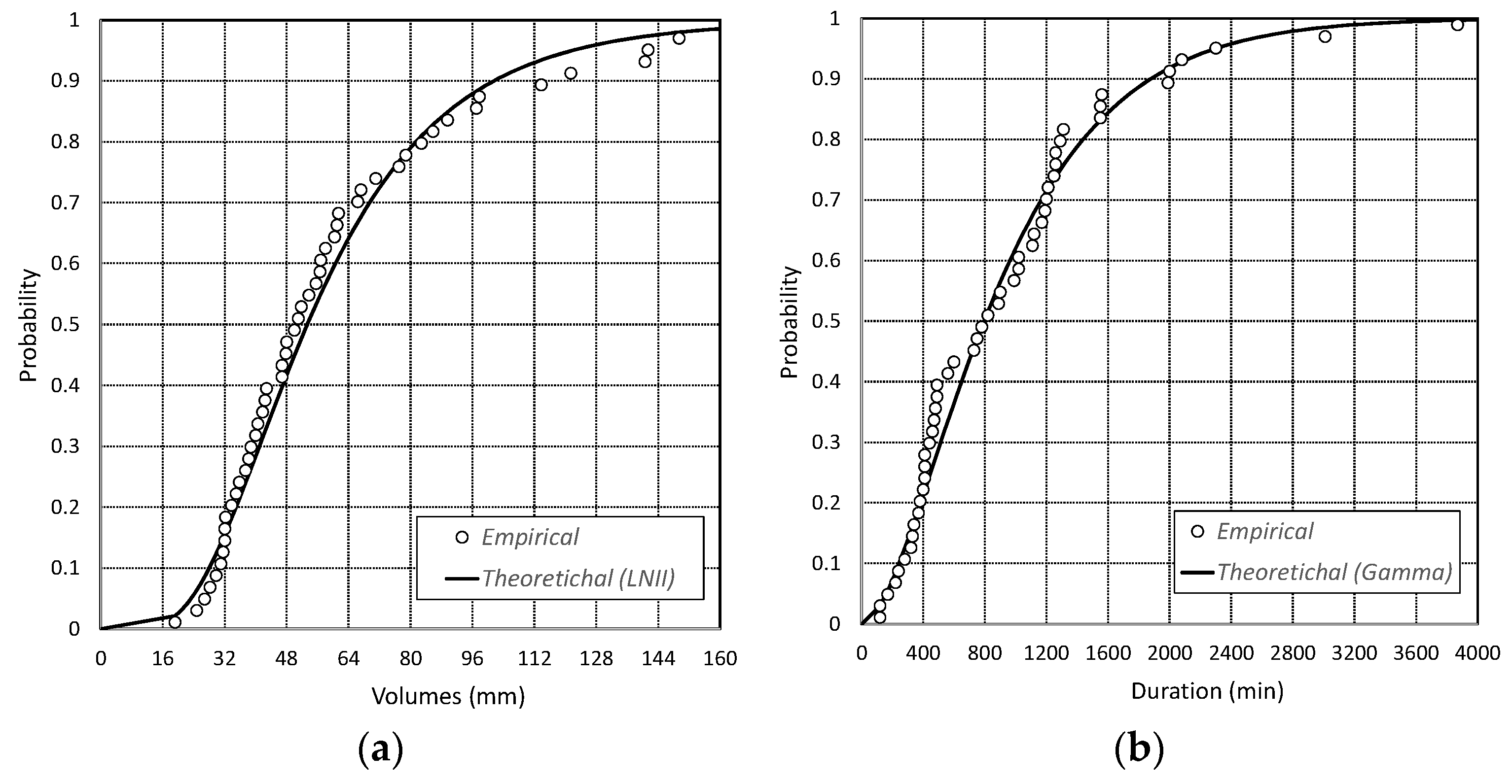
Finally, the use of copulas requires the determination of marginal distributions based on univariate data. For this application, the fitting of several statistical distributions is performed by applying the maximum likelihood method, and the best fitted distribution is selected using various criteria, i.e., the Akaike information criterion (AIC), the relative root mean square error (RRMSE) and the Anderson–Darling test [33,34].
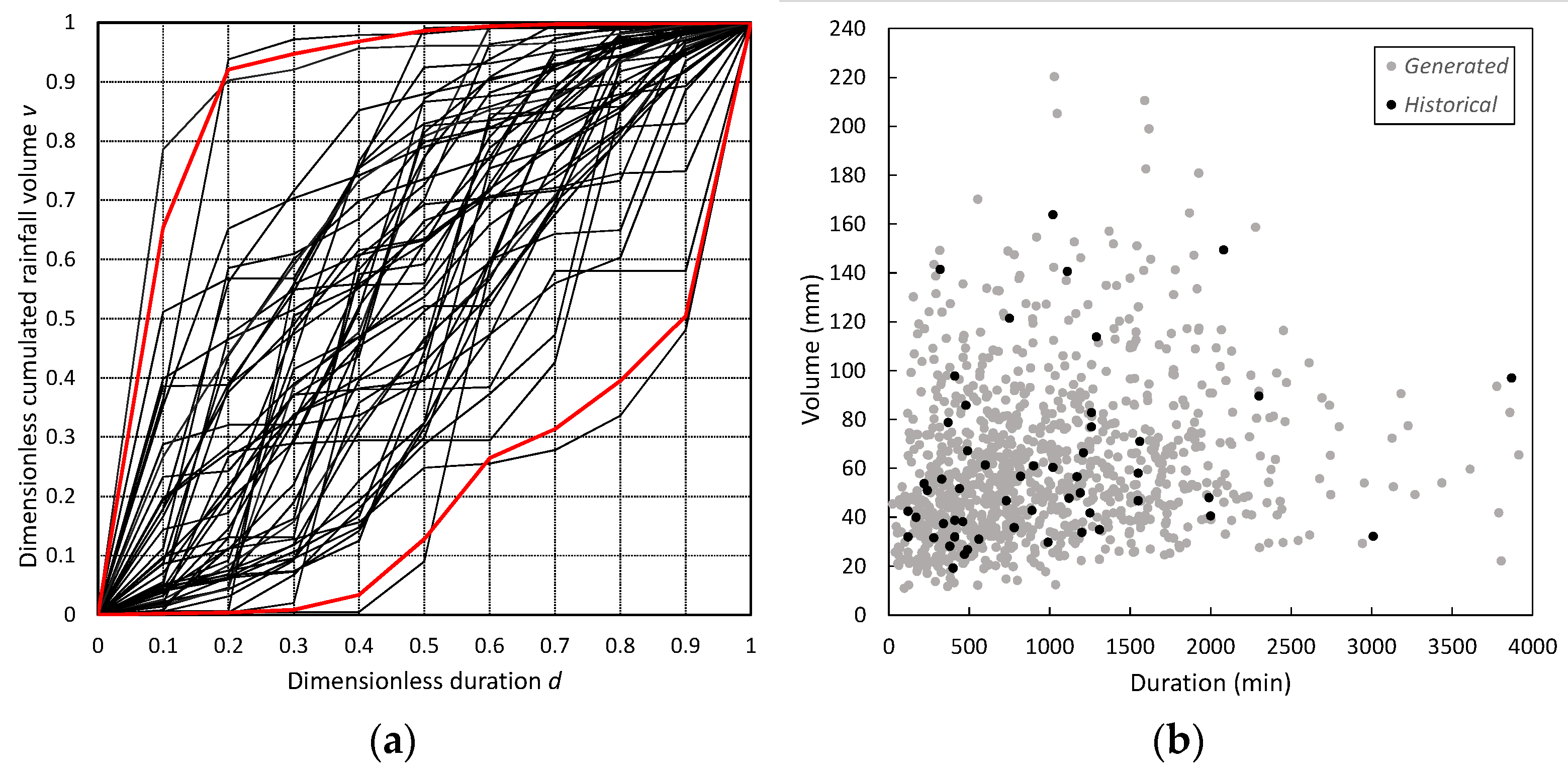
For the generation of the rainfall event profile, the storm temporal pattern module is implemented. This approach uses the mass curves concept [35] defined as the normalized cumulative rainfall volume versus normalized time since the event start. According to this definition, each event can be represented by pairs of two dimensionless variables, namely d and v, defined as: (a) d = t/D is the event dimensionless duration obtained by dividing the generic time t by the total rainfall duration D; (b) v = h(t)/V is event dimensionless cumulated rainfall volume obtained as the fraction of the cumulated rainfall depth h(t) at generic time t by the total rainfall volume V.
For the generation of the single synthetic rainfall event, dimensionless hyetograph can be chosen with a random picking from the set of the historical shapes.
2.2.2. Flood Hydrographs Generation Model
Generated rainfall events are used as input for the derivation of the correspondent flood hydrographs entering the reservoir by applying the fully distributed conceptual rainfall-runoff model proposed by Candela et al. [30].
The model has a grid-based structure where each small element (cell) has a distinct hydrological response, treated separately, but incorporates interactions with bordering cells. It is based on the linear kinematic mechanism for the transfer of the effective rainfall from different contributing areas to the catchment outlet and on a nonlinear approach for the rainfall excess calculation. In addition, model input represented by single rainfall events is considered in a fully distributed form.
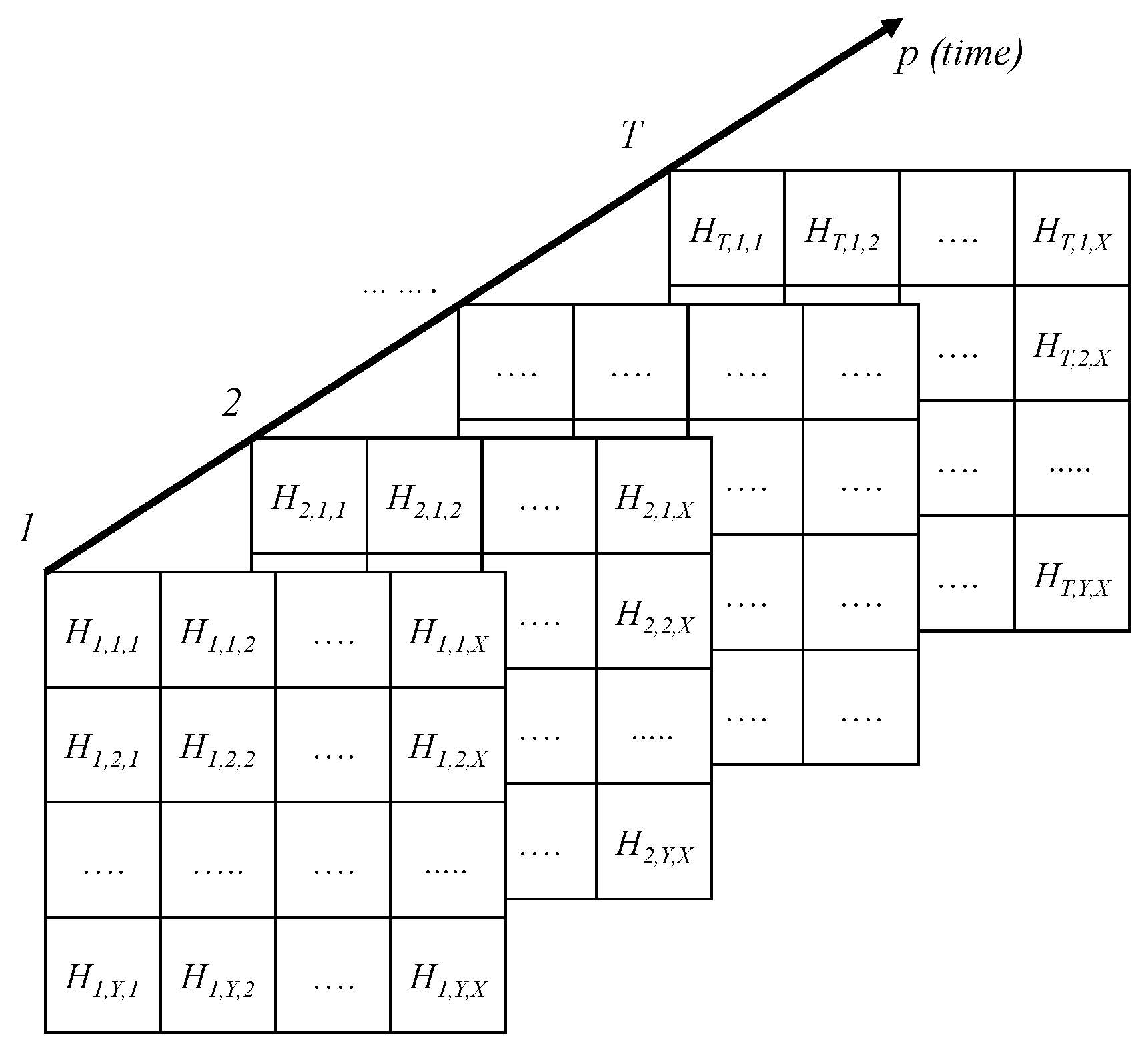
The linear mechanism is represented by the distributed hydrological response function (UH) in a kinematic form, and it is described through a three-dimensional matrix H(m, n, p) (Figure 3), which represents the space-time distribution of contributing areas (isochrones areas).
The subscripts m = 1, 2 …, X and n = 1, 2, …, Y describe the elements of the matrix, while X and Y are the number of cells in which the catchment is discretized in the directions x and y. The subscript p = 1, 2, …, T counts the number of intervals (with T = Ω/∆t) in which the simulation time Ω is discretized. The matrix element Hm,n,p represents the area of generic cell (m, n) characterized by a concentration time ϑc(m,n).
For the evaluation of the concentration time at cell scale, the Wooding formula [36] is implemented in the model:
where Lm,n→,out [m] is the hydraulic path length between the centroid of the (m, n) cell and the outlet section of the catchment, km,n→,out [m1/3/s] is the Strickler roughness for the same path, sm,n→,out [m/m] is its slope, and rm,n [m/s] is the average rainfall intensity for the rainfall event over the (m, n) cell.
The SCS-CN method proposed by USDA Soil Conservation Service [37] has been implemented in this model for the rainfall excess calculation (hydrological losses). The grid-based structure of the model allows direct incorporation of CN spatial distribution maps, taking into account the spatial variation of land use, soil type, and antecedent moisture conditions. The SCS-CN equations are also implemented in the model in a dynamic form [38], as the input rainfall can be variable in time:
and
Using above equations, a three-dimensional matrix Pe (q, m, n) of the same structure of H matrix, which represents the space-time distribution of excess rainfall, can be obtained.
The subscript q = 1, 2 …, N counts the elements of the matrix to N, which represents the number of steps in which the rainfall event of duration D (with N = D/∆t) is divided.
To compute the direct runoff hydrograph at the catchment outlet, the model solves the discrete convolution equation for a linear system as matrix multiplication:
where Q is the flood hydrograph vector with dimension N + T − 1.
Using this model for the generation of the flood hydrographs requires the calibration of the model parameters. Calibration is necessary for only two parameters: the coefficient c in the SCN-CN rainfall excess calculation formula (Equation (4)) and the Strickler roughness coefficient k in the Wooding formula (Equation (3)). For the other model parameters, i.e., path lengths L, average slopes s and the CN values, a calibration is not required, as their values can be directly extracted from the Digital Elevation Model and the CN map of the catchment. Finally, several metrics have been adopted to verify the goodness of the calibration.
2.2.3. Reservoir Routing Model for Discharged Hydrographs Derivation
The inflow hydrographs derived above have to be routed through the reservoir to obtain the outflow hydrographs from the spillway (peak flows, volumes, and total duration) for different initial conditions in terms of initial water level (IWL).
In level pool routing, the upstream discharge may be expressed explicitly in terms of the downstream discharge and of the channel or reservoir characteristics. Level pool routing is based on the continuity equation:
where Qin(t) is the inflow hydrograph, Qout[W(t)] is the outflow hydrograph, and W(t) is the reservoir storage. The problems for which this equation is applicable are given by Yevjevich [39]. Equation (7) has been here solved numerically using a fourth-order Runge–Kutta method implemented in a Matlab routine [39]. Particularly, the inflow discharge can be simulated using rainfall-runoff models, and the outflow discharge can be computed using spillway rating curve as follows:
where Cd is the discharge coefficient assumed equal to 0.385, Le is the effective length of spillway crest, and 𝐻 is the head on the spillway crest. The effective length of the spillway crest can be computed as follows:
where Ln is the net length of the crest, Np is the number of the piers, Kp is the pier contraction coefficient, and Ka is the abutment contraction coefficient.
2.2.4. Flood Propagation Modelling Downstream Reservoir
Outflow hydrographs for different reservoir conditions are then used for deriving flood hazard and risk maps downstream.
The Multilevel Flood Propagation 2D (MLFP-2D) model [40,41] has been implemented, in this study, to carry out flood inundation scenarios downstream. It is a hyperbolic model, whose details can be found in Candela and Aronica [42], based on the Saint–Venant equations and where the convective inertial terms are neglected. The model is based on two equations, conservative mass and momentum equations, which depend on the hydraulic resistances that can be calculated in function of the Manning–Strickler parameter. Both equations are solved using a finite-element triangular mesh that needs to be used to carry out model simulations.
Manning’s roughness coefficient is the unique calibration parameter involved in the MLFP-2D propagation model, and for its calibration, the procedure described in detail in Candela and Aronica [42] has been followed.
2.2.5. Flood Damage Evaluation
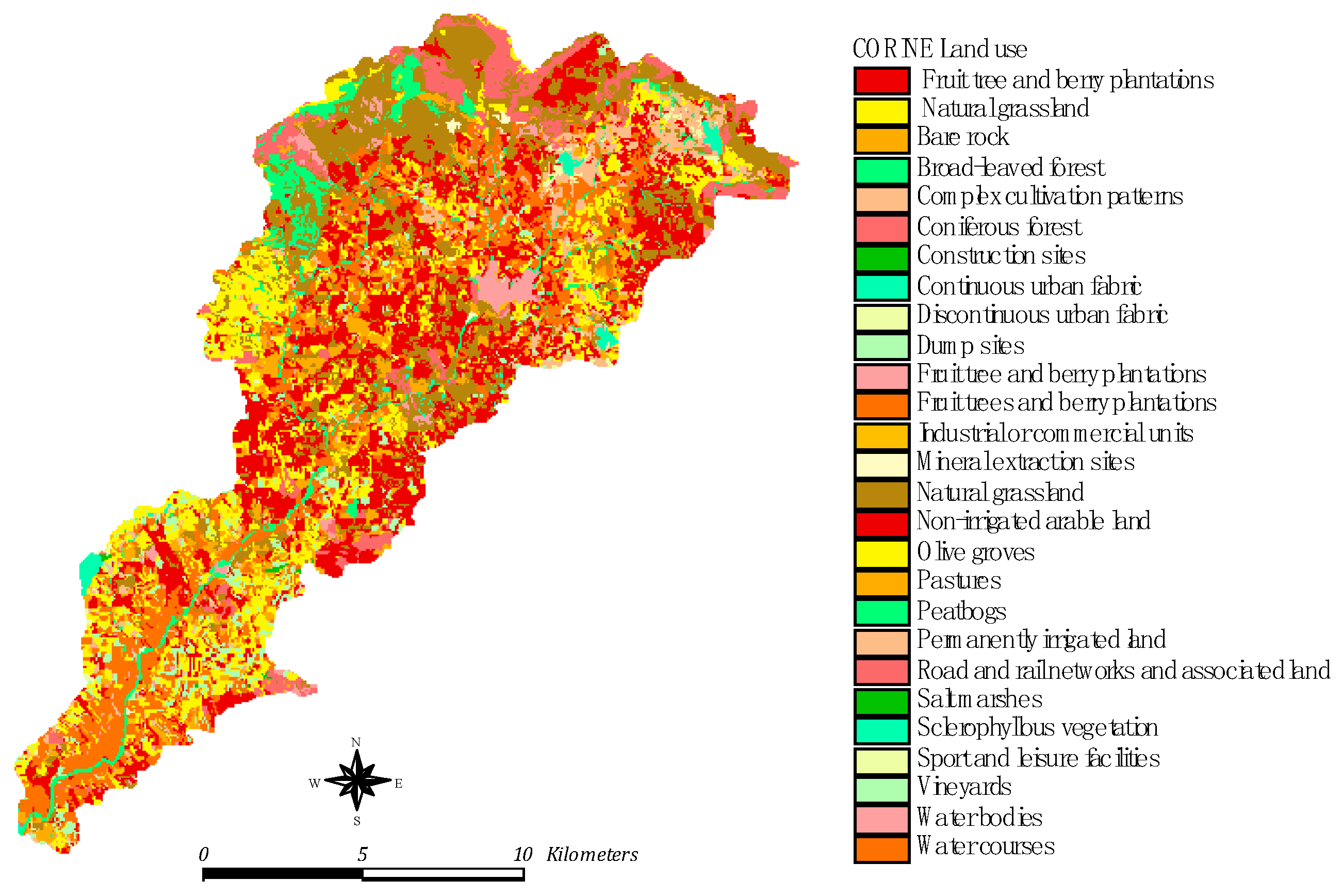
The evaluation of the total damage caused by the flooding in downstream area has been achieved by means of specific damage–depth curves (damage curves) derived considering that this area is mainly for agricultural use, as shown by the land use classes based on the CORINE Land Cover map for the Magazzolo catchment (Figure 4).
In this case, the damage is linked to the spatial and temporal variability of the flood that can cause strong loss of production and yield. For this reason, potential damage functions have been here obtained based on the methodology proposed by the Joint Research Centre, which considers both “new” costs (replacement) and productivity costs [29], starting from the knowledge of the land use classes of the area of interest.
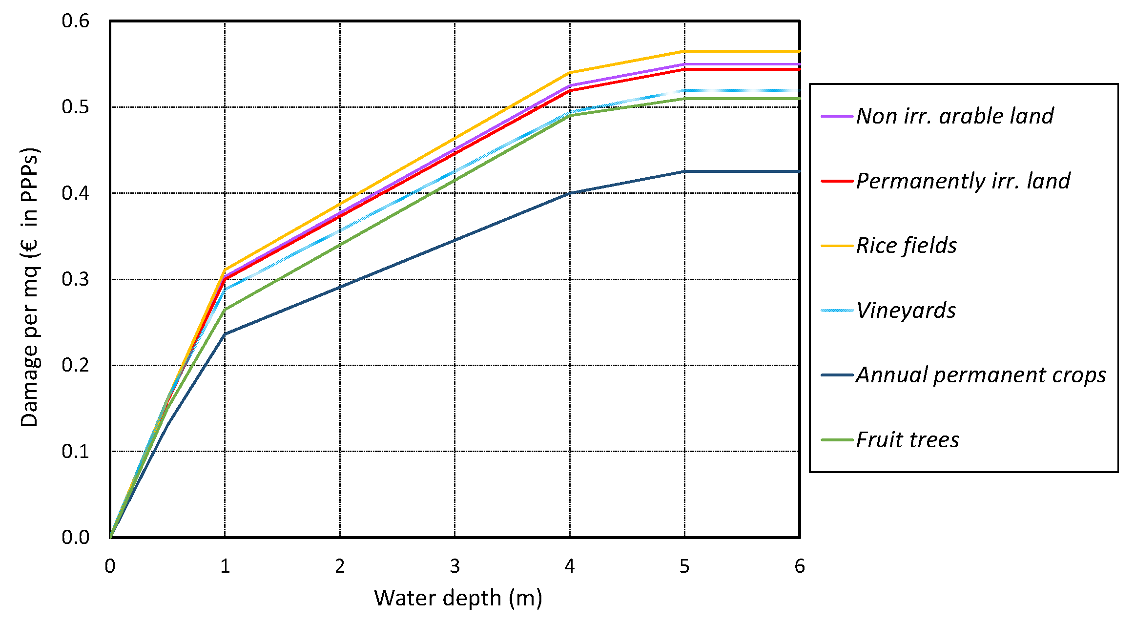
Following this approach, firstly, the depth–damage functions, expressing the damage in terms of Euros in Purchasing Power parities (PPPs) proposed by Rusmini [43], have been considered (Figure 5). These functions relate nine depths (0, 0.5, 1, 1.5, 2, 3, 4, 5, and 6 or more meters) to the corresponding damage rates (from 0 to 1) for the most important land use classes of the CORINE Land Cover map. Consequently, these curves represent the relationship between water depth in the inundated area and the damage, in percent, for m2 for the same purchasing power parity (PPP).
The determination of the PPP is then carried out through the consultation of the National Institute of Agricultural Economics (INEA) reports [44] in order to estimate the average values of agricultural land with the same purchasing power for the study area (Table 1).
As the damage is expressed in relative units (per square meter), the calculation can be carried out by averaging the water depths at finite element scale. Specifically, a unique value for each element can be calculated by averaging the three nodal values, and given the element area and the crop category associated with the element, the total damage is obtained.
3. Results
Single synthetic rainfall events have been generated, following the procedure described in Section 2.2.1, on the basis of a sample of 52 historical maximum annual rainfall events extracted as follows.
An inter-event time equal to 5 h was initially adopted to separate wet and dry periods in each sub-hourly rainfall series analysed; then, the events with annual maximum joint cumulative probability were selected for each analysed year for Bivona, Giuliana, and Mezzoiuso rain gauge stations. Finally, as all these rain gauges are in the same hydrologically homogeneous area [45,46], subsequent statistical analyses have been performed by aggregating all the selected events in a unique sample of 52 rainfall events whose main characteristics are reported in Table 2.
Gumbel–Hougard and Frank copula families were adapted to the observed pairs of total volume and duration. The θ parameter of these two copula functions was estimated using the inversion of Kendall’s coefficient method, and the results so obtained are reported in Table 3.
To select the copula that best represents the dependence structure of the empirical data, as specified in paragraph 2.2.1, two graphical tools have been used. Firstly, the goodness of fit was tested by means of the K-plot, as defined by Genest and Rivest [32]. In this plot (Figure 6), the values of the parametric function K(z) for both copulas were calculated and compared with the non-parametric function Kn(z) derived from the empirical data.
A second graphical test was performed by comparing the level curves (isolines) of the theoretical copulas and those of the empirical copula (Figure 7).
Both tests confirmed how the Frank copula is well suited to describing the dependence structure between the empirical variables considered, and hence, it has been used for the rainfall generation model.
Moreover, the use of copulas requires the determination of marginal distributions based on univariate data. Therefore, fitting of several statistical distributions (i.e., Exponential, Gamma, Lognormal (LNII), Weibull, and General Extreme Values (GEV)) was considered by applying the maximum likelihood method, and the best fitted distribution was selected using various criteria. Simulations returned LNII distribution as the best marginal distribution for the rainfall volumes (Figure 8a) and Gamma distribution as the best marginal distribution for the rainfall duration (Figure 8b).
Temporal patterns of rainfall (event profile), for each event, were characterized using the mass curves concept, and the dimensionless hyetographs so derived for the selected annual maximum rainfall events (Figure 9a) have been used for the derivation of synthetic rainfall.
With these assumptions, 1500 synthetic rainfall events have been generated. This number was chosen as a trade-off between the statistical significance of the generated variables and the burden of the computational time requested for the simulations. About this, the comparison with the historical events is reported in Figure 9b, showing a good reproducibility of the rainfall main characteristics.
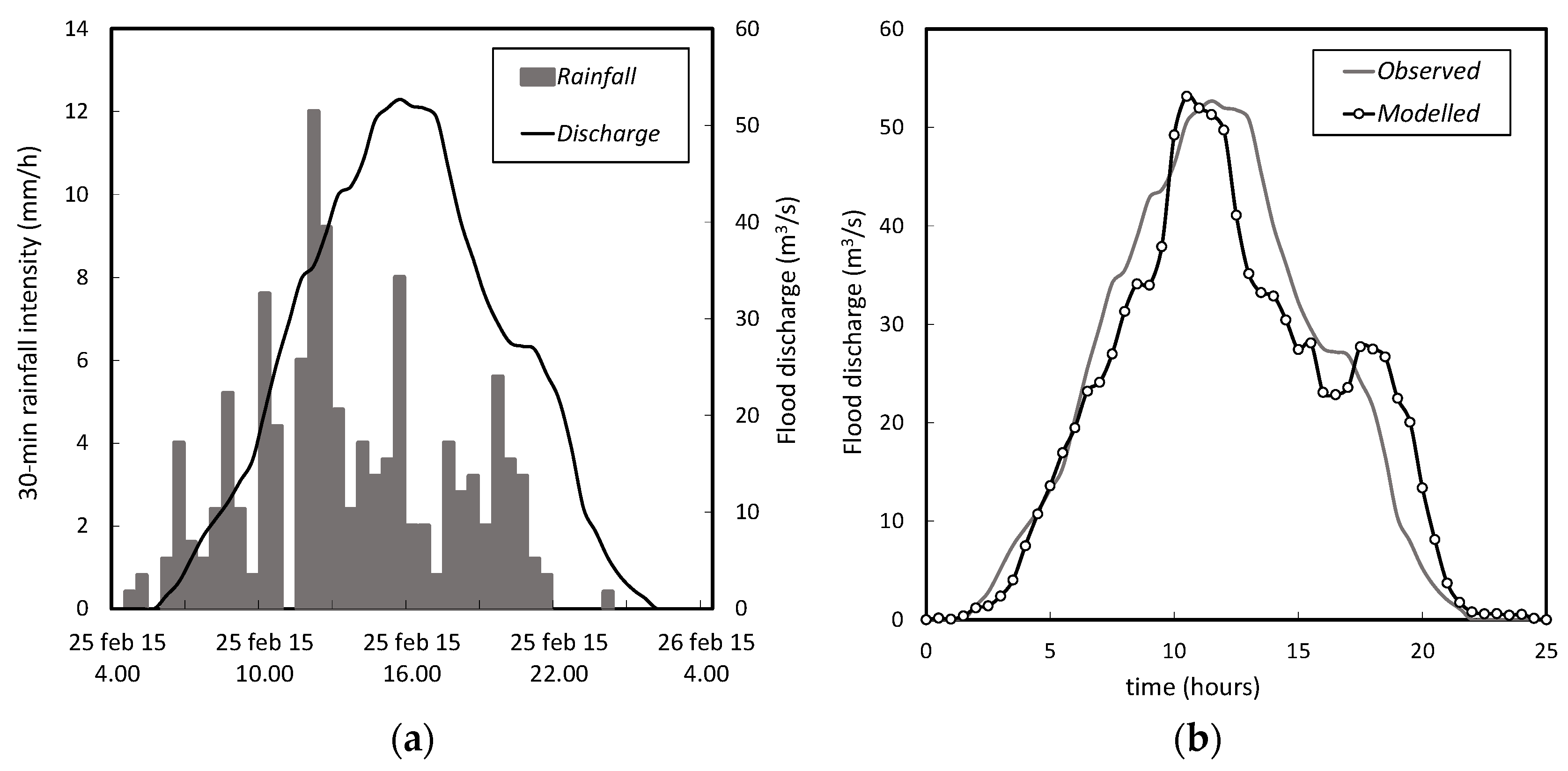
The events so generated have been used as input for the derivation of the correspondent flood hydrographs entering the reservoir by applying the flood hydrographs generation model illustrated in Section 2.2.2. The model was calibrated using the software PEST [47] on the basis of the outflow flood hydrograph through the spillway recorded by the water level gauge installed on the crest of the dam and of the rainfall recorded by the three rain gauges of the measurement network for the event of 25–26 February 2015 (Figure 10a). The parameter estimation software PEST, which is a combination of gradient descent and Newton’s method, implements the Gauss–Levenberg–Marquardt method [48,49] for parameter estimation and uncertainty analysis.
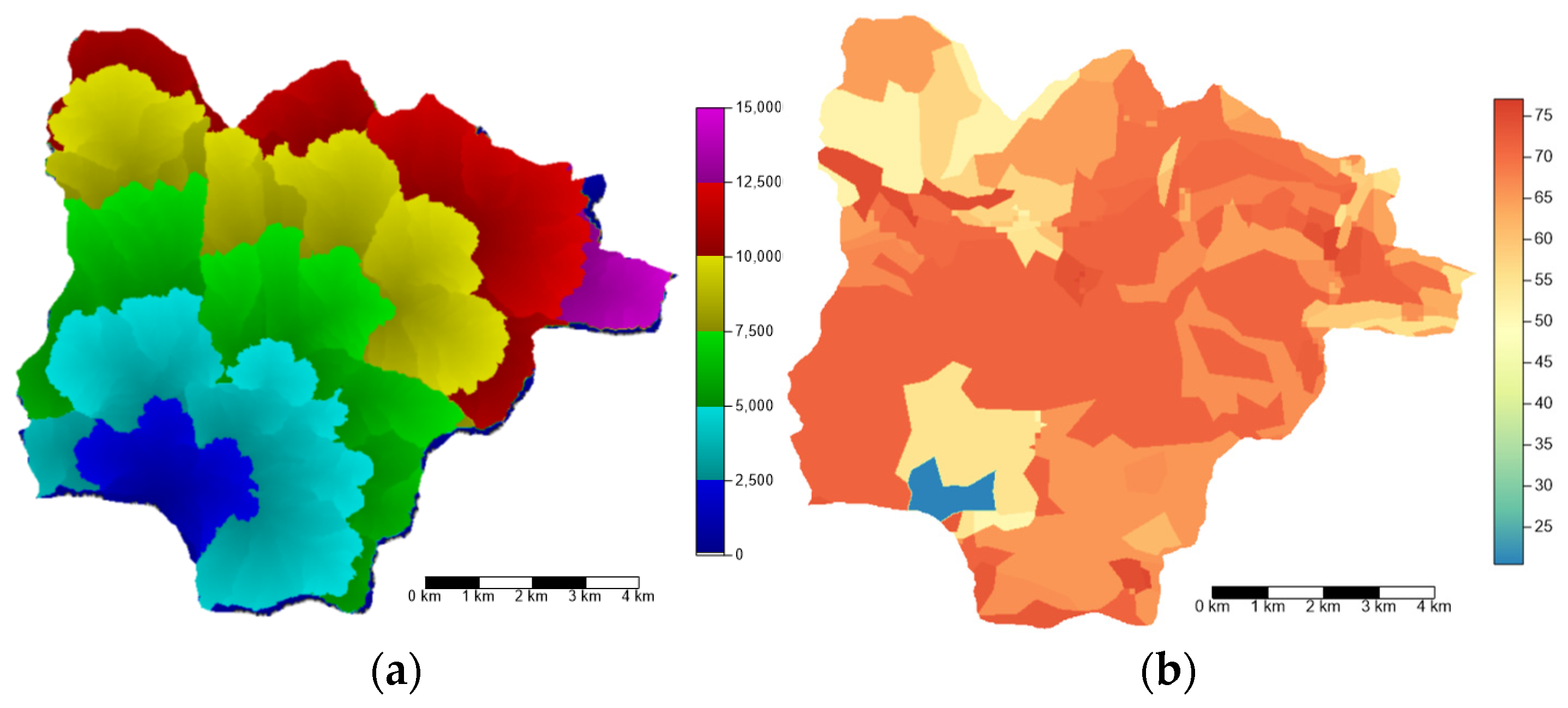
As mentioned before, the coefficient c in the SCN-CN rainfall excess calculation formula (Equation (4)) and Strickler roughness coefficient k in the Wooding formula (Equation (3)) are the only parameters that required calibration. The other model parameters needed to run the model have, instead, been extracted from the Digital Elevation Model (20 m resolution) and the CN map (100 m resolution available for the CNII value) available for the sub-catchment (Figure 11).
More in detail, path lengths L (Figure 11a) and, consequently, average slopes s, have been extracted from the DTM map (Figure 1), whereas the CN values have been derived starting from the CN map available for the moderately wet soil moisture condition (CNII) (Figure 11b).
Considering that most of the catchments in Sicily are small, with flashy hydrological response and a proneness to flash floods formation, especially when the soil is totally wet (CNIII condition), CN values considered to run the model are those relative to totally wet soil condition (CNIII values), derived from the CNII values as follows [50]:
Despite the distributed nature of the Strickler roughness coefficient k, for the sake of simplicity, a “lumped” value was calibrated by considering a spatial average over the whole catchment.
Final results of the model calibration are reported in Figure 10b, where the observed and modelled flood hydrographs are plotted for the optimal values of the two parameters. Their final values are c = 0.155 and k = 19.8 m1/3/s, respectively.
The calibration efficiency was measured through several metrics; in particular, we selected the Mean Absolute Error (MAE), the Root mean Standard deviation Ratio (RSR), and the Nash-Sutcliffe (NSE) indexes to compare errors between observed and estimated discharge values. As a result, we obtained a MAE equal to 3.647 m3/s, a RSR index equal to 0.283, and a Nash-Sutcliffe index equal to 0.921, with an error in-peak discharge of 0.94% and in-flood volume of −4.96%.
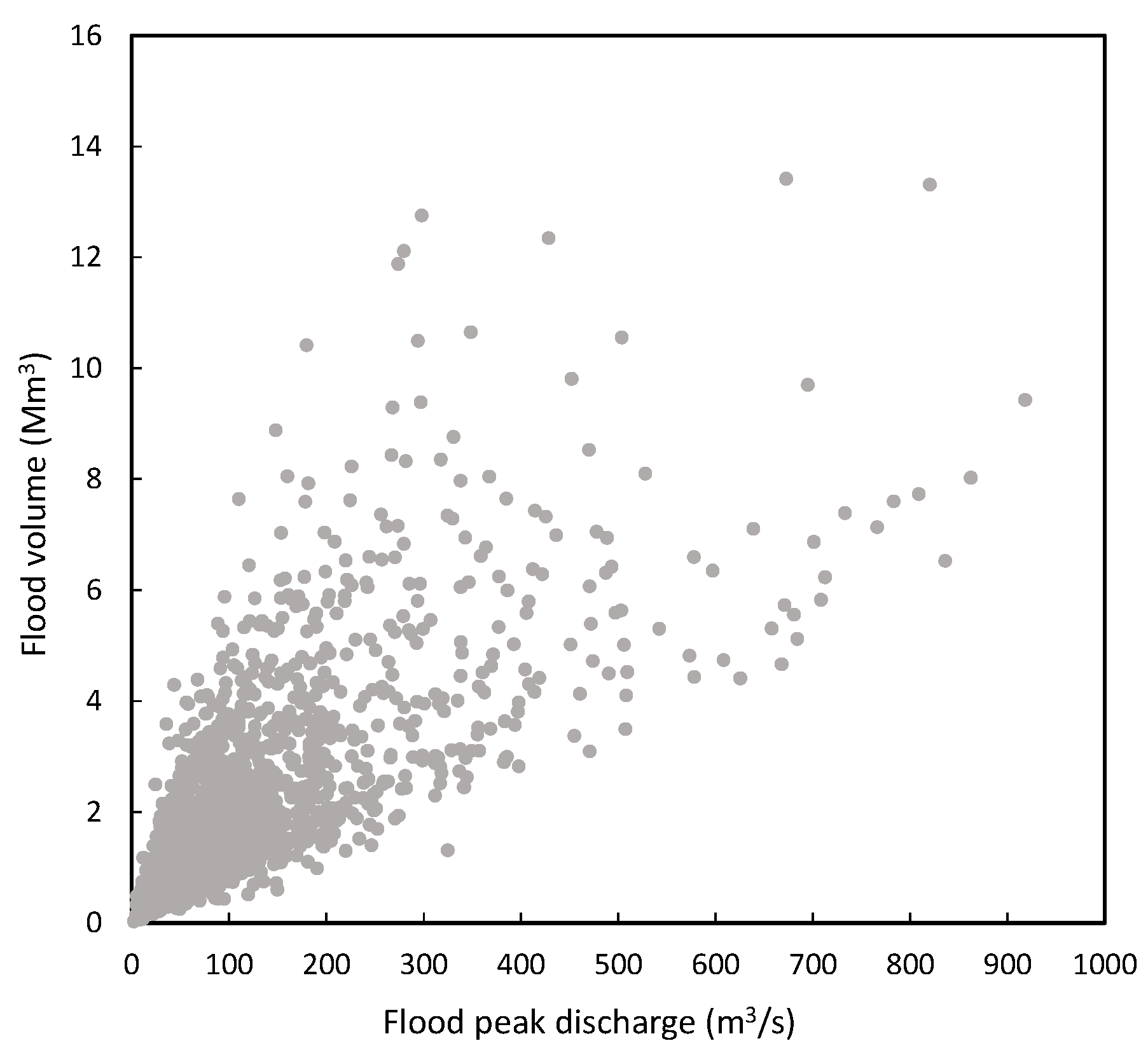
The flood hydrograph generation module was, hence, used to generate 1500 flood hydrographs (Figure 12) entering the reservoir correspondent to the 1500 synthetic rainfall events above generated.
The inflow hydrographs routed through the reservoir, by applying the procedure described in Section 2.2.3, allowed obtaining the outflow hydrographs from the spillway (peak flows, volumes, and total duration) for different initial conditions in terms of Initial Water Level (IWL). For a broader analysis, two specific values were chosen: the highest (IWL1), equal to 293.65 m a.s.l., corresponding to normal water level of the reservoir and the lowest (IWL2), equal to 290.00 m a.s.l., corresponding to the most frequent observed level at the dam.
The outflow hydrographs, for the two different reservoir conditions, were finally used for deriving flood hazard and risk maps downstream from the Castello dam by applying MLFP-2D model and for flood damage evaluation.
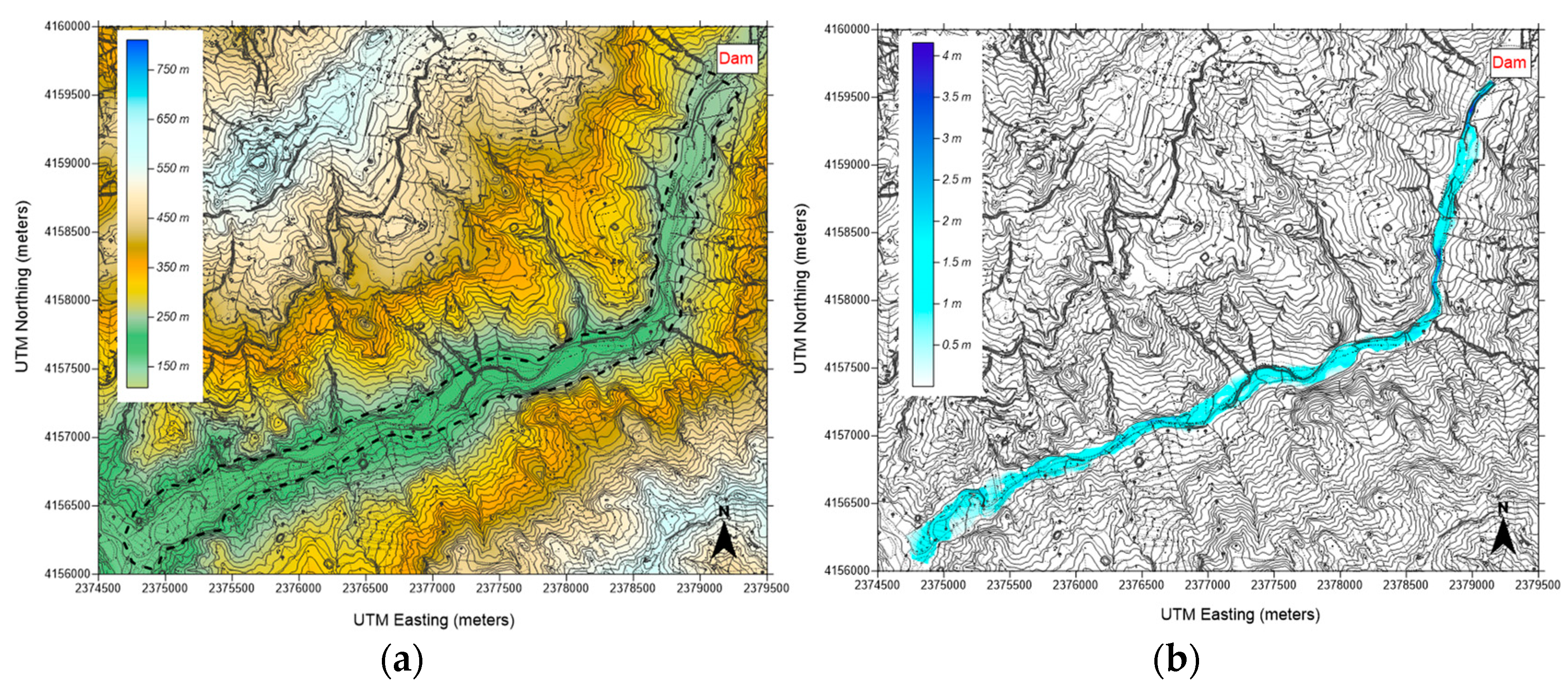
The model equations have been solved using a finite-element triangular mesh. The mesh covers a domain area of 1.68 km2 downstream, discretized into 25.436 nodes and 49.278 elements. The terrain elevations for the study area were derived starting from a 2-m resolution DTM interpolated from a LIDAR survey available for the floodplain. Manning’s roughness coefficient was the unique calibration parameter involved in the propagation model; particularly, one coefficient for each triangular element can be chosen but, lacking a robust basis for allowing the roughness coefficient to vary, the entire triangular domain was divided into two principal regions—the floodplain area and the river—and for both regions, a calibrated Manning roughness coefficient was considered (0.037 s.m−1/3 for the river and 0.051 s.m−1/3 for the floodplain area). As an example, in Figure 13, the domain DTM (Figure 13a) and the flood inundated area for a given reservoir condition (Figure 13b), corresponding to normal water level in the reservoir, are reported.
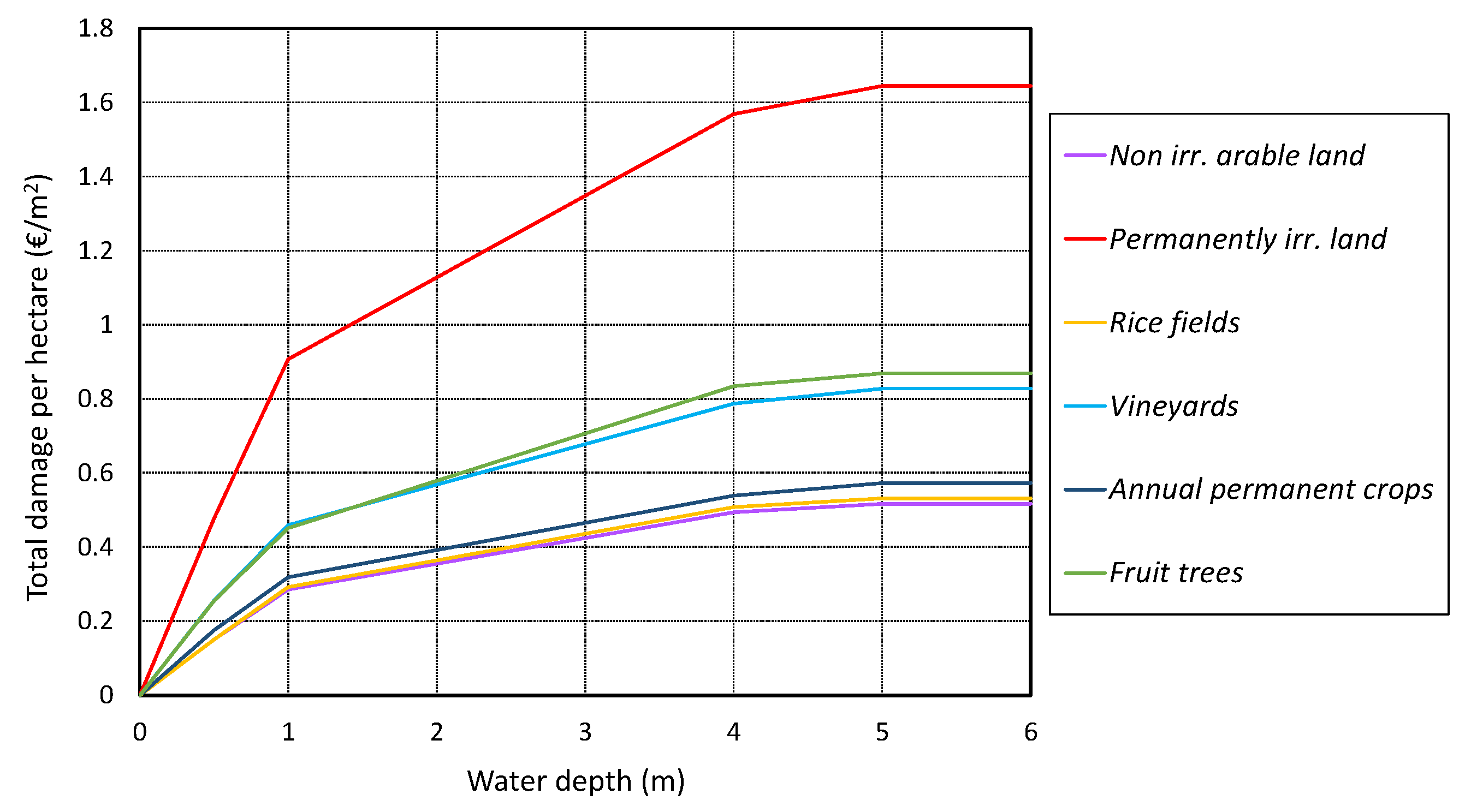
The evaluation of the total damage caused by the flooding has been carried out by means of the specific damage–depth curves (damage curves) derived, as presented, in Section 2.2.5. Particularly, the damage–depth curves illustrated in Figure 5 have been suitably combined with the average values per m2 of agricultural land with the same purchasing power of the area where the study area is located, obtaining the damage curves representing the total damage per m2 in function of the water depth for the main agricultural landcover classes of the Magazzolo floodplain (Figure 14).
Finally, for each simulation, the total direct flood damage has been calculated for the two initial reservoir conditions (IWL1 and IWL2) considered.
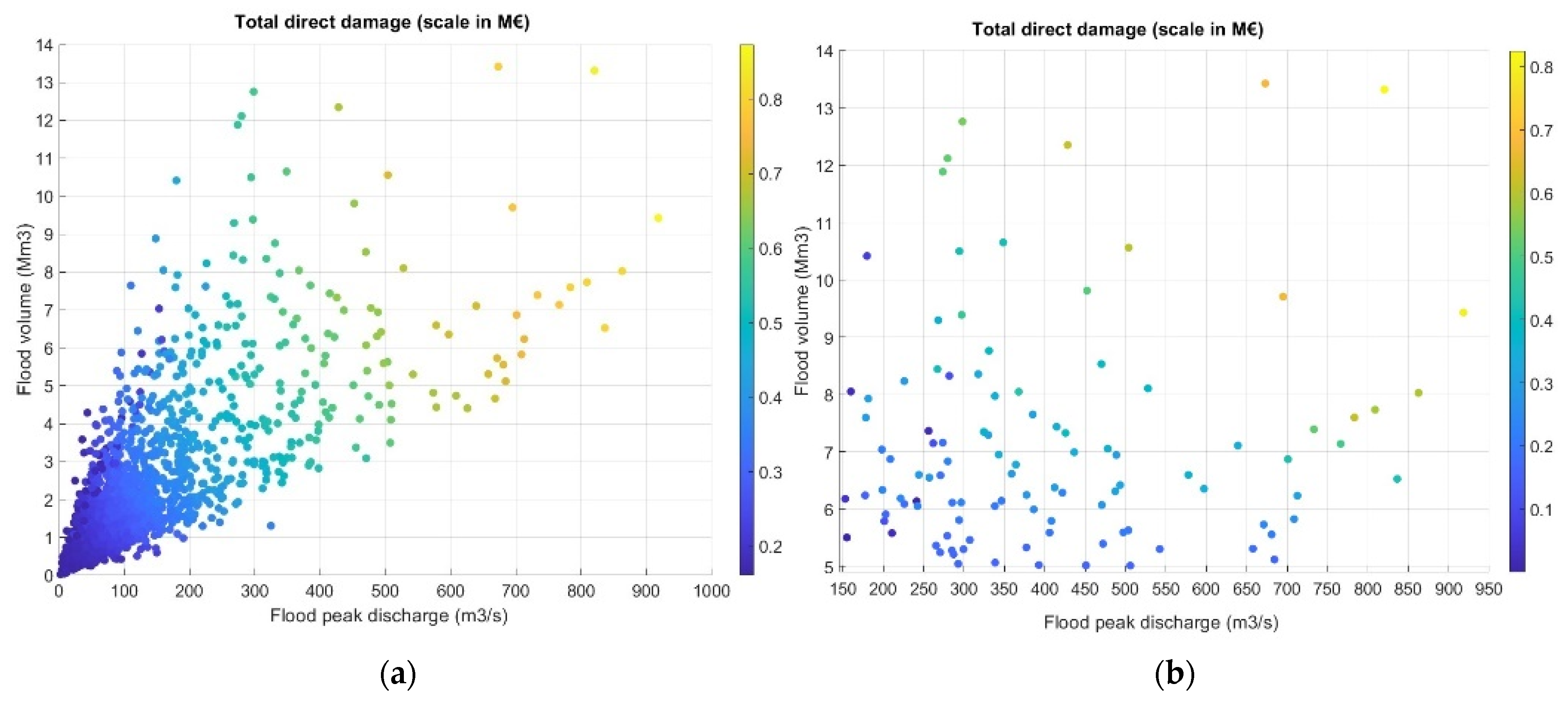
In Figure 15, the results of the simulations are reported by plotting, with a scale of colour for the total damage, the dots representing the inflow hydrographs (flood peak discharge–flood volume pairs, specifically). The choice of representing these results in relation to the hydrological forcing to the reservoir is due to the technical/practical aspects, which the proposed procedure intends to address.
For these aspects, which will be further discussed, and for a better visualization, the clouds of points have been visualized as smooth surfaces obtained by a 2-D spatial interpolation (Figure 16).
4. Discussion
By looking more in detail into Figure 15, a strong correlation between the total damage and the flood peaks–volume pairs, in the case of IWL1 condition, is revealed, while this correlation is definitively weaker (or likely absent) in the case IWL2 condition.
This behaviour appears to be reasonable in the view of the two specific conditions: for IWL1 condition, the reduction effect due to the reservoir volume is lower than the IWL2 condition and, hence, all the flood hydrographs are routed, discharged downstream from the dam, and the original correlation structure between hydrographs characteristics (peak discharges and volumes) is essentially preserved. In the IWL2 condition, instead, some hydrographs are retained and not routed through the reservoir. This results in less events producing flood inundations and, generally, lower values of total damages.
Interpolated 2-D “damage surfaces” (Figure 16), corresponding to the two IWL conditions, can be used for quantifying the expected damage downstream from the dam for a given input hydrograph by simply entering the plot with a given pair of flood peak-volume.
In both cases, the higher damage level can be observed only when both variables (flood peaks and volume) show the major values. Again, this evidence is clearer for the IWL1 condition than IWL2, due to the fact of the influence of the reservoir (flood control) on the routed hydrographs.
In detail, these surfaces clearly show these specific results, whereas the regions characterized by higher values of total damage are more extended in IWL1 condition than IWL2 and vice versa. Regions characterized by lower values of total damage are more extended in IWL2 condition than IWL1.
To better clarify these statements, consider two distinct hydrological scenarios for the reservoir, i.e., the 50-yrs and 100-yrs return time input hydrographs, with each characterized by a specific pair of peak discharge and volume, obtained by bivariate analysis of the generated sample. The corresponding values are: 653.0 m3/s and 7.92 Mm3 for 50-yrs return time; 824.0 m3/s and 8.99 Mm3 for 100-yrs return time.
Now, by entering the surface plot with these two pair, it is possible to evaluate the damage, which is equal to 811,862 Euro for IWL1 condition and 560,765 Euro for IWL2 condition, both for 100-yrs return time. Similar results can be obtained for 50-yrs return time, as shown in Table 4.
Hence, lowering the reservoir level produces a difference of about 30.9% in total direct damage downstream from the dam for 100-yrs return time and 51.8% for 50-yrs return time.
As matter of fact, the comparison between the results for the two IWL conditions shows how it is possible to have a direct insight on the role which the reservoir plays in protecting the downstream floodplain and to prove its capability to control inundation and reduce direct flood damage.
Damage surfaces allow us to quantify the impact of the different reservoir conditions on the direct flood damage downstream, and they can help the flood risk managers in setting up specific operation rules for the reservoir in order to mitigate the impact of extreme hydro meteorological events.
5. Conclusions
In this study, an efficient and reliable Monte Carlo modelling chain for producing flood risk scenarios downstream to a dam, as a function of the initial water level in the reservoir, has been presented. The methodology allows us to quantify the total direct flood damage in a floodplain downstream of a dam through the generation of ensembles of single rainfall events by using a copula based model, of flood hydrographs by using a conceptual fully distributed rainfall-runoff model, as well as of discharged hydrographs from a reservoir routing and a two-dimensional hydraulic flood propagation model.
Flood damage scenarios have been produced for the Magazzolo river floodplain, downstream the Castello dam in Sicily, using 1500 stochastic extreme rainfall events. Damage analysis for the different flood damage scenarios revealed how the reservoir rules operation (in terms of initial reservoir conditions or IWL) strongly influences the effects of flooding in the downstream floodplain. In particular, the performed analysis reveals how there is a strong correlation between the total damage and the flood peaks–volume pairs in the case of normal water level conditions, while the correlation is definitively weaker in the case of a more frequent water level.
Finally, the a priori knowledge of the possible damage associated with a forecasted or measured flood event, as a function of the water level of the reservoir, can be very useful in case of flood warning to help the Water Authorities to quantify the potential downstream damage and to make appropriate decisions, i.e., lowering the reservoir level for the mitigation of the damage downstream.
Author Contributions
Conceptualization, G.B., A.C. and G.T.A.; methodology, G.B., A.C. and G.T.A.; software, G.B., A.C. and G.T.A.; validation, G.B. and G.T.A.; formal analysis, G.B. and G.T.A.; resources, G.B.; data curation, G.B.; writing—original draft preparation, G.B. and A.C.; writing—review and editing, G.B. and G.T.A.; visualization, G.B.; supervision, G.T.A. All authors have read and agreed to the published version of the manuscript.
Funding
This research received no external funding.
Institutional Review Board Statement
Not applicable.
Informed Consent Statement
Not applicable.
Data Availability Statement
Not applicable.
Acknowledgments
Author would like to thank the Sicilian Agrometeorological Service (SIAS) for having provided the rainfall data and the Dam Service of Sicilian Region for the Castello dam data.
Conflicts of Interest
The authors declare no conflict of interest.
References
- Guo, S.; Zhang, H.; Chen, H.; Peng, D.; Liu, P.; Pang, B. A reservoir flood forecasting and control system for China / Un système chinois de prévision et de contrôle de crue en barrage. Hydrol. Sci. J. 2004, 49, 959–972. [Google Scholar] [CrossRef]
- Bruwier, M.; Erpicum, S.; Pirotton, M.; Archambeau, P.; Dewals, B.J. Assessing the operation rules of a reservoir system based on a detailed modelling chain. Nat. Hazards Earth Syst. Sci. 2015, 15, 365–379. [Google Scholar] [CrossRef] [Green Version]
- Iveti´c, D.; Milašinovi´c, M.; Stojkovi´c, M.; Šoti´c, A.; Charbonnier, N.; Milivojevi´c, N. Framework for Dynamic Modelling of the Dam and Reservoir System Reduced Functionality in Adverse Operating Conditions. Water 2022, 14, 1549. [Google Scholar] [CrossRef]
- Tedla, M.G.; Cho, Y.; Jun, K. Flood Mapping from Dam Break Due to Peak Inflow: A Coupled Rainfall–Runoff and Hydraulic Models Approach. Hydrology 2021, 8, 89. [Google Scholar] [CrossRef]
- Dobson, B.; Wagener, T.; Pianosi, F. An argument-driven classification and comparison of reservoir operation optimization methods. Adv. Water Resour. 2019, 128, 74–86. [Google Scholar] [CrossRef]
- Gabriel-Martin, I.; Sordo-Ward, A.; Garrote, L.; Granados, I. Hydrological Risk Analysis of Dams: The Influence of Initial Reservoir Level Conditions. Water 2019, 11, 461. [Google Scholar] [CrossRef] [Green Version]
- Luino, F.; Tosatti, G.; Bonaria, V. Dam Failures in the 20th Century: Nearly 1000 Avoidable Victims in Italy Alone. J. Environ. Sci. Eng. 2014, 3, 19–31. Available online: http://www.cnr.it/prodotto/i/285435 (accessed on 15 November 2022).
- Bocchiola, B.; Rosso, R. Safety of Italian dams in the face of flood hazard. Adv. Water Resour. 2014, 71, 23–31. [Google Scholar] [CrossRef]
- Direttiva del Presidente del Consiglio dei Ministri 8 luglio 2014. Indirizzi Operativi Inerenti All’attività di Protezione Civile Nell’ambito dei Bacini in cui Siano Presenti Grandi Dighe. Available online: https://www.dighe.eu/normativa/allegati/2014_Direttiva_PCM_8-07.pdf (accessed on 8 July 2014). (In Italian).
- Koutsoyiannis, D.; Economou, A. Evaluation of the parameterization-simulation-optimization approach for the control of reservoir systems. Water Resour. Res. 2003, 39, 1170–1434. [Google Scholar] [CrossRef] [Green Version]
- Huang, L.; Xiang, L.; Fang, H.; Yin, D.; Si, Y.; Wei, J.; Liu, J.; Hu, X.; Zhang, L. Balancing social, economic and ecological benefits of reservoir operation during the flood season: A case study of the Three Gorges Project, China. J. Hydrol. 2019, 572, 422–434. [Google Scholar] [CrossRef]
- Giuliani, M.; Lamontagne, J.R.; Reed, P.M.; Castelletti, A. A State-of-the-Art Review of Optimal Reservoir Control for Managing Conflicting Demands in a Changing World. Water Resour. Res. 2021, 57, e2021WR029927. [Google Scholar] [CrossRef]
- Papathanasiou, C.; Serbis, D.; Mamassis, N. Flood mitigation at the downstream areas of a transboundary river. Water Utility J. 2013, 3, 33–42. [Google Scholar]
- Hardesty, S.; Shen, X.; Nikolopoulos, E.; Anagnostou, E. A Numerical Framework for Evaluating Flood Inundation Hazard under Different Dam Operation Scenarios—A Case Study in Naugatuck River. Water 2018, 10, 1798. [Google Scholar] [CrossRef] [Green Version]
- Zhou, T.; Jin, J. Comparative analysis of routed flood frequency for reservoirs in parallel incorporating bivariate flood frequency and reservoir operation. J. Flood Risk. Manag. 2021, 14, e12705. [Google Scholar] [CrossRef]
- Shen, G.; Lu, Y.; Zhang, S.; Xiang, Y.; Sheng, J.; Fu, J.; Fu, S.; Liu, M. Risk dynamics modeling of reservoir dam break for safety control in the emergency response process. Water Supply 2021, 21, 1356–1371. [Google Scholar] [CrossRef]
- Acreman, M.C. A simple stochastic model of hourly rainfall for Farnborough, England. Hydrol. Sci. J. 1990, 35, 119–148. [Google Scholar] [CrossRef] [Green Version]
- Cameron, D.; Beven, K.; Tawn, J. An evaluation of three stochastic rainfall models. J. Hydrol. 2000, 228, 130–149. [Google Scholar] [CrossRef]
- Vandenberghe, S.; Verhoest, N.E.C.; Buyse, E.; De Baets, B. A stochastic design rainfall generator based on copulas and mass curves. Hydrol. Earth Syst. Sci. 2010, 14, 2429–2442. [Google Scholar] [CrossRef] [Green Version]
- Volpi, E.; Fiori, A. Design event selection in bivariate hydrological frequency analysis. Hydrol. Sci. J. 2012, 57, 1506–1515. [Google Scholar] [CrossRef]
- Brigandì, G.; Aronica, G.T. Generation of Sub-Hourly Rainfall Events through a Point Stochastic Rainfall Model. Geosciences 2019, 9, 226. [Google Scholar] [CrossRef] [Green Version]
- Salvadori, G.; De Michele, C.; Kottegoda, N.T.; Rosso, R. Extremes in Nature. An Approach Using Copulas; Springer: Dordrecht, The Netherlands, 2007. [Google Scholar]
- Genest, C.; Favre, A.C. Everything you always wanted to know about copula modeling but were afraid to ask. J. Hydrol. Eng. ASCE 2007, 12, 347–368. [Google Scholar] [CrossRef]
- Requena, A.I.; Mediero, L.; Garrote, L. A bivariate return period based on copulas for hydrologic dam design: Accounting for reservoir routing in risk estimation. Hydrol. Earth Syst. Sci. 2013, 17, 3023–3038. [Google Scholar] [CrossRef] [Green Version]
- Balistrocchi, M.; Orlandini, S.; Ranzi, R.; Bacchi, B. Copula-based modeling of flood control reservoirs. Water Resour. Res. 2017, 53, 9883–9900. [Google Scholar] [CrossRef]
- Rizwan, M.; Guo, S.; Yin, J.; Xiong, F. Deriving Design Flood Hydrographs Based on Copula Function: A Case Study in Pakistan. Water 2019, 11, 1531. [Google Scholar] [CrossRef] [Green Version]
- Tan, Q.; Mao, Y.; Wen, X.; Jin, T.; Ding, Z.; Wang, Z. Copula-based modeling of hydraulic structures using a nonlinear reservoir model. Hydrol. Res. 2021, 52, 1577. [Google Scholar] [CrossRef]
- Klein, B.; Schumann, A.H.; Pahlow, M. Copulas—New Risk Assessment Methodology for Dam Safety. In Flood Risk Assessment and Management; Schumann, A.H., Ed.; Springer: Dordrecht, The Netherlands, 2010; pp. 149–185. [Google Scholar] [CrossRef]
- Huizinga, J.; De Moel, H.; Szewczyk, W. Global Flood Depth-damage Functions. JRC Technical Report. Available online: https://publications.jrc.ec.europa.eu›JRC105688 (accessed on 30 May 2022).
- Candela, A.; Brigandì, G.; Aronica, G.T. Estimation of synthetic flood design hydrographs using a distributed rainfall-runoff model coupled with a copula-based single storm rainfall generator. Nat. Hazards Earth Syst. Sci. 2014, 14, 1819–1833. [Google Scholar] [CrossRef] [Green Version]
- Kao, S.-C.; Govindaraju, R.S. Probabilistic structure of storm surface runoff considering the dependence between average intensity and storm duration of rainfall events. Water Resour. Res. 2007, 43, W06410. [Google Scholar] [CrossRef]
- Genest, C.; Rivest, L. Statistical inference procedures for bivariate Archimedean copulas. J. Amer. Statist. Assoc. 1993, 88, 1034–1043. [Google Scholar] [CrossRef]
- Maidment, D.R. Handbook of Hydrology; McGraw-Hill International: New York, NY, USA, 1992. [Google Scholar]
- Kottegoda, N.T.; Rosso, R. Applied Statistics for Civil and Environmental Engineers; Blackwell Publishing Ltd.: Oxford, UK, 2008. [Google Scholar]
- Huff, F. Time Distribution Rainfall in Heavy Storms. Water Resour. Res. 1967, 3, 1007–1019. [Google Scholar] [CrossRef]
- Wooding, R.A. A hydraulic model for the catchment stream problem: 1.-Kinetic wave theory. J. Hydrol. 1965, 3, 254–267. [Google Scholar] [CrossRef]
- US Department of Agriculture. Soil Conservation Service, National Engineering Handbook, Hydrology: Sec.4; US Department of Agriculture: Washington, DC, USA, 1986. [Google Scholar]
- Chow, V.T.; Maidment, D.R.; Mays, L.W. Applied Hydrology; McGraw-Hill: New York, NY, USA, 1998. [Google Scholar]
- Yevjevich, V.M. Analytical integration of the differential equation for water storages. J. Res. Nat. Bureau Stand.-B. Math. Math. Phys. 1959, 63, 43–52. Available online: https://nvlpubs.nist.gov/nistpubs/jres/63B/jresv63Bn1p43_A1b.pdf (accessed on 30 May 2022). [CrossRef] [Green Version]
- Aronica, G.T.; Tucciarelli, T.; Nasello, C. 2D Multilevel Model for Flood Wave Propagation in Flood-Affected Areas. J. Water Resour. Plan. Manag.-ASCE 1998, 124, 210. [Google Scholar] [CrossRef]
- Aronica, G.T.; Candela, A. Derivation of flood frequency curves in poorly gauged catchments using a simple stochastic hydrological rainfall-runoff model. J. Hydrol. 2007, 347, 132–142. [Google Scholar] [CrossRef]
- Candela, A.; Aronica, G.T. Probabilistic Flood Hazard Mapping Using Bivariate Analysis Based on Copulas. ASCE-ASME J. Risk Uncertain. Eng. Syst. Part A Civ. Eng. 2017, 3, A4016002-A1. [Google Scholar] [CrossRef]
- Rusmini, M. Pan-European Flood Hazard and Damage Assessment; Evaluation of a New If-SAR Digital Terrain Model for Flood Depth and Flood Extent Calculation. Available online: https://webapps.itc.utwente.nl/librarywww/papers_2009/msc/aes/rusmini.pdf (accessed on 30 May 2022).
- INEA. Il Valore della Terra. Available online: https://rica.crea.gov.it/download.php?id=938 (accessed on 30 May 2022).
- Bonaccorso, B.; Aronica, G.T. Estimating Temporal Changes in Extreme Rainfall in Sicily Region (Italy). Water Resour. Manag. 2016, 30, 5651–5670. [Google Scholar] [CrossRef]
- Bonaccorso, B.; Brigandì, G.; Aronica, G.T. Regional sub-hourly extreme rainfall estimates in Sicily under a scale invariance framework. Water Resour. Manag. 2020, 34, 4363–4380. [Google Scholar] [CrossRef]
- Doherty, J. PEST: Model Independent Parameter Estimation; Watermark Numerical Computing: Brisbane, Australia, 2010. Available online: https://www.epa.gov/sites/default/files/documents/PESTMAN.PDF (accessed on 30 May 2022).
- Levenberg, K. A method for the solution of certain non-linear problems in least squares. Q. Appl. Math. 1944, 2, 164–168. [Google Scholar] [CrossRef] [Green Version]
- Marquardt, D. An algorithm for least-squares estimation of non-linear parameters. J. Soc. Ind. Appl. Math. 1963, 11, 431–441. [Google Scholar] [CrossRef]
- Ponce, V.; Hawkins, R. Runoff Curve Number: Has It Reached Maturity? J. Hydrol. Eng. 1996, 1, 11–19. [Google Scholar] [CrossRef]
Figure 1.
Magazzolo River catchment.

Figure 2.
Layout of the proposed procedure.

Figure 3.
Matrix representation of IUH.

Figure 4.
Land use classes based on the CORINE Land Cover map for the Magazzolo catchment.

Figure 5.
Depth–damage functions of main agricultural landcover classes for Italy (after [43]).
Figure 5.
Depth–damage functions of main agricultural landcover classes for Italy (after [43]).

Figure 6.
Q-Q plot (nonparametrically estimated Kn(z) versus parametrically estimated K(z)) for: (a) Frank copula; (b) Gumbel–Hougard copula.
Figure 6.
Q-Q plot (nonparametrically estimated Kn(z) versus parametrically estimated K(z)) for: (a) Frank copula; (b) Gumbel–Hougard copula.

Figure 7.
Comparison between the level curves of the theoretical copulas (thin lines) and the empirical copulas (thick lines) for: (a) Frank copula; (b) Gumbel–Hougaard copula.
Figure 7.
Comparison between the level curves of the theoretical copulas (thin lines) and the empirical copulas (thick lines) for: (a) Frank copula; (b) Gumbel–Hougaard copula.

Figure 8.
Goodness of fit assessment of marginal distribution of: (a) rainfall volumes; (b) durations.
Figure 8.
Goodness of fit assessment of marginal distribution of: (a) rainfall volumes; (b) durations.

Figure 9.
(a) Dimensionless hyetographs for the selected events (thick red lines for 5% and 95% percentiles); (b) Scatter plot of 1500 values generated by the model and the empirical data.
Figure 9.
(a) Dimensionless hyetographs for the selected events (thick red lines for 5% and 95% percentiles); (b) Scatter plot of 1500 values generated by the model and the empirical data.

Figure 10.
Flood event of 25–26 February 2015: (a) Observed flood hydrograph and rainfall; (b) comparison between observed and modelled hydrographs.
Figure 10.
Flood event of 25–26 February 2015: (a) Observed flood hydrograph and rainfall; (b) comparison between observed and modelled hydrographs.

Figure 11.
Castello dam catchment: (a) Path length map scale in meters); (b) CNII spatial distribution map.
Figure 11.
Castello dam catchment: (a) Path length map scale in meters); (b) CNII spatial distribution map.

Figure 12.
Scatter plot of 1500 pairs obtained through the flood hydrograph generation module.

Figure 13.
MLFP-2D model implementation: (a) layout of the model domain, including 2-m resolution DTM and the domain boundary (black dotted line); (b) inundated area for a single random generated hydrograph and a given initial water level reservoir condition (IWL1).
Figure 13.
MLFP-2D model implementation: (a) layout of the model domain, including 2-m resolution DTM and the domain boundary (black dotted line); (b) inundated area for a single random generated hydrograph and a given initial water level reservoir condition (IWL1).

Figure 14.
Damage curves for agricultural classes in Magazzolo floodplain.

Figure 15.
Total direct damage (in MEuro) for different IWL conditions: (a) 293.65 m a.s.l. water level (IWL1); (b) 290.00 m a.s.l. water level (IWL2).
Figure 15.
Total direct damage (in MEuro) for different IWL conditions: (a) 293.65 m a.s.l. water level (IWL1); (b) 290.00 m a.s.l. water level (IWL2).

Figure 16.
Spatial interpolation for the total direct damage (damage surfaces) for different IWL conditions: (a) 293.65 m a.s.l water level (IWL1); (b) 290.00 m a.s.l. water level (IWL2).
Figure 16.
Spatial interpolation for the total direct damage (damage surfaces) for different IWL conditions: (a) 293.65 m a.s.l water level (IWL1); (b) 290.00 m a.s.l. water level (IWL2).


Table 1.
Average values per mq of agricultural land with the same purchasing power in Sicily.
| Main Agricultural Surface | Average Values per M2 (Euros) |
|---|---|
| Non irrigable arable land | 0.9403 |
| Fruit trees | 1.9614 |
| Permanently irrigated land | 3.0224 |
| Vineyards | 1.5923 |
| Annual and permanent crops | 1.3474 |
Table 2.
Main characteristics of the selected maximum rainfall events.
| Duration (min) | Volume (mm) | Iavg (mm/h) | Imax,30′ (mm/h) | |
|---|---|---|---|---|
| Length of record (years) | 17 (2003–2020) | |||
| Number of events | 52 | |||
| Max | 3870 | 163.8 | 26.51 | 84.80 |
| Min | 120 | 19.2 | 0.64 | 9.20 |
| Mean | 955.58 | 60.84 | 6.12 | 37.76 |
| Standard deviation | 743.96 | 34.35 | 5.38 | 20.01 |
Table 3.
θ parameter for the analysed copulas.
| Copula | θ |
|---|---|
| Gumbel–Hougard | 1.2427 |
| Frank | 2.1407 |
Table 4.
Total damage in Euro for different hydrological input and IWLs.
| Return Time | Qmax/Vtot | IWL1 (293.65 m) | IWL2 (290.00 m) |
|---|---|---|---|
| 50 years | 653.0 m3/s | € 735,738 | € 354,563 |
| 7.92 Mm3 | |||
| 100 years | 824.0 m3/s | € 811,862 | € 560,765 |
| 8.99 Mm3 |
Disclaimer/Publisher’s Note: The statements, opinions and data contained in all publications are solely those of the individual author(s) and contributor(s) and not of MDPI and/or the editor(s). MDPI and/or the editor(s) disclaim responsibility for any injury to people or property resulting from any ideas, methods, instructions or products referred to in the content. |
© 2023 by the authors. Licensee MDPI, Basel, Switzerland. This article is an open access article distributed under the terms and conditions of the Creative Commons Attribution (CC BY) license (https://creativecommons.org/licenses/by/4.0/).
Share and Cite
MDPI and ACS Style
Brigandì, G.; Candela, A.; Aronica, G.T. Analysis of the Effects of Reservoir Operating Scenarios on Downstream Flood Damage Risk Using an Integrated Monte Carlo Modelling Approach. Water 2023, 15, 550. https://doi.org/10.3390/w15030550
AMA Style
Brigandì G, Candela A, Aronica GT. Analysis of the Effects of Reservoir Operating Scenarios on Downstream Flood Damage Risk Using an Integrated Monte Carlo Modelling Approach. Water. 2023; 15(3):550. https://doi.org/10.3390/w15030550
Chicago/Turabian StyleBrigandì, Giuseppina, Angela Candela, and Giuseppe Tito Aronica. 2023. "Analysis of the Effects of Reservoir Operating Scenarios on Downstream Flood Damage Risk Using an Integrated Monte Carlo Modelling Approach" Water 15, no. 3: 550. https://doi.org/10.3390/w15030550
Note that from the first issue of 2016, this journal uses article numbers instead of page numbers. See further details here.