
Living with Floods Using State-of-the-Art and Geospatial Techniques: Flood Mitigation Alternatives, Management Measures, and Policy Recommendations
 , , and
Abstract
:1. Introduction
2. Materials and Methods
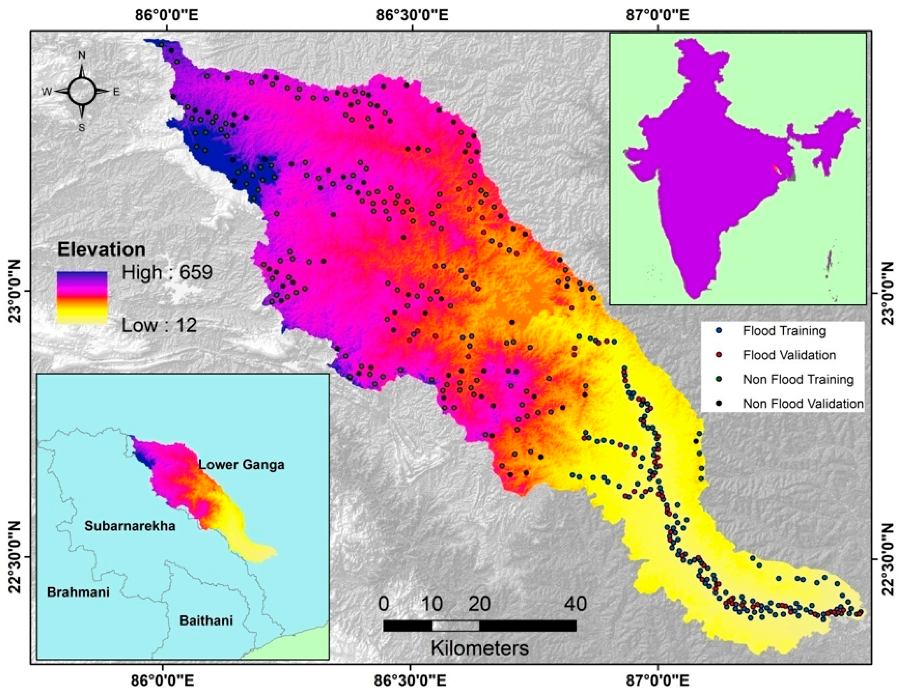
2.1. Study Area
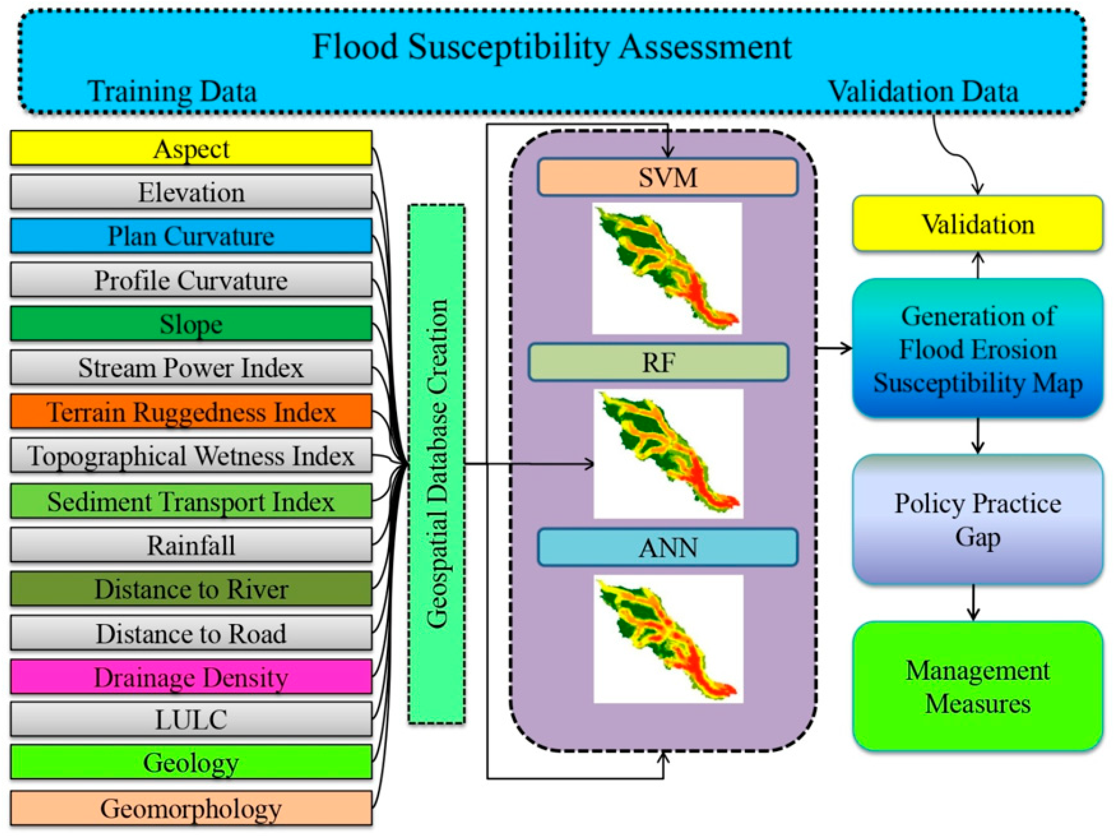
2.2. Methodology
2.3. Flood Inventory Mapping
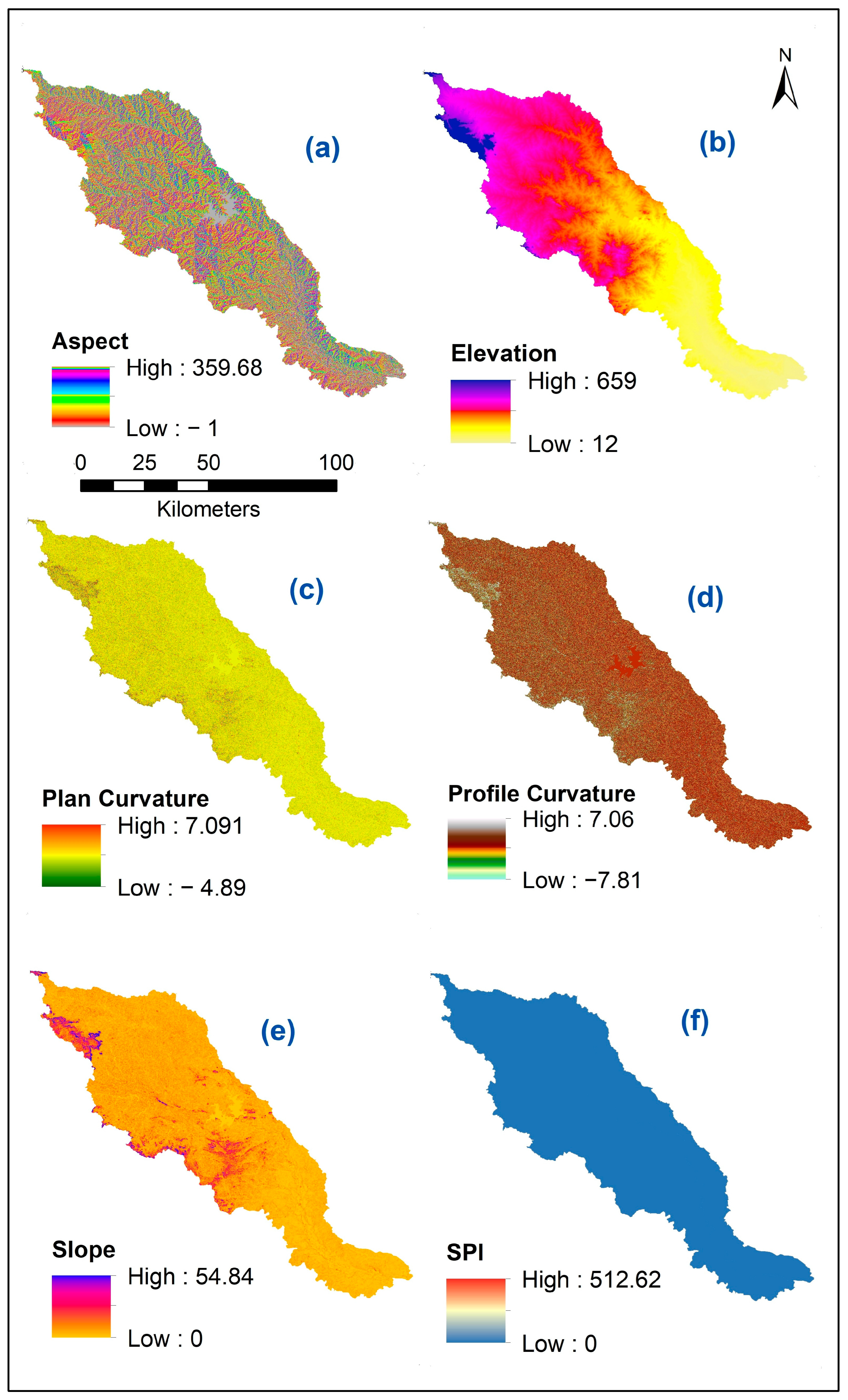
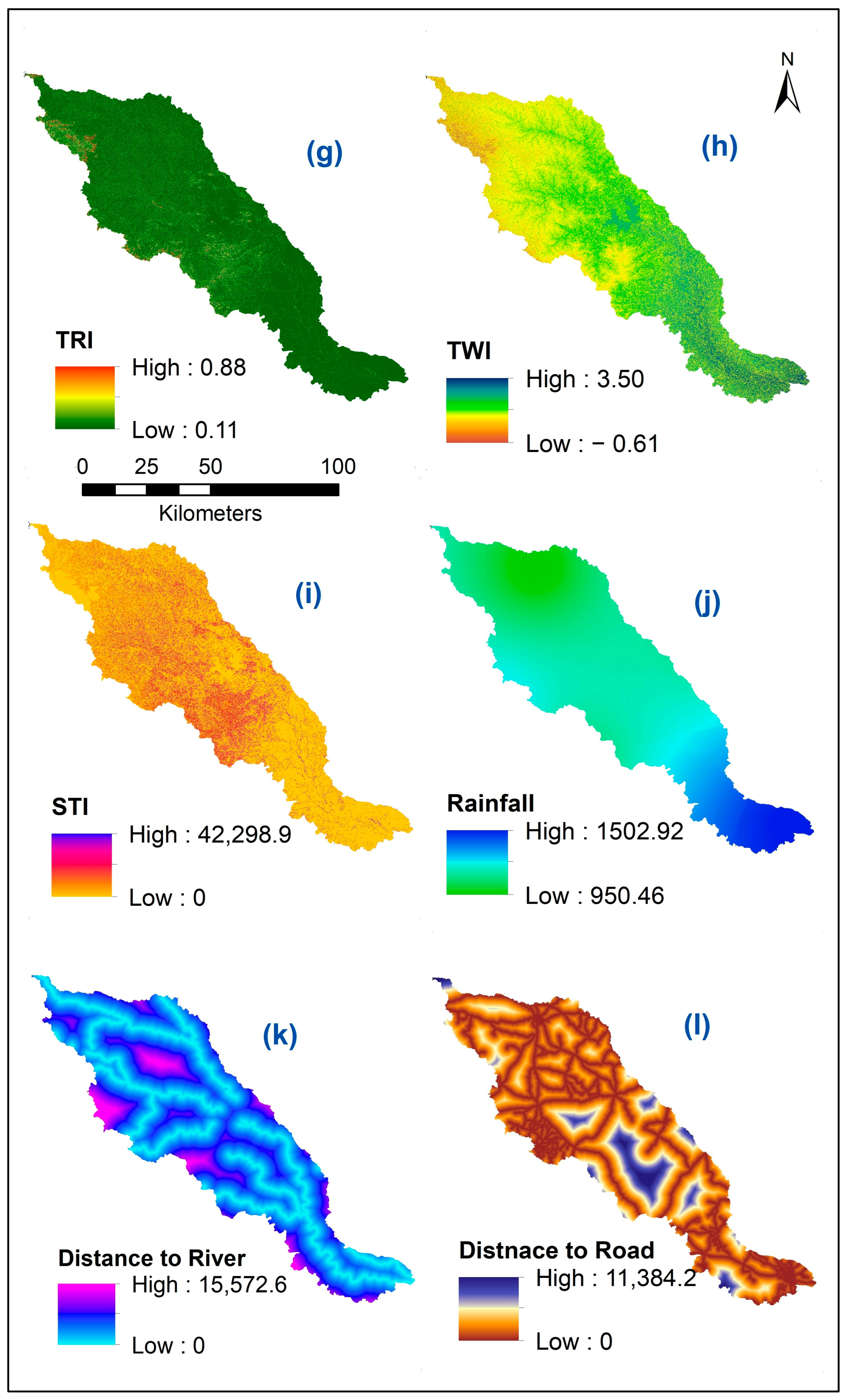
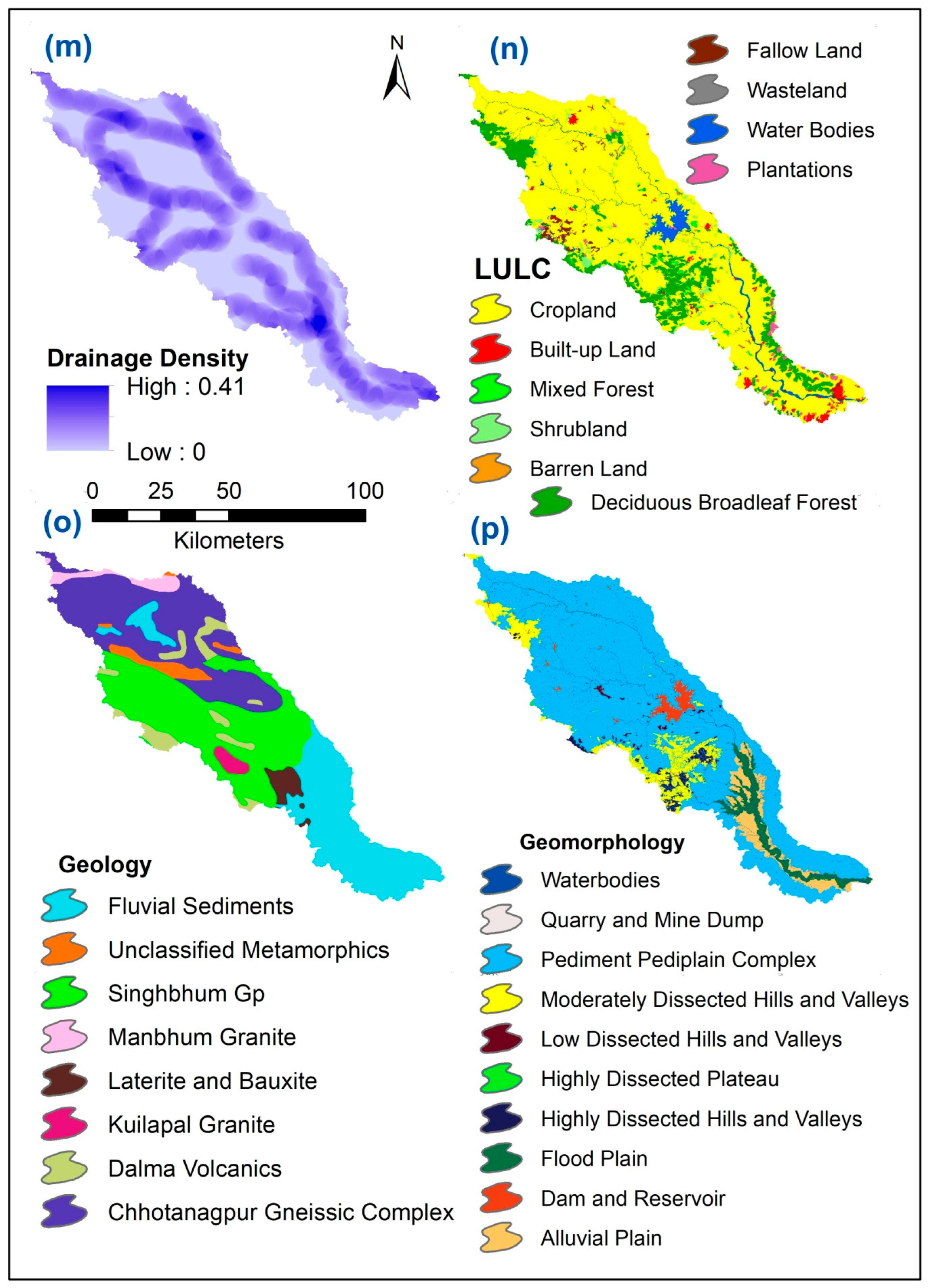
2.4. Causatives Parameter to Flood
2.5. Methods
2.5.1. Multicollinearity Assessment
2.5.2. Random Forest (RF)
2.5.3. Support Vector Machine (SVM)
2.5.4. Artificial Neural Network (ANN)
2.5.5. Model Validation Techniques
3. Results
3.1. Multicollinearity Assessment
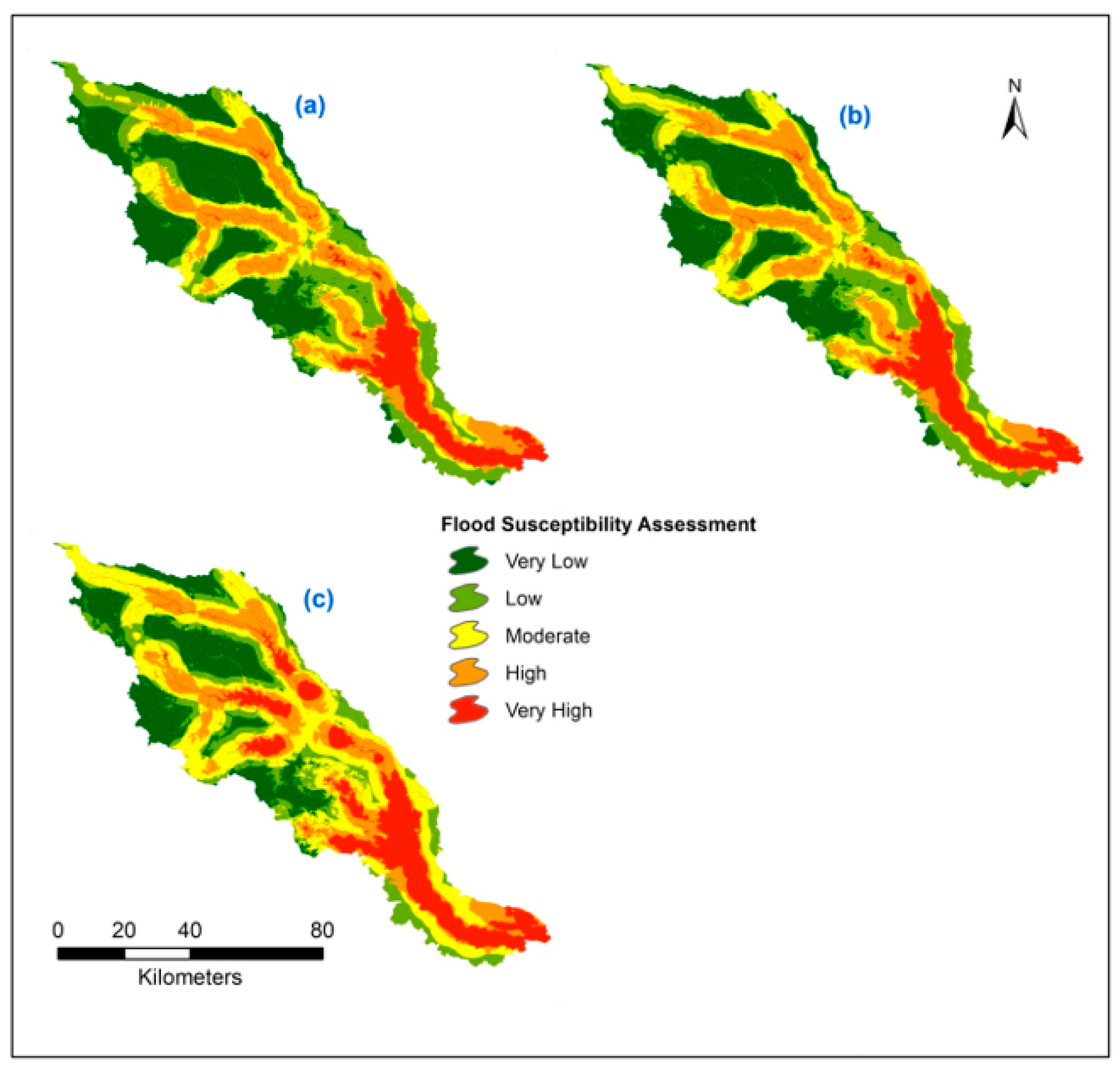
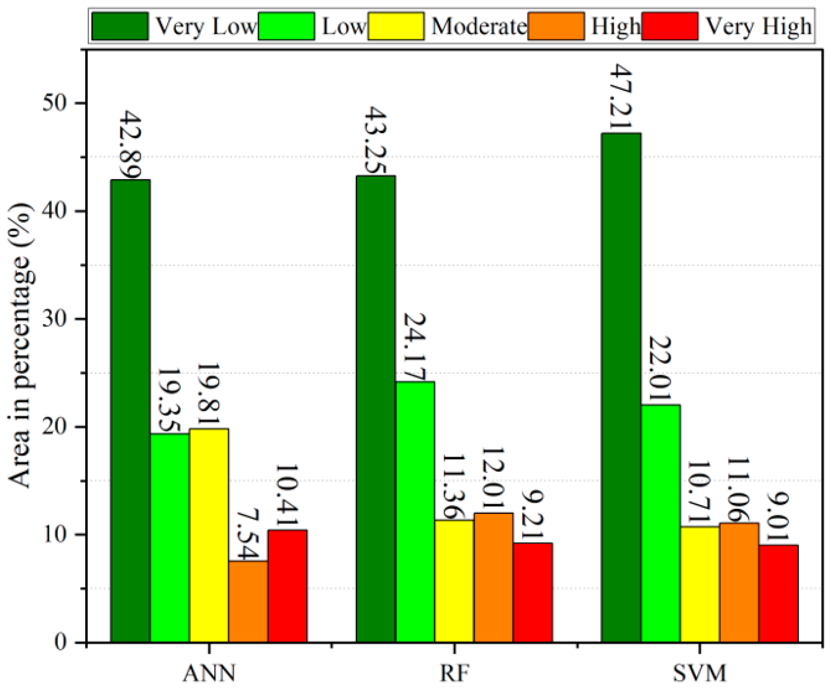
3.2. Flood Susceptibility Assessment
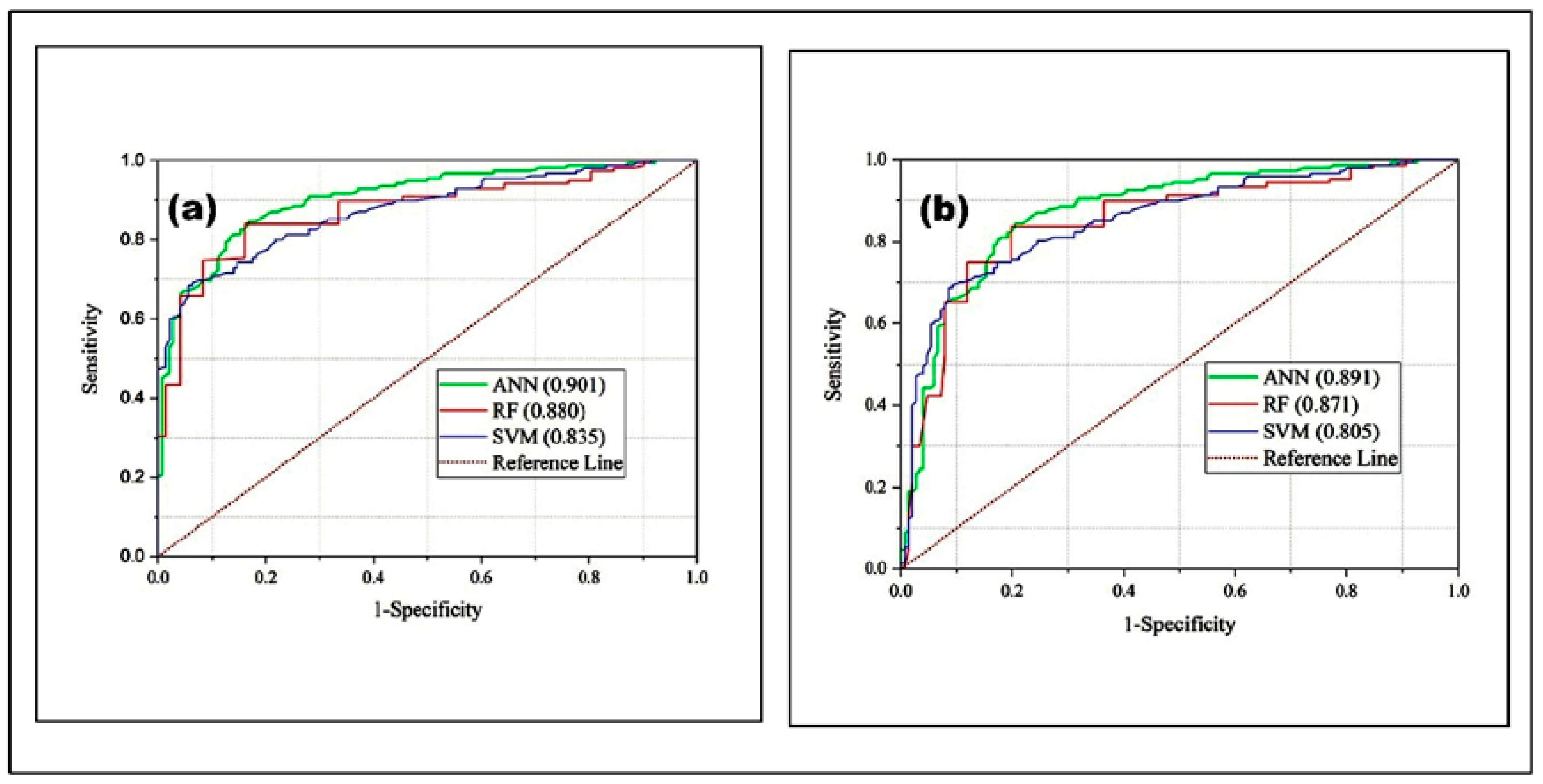
3.3. Model Evaluation
4. Discussion
5. Conclusions
Author Contributions
Funding
Institutional Review Board Statement
Informed Consent Statement
Data Availability Statement
Conflicts of Interest
References
- Lorenzo-Lacruz, J.; Amengual, A.; Garcia, C.; Morán-Tejeda, E.; Homar, V.; Maimó-Far, A.; Hermoso, A.; Ramis, C.; Romero, R. Hydro-Meteorological Reconstruction and Geomorphological Impact Assessment of the October 2018 Catastrophic Flash Flood at Sant Llorenç, Mallorca (Spain). Nat. Hazards Earth Syst. Sci. 2019, 19, 2597–2617. [Google Scholar] [CrossRef] [Green Version]
- Anshuka, A.; van Ogtrop, F.F.; Sanderson, D.; Thomas, E.; Neef, A. Vulnerabilities Shape Risk Perception and Influence Adaptive Strategies to Hydro-Meteorological Hazards: A Case Study of Indo-Fijian Farming Communities. Int. J. Disaster Risk Reduct. 2021, 62, 102401. [Google Scholar] [CrossRef]
- Pratap, S.; Srivastava, P.K.; Routray, A.; Islam, T.; Mall, R.K. Appraisal of Hydro-Meteorological Factors during Extreme Precipitation Event: Case Study of Kedarnath Cloudburst, Uttarakhand, India. Nat. Hazards 2020, 100, 635–654. [Google Scholar] [CrossRef]
- Wahlstrom, M.; Guha-Sapir, D. The Human Cost of Weather-Related Disasters 1995–2015; UNISDR: Geneva, Switzerland, 2015. [Google Scholar]
- Nicholls, R.J.; Hoozemans, F.M.; Marchand, M. Increasing Flood Risk and Wetland Losses Due to Global Sea-Level Rise: Regional and Global Analyses. Glob. Environ. Chang. 1999, 9, S69–S87. [Google Scholar] [CrossRef]
- Liu, S.; Huang, S.; Xie, Y.; Wang, H.; Leng, G.; Huang, Q.; Wei, X.; Wang, L. Identification of the Non-Stationarity of Floods: Changing Patterns, Causes, and Implications. Water Resour. Manag. 2019, 33, 939–953. [Google Scholar] [CrossRef]
- Manzoor, Z.; Ehsan, M.; Khan, M.B.; Manzoor, A.; Akhter, M.M.; Sohail, M.T.; Hussain, A.; Shafi, A.; Abu-Alam, T.; Abioui, M. Floods and Flood Management and Its Socio-Economic Impact on Pakistan: A Review of the Empirical Literature. Front. Environ. Sci. 2022, 10, 2480. [Google Scholar] [CrossRef]
- Sohail, M.T.; Hussan, A.; Ehsan, M.; Al-Ansari, N.; Akhter, M.M.; Manzoor, Z.; Elbeltagi, A. Groundwater Budgeting of Nari and Gaj Formations and Groundwater Mapping of Karachi, Pakistan. Appl. Water Sci. 2022, 12, 267. [Google Scholar] [CrossRef]
- Tralli, D.M.; Blom, R.G.; Zlotnicki, V.; Donnellan, A.; Evans, D.L. Satellite Remote Sensing of Earthquake, Volcano, Flood, Landslide and Coastal Inundation Hazards. ISPRS J. Photogramm. Remote Sens. 2005, 59, 185–198. [Google Scholar] [CrossRef]
- Ran, J.; Nedovic-Budic, Z. Integrating Spatial Planning and Flood Risk Management: A New Conceptual Framework for the Spatially Integrated Policy Infrastructure. Comput. Environ. Urban Syst. 2016, 57, 68–79. [Google Scholar] [CrossRef] [Green Version]
- Li, X.; Yan, D.; Wang, K.; Weng, B.; Qin, T.; Liu, S. Flood Risk Assessment of Global Watersheds Based on Multiple Machine Learning Models. Water 2019, 11, 1654. [Google Scholar] [CrossRef] [Green Version]
- Stefanidis, S.; Alexandridis, V.; Theodoridou, T. Flood Exposure of Residential Areas and Infrastructure in Greece. Hydrology 2022, 9, 145. [Google Scholar] [CrossRef]
- Qiang, Y. Flood Exposure of Critical Infrastructures in the United States. Int. J. Disaster Risk Reduct. 2019, 39, 101240. [Google Scholar] [CrossRef]
- Hapuarachchi, H.; Wang, Q.; Pagano, T. A Review of Advances in Flash Flood Forecasting. Hydrol. Process. 2011, 25, 2771–2784. [Google Scholar] [CrossRef]
- Li, D.; Marshall, L.; Liang, Z.; Sharma, A.; Zhou, Y. Characterizing Distributed Hydrological Model Residual Errors Using a Probabilistic Long Short-Term Memory Network. J. Hydrol. 2021, 603, 126888. [Google Scholar] [CrossRef]
- Pradhan, A.; Indu, J. Uncertainty in Calibration of Variable Infiltration Capacity Model. In Hydrology in a Changing World: Challenges in Modeling; Singh, S.K., Dhanya, C.T., Eds.; Springer Water; Springer International Publishing: Cham, Switzerland, 2019; pp. 89–108. ISBN 978-3-030-02197-9. [Google Scholar]
- Chapi, K.; Singh, V.P.; Shirzadi, A.; Shahabi, H.; Bui, D.T.; Pham, B.T.; Khosravi, K. A Novel Hybrid Artificial Intelligence Approach for Flood Susceptibility Assessment. Environ. Model. Softw. 2017, 95, 229–245. [Google Scholar] [CrossRef]
- Khosravi, K.; Shahabi, H.; Pham, B.T.; Adamowski, J.; Shirzadi, A.; Pradhan, B.; Dou, J.; Ly, H.-B.; Gróf, G.; Ho, H.L. A Comparative Assessment of Flood Susceptibility Modeling Using Multi-Criteria Decision-Making Analysis and Machine Learning Methods. J. Hydrol. 2019, 573, 311–323. [Google Scholar] [CrossRef]
- Roy, P.; Chandra Pal, S.; Chakrabortty, R.; Chowdhuri, I.; Malik, S.; Das, B. Threats of Climate and Land Use Change on Future Flood Susceptibility. J. Clean. Prod. 2020, 272, 122757. [Google Scholar] [CrossRef]
- Nachappa, T.G.; Piralilou, S.T.; Gholamnia, K.; Ghorbanzadeh, O.; Rahmati, O.; Blaschke, T. Flood Susceptibility Mapping with Machine Learning, Multi-Criteria Decision Analysis and Ensemble Using Dempster Shafer Theory. J. Hydrol. 2020, 590, 125275. [Google Scholar] [CrossRef]
- Alkhodari, M.; Jelinek, H.F.; Saleem, S.; Hadjileontiadis, L.J.; Khandoker, A.H. Revisiting Left Ventricular Ejection Fraction Levels: A Circadian Heart Rate Variability-Based Approach. IEEE Access 2021, 9, 130111–130126. [Google Scholar] [CrossRef]
- Bui, D.T.; Pradhan, B.; Lofman, O.; Revhaug, I.; Dick, O.B. Landslide Susceptibility Mapping at HoaBinh Province (Vietnam) Using an Adaptive Neuro-Fuzzy Inference System and GIS. Comput. Geosci. 2012, 45, 199–211. [Google Scholar]
- Islam, A.R.M.T.; Talukdar, S.; Mahato, S.; Kundu, S.; Eibek, K.U.; Pham, Q.B.; Kuriqi, A.; Linh, N.T.T. Flood Susceptibility Modelling Using Advanced Ensemble Machine Learning Models. Geosci. Front. 2021, 12, 101075. [Google Scholar] [CrossRef]
- Zhao, G.; Pang, B.; Xu, Z.; Yue, J.; Tu, T. Mapping Flood Susceptibility in Mountainous Areas on a National Scale in China. Sci. Total Environ. 2018, 615, 1133–1142. [Google Scholar] [CrossRef] [PubMed]
- Costache, R.; Arabameri, A.; Elkhrachy, I.; Ghorbanzadeh, O.; Pham, Q.B. Detection of Areas Prone to Flood Risk Using State-of-the-Art Machine Learning Models. Geomat. Nat. Hazards Risk 2021, 12, 1488–1507. [Google Scholar] [CrossRef]
- Saha, T.K.; Pal, S.; Talukdar, S.; Debanshi, S.; Khatun, R.; Singha, P.; Mandal, I. How Far Spatial Resolution Affects the Ensemble Machine Learning Based Flood Susceptibility Prediction in Data Sparse Region. J. Environ. Manag. 2021, 297, 113344. [Google Scholar] [CrossRef] [PubMed]
- Liu, Y.; De Smedt, F. Flood Modeling for Complex Terrain Using GIS and Remote Sensed Information. Water Resour. Manag. 2005, 19, 605–624. [Google Scholar] [CrossRef]
- Kia, M.B.; Pirasteh, S.; Pradhan, B.; Mahmud, A.R.; Sulaiman, W.N.A.; Moradi, A. An Artificial Neural Network Model for Flood Simulation Using GIS: Johor River Basin, Malaysia. Environ. Earth Sci. 2012, 67, 251–264. [Google Scholar] [CrossRef]
- Tehrany, M.S.; Pradhan, B.; Mansor, S.; Ahmad, N. Flood Susceptibility Assessment Using GIS-Based Support Vector Machine Model with Different Kernel Types. Catena 2015, 125, 91–101. [Google Scholar] [CrossRef]
- Rahmati, O.; Pourghasemi, H.R. Identification of Critical Flood Prone Areas in Data-Scarce and Ungauged Regions: A Comparison of Three Data Mining Models. Water Resour. Manag. 2017, 31, 1473–1487. [Google Scholar] [CrossRef]
- Rahmati, O.; Pourghasemi, H.R.; Zeinivand, H. Flood Susceptibility Mapping Using Frequency Ratio and Weights-of-Evidence Models in the Golastan Province, Iran. Geocarto Int. 2016, 31, 42–70. [Google Scholar] [CrossRef]
- Siahkamari, S.; Haghizadeh, A.; Zeinivand, H.; Tahmasebipour, N.; Rahmati, O. Spatial Prediction of Flood-Susceptible Areas Using Frequency Ratio and Maximum Entropy Models. Geocarto Int. 2018, 33, 927–941. [Google Scholar] [CrossRef]
- Fernández, D.; Lutz, M.A. Urban Flood Hazard Zoning in Tucumán Province, Argentina, Using GIS and Multicriteria Decision Analysis. Eng. Geol. 2010, 111, 90–98. [Google Scholar] [CrossRef]
- Youssef, A.M.; Pradhan, B.; Sefry, S.A. Flash Flood Susceptibility Assessment in Jeddah City (Kingdom of Saudi Arabia) Using Bivariate and Multivariate Statistical Models. Environ. Earth Sci. 2015, 75, 12. [Google Scholar] [CrossRef]
- Tehrany, M.S.; Jones, S.; Shabani, F. Identifying the Essential Flood Conditioning Factors for Flood Prone Area Mapping Using Machine Learning Techniques. Catena 2019, 175, 174–192. [Google Scholar] [CrossRef]
- Lacombe, G.; Valentin, C.; Sounyafong, P.; De Rouw, A.; Soulileuth, B.; Silvera, N.; Pierret, A.; Sengtaheuanghoung, O.; Ribolzi, O. Linking Crop Structure, Throughfall, Soil Surface Conditions, Runoff and Soil Detachment: 10 Land Uses Analyzed in Northern Laos. Sci. Total Environ. 2018, 616, 1330–1338. [Google Scholar] [CrossRef]
- Pallard, B.; Castellarin, A.; Montanari, A. A Look at the Links between Drainage Density and Flood Statistics. Hydrol. Earth Syst. Sci. 2009, 13, 1019–1029. [Google Scholar] [CrossRef] [Green Version]
- Bhagwat, T.N.; Shetty, A.; Hegde, V. Spatial Variation in Drainage Characteristics and Geomorphic Instantaneous Unit Hydrograph (GIUH); Implications for Watershed Management—A Case Study of the Varada River Basin, Northern Karnataka. Catena 2011, 87, 52–59. [Google Scholar] [CrossRef]
- Saha, A.; Pal, S.C.; Arabameri, A.; Blaschke, T.; Panahi, S.; Chowdhuri, I.; Chakrabortty, R.; Costache, R.; Arora, A. Flood Susceptibility Assessment Using Novel Ensemble of Hyperpipes and Support Vector Regression Algorithms. Water 2021, 13, 241. [Google Scholar] [CrossRef]
- Ruidas, D.; Pal, S.C.; Saha, A.; Chowdhuri, I.; Shit, M. Hydrogeochemical Characterization Based Water Resources Vulnerability Assessment in India’s First Ramsar Site of Chilka Lake. Mar. Pollut. Bull. 2022, 184, 114107. [Google Scholar] [CrossRef]
- Malik, S.; Pal, S.C.; Arabameri, A.; Chowdhuri, I.; Saha, A.; Chakrabortty, R.; Roy, P.; Das, B. GIS-Based Statistical Model for the Prediction of Flood Hazard Susceptibility. Environ. Dev. Sustain. 2021, 23, 16713–16743. [Google Scholar] [CrossRef]
- Band, S.S.; Janizadeh, S.; Chandra Pal, S.; Saha, A.; Chakrabortty, R.; Melesse, A.M.; Mosavi, A. Flash Flood Susceptibility Modeling Using New Approaches of Hybrid and Ensemble Tree-Based Machine Learning Algorithms. Remote Sens. 2020, 12, 3568. [Google Scholar] [CrossRef]
- Ahmad, M.W.; Reynolds, J.; Rezgui, Y. Predictive Modelling for Solar Thermal Energy Systems: A Comparison of Support Vector Regression, Random Forest, Extra Trees and Regression Trees. J. Clean. Prod. 2018, 203, 810–821. [Google Scholar] [CrossRef]
- Fawagreh, K.; Gaber, M.M.; Elyan, E. Random Forests: From Early Developments to Recent Advancements. Syst. Sci. Control Eng. Open Access J. 2014, 2, 602–609. [Google Scholar] [CrossRef] [Green Version]
- Sun, J.; Lang, J.; Fujita, H.; Li, H. Imbalanced Enterprise Credit Evaluation with DTE-SBD: Decision Tree Ensemble Based on SMOTE and Bagging with Differentiated Sampling Rates. Inf. Sci. 2018, 425, 76–91. [Google Scholar] [CrossRef]
- Loh, W. Classification and Regression Trees. Wiley Interdiscip. Rev. Data Min. Knowl. Discov. 2011, 1, 14–23. [Google Scholar] [CrossRef]
- Breiman, L. Random Forests. Mach. Learn. 2001, 45, 5–32. [Google Scholar] [CrossRef] [Green Version]
- Tien Bui, D.; Pradhan, B.; Lofman, O.; Revhaug, I. Landslide Susceptibility Assessment in Vietnam Using Support Vector Machines, Decision Tree, and Naive Bayes Models. Math. Probl. Eng. 2012, 2012, 974638. [Google Scholar] [CrossRef] [Green Version]
- Jebur, M.N.; Pradhan, B.; Tehrany, M.S. Manifestation of LiDAR-Derived Parameters in the Spatial Prediction of Landslides Using Novel Ensemble Evidential Belief Functions and Support Vector Machine Models in GIS. IEEE J. Sel. Top. Appl. Earth Obs. Remote Sens. 2014, 8, 674–690. [Google Scholar] [CrossRef]
- Marjanović, M.; Kovačević, M.; Bajat, B.; Voženílek, V. Landslide Susceptibility Assessment Using SVM Machine Learning Algorithm. Eng. Geol. 2011, 123, 225–234. [Google Scholar] [CrossRef]
- Luk, K.C.; Ball, J.E.; Sharma, A. An Application of Artificial Neural Networks for Rainfall Forecasting. Math. Comput. Model. 2001, 33, 683–693. [Google Scholar] [CrossRef]
- Kim, D.H.; Kim, Y.J.; Hur, D.S. Artificial Neural Network Based Breakwater Damage Estimation Considering Tidal Level Variation. Ocean. Eng. 2014, 87, 185–190. [Google Scholar] [CrossRef]
- Akmeliawati, R.; Ooi, M.P.-L.; Kuang, Y.C. Real-Time Malaysian Sign Language Translation Using Colour Segmentation and Neural Network. In Proceedings of the 2007 IEEE Instrumentation & Measurement Technology Conference IMTC 2007, Warsaw, Poland, 1–3 May 2007; pp. 1–6. [Google Scholar]
- Chakraborty, K.; Mehrotra, K.; Mohan, C.K.; Ranka, S. Forecasting the Behavior of Multivariate Time Series Using Neural Networks. Neural Netw. 1992, 5, 961–970. [Google Scholar] [CrossRef] [Green Version]
- Daliakopoulos, I.N.; Coulibaly, P.; Tsanis, I.K. Groundwater Level Forecasting Using Artificial Neural Networks. J. Hydrol. 2005, 309, 229–240. [Google Scholar] [CrossRef]
- Ruidas, D.; Pal, S.C.; Islam, A.R.M.T.; Saha, A. Characterization of Groundwater Potential Zones in Water-Scarce Hardrock Regions Using Data Driven Model. Environ. Earth Sci. 2021, 80, 809. [Google Scholar] [CrossRef]
- Ruidas, D.; Pal, S.C.; Towfiqul Islam, A.R.M.; Saha, A. Hydrogeochemical Evaluation of Groundwater Aquifers and Associated Health Hazard Risk Mapping Using Ensemble Data Driven Model in a Water Scares Plateau Region of Eastern India. Expo. Health 2022. [Google Scholar] [CrossRef]
- Taylor, K.E. Summarizing Multiple Aspects of Model Performance in a Single Diagram. J. Geophys. Res. Atmos. 2001, 106, 7183–7192. [Google Scholar] [CrossRef]
- Pal, S.C.; Ruidas, D.; Saha, A.; Islam, A.R.M.T.; Chowdhuri, I. Application of Novel Data-Mining Technique Based Nitrate Concentration Susceptibility Prediction Approach for Coastal Aquifers in India. J. Clean. Prod. 2022, 346, 131205. [Google Scholar] [CrossRef]
- Parida, Y. Economic Impact of Floods in the Indian States. Environ. Dev. Econ. 2020, 25, 267–290. [Google Scholar] [CrossRef]
- Dixit, A. Floods and Vulnerability: Need to Rethink Flood Management. Flood Probl. Manag. South Asia 2003, 28, 155–179. [Google Scholar]
- Singh, O.; Kumar, M. Flood Events, Fatalities and Damages in India from 1978 to 2006. Nat. Hazards 2013, 69, 1815–1834. [Google Scholar] [CrossRef]
- Rahmati, O.; Zeinivand, H.; Besharat, M. Flood Hazard Zoning in Yasooj Region, Iran, Using GIS and Multi-Criteria Decision Analysis. Geomat. Nat. Hazards Risk 2016, 7, 1000–1017. [Google Scholar] [CrossRef] [Green Version]
- Arora, A.; Arabameri, A.; Pandey, M.; Siddiqui, M.A.; Shukla, U.K.; Bui, D.T.; Mishra, V.N.; Bhardwaj, A. Optimization of State-of-the-Art Fuzzy-Metaheuristic ANFIS-Based Machine Learning Models for Flood Susceptibility Prediction Mapping in the Middle Ganga Plain, India. Sci. Total Environ. 2021, 750, 141565. [Google Scholar] [CrossRef] [PubMed]
- Jahangir, M.H.; Mousavi Reineh, S.M.; Abolghasemi, M. Spatial Predication of Flood Zonation Mapping in Kan River Basin, Iran, Using Artificial Neural Network Algorithm. Weather. Clim. Extrem. 2019, 25, 100215. [Google Scholar] [CrossRef]
- Ramesh, V.; Iqbal, S.S. Urban Flood Susceptibility Zonation Mapping Using Evidential Belief Function, Frequency Ratio and Fuzzy Gamma Operator Models in GIS: A Case Study of Greater Mumbai, Maharashtra, India. Geocarto Int. 2022, 37, 581–606. [Google Scholar] [CrossRef]
- Avand, M.; Moradi, H.; Lasboyee, M.R. Spatial Modeling of Flood Probability Using Geo-Environmental Variables and Machine Learning Models, Case Study: Tajan Watershed, Iran. Adv. Space Res. 2021, 67, 3169–3186. [Google Scholar] [CrossRef]
- Ghosh, S.; Saha, S.; Bera, B. Flood Susceptibility Zonation Using Advanced Ensemble Machine Learning Models within Himalayan Foreland Basin. Nat. Hazards Res. 2022. [Google Scholar] [CrossRef]
- Liu, Y.; Lu, X.; Yao, Y.; Wang, N.; Guo, Y.; Ji, C.; Xu, J. Mapping the Risk Zoning of Storm Flood Disaster Based on Heterogeneous Data and a Machine Learning Algorithm in Xinjiang, China. J. Flood Risk Manag. 2021, 14, e12671. [Google Scholar] [CrossRef]
- Ruidas, D.; Saha, A.; Islam, A.R.M.T.; Costache, R.; Pal, S.C. Development of Geo-Environmental Factors Controlled Flash Flood Hazard Map for Emergency Relief Operation in Complex Hydro-Geomorphic Environment of Tropical River, India. Environ. Sci. Pollut. Res. 2022. [Google Scholar] [CrossRef] [PubMed]
- Ruidas, D.; Chakrabortty, R.; Islam, A.R.M.T.; Saha, A.; Pal, S.C. A Novel Hybrid of Meta-Optimization Approach for Flash Flood-Susceptibility Assessment in a Monsoon-Dominated Watershed, Eastern India. Environ. Earth Sci. 2022, 81, 145. [Google Scholar] [CrossRef]
- Bazai, N.A.; Cui, P.; Carling, P.A.; Wang, H.; Hassan, J.; Liu, D.; Zhang, G.; Jin, W. Increasing Glacial Lake Outburst Flood Hazard in Response to Surge Glaciers in the Karakoram. Earth-Sci. Rev. 2021, 212, 103432. [Google Scholar] [CrossRef]
- Wu, J.; Liu, H.; Wei, G.; Song, T.; Zhang, C.; Zhou, H. Flash Flood Forecasting Using Support Vector Regression Model in a Small Mountainous Catchment. Water 2019, 11, 1327. [Google Scholar] [CrossRef] [Green Version]
- Xiong, J.; Li, J.; Cheng, W.; Wang, N.; Guo, L. A GIS-Based Support Vector Machine Model for Flash Flood Vulnerability Assessment and Mapping in China. ISPRS Int. J. Geo-Inf. 2019, 8, 297. [Google Scholar] [CrossRef] [Green Version]
- Avand, M.; Janizadeh, S.; Naghibi, S.A.; Pourghasemi, H.R.; KhosrobeigiBozchaloei, S.; Blaschke, T. A Comparative Assessment of Random Forest and K-Nearest Neighbor Classifiers for Gully Erosion Susceptibility Mapping. Water 2019, 11, 2076. [Google Scholar] [CrossRef] [Green Version]
- Esfandiari, M.; Abdi, G.; Jabari, S.; McGrath, H.; Coleman, D. Flood Hazard Risk Mapping Using a Pseudo Supervised Random Forest. Remote Sens. 2020, 12, 3206. [Google Scholar] [CrossRef]
- Farhadi, H.; Najafzadeh, M. Flood Risk Mapping by Remote Sensing Data and Random Forest Technique. Water 2021, 13, 3115. [Google Scholar] [CrossRef]
- Tian, Y.; Xu, C.; Hong, H.; Zhou, Q.; Wang, D. Mapping Earthquake-Triggered Landslide Susceptibility by Use of Artificial Neural Network (ANN) Models: An Example of the 2013 Minxian (China) Mw 5.9 Event. Geomat. Nat. Hazards Risk 2019, 10, 1–25. [Google Scholar] [CrossRef] [Green Version]
- Andaryani, S.; Nourani, V.; Haghighi, A.T.; Keesstra, S. Integration of Hard and Soft Supervised Machine Learning for Flood Susceptibility Mapping. J. Environ. Manag. 2021, 291, 112731. [Google Scholar] [CrossRef]
- Kawabata, D.; Bandibas, J. Landslide Susceptibility Mapping Using Geological Data, a DEM from ASTER Images and an Artificial Neural Network (ANN). Geomorphology 2009, 113, 97–109. [Google Scholar] [CrossRef]
- Chakrabortty, R.; Chandra Pal, S.; Rezaie, F.; Arabameri, A.; Lee, S.; Roy, P.; Saha, A.; Chowdhuri, I.; Moayedi, H. Flash-Flood Hazard Susceptibility Mapping in Kangsabati River Basin, India. Geocarto Int. 2022, 37, 6713–6735. [Google Scholar] [CrossRef]
- Dano, U.L.; Balogun, A.-L.; Matori, A.-N.; Wan Yusouf, K.; Abubakar, I.R.; Said Mohamed, M.A.; Aina, Y.A.; Pradhan, B. Flood Susceptibility Mapping Using GIS-Based Analytic Network Process: A Case Study of Perlis, Malaysia. Water 2019, 11, 615. [Google Scholar] [CrossRef] [Green Version]
- Falah, F.; Rahmati, O.; Rostami, M.; Ahmadisharaf, E.; Daliakopoulos, I.N.; Pourghasemi, H.R. 14-Artificial Neural Networks for Flood Susceptibility Mapping in Data-Scarce Urban Areas. In Spatial Modeling in GIS and R for Earth and Environmental Sciences; Pourghasemi, H.R., Gokceoglu, C., Eds.; Elsevier: Amsterdam, The Netherlands, 2019; pp. 323–336. ISBN 978-0-12-815226-3. [Google Scholar]
- Shafizadeh-Moghadam, H.; Valavi, R.; Shahabi, H.; Chapi, K.; Shirzadi, A. Novel Forecasting Approaches Using Combination of Machine Learning and Statistical Models for Flood Susceptibility Mapping. J. Environ. Manag. 2018, 217, 1–11. [Google Scholar] [CrossRef] [Green Version]
- Khosravi, K.; Pham, B.T.; Chapi, K.; Shirzadi, A.; Shahabi, H.; Revhaug, I.; Prakash, I.; Tien Bui, D. A Comparative Assessment of Decision Trees Algorithms for Flash Flood Susceptibility Modeling at Haraz Watershed, Northern Iran. Sci. Total Environ. 2018, 627, 744–755. [Google Scholar] [CrossRef] [PubMed]
- Luu, C.; Pham, B.T.; Phong, T.V.; Costache, R.; Nguyen, H.D.; Amiri, M.; Bui, Q.D.; Nguyen, L.T.; Le, H.V.; Prakash, I.; et al. GIS-Based Ensemble Computational Models for Flood Susceptibility Prediction in the Quang Binh Province, Vietnam. J. Hydrol. 2021, 599, 126500. [Google Scholar] [CrossRef]
- Dahri, N.; Yousfi, R.; Bouamrane, A.; Abida, H.; Pham, Q.B.; Derdous, O. Comparison of Analytic Network Process and Artificial Neural Network Models for Flash Flood Susceptibility Assessment. J. Afr. Earth Sci. 2022, 193, 104576. [Google Scholar] [CrossRef]
- Samantaray, S.; Das, S.S.; Sahoo, A.; Satapathy, D.P. Evaluating the Application of Metaheuristic Approaches for Flood Simulation Using GIS: A Case Study of Baitarani River Basin, India. Mater. Today Proc. 2022, 61, 452–465. [Google Scholar] [CrossRef]


| Parameters | Multi-Collinearity | |
|---|---|---|
| TOL | VIF | |
| Aspect | 0.89 | 1.12 |
| Elevation | 0.53 | 1.89 |
| Plan curvature | 1.21 | 0.83 |
| Profile curvature | 0.99 | 1.01 |
| Slope | 0.49 | 2.04 |
| SPI | 0.63 | 1.59 |
| TRI | 0.69 | 1.45 |
| TWI | 0.85 | 1.18 |
| STI | 0.77 | 1.30 |
| Rainfall | 0.78 | 1.28 |
| Distance to river | 0.52 | 1.92 |
| Distance to road | 0.87 | 1.15 |
| Drainage density | 0.32 | 3.13 |
| LULC | 0.67 | 1.49 |
| Geology | 0.71 | 1.41 |
| Geomorphology | 0.89 | 1.12 |
| Models | Stage | Parameters | |||||
|---|---|---|---|---|---|---|---|
| Sensitivity | Specificity | PPV | NPV | F Score | AUC | ||
| ANN | Training | 0.93 | 0.86 | 0.85 | 0.90 | 0.89 | 0.901 |
| Validation | 0.92 | 0.85 | 0.85 | 0.91 | 0.88 | 0.891 | |
| RF | Training | 0.92 | 0.87 | 0.91 | 0.91 | 0.89 | 0.880 |
| Validation | 0.91 | 0.82 | 0.93 | 0.92 | 0.86 | 0.871 | |
| SVM | Training | 0.91 | 0.86 | 0.89 | 0.95 | 0.88 | 0.835 |
| Validation | 0.89 | 0.83 | 0.86 | 0.97 | 0.86 | 0.805 | |
Disclaimer/Publisher’s Note: The statements, opinions and data contained in all publications are solely those of the individual author(s) and contributor(s) and not of MDPI and/or the editor(s). MDPI and/or the editor(s) disclaim responsibility for any injury to people or property resulting from any ideas, methods, instructions or products referred to in the content. |
© 2023 by the authors. Licensee MDPI, Basel, Switzerland. This article is an open access article distributed under the terms and conditions of the Creative Commons Attribution (CC BY) license (https://creativecommons.org/licenses/by/4.0/).
Share and Cite
Chakrabortty, R.; Pal, S.C.; Ruidas, D.; Roy, P.; Saha, A.; Chowdhuri, I. Living with Floods Using State-of-the-Art and Geospatial Techniques: Flood Mitigation Alternatives, Management Measures, and Policy Recommendations. Water 2023, 15, 558. https://doi.org/10.3390/w15030558
Chakrabortty R, Pal SC, Ruidas D, Roy P, Saha A, Chowdhuri I. Living with Floods Using State-of-the-Art and Geospatial Techniques: Flood Mitigation Alternatives, Management Measures, and Policy Recommendations. Water. 2023; 15(3):558. https://doi.org/10.3390/w15030558
Chicago/Turabian StyleChakrabortty, Rabin, Subodh Chandra Pal, Dipankar Ruidas, Paramita Roy, Asish Saha, and Indrajit Chowdhuri. 2023. "Living with Floods Using State-of-the-Art and Geospatial Techniques: Flood Mitigation Alternatives, Management Measures, and Policy Recommendations" Water 15, no. 3: 558. https://doi.org/10.3390/w15030558