
Analysis of Optimal Sensor Placement in Looped Water Distribution Networks Using Different Water Quality Models


School of Engineering and Architecture, University of Enna “Kore”, Cittadella Universitaria, 94100 Enna, Italy
*
Author to whom correspondence should be addressed.
Water 2023, 15(3), 559; https://doi.org/10.3390/w15030559
Submission received: 28 December 2022
/
Revised: 16 January 2023
/
Accepted: 27 January 2023
/
Published: 31 January 2023
(This article belongs to the Special Issue Urban Water Networks Modelling and Monitoring, Volume II)
Abstract
:Urban looped water distribution systems are highly vulnerable to water quality issues. They could be subject to contamination events (accidental or deliberate), compromising the water quality inside them and causing damage to the users’ health. An efficient monitoring system must be developed to prevent this, supported by a suitable model for assessing water quality. Currently, several studies use advective–reactive models to analyse water quality, neglecting diffusive transport, which is claimed to be irrelevant in turbulent flows. Although this may be true in simple systems, such as linear transport pipes, the presence of laminar flows in looped systems may be significant, especially at night and in the peripheral parts of the network. In this paper, a numerical optimisation approach has been compared with the results of an experimental campaign using three different numerical models as inputs (EPANET advective model, the AZRED model in which diffusion–dispersion equations have been implemented, and a new diffusive–dispersive model in dynamic conditions using the random walk method, EPANET-DD). The optimisation problem was formulated using the Monte Carlo method. The results demonstrated a significant difference in sensor placement based on the numerical model.
1. Introduction
An emerging problem in recent years concerns the scarcity of water resources, which is linked to the quantity of available water and includes the quality aspect. This results in the need for users to use water of marginal quality. This problem does concern not only the arid (Central America, Africa, and the Arabian Peninsula) and semi-arid areas of the world but also those regions where rainfall is relatively abundant and where urbanisation endangers water quality [1].
This has led to an increased focus on water quality monitoring in urban water systems in recent years [2,3]. Such studies typically integrate monitoring and modelling to obtain a reliable picture of the systems, reducing the costs of real-time monitoring [4].
In a water distribution network (WDN), water quality may be compromised due to the accidental introduction or deliberate release of contaminants, resulting in a public health issue [5,6]. To better identify contamination events, it is essential to determine the optimal position of the probes to minimise equipment costs [7] and maximise detection efficiency [8] while at the same time reducing contamination risks [9].
The choice of a fixed or mobile monitoring system differently affects measurements, as it has been reported that the use of sensors installed within the water supply helps to monitor water more continuously than sampling modes [10,11,12]. Therefore, it is critical to use real-time monitoring systems, although the installation and operating costs are greater than those of a system that uses static control [13].
Furthermore, enormous importance in the optimal positioning of the water quality sensors is assumed by some optimisation criteria that produce an effective monitoring system, such as expected time to detection, the expected population affected, expected contaminated water demand and detection likelihood, which is associated with the different contamination scenarios that can occur within the water distribution network [14].
Current state-of-the-art water distribution system analysis usually adopts a simplified approach to water quality modelling, neglecting dispersion and diffusion and focusing on simplified or detailed reaction kinetics. Ohar et al. (2015) [15] solved the sensor optimisation problem by using the EPANET-MSX (Multi-Species eXtension) model to simulate the contamination of three literature networks (Net3, BWSN 1, and Dover) with three organophosphates that were simulated using detailed contamination kinetics. Furthermore, the authors considered quantitative measures of the population affected by these contaminants because of such intrusions. Yang and Boccelli (2016) [16] used the same modelling approach but incorporated dynamic water quality models to simulate the response of water quality parameters more realistically to a network-scale contamination event. The authors also evaluated current risk assessment assumptions for sensor placement and the performance of event detection algorithms (EDAs). The results demonstrated that current EDA assessment approaches and contamination warning system (CWS) design assumptions might need to be revised to adequately represent the actual evolution of events in a distribution system under common low-flow conditions.
Abokifa et al. (2020) [17] used the EPANET model and the WUDESIM model (advective-dispersive model for a single species) in their development to model the behaviour of chlorine within water networks. However, the authors found a better result in modelling water quality using the complete model, which considers the dispersion process in order not to overestimate the residual chlorine concentrations in dead-end branches and partially mask the deterioration in water quality due to reduced demand.
Numerous studies have highlighted the importance of considering diffusive–dispersive processes in water distribution systems. First, from 1953–1954, Taylor numerically analysed the dispersive phenomenon in laminar and turbulent flow regimes to determine the value of the dispersion coefficient and show how it is related to flow regime quantities [18,19].
Axworthy and Karney (1996) [20] found that dispersive–diffusive transport processes became relevant when the flow velocity was low and when the Reynolds number was less than 50,000, which is common in urban water distribution networks at night. This was demonstrated by combining the limiting velocity and the coefficient dispersion to adjust the dispersion’s sensitivity to the flow velocity at a particular position. After analytical applications, they discovered that dispersive effects tended to disappear as speed increased and became negligible; thus, an advective transport model should be suitable for any analytical need.
Romero-Gomez and Choi (2011) [21] realised that the presence of a solute persists long after a tracer pulse has passed a fixed downstream position and revealed that the dispersion velocity near the end of the pulse is greater than the velocity near the front of the pulse. This result occurs because low-speed regions close to the wall strongly impede solute transport due to the non-slip boundary condition. Such conditions differ for dispersion upstream and downstream of the contaminant injection. For this reason, they specified the dispersion coefficient while considering the effect of flow direction on dispersion. This approach was used in their study because it highlights the difference between mass flows backwards and forwards from a specific position, which results in different dispersion velocities that lead to solute transport in both directions.
Furthermore, the importance of these transport processes has been studied and experimentally validated by Piazza et al. (2020) [22], who observed that their importance decreased in the presence of turbulence in the pipes, which produces a very different result in terms of sensor positioning.
For this reason, this work aims to demonstrate how the positioning of quality sensors changes depending on the numerical model used. Three different numerical models were used to reproduce the experimental data maintaining constant the hydraulic features: an EPANET advective model [23], in which the solute transport mechanisms are relatively simple, of the plug-flow type; the AZRED model in which the diffusion-dispersion equations proposed by Romero-Gomez and Choi (2011) [21] are inserted, and a new diffusive–dispersive model that solves the advection–diffusion equation (ADE) in the two-dimensional case under dynamic conditions EPANET-DD (dynamic dispersion) [24].
2. Materials and Methods
2.1. Experimental Setup and Conditions
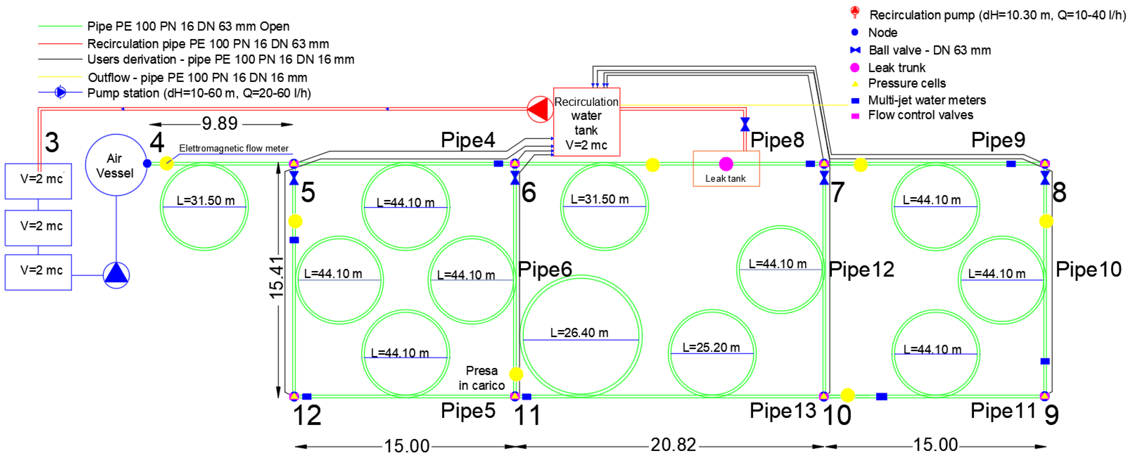
The experimental network of Enna University (UKE) is a closed water distribution network composed of high-density polyethene pipes (HDPE 100) with a nominal pressure of 16 bar (PN16), a DN (nominal diameter) of 63 mm, and a thickness of 5.8 mm. The net is divided into three meshes, each of which contains pipe windings with a radius of 2.0 m and a length of approximately 45 m. Eight “users” are connected to the leading network through eight internal nodes consisting of multilayer polyethene pipes with diameters of 20 mm (internal diameter of 12.7 mm), which simulate the domestic users of a virtual network (Figure 1 and Figure 2).
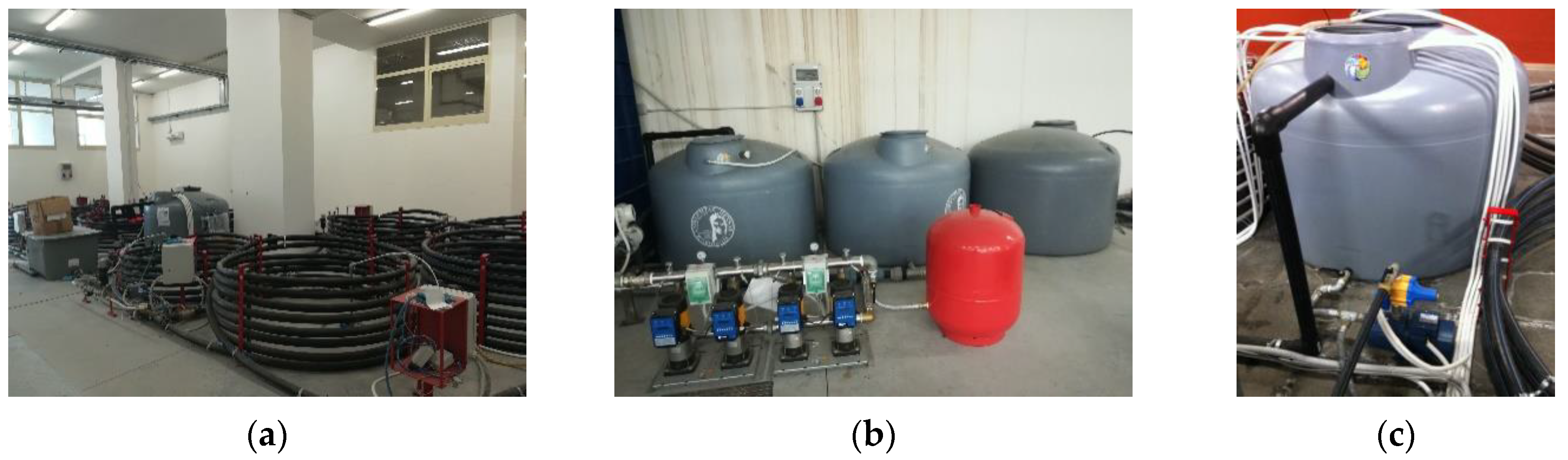
Four polyethene tanks supply the network, three hydraulically connected upstream of the pumping system, and one centrally positioned to the network. The collected flows are conveyed to the user nodes, which feed the other three via a recirculation pump. Overall, the tanks can store up to 8 m3 of water (Figure 2). The pumping system, which consists of four vertical multistage centrifugal electric pumps and an air vessel that allows pressure stabilisation, behaves like a constant load tank, keeping the pressure constant and equal to a pre-set value between 1 and 6 bar with a tolerance of 0.05 bar; the pumping system varies the speed of the pumps.
The system flows in the pipes are monitored by five electromagnetic flow meters installed in various sections of the network (trunks 4–5, 6–7, 7–8, 9–10, and 11–12). In addition, pressure cells and multi-jet water meters are present in each node. Furthermore, Wi-Fi real-time remote-controlled conductivity probes were positioned at each node and connected with the monitoring appliances via a central computer, which was also capable of regulating flows supplied to users via remote-controlled valves. The conductivity probes had an accuracy ranging from 1300 μs to 40,000 μs and outputted the conductivity values in μs, the total dissolved solids (TDS), and the salinity. The salinity values were derived from the practical salinity scale (PSS-78). The real-time Wi-Fi remote control system consisted of a Wi-Fi router with 8 Arduino cards outfitted with conductivity probes. The Arduino cards were programmed with a sample code to detect the desired sizes. All data were collected with the Wi-Fi data acquisition cards and sent to the server. Experiments were carried out by varying the outflows in nodes 6, 7, 8, and 10 (kept constant in each experiment) with flows ranging from 80 L/h to 400 L/h to obtain different flow regimes in the pipes. No leakages were applied in the present study.
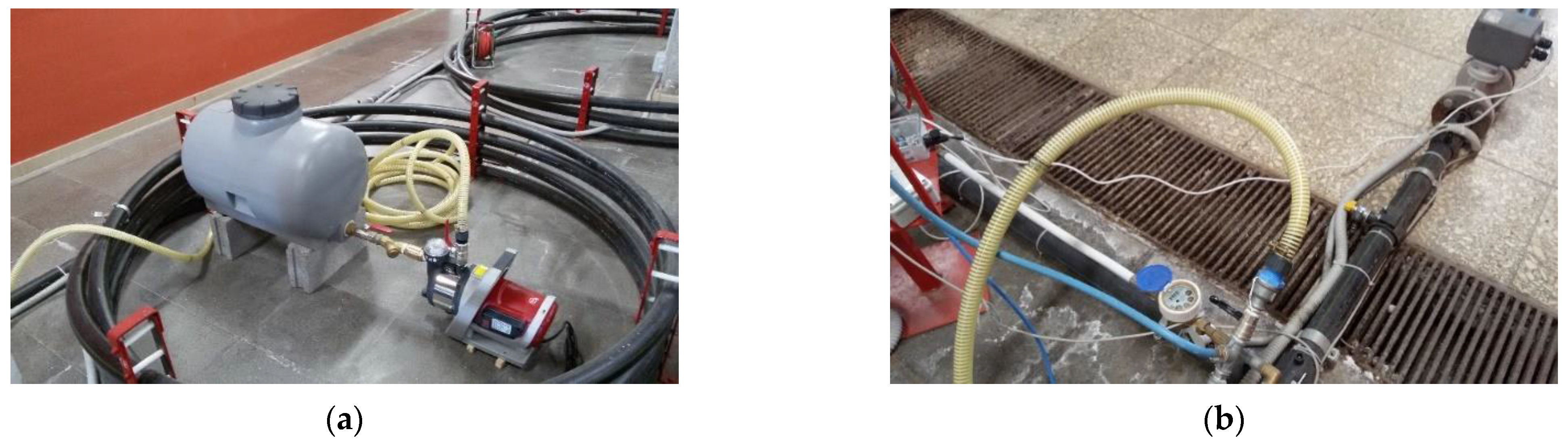
The network was equipped with a 100-litre polyethene tank and an injection pump connected to one of the network nodes chosen at random via a flexible PVC pipe approximately 50 m in length and 40 mm in diameter (Figure 3) to carry out contamination experiments. Sodium chloride was selected as the contaminant because it is easy to find, inexpensive, nontoxic, and easy for probes to detect. The experiments were carried out considering all branches of the network open.
2.2. Optimisation of Sensor Placement
The optimisation problem, i.e., finding the best solution of all feasible solutions, was solved using the Monte Carlo method, which is based on probabilistic procedures and can solve problems presenting analytical difficulties that would otherwise be difficult to overcome [25].
Conceptually, the method is based on the possibility of sampling an assigned probability distribution, F(X), using numbers drawn at random (random numbers); that is, the possibility of generating a sequence of events, X1, X2…, Xn…, is distributed according to F(X). However, instead of using numbers drawn at random, the authors use a sequence of numbers obtained through a well-defined iterative process; these numbers are referred to as pseudorandom because they are not random but possess the statistical properties of random numbers.
The Monte Carlo method yields reliable answers in studying real complex systems. However, the solution obtained is never exact in a statistical sense, as it is subject to uncertainty, which decreases as the number of statistical samples increases.
In the present case, the Monte Carlo method was used to solve the optimisation problem for positioning three water quality sensors within the laboratory network of UKE, which is fully described in the previous section. Given the uncertainty in the position, magnitude, and duration of the contamination, 1000 simulations were performed, with the contamination parameters (mass of contaminant, duration of contamination, and contamination node) set at random. User demands in all nodes were fixed at 2.5 L/min. In addition, the inlet head was fixed to 1.5 bar. At the same time, an experiment was carried out in node 5, with a duration of 3 min and a mass of 460 g (leading to a constant concentration of 4600 mg/L), developing the three flow regimes (Turbulent, Transition, Laminar), See Piazza et al. (2022) [26] for more details.
Three objective functions were used:
- F_1, the detection likelihood, i.e., the probability that a sensor configuration will detect the contamination;
- F_2, the detection time, i.e., the average time between contamination and detection in 200 simulations;
- F_3, the detection redundancy, i.e., the probability that two sensors detect the contamination within 20 min.
The objective functions were slightly modified from those presented in Preis and Ostfeld (2008) [6] to comply with the smaller dimensions of the analysed network. However, they were equally weighted in selecting the optimal sensor location.
The modelling analysis was carried out using the state-of-the-art advective EPANET model, the AZRED model (advective–diffusive–dispersive model), which includes the diffusion and dispersion equations proposed by Romero-Gomez and Choi (2011) [21], and a new diffusive–dispersive model developed by the authors called EPANET-DD (dynamic-dispersion), after an appropriate hydraulic and qualitative calibration [24].
The classic advective EPANET model solves the advective transport equation by solving a mass balance of the fundamental plug-flow substance that accounts for the advective transport and might include kinetic reaction processes (Equation (1)). The substance mass is assigned to discrete volume elements once all the connections in the network have been partitioned using this approach. Next, the concentration within each volume segment is subjected to reactions and transferred to the adjacent downstream segment. If the latter is a junction node, the incoming mass and flow volumes are combined with those already present at the network nodes. Finally, once these processes have been exhausted for all network elements, the concentration is calculated and released in the first pipe segments, with flow leaving the node. In this case, the effect of longitudinal dispersion needs to be addressed, as it is not considered necessary in most operating conditions [26].
In the present application, in which a conservative tracer is used, the reaction term is neglected.
In contrast, the AZRED model, which includes the diffusion and dispersion equations proposed by Romero-Gomez and Choi (2011) [21], solves the transport equation by highlighting the differences between mass flows backwards and forwards from a specific position, which results in different dispersion speeds that lead to solute transport in both directions (Equation (2)).
in which
and
where (Equations (4) and (5)) are the dispersion parameters backwards and forwards with respect to the flow direction, is the average flow velocity, and .
The dimensionless travel time (T) was calculated as in Equation (6). This parameter indicates how far the dispersion coefficient has progressed towards achieving stable conditions.
in which is a dimensionless pipe length that defines the location of solute migration, , with respect to the pipe diameter, .
is the Reynolds number, which accounts for the mean flow velocity (), geometric dimensions (), and fluid-conveying properties (kinematic viscosity, ν).
is the Schmidt number, which accounts for the solute properties (solute diffusion coefficient, ).
is the time, which is defined as the ratio between the location of solute migration, , and the flow velocity ().
The previously reported expression of the coefficient was determined, and the authors found that for short travel times (), the dispersion rates were amplified by 25% more than the numerical results using the formulation proposed by Lee (2004) [27], where .
The EPANET-DD model solves the equations under quasi-steady flow conditions, solving the hydraulic problem under steady flow conditions with the EPANET-MATLAB-Toolkit [28] and the advection–diffusion–dispersion equation under dynamic flow conditions in the two-dimensional case with the classical random walk method [29], and implementing the diffusion and dispersion equations proposed by Romero-Gomez and Choi (2011) [21].
As demonstrated in the literature [29,30], the use of this combined method is possible due to the similarities between the Fokker–Planck–Kolmogorov equation and the advection–dispersion equation. In fact, the two equations are essentially identical unless there is a conceptual difference between the parameters of the two equations, as the parameters present in the Fokker–Planck–Kolmogorov equation are independent of time, resulting from the stationary hypothesis. To overcome this problem and address the issues related to discontinuities that could cause local mass conservation errors [31], Delay et al. (2005) provided a new equivalence, making this analogy valid again. This methodology can be easily applied to any flow model because the mass of the solute is discretized and transported by the particles in the random walk. Consequently, the mass conservation principle is automatically satisfied because the particles cannot suddenly disappear.
This model allows us to determine the position of the solute particles that move inside the network in the and directions as a function of the different flow regimes that occur inside the network, as shown in Equations (7) and (8):
and
where ux corresponds to the component along the x-axis of the flow velocity, uy corresponds to the component along the y-axis of the flow velocity, dt is the duration of the contamination event, d is the pipe diameter, and Ef and Eb are the forwards and backwards diffusion coefficients, respectively, as defined by Romero-Gomez and Choi (2011) [21]. The diffusion coefficient used in Equation (7) assumes the forward or backward values depending on whether the flow direction is positive or negative. The above equation was developed considering laminar flow conditions, in which the velocities in the network are relatively low. This allows the particles to move freely along the y-axis. This characteristic is also highlighted by the presence of the term in round brackets, , which multiplies the x component of the velocity ux. In fact, as the velocity along the direction increases and the flow rate changes, the particles tend to move along the preferred flow direction, and the term in brackets disappears from the equation.
The previous equations are solved considering the following boundary conditions (Equations (9) and (10)) to confine the particles inside the pipe section.
and
where the particle position along y is limited above and below by the physical presence of the pipe wall, and the parameters −ymax and ymax coincide with the value of the pipe radius and take on a positive and negative value since the x-axis has been placed at the centre of gravity concerning the cross-section of the pipe. The particles are not only prevented from escaping from the pipe but are also reflected, which prevents the particles from settling along the wall using these two boundary conditions. These conditions are called the boundary reflection condition.
At this point, the contaminant concentration has been determined through Equation (11), in which the concentration value at the previous time has been increased by an amount that corresponds to the concentration per unit of particles passing through the control volume , where is the pipe length, is the section number of the pipe, and is the cross-sectional area of the pipe:
3. Results and Discussions
The three numerical approaches discussed above (advective, AZRED based on the Romero-Gomez and Choi formulation, and the EPANET-DD) were applied to the UKE laboratory network and combined with the Monte Carlo optimisation method.
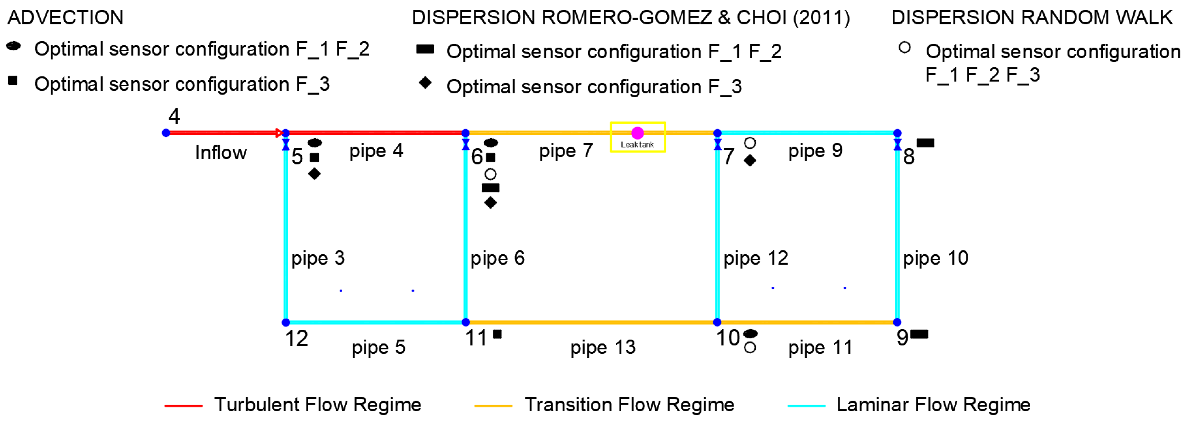
When the optimisation problem is solved using the three models previously analysed, very different optimum sensor configurations are obtained. Two possible configurations were obtained using the advective model for positioning the sensors, as presented in Figure 4.
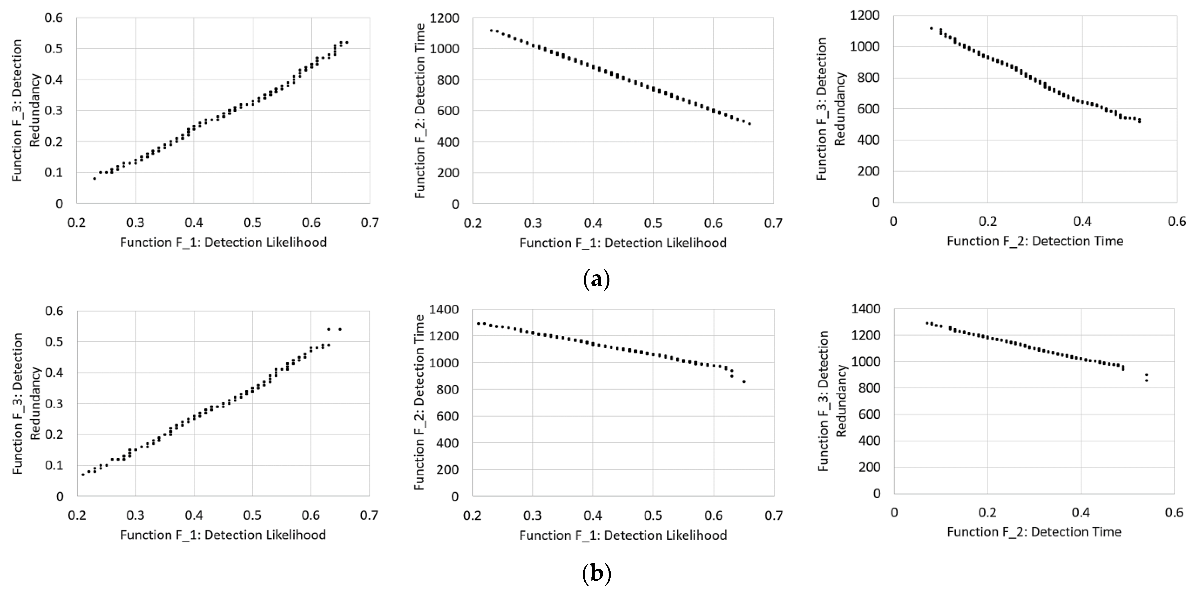
Table 1 shows the characteristics and performance of the optimal configurations for the three models. Solving the optimisation problem using the advective model made it possible to simultaneously optimise two objective functions (F_1 and F_2) using a single-sensor configuration (5–6–10). Node 11 must also be considered to maximise the objective function F_3. With three sensors in optimal positions, 66% of the contamination episodes were detected on average (maximum value of function F_1), and at least two sensors detected 52% within 20 min (maximum value of function F_3). The optimal average detection time was approximately 8 min. Figure 5a shows the obtained Pareto fronts for the three objective functions.
Using the AZRED formulations, the optimal solutions considering dispersion differ from the advective case by considering both the optimal sensor location and the objective function values (Table 1). As in the previous case, the objective functions F_1 and F_2 were maximised by the exact configuration of sensors (6–8–9), with values slightly lower than the previous values. As a result, the contamination event had a detection likelihood of 65%, and the optimal value of the detection time was somewhat more than 14 min. For the objective function F_3, the optimal redundancy value of 54% was obtained from a different configuration than the first method and included nodes 5–6–7. This is related to the importance of backward diffusive propagation, which is most evident in the laminar velocity profiles. Using the dispersive model, in which the dispersion was turbulent or transitional rather than laminar, the backwards diffusive propagation was less noticeable, as the dispersive behaviour was homogeneous across all network pipelines. Therefore, in this case, the discriminant that determines the redundancy phenomenon is a function of higher circulating water volumes (Figure 4). The Pareto fronts are presented in Figure 5b.
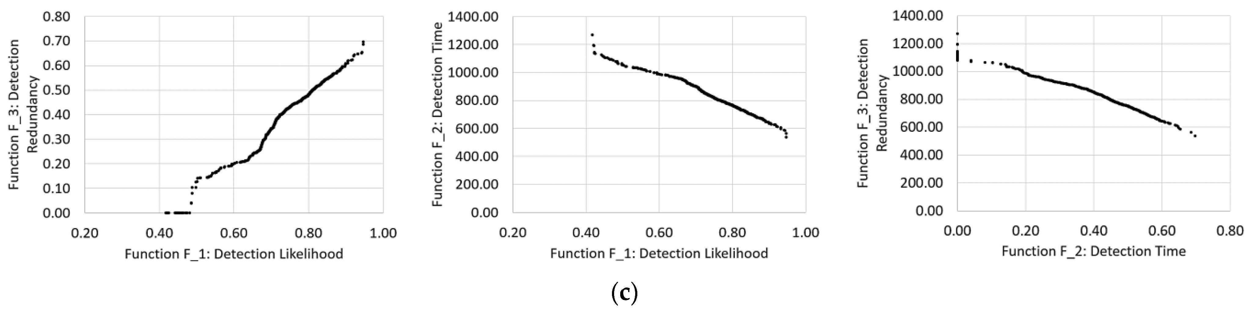
By solving the optimisation problem using the dynamic dispersive model (EPANET-DD), the three objective functions were optimised using a single configuration of three sensors positioned at nodes 6–7–10, which yielded better values than the other models (Table 1). In fact, with this configuration, 95% of the contamination episodes were detected on average, and at least two sensors detected 70% within 20 min. The optimal average detection time was approximately 9 min, slightly lower than what was obtained using the advective model. The Pareto fronts are presented in Figure 5c.
These three different optimal configurations for water quality sensor placement suggest the importance of correctly choosing the initial numerical model to be used for subsequent analyses. The use of a complete and accurate initial numerical model, which takes into account all the transport mechanisms that can occur within the water distribution networks, allows not only to reduce the number of sensors to be used for positioning (a single configuration to optimise all objective functions) but also to obtain the best parameter values for optimisation in terms of detection likelihood, detection time, and redundancy. This could be linked to the fact that diffusive—dispersive processes are intrinsically connected to the transport of pollutants within the water distribution systems. Furthermore, the different optimal configurations of the water quality sensors, obtained using the AZRED model and the EPANET-DD model, could derive from the different resolution hypotheses of the advection–diffusion–dispersion equations. Indeed, in the first case, the latter was solved using the Computational Fluid Dynamics Approach, performed using a finite volume-based solver, while, in the second case, the particle type model was solved using the random walk, which takes into account the randomness of the event.
4. Conclusions
This study solved the optimisation problem using the Monte Carlo method. It was applied to the laboratory network of UKE. Furthermore, three numerical models (EPANET, the AZRED model based on the formulations of Romero-Gomez and Choi, and a new model called EPANET-DD) have been considered to evaluate how they can influence the optimal positioning of water quality sensors in terms of the detection likelihood, detection time, and redundancy. In summary, the main conclusions of this study are summarized below:
- When the advective approach was used to solve the optimisation problem, the sensors were positioned in areas with high Reynolds numbers, where the flow regimes are predominantly turbulent and transition;
- The sensors were positioned in a linear pattern and covered most of the network using the dispersive AZRED approach;
- The EPANET-DD model provided the best performance, with a contamination event detection likelihood of 95%, a redundancy of 70%, and a detection time of approximately 9 min;
- Different configurations for sensor positions are obtained depending on the model used to solve the optimisation problem, as are different detection efficiencies for the objective functions. For example, the parameter values determined by the advective model are much lower than those determined by the dynamic dispersive model (EPANET-DD).
Author Contributions
G.F. designed the research; G.F. wrote the code; S.P., M.S. and G.F. performed the research; S.P. analysed the data; S.P., M.S. and G.F. wrote the paper. All authors have read and agreed to the published version of the manuscript.
Funding
This research received no external funding other than internal university funds aimed at technological advancement.
Data Availability Statement
Not applicable.
Conflicts of Interest
The authors declare no conflict of interest.
References
- Singh, R.B.; Kumar, D. Water scarcity. In Handbook of Engineering Hydrology: Environmental Hydrology and Water Management; CRC Press: Boca Raton, FL, USA, 2014; pp. 519–544. [Google Scholar]
- Aisopou, A.; Stoianov, I.; Graham, N.J.D. In-pipe water quality monitoring in water supply systems under steady and unsteady state flow conditions: A quantitative assessment. Water Res. 2012, 46, 235–246. [Google Scholar] [CrossRef] [PubMed]
- Li, T.; Winnel, M.; Lin, H.; Panther, J.; Liu, C.; O’Halloran, R.; Wang, K.; An, T.; Wong, P.K.; Zhang, S.; et al. A reliable sewage quality abnormal event monitoring system. Water Res. 2017, 121, 248–257. [Google Scholar] [CrossRef] [PubMed]
- Sambito, M.; Freni, G. Strategies for Improving Optimal Positioning of Quality Sensors in Urban Drainage Systems for Non-Conservative Contaminants. Water 2021, 13, 934. [Google Scholar] [CrossRef]
- Ostfeld, A.; Uber, J.G.; Salomons, E.; Berry, J.W.; Hart, W.E.; Phillips, C.A.; Watson, J.P.; Dorini, G.; Jonkergouw, P.; Kapelan, Z.; et al. The Battle of the Water Sensor Networks (BWSN): A Design Challenge for Engineers and Algorithms. J. Water Resour. Plan. Manag. 2008, 134, 556–568. [Google Scholar] [CrossRef] [Green Version]
- Preis, A.; Ostfeld, A. Multiobjective Contaminant Sensor Network Design for Water Distribution Systems. J. Water Resour. Plan. Manag. 2008, 134, 366–377. [Google Scholar] [CrossRef] [Green Version]
- Villez, K.; Vanrolleghem, P.A.; Corominas, L. Optimal flow sensor placement on wastewater treatment plants. Water Res. 2016, 101, 75–83. [Google Scholar] [CrossRef]
- Weickgenannt, M.; Kapelan, Z.; Blokker, M.; Savic, D.A. Optimal Sensor Placement for the Efficient Contaminat Detection in Water Distribution Systems. In Water Distribution Systems Analysis; ASCE: Reston, VA, USA, 2008. [Google Scholar]
- Murray, R.; Haxton, T.; Janke, R.; Hart, W.E.; Berry, J.; Phillips, C. Sensor Network Design for Drinking Water Contamination Warning Systems: A Compendium of Research Results and Case Studies Using TEVA-SPOT; EPA/600/R-09/141; Office of Research and Development, National Homeland Security Research Center: New Delhi, India, 2009.
- Perelman, L.; Ostfeld, A. Operation of remote mobile sensors for security of drinking water distribution systems. Water Res. 2013, 47, 4217–4226. [Google Scholar] [CrossRef]
- Oliker, N.; Ostfeld, A. Inclusion of Mobile Sensors in Water Distribution System Monitoring Operations. J. Water Resour. Plan. Manag. 2016, 142, 04015044. [Google Scholar] [CrossRef]
- Sankary, N.; Ostfeld, A. Inline Mobile Water Quality Sensors Deployed for Contamination Intrusion Localization. In Computing and Control for the Water Industry; Research Studies Press: Boston, MA, USA, 2017. [Google Scholar]
- Creaco, E.; Campisano, A.; Fontana, N.; Marini, G.; Page, P.R.; Walski, T. Real time control of water distribution networks: A state-of-the-art review. Water Res. 2019, 161, 517–530. [Google Scholar] [CrossRef]
- Isovitsch, S.L.; VanBriesen, J.M. Sensor Placement and Optimization Criteria Dependencies in a Water Distribution System. J. Water Resour. Plan. Manag. 2008, 134, 186–196. [Google Scholar] [CrossRef]
- Ohar, Z.; Lahav, O.; Ostfeld, A. Optimal sensor placement for detecting organophosphate intrusions into water distribution systems. Water Res. 2015, 73, 193–203. [Google Scholar] [CrossRef] [PubMed]
- Yang, X.; Boccelli, D.L. Dynamic Water-Quality Simulation for Contaminant Intrusion Events in Distribution Systems. J. Water Resour. Plan. Manag. 2016, 142, 04016038. [Google Scholar] [CrossRef]
- Abokifa, A.A.; Xing, L.; Sela, L. Investigating the Impacts of Water Conservation on Water Quality in Distribution Networks Using an Advection-Dispersion Transport Model. Water 2020, 12, 1033. [Google Scholar] [CrossRef] [Green Version]
- Taylor, G. Dispersion of soluble matter in solvent flowing slowly through a tube. Proc. R. Soc. London Ser. A 1953, 219, 186–203. [Google Scholar]
- Taylor, G.I. The dispersion of matter in turbulent flow through a pipe. Proc. R. Soc. London Ser. A 1954, 223, 446–468. [Google Scholar]
- Axworthy, D.H.; Karney, B. Modelling Low Velocity/High Dispersion Flow in Water Distribution Systems. J. Water Resour. Plan. Manag. 1996, 122, 218–221. [Google Scholar] [CrossRef]
- Romeo-Gomez, P.; Choi, C.Y. Axial Dispersion Coefficients in Laminar Flows of Water-Distribution Systems. J. Hydraul. Eng. 2011, 137, 1500–1508. [Google Scholar] [CrossRef]
- Piazza, S.; Blokker, E.J.M.; Freni, G.; Puleo, V.; Sambito, M. Impact of diffusion and dispersion of contaminants in water distribution networks modelling and monitoring. Water Supply 2020, 20, 46–58. [Google Scholar] [CrossRef]
- Rossman, L.A.; Clark, R.M.; Grayman, W.M. Modeling Chorine Residuals in Drinking-Water Distribution Systems. J. Environ. Eng. 1994, 120, 803–820. [Google Scholar] [CrossRef]
- Piazza, S.; Sambito, M.; Freni, G. A Novel EPANET Integration for the Diffusive–Dispersive Transport of Contaminants. Water 2022, 14, 2707. [Google Scholar] [CrossRef]
- Tarantola, A. Monte Carlo Methods. In Inverse Problem Theory and Methods for Model Parameter Estimation; SIAM: Philadelphia, PA, USA, 2004; pp. 41–55. [Google Scholar]
- Rossman, L.A.; Boulos, P.F.; Altman, T. Discrete volume-element method for network water quality models. J. Water Resour. Plan. Manag. 1993, 119, 505–517. [Google Scholar] [CrossRef] [Green Version]
- Lee, Y. Mass Dispersion in Intermittent Laminar Flow; University of Cincinnati: Cincinnati, OH, USA, 2004. [Google Scholar]
- Eliades, D.G.; Kyriakou, M.; Vrachimis, S.; Polycarpou, M.M. EPANET-MATLAB Toolkit: An Open-Source Software for Interfacing EPANET with MATLAB, The Netherlands. In Proceedings of the 14th International Conference on Computing and Control for the Water Industry (CCWI), Amsterdam, The Netherlands, 7–9 November 2016; pp. 1–8. [Google Scholar]
- Delay, F.; Ackerer, P.; Danquigny, C. Simulating Solute Transport in Porous or Fractured Formations Using Random Walk Particle Tracking: A Review. Vadose Zone J. 2005, 4, 360–379. [Google Scholar] [CrossRef]
- Kinzelbach, W.; Uffink, G. The random walk method and extensions in groundwater modelling. Transp. Process. Porous Media 1991, 761–787. [Google Scholar]
- LaBolle, E.M.; Fogg, G.E.; Tompson, A.F.B. Random-walk simulation of transport in heterogeneou porous media: Local mass-conservation problem and implementation methods. Water Resour. Res. 1996, 32, 583–593. [Google Scholar] [CrossRef]
Figure 1.
The layout of the experimental water distribution network.

Figure 2.
Overview of the experimental water distribution network (a), pumping system (b), and recirculation system (c).
Figure 2.
Overview of the experimental water distribution network (a), pumping system (b), and recirculation system (c).

Figure 3.
Installation of the pump-reservoir system (a) and connection to the node (b).

Figure 4.
Optimal sensor positioning for the UKE Laboratory Network.

Figure 5.
The Pareto front, including only advection (row (a)), dispersion (AZRED by Romero-Gomez and Choi 2011, row (b)), and dispersion (EPANET-DD) (row (c)): F_1–F_3 (left), F_1–F_2 (centre), and F_2–F_3 (right).
Figure 5.
The Pareto front, including only advection (row (a)), dispersion (AZRED by Romero-Gomez and Choi 2011, row (b)), and dispersion (EPANET-DD) (row (c)): F_1–F_3 (left), F_1–F_2 (centre), and F_2–F_3 (right).


Table 1.
Numerical analysis: Results of the Optimisation Problem.
| Advective Model | Romero-Gomez and Choi (2011) Model | EPANET-DD Model | ||||||||||
|---|---|---|---|---|---|---|---|---|---|---|---|---|
| Objective Functions | Optim. Values | Sensor Node Index | Optim. Values | Sensor Node Index | Optim. Values | Sensor Node Index | ||||||
| Detection Likelihood (F_1) | 0.66 | 5 | 6 | 10 | 0.65 | 6 | 8 | 9 | 0.95 | 6 | 7 | 10 |
| Detection Time [s] (F_2) | 517.13 | 5 | 6 | 10 | 858.54 | 6 | 8 | 9 | 538.96 | 6 | 7 | 10 |
| Redundancy (F_3) | 0.52 | 5 | 6 | 11 | 0.54 | 5 | 6 | 7 | 0.70 | 6 | 7 | 10 |
Disclaimer/Publisher’s Note: The statements, opinions and data contained in all publications are solely those of the individual author(s) and contributor(s) and not of MDPI and/or the editor(s). MDPI and/or the editor(s) disclaim responsibility for any injury to people or property resulting from any ideas, methods, instructions or products referred to in the content. |
© 2023 by the authors. Licensee MDPI, Basel, Switzerland. This article is an open access article distributed under the terms and conditions of the Creative Commons Attribution (CC BY) license (https://creativecommons.org/licenses/by/4.0/).
Share and Cite
MDPI and ACS Style
Piazza, S.; Sambito, M.; Freni, G. Analysis of Optimal Sensor Placement in Looped Water Distribution Networks Using Different Water Quality Models. Water 2023, 15, 559. https://doi.org/10.3390/w15030559
AMA Style
Piazza S, Sambito M, Freni G. Analysis of Optimal Sensor Placement in Looped Water Distribution Networks Using Different Water Quality Models. Water. 2023; 15(3):559. https://doi.org/10.3390/w15030559
Chicago/Turabian StylePiazza, Stefania, Mariacrocetta Sambito, and Gabriele Freni. 2023. "Analysis of Optimal Sensor Placement in Looped Water Distribution Networks Using Different Water Quality Models" Water 15, no. 3: 559. https://doi.org/10.3390/w15030559
Note that from the first issue of 2016, this journal uses article numbers instead of page numbers. See further details here.