Regionalization of IDF Curves by Interpolating the Intensity and Adjustment Parameters: Application to Boyacá, Colombia, South America

Abstract

Intensity, duration and frequency (IDF) curves are necessary tools for the design and construction of hydraulic projects. However, the pluviographic records needed to determine the IDF curves do not exist or are scarce. This research presents the regionalization of the IDF curves for the department of Boyacá, Colombia, which is made up of 16 municipalities including the provincial capital, Tunja. For the regionalization, the adjustment parameters (u and α) of the IDF curve stations in the study area were used. In the case of regionalization by the parameters found for the construction of the IDF curves, estimation methods with ordinary moments means and maximum likelihood were used. The regionalization and interpolation of the data were performed with Arcgis software. The resulting isoline maps were made in the case of regionalization intensities, and each map is associated with a different return period and duration to construct the IDF curves in the studied area. In the case of the regionalization maps, the parameters associated with each individual parameter were performed last. The results show that the use of IDF curve data is more accurate and reduces errors in the design. With the methods proposed in this study, IDF curves can be constructed for any site of interest that does not have rainfall stations.

1. Introduction

Intensity, duration and frequency (IDF) curves are necessary tools for the design and construction of hydraulic projects such as storm sewers, dams, reservoirs, water resources for power generation, flood control, drainage networks and the study of soil erosion [1]. With these curves, rain data return periods, including precipitation intensity and duration, are obtained for use in the hydraulic design of civil structures. Quantification of precipitation extremes is important in hydrologic designs to develop structural and nonstructural measures for flood protection, especially in urban areas. To evaluate the extreme character of rainfall in urban drainages, intensity–duration–frequency (IDF) relationships are used [2].

Because this information (IDF curves) is usually obtained in a timely manner for the site where the rain gauge or hydrometeorological station is located, it is of great importance to implement a practical methodology to determine the curves in places that do not have instrumentation. Pluviographic records are needed to determine IDF curves, which are the most suitable for this analysis. However, in many regions of the world, especially the third world, they do not exist or pluviographic data are only collected for a short duration [3]. Because of this, different alternatives will be discussed using two curve construction methods that allow regionalization.

The region of Boyacá (Colombia) was selected to conduct this project—in particular, the area bounded by the municipalities of Tunja, Pesca, Toca, Aquitania, Paipa, Combita and Cucaita. This geographical area was chosen due to the presence of pluviograph weather stations along with a significant amount of historical records of precipitation.

1.1. IDF Curves

IDF curves are plots resulting from the binding of specific points of the average intensity or depth intervals of varying lengths and in turn belong to the same frequency, which is also called a return period. The data are represented through a graphic on a Cartesian plane showing a series of graphical curves, one for each return period [4]. For the design of the hydrosystems, the use of IDF curves is a standard practice in many places because it incorporates the frequency and intensity of the maximum rainfall events of various durations [5]. The horizontal axis represents the duration, while the vertical one represents the intensities.

A typical procedure involves the following: (1) fitting a probability distribution to the annual maximum rainfall intensity values for several rainfall durations, (2) estimating extreme rainfall quantiles for each rainfall duration for a number of return periods, and (3) fitting a relationship between rainfall intensity and rainfall duration for each return period based on the rainfall intensity quantiles estimated for each rainfall duration. The resulting relationships between rainfall intensity and rainfall duration constitute the IDF curves for the given location [6].

IDF relationships of extreme precipitation are widely used for estimations during flood design. They describe the relationship between the mean precipitation intensity and frequency of occurrence (the inverse of the return period) for different time intervals of a given duration. These intervals, over which the precipitation intensity is averaged or ‘aggregated’, are called ‘aggregation levels’ or simply ‘durations. Conditioned on such durations, the conditional IDF relationships are essentially cumulative distribution functions of the precipitation intensity [7]. Because there is an interest in rather exceptional precipitation intensities (small frequency) during the design of storm water facilities, the distribution functions match extreme value distributions [8].

1.2. Regionalization of IDF Curves

As mentioned above, regionalization is based on the essential concept of hydrological homogeneity in a region, which implies the segmentation of the study area into regions with similar climatic and orographic characteristics (statistical homogeneity). Regionalization is often adopted in hydrology to help transfer information from gauged sites to others where information is not available. It is supported by investigation of the connections between hydrological responses and the elements affecting them and identifies regions with similar behavior. This transfer is generally based on a similarity measure, i.e., one tends to select catchments that are most similar to the site of interest. One widespread similarity measure is the spatial proximity [9]. An alternative similarity measure is the use of catchment attributes such as land use, soil type and topographical characteristics [10].

This concept is used for sites with a sufficient record length that consists of the quantile of the return period of extreme precipitation in a specific interest site; thus, a frequency analysis can be employed. However, some sites are not gauged at all and do not have long historical records available to make reliable predictions of extreme quantiles for larger return periods [11].

In regional rainfall frequency analysis, rainfall measurements from several sites in a specific area are combined for an estimation of the regional IDF curves. By utilizing regional data, the estimation uncertainty can be significantly reduced. Furthermore, by relating the extreme rainfall characteristics to relevant climatic and physiographic variables, IDF curves can be estimated at an arbitrary site in the region. Regional modeling includes three basic elements: the delineation of regions, an estimation of regional parameters, and determination of a regional distribution [12].

1.3. Application of Regionalization

The regionalization procedure provides products on demand for any user-selected location (gauged or ungauged) and does not cause discontinuities at boundaries that would result from delineation of distinct regions [13].

As mention above, the importance of using IDF curves when performing any work that is directly related to the hydrologic or hydraulic field is important. However, there are places or areas in which there is no specific information on a site of interest, usually because there is no instrumentation to measure parameters, such as precipitation, and weather measured as a daily event totalized (gauge) or registered as a real-time event, which implies the performance of hydraulic projects without this information.

Regionalization is a solution when there is a lack of information of this type because with triangulation, interpolation and extrapolation of data from pluviographic stations, an estimation of behavior in a given place can be obtained. Therefore, it is important to find alternatives that allow this regionalization to yield reliable data, such as the percentage difference compared with the same station, which is reliably compared to other methods.

Currently, for a hydraulic work, it is important to rely on information other than that from the nearest rain gauge station because there are many variables that generate sizable differences in the behaviors of distant places or when the distance is quite large [14]. Thus, regionalization aims to create an approach, without trying to be completely reliable, that provides a more accurate picture of the behavior of precipitation in an area (and running less risk than assuming misinformation from a different site to evaluate). It is worth noting that Boyacá Department (Colombia, South America) is a region of great importance in the Colombian economy and has experienced a drastic population increase in recent years. Furthermore, there are few studies related to this topic, and this implies that the information provided in this study will be of great value for the development of the region especially for agriculture and road infrastructure.

Among the foundations that underpin the design of hydraulic structures or systems and the design of an urban drainage is the knowledge of the precipitation events in the area. A specific storm is generally used, which is a critical and representative event in the region or a timely event that is planned to implement the design. Sometimes, an event that relates the interaction between rain intensity or depth, duration and frequencies or return periods subsequent to the site of execution or implementation of the project can also be taken.

Studies concerning regionalization of IDF curves in Colombia are scarce. There is one method that was endorsed by the National Roads Institute (INVIAS), where the country is characterized by areas or regions with similar behavior in terms of rainfall. In Colombia, information of IDF curves built from pluviographic stations is available from the Institute of Hydrology, Meteorology and Environmental Studies of Colombia (IDEAM) using a Gumbell method of construction and ordinary moments using probabilistic methods. Although these curves include historical precipitation information [15].

In this regard, we developed different methods, including the regionalization of the average characteristics of the basin, which are aimed to regionalize the maximum parameters to assess events for different return periods in places where there is no access to such information, for instance, pluviographic stations in this case and geomorphological or climatic support variables that are not easily measured or available.

2. Materials and Methods

The regionalization of the IDF curves relates three spatial parameters: the average intensity of precipitation, the event duration and the frequency of occurrence or return period. Therefore, in this case, it is necessary to look for alternatives to achieve the interrelationship of these three parameters in typical maps of regionalization.

The information shed by the IDF curves usually occurs with the duration on the horizontal axis and intensity on the vertical axis and shows a series of curves for each of the design return periods. These IDF curves result from joining the points representing the average intensity in intervals of different durations, and all correspond to the same frequency or return period. Together, with the definition of the curves, other elements to consider include precipitation intensity, frequency or probability of exceedance of a certain event. The IDF curves are able to show the mathematical relationship between rainfall intensity (i), duration (d), and return period (T) (the annual frequency of exceedance) [16].

The construction of IDF curves was completed using a univariate rainfall frequency analysis approach because of its mathematical simplicity [17]. The univariate approach for rainfall frequency analysis is explained in detail by Chow et al. (1988). In addition, most of the IDF curves were constructed using the window-based analysis approach where the durations are predetermined by time intervals.

This geographical demarcation zone is located in the department of Boyacá, Colombia. There are seven pluviographic stations with sufficient information (

Table 1. Intensity (mm/h) of the precipitation for two years at different stations.

Station	10 min	20 min	60 min	120 min	220 min	280 min	320 min
Uptc	31.99	26.19	14.70	7.82	4.67	2.95	2.13
Villa del Carmen	28.02	21.93	12.45	7.53	4.11	3.16	2.35
Tunguavita	64.16	47.92	24.00	14.41	9.11	7.33	6.56
Azulejos	26.91	19.52	9.99	5.95	2.88	2.08	2.35
Potrerito	20.42	15.48	8.96	6.31	4.11	2.79	2.51
Pesca	22.50	18.67	12.36	7.75	3.99	3.17	1.64
Tota	30.98	25.52	15.73	9.69	4.86	3.31	2.82

) and approximately 15–25 years of historical rainfall records. The year period covered by the data in all stations is between 1994 and 2019. Each weather station has different start years, but all have the same end year. The area of study is approximately 2622 km², and within this area, there are 23 towns or municipalities, including the capital of this department, Tunja. In the first instance, the information of the seven stations that compose the center zone of Boyacá was purchased. This analysis was implied from the passage of the graphic data into numerical data and the systematization of the data. For the IDF curves, each of the seven selected stations and the construction of these stations was performed using the probability distribution of type I (or Gumbell), and the parameters are obtained by the method of moments and maximum likelihood ordinary tests shown in Table 1. The meteorological stations are located within the department (state) of Boyacá, Colombia. The parameters or values $u$ and $\alpha$ are components of the fitting equations to a probability distribution.

An analysis was conducted of the different possibilities of interpolation that will produce IDF curves for the points not implemented within the study area. The map results were produced by the Software Support (ARCGIS). These maps show contour lines between selected stations of the studied area in the department of Boyacá. Two types of maps that can show U and parameters were developed to show isolines of the intensity of precipitation. With both parameters, IDF curves are built for any location within the area of study. The methods used for these analyses were based on calibration by modeling and extracting information from specific stations to develop a direct correlation and determine the variation and accuracy percentage. Moreover, a comparison between the results of this project with the data provided with the methodology currently used in Colombia and developed by the National Roads Institute (INVIAS) was performed.

Since the rainfall data represent a series of data that will be fitted to a probability function, it is necessary to perform a goodness-of-fit test. This test determines if the sample or data conform to the probability distribution that is being used, in this case, extreme value type I (EVI). This step is essential to determine if it is feasible to use a given distribution in a data series; In this case, for the sample of annual maximums, the Kolmogorov–Smirnov method was obtained, which allows calculating the relationship that exists between a distribution of a data sample and a theoretical distribution. The goodness-of-fit test requires that the test statistic value of the sample (Dn) be less than the tabulated value (Dn α) for the test to be accepted, the results for the stations shown in

Table 2. Kolmogorov–Smirnov test results.

Station	Dn. Máx.	Dn α
Tunguavita	0.14	0.2895
Potrerito	0.13	0.309
Villa Carmen	0.14	0.309
UPTC-Tunja	0.16	0.287
Tota	0.15	0.349
Pesca	0.14	0.361
Azulejos	0.18	0.301

[1,18].

Location

The project was developed in Colombia in the downtown area of Boyacá, where there are 16 population centers and some rural parts of other municipalities, as shown in Figure 1. Within these are the following municipalities: Motavita, Chíquiza, Sora, Cucaita, Oicatá, Chivatá, Toca, Siachoque, Pesca, Tota, Cómbita, Sotaquirá, Arcabuco, Samacá, Soracá, Firavitoba, Iza, Paipa, Tibasosa and Tunja (the department capital), among others. A search for stations with enough pluviographic information was conducted, and seven meteorological sites with 15–25 years of records were identified (

Table 3. Intensity (mm/h) of the precipitation for two years at different stations.

Pluviographic Station	Geographical Coordinates	Height above Sea Level
UPTC	Lat: 5.0°33.0′ N Long: 73.0°21.0′ W	2690 masl
Villa del Carmen	Lat: 5.0°30.0′ N Long: 73.0°29.0′ W	2600 masl
Tunguavita	Lat: 5.0°44.0′ N Long: 73.0°6.0′ W	2470 masl
Azulejos	Lat: 5.0°39.0′ N Long: 73.0°12.0′ W	2780 masl
Potrerito	Lat: 5.0°28.0′ N Long: 72.0°56.0′ W	3047 masl
Pesca	Lat: 5.0°31.0′ N Long: 73.0°4.0′ W	2678 masl
Tota	Lat: 5.0°34.0′ N Long: 72.0°59.0′ W	2900 masl

).

3. Results and Discussion

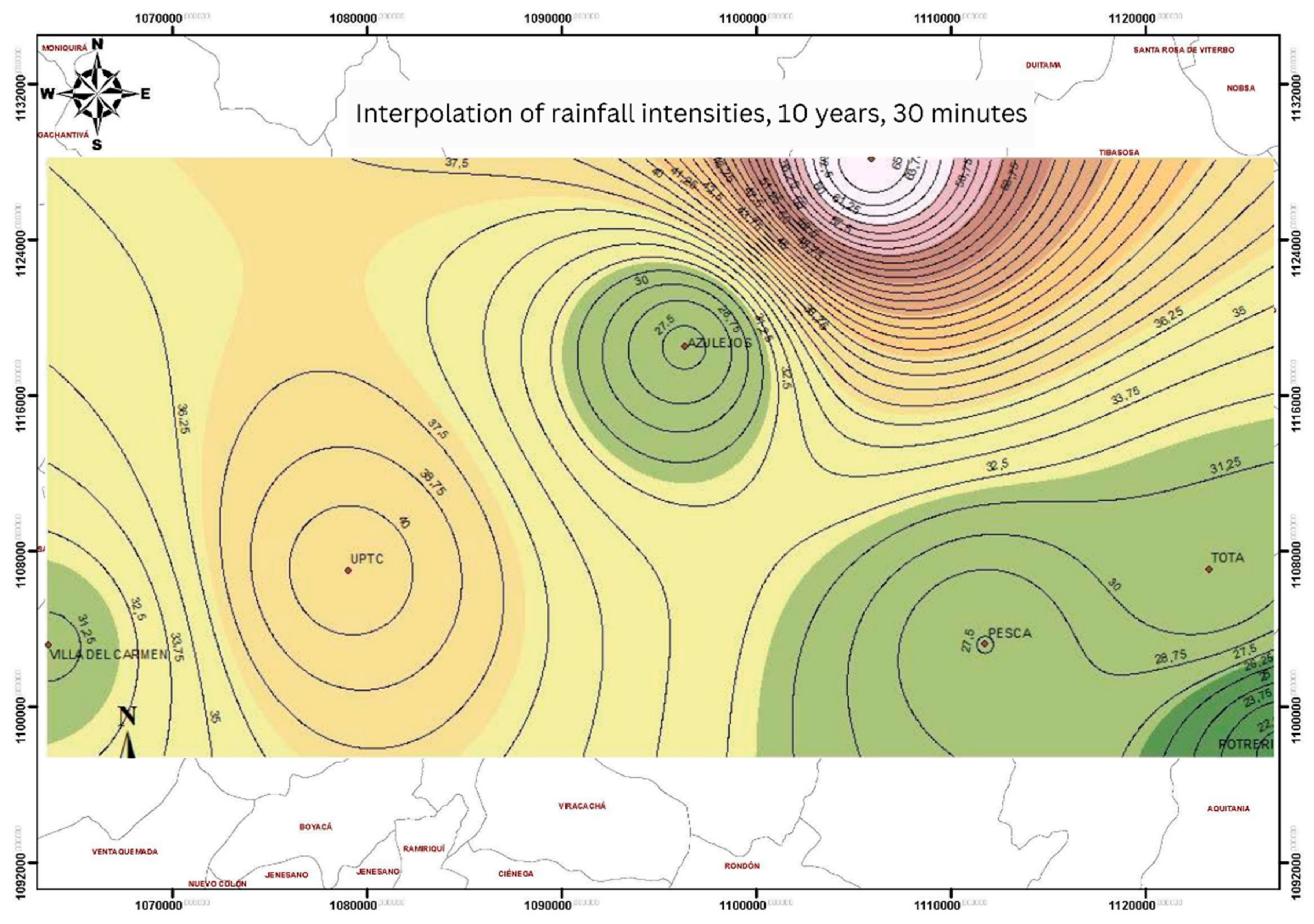
3.1. Regionalization by Intensity

In the interpolation by precipitation intensities, average rainfall intensity maps were generated corresponding to a return period and duration, that is, the reading of data to the intensity of the means associated with the fixed parameters; period of return and duration; therefore, to generate a curve, IDF, we have obtained the intensity of different maps, for example, for a curve with a return period of 2 years in this research, we have 9 maps, due to that the research was carried out with 9 durations (10, 20, 30, 60, 120, 180, 220, 280, and 320 min), that is to say that for the 8 return periods there are a total of 72 maps of isolines. In Figure 2, an example of the interpolation map of intensities is shown, where a return period and an intensity are related.

3.2. Regionalized $u$ and $\alpha$ Parameters

The information of the $u$ and $\alpha$ parameters that was referred to in the seven stations was obtained using the maximum likelihood method (EVI- ML). It is important to note that no methodology analysis of the ordinary moments (EVI -OM) was made to regionalize the parameters because the IDF results obtained are significant and the error is much larger when using this methodology compared with the EVI- ML method [1]. In

Table 4. $u$ and $\alpha$ parameters for all stations.

U Parameters
Duration (Minutes)
Station	10	20	30	60	120	180	220	280	320
	Intensity (mm/h)
Villa del Carmen	23.95	18.76	15.56	10.89	6.65	4.27	3.21	2.37	1.66
Tunguavita	54.38	41.63	34.20	20.85	12.45	9.01	7.72	6.06	5.35
Azulejos	22.80	16.57	13.24	8.66	5.22	3.28	2.19	1.49	1.79
Potrerito	16.64	12.87	10.56	7.99	5.83	4.43	3.63	2.21	1.92
Pesca	19.73	16.49	14.59	10.94	7.05	5.19	3.34	2.59	1.20
Tota	27.67	23.42	20.66	14.33	8.84	5.32	3.76	2.48	2.12
Uptc	13.85	11.15	9.56	5.18	2.29	1.43	1.15	1.42	1.28
$\alpha$ parameters
Villa del Carmen	11.11	8.64	6.91	4.27	2.38	2.57	2.46	2.16	1.88
Tunguavita	26.59	17.16	14.24	8.64	5.37	4.12	3.80	3.47	3.30
Azulejos	11.20	8.08	6.18	3.62	2.00	1.89	1.87	1.63	1.52
Potrerito	10.32	7.14	5.15	2.67	1.32	1.45	1.31	1.57	1.59
Pesca	7.54	5.95	4.56	2.57	1.59	0.77	2.31	1.66	2.01
Tota	9.08	5.72	4.68	3.83	2.29	3.23	3.01	2.26	1.91
Uptc	13.85	11.15	9.56	5.18	2.29	1.43	1.15	1.42	1.28

shows an example of the parameters for the $u$ and $\alpha$ values calculated by the EVI- ML.

Then, the parameters were organized in the seven stations. For the construction of IDF curves regionalizing by parameters, the generation of only nine isoline maps was required for the U parameter and only nine isoline maps for the $u$ and $\alpha$. Because this methodology does not depend on a specific period of return [14], the information was placed in Table 3.

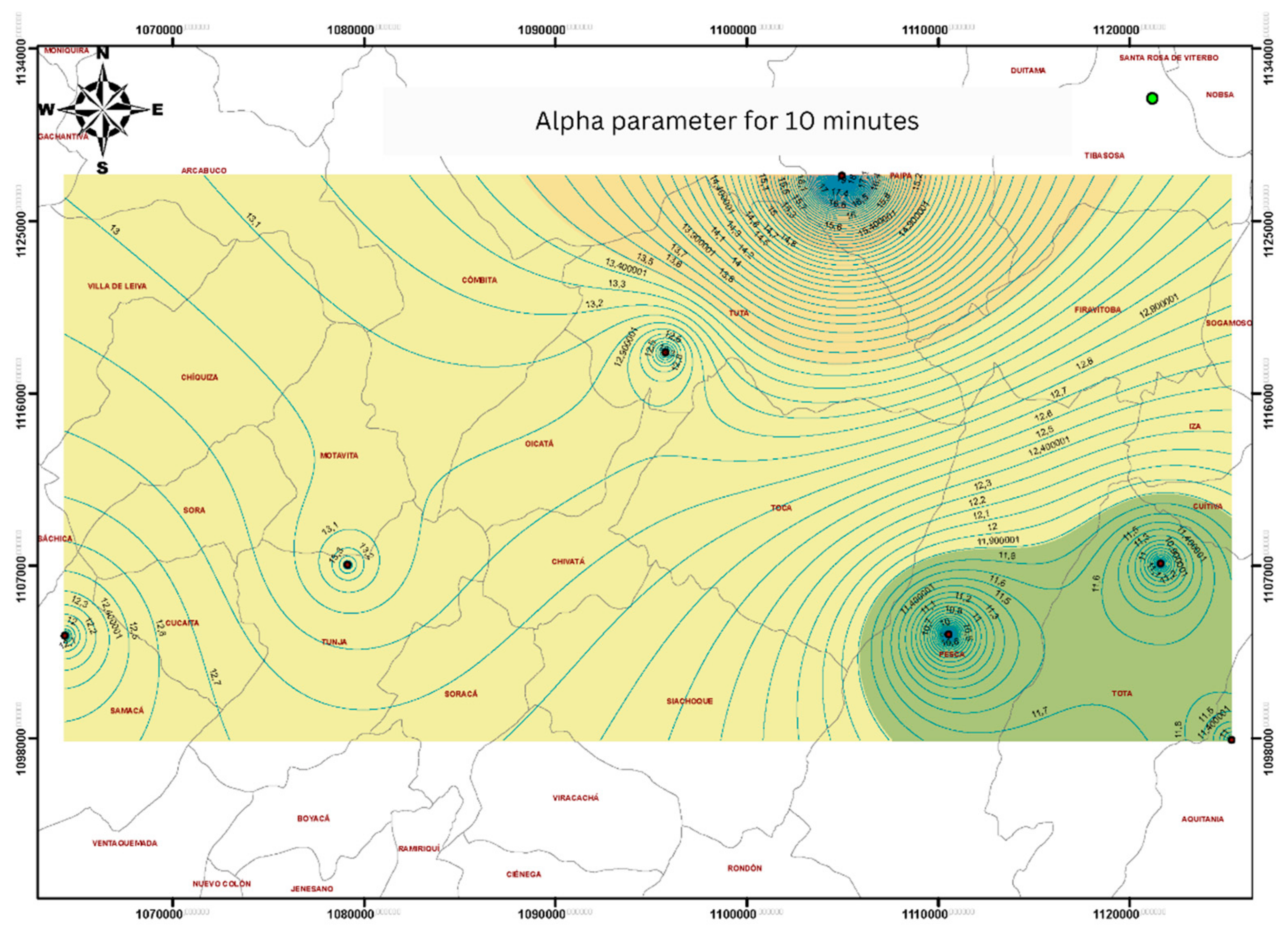
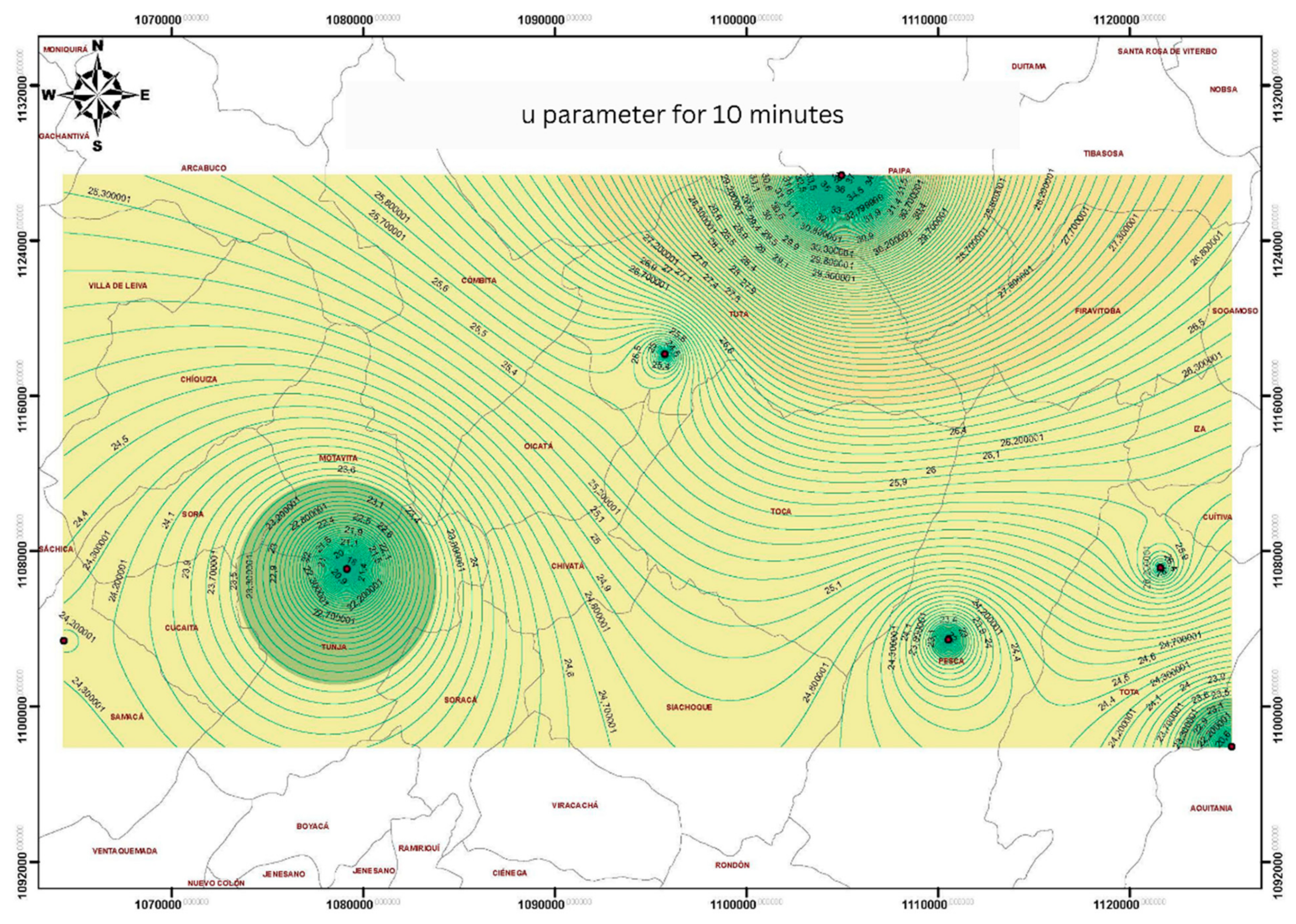
Subsequently, using the Ordinary Krigin method, each parameter received an interpolated value in relation to the duration and between seasons, which indicates that the $u$ and $\alpha$ parameter were interpolated, e.g., lasting 10 min. By interpolating, the curve iso-value maps of the $u$ and $\alpha$ parameters were obtained. This can be observed in Figure 3 and Figure 4 (how the isovalue curves represent each parameter).

3.3. Construction of IDF Curves by Regionalization

To construct the IDF curve, the $u$ and $\alpha$ values of each length were taken using the values of the parameters in the regionalized maps as shown in Figure 3 and Figure 4. After reading the $u$ and $\alpha$ parameters for each point of interest, the value only needs to be included in Equation (1), which is a function of the read parameters associated with the duration and the return period selected and where T is shown in Equation (2):

$$x_{\left(T\right)}=u+\alpha \ast y_T$$

(1)

$$y_T=-ln\left[ln\left(\frac{T}{T-1}\right)\right]$$

(2)

The intensity $x_{\left(T\right)}$ can be calculated by using the $u$ and $\alpha$ parameters as explained previously. $y_{T }$ can be calculated with T, which is the return period shown by the example in

Table 5. The $y_{T }$ value for each return period for Tunja station.

Return Period	${\mathit{y}}_{\mathit{T} }$
2	0.37
5	1.50
10	2.25
20	2.97
50	3.90
100	4.60
150	5.01
200	5.30

.

Thus, with the $y_{T }$ variable, the intensity can be calculated using equation1 mentioned above with the $u$ and $\alpha$ parameters previously obtained. Thus, a correlation can be obtained between each period of return and the intensity ($x_{\left(T\right)}$) as shown in

Table 6. Relationship between the return period (T) and intensity ($x_{\left(T\right)}$).

Period of Return (T) (Years)	Duration (min)
	10	20	30	60	120	180	220	280	320
	Precipitation Intensity (mm/h)
2	30.27	23.35	19.22	12.84	7.86	5.37	4.25	3.21	2.57
5	43.94	33.06	27.31	17.74	11.24	8.35	7.27	6.19	5.43
10	52.99	39.50	32.67	20.98	13.48	10.33	9.28	8.17	7.32
20	61.67	45.66	37.81	24.09	15.62	12.22	11.20	10.06	9.13
50	72.91	53.65	44.46	28.12	18.40	14.67	13.69	12.51	11.48
100	81.33	59.63	49.45	31.13	20.48	16.51	15.55	14.35	13.24
150	86.24	63.12	52.35	32.89	21.69	17.58	16.64	15.42	14.27
200	89.72	65.60	54.41	34.14	22.55	18.34	17.41	16.18	15.00

.

In the case of regionalization by intensities, each value should be read to obtain the information from the IDF curves for the site of interest. For that purpose, it should take 72 data points in total; regionalization counterpart parameters must be obtained by reading $u$ and $\alpha$ data from the 18 maps in total. The regionalization intensity data obtained by EVI-OM had higher error rates compared with EVI-ML because the method of the probability weighted moments (ML) performs a calculation parameter from the observed ordinary moments (OM). In general, the number of stations is acceptable due to the extension covering the study area, but it is important to note that if there were more stations or pluviographic information within the study area, triangulations and interpolations would be more accurate, which translates into a better description of the typical behaviors of specific areas where they seek to find the values of intensity. The central zone of the department of Boyacá, Colombia, presents a high degree of homogeneity, classified as region 1 or Andean region, due to its similarity of climatic and meteorological condition [19].

To implement the methodology of the ordinary moments EVI-OM and to vary the weighting factor (m), the error rate is increased so that these values are not considered in this research. By using regional data, it highlights that by using data from the IDF curves, the results are closer to the actual data and are more accurate compared to the simplified method. The reason is that in the simplified method, the waterworks are oversized, which generates errors in the designs due to the inefficiency and ineffectiveness; plus, there is greater construction time and more significant cost overruns (poor planning for headworks).

The proposed methodology for regionalization of the IDF curves is practical and infers a more scientific process in obtaining this hydrological parameter in places with little information or with outdated methods for obtaining these curves. When comparing IDF curves from common methods with the method proposed in this research, a difference of 0.11% was found for periods of low return, and it increased to 52% for periods of high return (200 years), which shows the importance of the present research for future investigations. In

Table 7. Comparison between the method propose in this investigation and the normal or common method and the propose by the INVIAS.

IDF INVIAS vs. IDF Common Method.
Period of Return (T) (Years)	Duration (min)
	10	20	30	60	120	180	220	280	320
	Precipitation Intensity (mm/h)
2	86%	44%	27%	24%	47%	54%	66%	123%	183%
5	47%	14%	1%	4%	30%	42%	53%	71%	99%
10	37%	7%	−6%	0%	27%	41%	51%	57%	78%
20	32%	3%	−8%	−2%	26%	42%	53%	51%	68%
50	31%	2%	−9%	−1%	29%	47%	58%	48%	63%
100	33%	4%	−8%	1%	33%	52%	64%	49%	63%
150	34%	5%	−7%	2%	36%	56%	68%	51%	64%
200	36%	6%	−6%	4%	38%	59%	71%	53%	65%
IDF interpolated by parameters vs. IDF common method.
2	−5%	−11%	−15%	−13%	1%	−6%	−9%	9%	21%
5	−8%	−15%	−19%	−14%	8%	14%	22%	36%	52%
10	−9%	−16%	−20%	−14%	11%	23%	36%	46%	62%
20	−9%	−17%	−21%	−15%	13%	30%	46%	52%	68%
50	−10%	−18%	−21%	−15%	15%	37%	57%	58%	73%
100	−10%	−19%	−22%	−15%	17%	41%	63%	61%	76%
150	−10%	−19%	−22%	−15%	17%	43%	66%	62%	78%
200	−11%	−19%	−22%	−15%	18%	44%	68%	63%	79%
IDF interpolated by intensity vs. IDF common method.
2	−5%	−11%	−15%	−12%	1%	−5%	−8%	11%	27%
5	−7%	−14%	−19%	−13%	2%	11%	15%	23%	34%
10	−8%	−15%	−20%	−13%	3%	19%	27%	28%	37%
20	−9%	−16%	−21%	−14%	5%	24%	35%	31%	38%
50	−10%	−17%	−21%	−14%	5%	30%	43%	33%	39%
100	−10%	−17%	−22%	−14%	6%	34%	48%	35%	40%
150	−10%	−17%	−22%	−14%	6%	36%	50%	35%	40%
200	−10%	−18%	−22%	−14%	7%	38%	62%	36%	41%

, shows the results of comparison between the method propose in this investigation and the normal or common method and the propose by the INVIAS.

The present work showed how this method is a viable alternative to the currently used methods in Colombia, where presently, differences of more than 183% or more, can be found between IDF curves of a specific station compared to a regionalized IDF curve. The proposed method can be extended and improved by involving variables that were not considered such as the height above sea level, the specific weather, and the generation of geographical divisions or sub-regions based on the similar behavior of historical precipitation.

It is important to highlight that the main and remarkable result is that a new method is proposed to determine the IDF curves in places where there is no information or climatological measurement, approximate and reliable to the few existing ones. However, it is necessary to propose new research’s where the accuracy of the method is deepened, using other types of interpolation and especially in more instrumented countries.

4. Conclusions

The method of estimating IDF curves by means of interpolation of adjustment parameters u and α presents better management or ease of calculation, due to the need for a lower reading of data in the maps, but it is contrasted against the accuracy, because it shows greater differences compared to the real values, even compared to the synthetic method.

Analyzing the resulting information in the cross-validation of the IDF curve interpolation methods, it was clearly shown that the method of interpolation of mean precipitation intensities and interpolation of parameters presents similar values to the real values. There wee no marked behavior trends.

In the comparison of the interpolation methods proposed in this research to the real values, a similar behavior was observed; but in all cases, the method of interpolation by intensities presented the smallest difference, and therefore a closer proximity to the real data, for such a motif is the method that is recommended to be used in similar processes, both research and application.

The largest differences compared to the actual values are presented in both methods in durations over 120 min, independent of the return period, which suggests that the methods must be used carefully analyzing the design requirements. On the other hand, the method of interpolation by average intensity presents a minor difference compared to the real values in durations equal to 120 min and low return periods. For this reason, it is advisable to use this method for rainfall runoff models approaching the duration mentioned.

A concentration of data was presented towards certain meteorological stations in interpolating precipitation intensities. This result can be easily seen on maps and this pattern is called a “bull’s eyes”. This is another reason to discard the interpolation of precipitation intensities as a method that allows regionalizing the IDF curves in a precise way.

The construction of IDF curves by the method of interpolating parameters represents a possibility to more precisely determine the IDF curves in places that do not have meteorological instrumentation. This method must be tested in other areas to verify the different limitations or advantages.

The method of interpolation of mean intensities of precipitation for the estimation of IDF curves proposed in this research, in comparison to the method of estimation of curves IDF proposed by the INVIAS, has a better behavior since it better approaches the actual data, presenting smaller differences. It should be noted that the methods are only comparable from the standpoint of results, because the interpolation methods are based on pluviographic records unlike the study by Vargas M and Diaz-Granados, which is based on pluviometric records.

The type of interpolation that is used has to be investigated in greater depth if the proposed method is applied, since it presents a concentration towards the measured points. In similar cases, subjective interpolation methods can be used in order to minimize the error. It is advisable to extend the research to interpolation methods such as IDW, Spline and the different types of Kriging, assessing height changes and different types of climatic behavior.