
A Detailed Analysis on Hydrodynamic Response of a Highly Stratified Lake to Spatio-Temporally Varying Wind Field

1
Department of Civil and Environmental Engineering, Tokyo Metropolitan University, Tokyo 192-0397, Japan
2
Department of Civil Engineering, Kobe University, Kobe 657-8501, Japan
*
Author to whom correspondence should be addressed.
Water 2023, 15(3), 565; https://doi.org/10.3390/w15030565
Submission received: 28 November 2022
/
Revised: 23 January 2023
/
Accepted: 25 January 2023
/
Published: 1 February 2023
(This article belongs to the Special Issue Urban Water-Related Problems)
Abstract
:Wind is generally considered an important factor driving the transport and mixing processes in stratified enclosed systems such as lakes and reservoirs. Lake Abashiri is one of the instances of such a system. For these systems, typically, the temporally unsteady but spatially uniform nature of wind has been assumed for simplicity. However, the spatial non-uniformity of wind could significantly alter compound hydrodynamic responses. In this study, such responses were investigated under the continuous imposition of different inhomogeneous wind conditions by applying numerical models and integrated analysis. The resultant tracer transport in both uniform and non-uniform wind cases was insignificant for the total study period of 9 days. However, under the short interval of , where is the internal fundamental period, different behaviors of both surface particle transport and the internal wave field were identified. Particularly, surface mass transport responses to higher spatial wind variance were obviously different from those in the uniform case. In addition, internal wave spectra under strong wind magnitude, which has low spatial variances, became identical to that of uniform wind; however, there were some discrepancies in the non-uniform case in the wave spectra under the influence of weak-to-moderate wind of high spatial variances. The results could provide an in-depth understanding of the lake’s hydrodynamic response to inhomogeneous wind which could improve water management in lakes and reservoirs.
1. Introduction
Water quality in lakes and reservoirs has implications for its beneficial applications, such as fisheries’ management, water supply quality, phytoplankton population, and control of the manganese level [1,2,3]. Such conditions are controlled by both nutrient loadings and physical factors such as mixing, and transport processes driven by winds [4]. As a major source of energy in lakes, coastal waters, and some estuaries, wind forcing plays an important role in the formulation of lake mixing, circulation, and internal seiche excitation [5,6,7]. Wind blowing over a lake rapidly distributes its momentum to water and consequently induces surface current and transport of floating objects such as phytoplankton along the wind direction. In addition, turbulent mixing induced by wind can affect the structure of the stratification, leading to changes in hydrodynamics and, in turn, species composition, proliferation of toxic algae, and dwindling of drinking water supplies [8,9].
Information on wind-induced transport, mixing, and internal waves is typically explained by numerical approaches, whereby the source of wind input is frequently retrieved from a point-based stationary wind field to spatially represent the phenomenon [5,7,10,11]. However, such an assumption is often oversimplified, although its dependency on the surrounding orography is crucial, resulting in a lack of spatial representation of the inhomogeneity of actual meteorological conditions [12]. Moreover, spatial wind fields often vary across large lakes due to pressure gradients over the water surface [13], and across small lakes due to sheltering effects [14,15]. Consequently, wind-induced lake hydrodynamics are insufficiently explained with the inaccurate surface boundary condition. Therefore, the coupling effects of the horizontally non-uniform wind and the real bathymetry of the concerned study sites are needed to realistically simulate the phenomena [16,17]. This could be achieved through a stand-alone uncoupled hydrodynamic model interacting with spatially interpolated wind [18,19], climate products [20], and numerical downscaling methods [12,21].
Generating the spatial variability of wind either by observation or by numerical simulation illustrated improvements in hydrodynamic simulations that were underpinned in a number of studies. For example, the simulation in Lake Kinneret in Israel improved the wave amplitudes and reduced the overall phase error after the spatially inhomogeneous wind stress was appropriately estimated [22]. The flow structure in Lake Belau changed drastically under the induction of spatial variation in the wind [23]. In Lake Ledro, TKE and its dissipation rate were reduced because of the representation of spatially inhomogeneous wind, as they are sensitive to the wind intensity [14]. The assumption of wind uniformity may often fail to reproduce the natural circulation condition and its characteristics in Spermberg Reservoir [24]. The spatial variations in the wind field separated the natural internal seiche excitation into different modes, as well as acting as a controller for higher horizontal modes in Lake Iseo [15]. Furthermore, the spatial variations in wind-generated wind curl, formulating seasonal regimes of Ekman layers resulting from the accumulation of particulate organic matter (POM) at the Tokyo Bay head, are driven by the pumping velocity [25]. Normally, comparisons of the response of lake hydrodynamics to spatial uniform and non-uniform wind fields are done with visualization, without being quantified. Quantification of these phenomena based on wind inhomogeneity levels is therefore necessary to elucidate their in-depth features.
To understand the complicated response of hydrodynamics to spatial and temporal variations in wind, meteorological wind-induced lake hydrodynamics were numerically simulated in Lake Abashiri from 21 November to 29 November 2011. To the best of our knowledge, this study is the first to quantify the interactions between spatial variations in wind forcing and lake hydrodynamics in Lake Abashiri. Therefore, under different spatial and temporal wind conditions, there are three main objectives in this study: (1) to quantify and understand the effects of wind forcing on surface mass transport and water current; (2) to quantify the effects of wind forcing on tracer movement; and (3) to estimate the potential mixing and to quantify the effects of wind forcing on internal seiches. The overall aim is to elucidate and quantify the differences in lake hydrodynamics between spatially uniform and spatially non-uniform wind.
2. Materials and Methods
2.1. Site Background
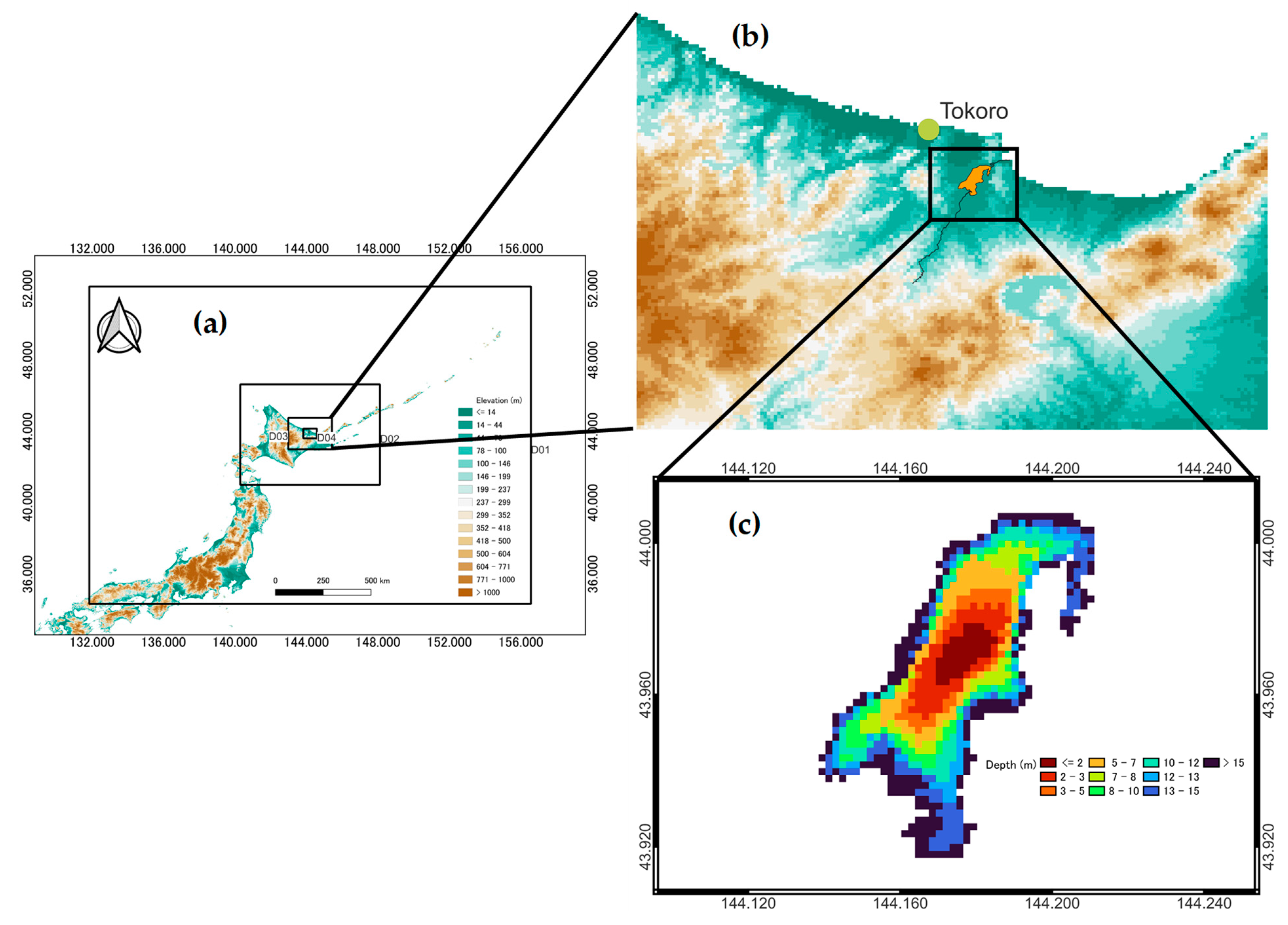
Lake Abashiri in Hokkaido (Figure 1a) is a small lake with a surface area of 32.87 km2, a shoreline of 42 km, a maximum depth of 16.1 m, a mean depth of 7.2 m, and an altitude of 0.4 m. Lake Abashiri connects Abashiri River at the southernmost part of the catchment area and estuary at the northeast end (Figure 1b). Seawater frequently flows backward from the sea to the Abashiri River, so that the lake is stratified mainly with salinity. Lake Abashiri is an example of a highly stratified system linked by upstream freshwater intrusion and downstream seawater intrusion. This complex system forms a strong halocline, distinguishing the lake’s layers. The lower layer of saline water is deoxidized up to <0.1%Sat due to a long residence time [26]. The lake provides important recreational activities, such as fishing and sports, throughout the season. However, eutrophication has recently become a concern due to the nutrient loading [27]. Lake Abashiri can emit 11% of the total methane in Lake Hokkaido and produce dissolved methane (DM) concentrations five times higher than the estimated one-dimensional methane model (DM concentrations were estimated by surface area) [27]. Such an issue could be problematic if the lower-layer gas was released from the lake. As an important factor of such a system, continuous wind exceeding 10 m/s could upwell the lake, releasing CH4 to the environment [7].
2.2. Observation Data
Hourly values of wind speed and direction taken from Tokoro station (Figure 1b) from 21 November 2007, to 30 November 2007 were obtained from the Automated Meteorological Data Acquisition System (AMeDAS) which was then used to validate the WRF model. AMeDAS is a collection of Automatic Weather Stations (AWS) and is monitored by the Japan Meteorological Agency (JMA) [28].
2.3. Weather Research and Forecasting Model (WRF)
This study employed WRF for numerically downscaling and simulating wind inhomogeneities [29] with four nested domains (Figure 1a), with 200 × 200, 190 × 190, 178 × 178, and 166 × 166 cells and horizontal resolutions of 10 km, 3.3 km, 1.1 km, and 333 m, respectively. The temporal resolution was set for every 20 min. Table 1 illustrates WRF configurations and the domain setup for the simulation. In the resolution from the outermost to the innermost domain, the former covers almost the entire country of Japan to capture overall atmospheric phenomena, while the latter includes Lake Abashiri surrounded by a relatively flat area. In this context, hourly ERA5 [30] reanalysis data were dynamically downscaled from 0.25° spatial resolution. ERA5 is the most recent global reanalysis product that has benefited from a decade of advancing model forecasting and assimilation methods [31]. In addition, studies have reported that ERA5 is good at improving simulation in complex terrains and outperforms several other global reanalysis products in terms of surface wind [32,33,34]. We used the rapid radiative transfer model (RRTM) scheme for longwave radiation and the Dudhia scheme for shortwave radiation. Furthermore, we applied the Monin–Obukhov scheme [35], the Noah-MP land-surface model, and the Mellor–Yamada–Janjic TKE scheme for the surface layer, land surface, and planetary boundary layer, respectively. In addition, substitution of higher land-use resolution taken from Global Map Japan [36] and observation-based dynamical nudging to the initial conditions were implemented to further improve model performance. Each run began at 00:00 UTC and generated outputs every 20 min.
2.4. Fantom-Refined Hydrodynamic Model
The Fantom-Refined [37,38] model was developed following equations of continuity and 3-D Navier–Stokes with incompressible and Boussinesq approximation together with thermal flux (details of the model can be found in Appendix A). The model is further improved with a local mesh refinement (LMR) technique based on a structured grid which uses rectangular grids similar to a tree-based grid. This method uses two different perspectives of a horizontal grid, macro, and micro views. The macro view determines the refining unit (hereafter the “container”), and each container is discretized in a structured manner with arbitrary horizontal resolution (hereafter the “micro view”). This method introduced the concept of a container that defines local groups with constant grid resolution in each direction. With this container, we may specify any computational cell in the domain with a simple, modifiable LMR and straightforward indexing. The study, however, applied only the macro view for simplification and for computational efficiency.
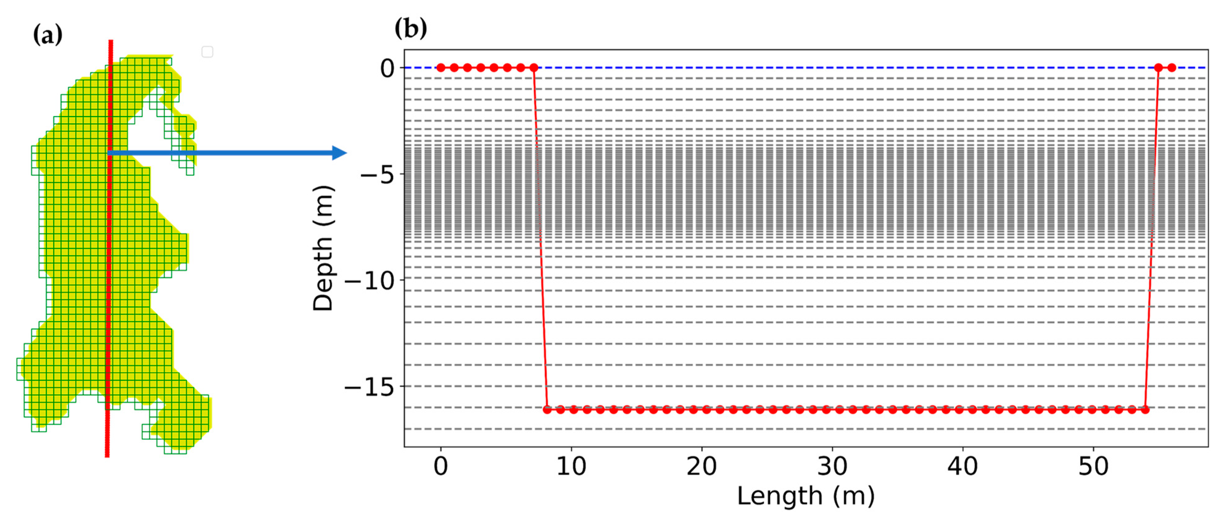
The horizontal resolution for the hydrodynamic model was set at 200 m in each direction (Figure 2a). In terms of vertical resolution, finer grids (0.1 m) were set at the middle of the lake’s depth to represent the halocline fluctuations visibly and accurately, while coarser grids were used at the remaining depths (Figure 2b). Vertical temperatures were distributed evenly along the depth, and salinity was initialized with measured data, in which the halocline existed at a depth of approximately 5 m below the water surface.
Complexity exists when a clear understanding of lake hydrodynamics is challenged by both spatially varying drivers (wind and bathymetry), whereby lake hydrodynamics potentially react differently under the spatial distribution of the former, which is controlled by the surrounding orography. Meanwhile, variations in depth and geometry of the latter are of great concern in further alternating the mechanism. A deep comprehension of how a specific main driver affects hydrodynamics is the key to gaining a step-by-step understanding of the complex physical behavior of lake hydrodynamics. Therefore, flat bathymetry of 16 m was assumed to separate the complex effects of the real bathymetry.
To investigate the effect of spatial and temporal variations in wind on hydrodynamics in the lake, a comparative study was conducted between unsteady but spatially uniform wind, and unsteady and spatially non-uniform wind (Table 2). By a simple interpolation technique, the horizontal and temporal resolutions of the wind field extracted from the fourth domain of the WRF model were refined to 200 m and 10 s, respectively, to match those of the hydrodynamic model. The uniform wind field was created by taking wind data at the center grid of the lake. Wind shear stress applied over the water surface was computed explicitly with the function of (U10) [38].
where is the air density, is the drag coefficient, and is the wind magnitude at 10 m above the water surface, i.e., U10. The model applied a bulk formula [39] to estimate sensible and latent heat fluxes, and short and long wave radiations from meteorological weather conditions.
2.5. Indicators for Spatial Variations in Wind Heterogeneity
Quantification of wind inhomogeneities is challenging due to the complex distinction between wind direction and wind speed. Recently, several studies have attempted to quantify the spatial variations in wind. For example, smaller root mean squared errors of vectors u and v indicated uniformly spatial variations and vice versa [14]. This technique, however, using the vectors u and v, cannot quantify the invariance of wind speed or wind direction, which could be directly addressed using 2D mean filter analysis [40].
The spatial consistency of the wind was determined based on the integrated coefficient of variance and a 2D mean filter [40].
where is the filtered image, is an integer and can be selective with incremental size (e.g., 1, 2, 3, …, m), m is arbitrarily chosen for grid size, is the value in each pixel of the grid of the previous filtered image; and s and z are the corresponding coordinates of the grid itself. As noise reduction comes at the expense of blurring the image (a 2D visual representation of any pixel), if the resulting image () has features in common with all the previous filtered image (), the wind field will be considered to be spatially homogeneous. Details of the computation procedures are described in Appendix B.
2.6. Indicators for Temporal Variations in Wind Heterogeneity
The metric Pearson correlation was applied to measure the linear relationship between two sets of data. It is the ratio of two variables’ covariance to the sum of their standard deviations.
where overbar and are the average value of the sample population, and is the sample size. To analyze the homogeneity of temporal wind field, a correlation map constructed between the center grid (the 2D time series data at the center of the chosen dataset) and the surrounding ones was calculated during the simulation period.
2.7. Wedderburn Number
The Wedderburn number, a non-dimensional and systematic relationship between the wind-induced shear stress and the baroclinic pressure gradient, was computed to identify the mixing condition in the reservoirs and lakes [41].
in which is the epilimnion depth, is the wind fetch length, is the friction of wind velocity, and is the reduced gravity.
2.8. Surface Particle Transport, Tracer Simulation, and Internal Seiche
In principle, wind triggers two main important physical phenomena, lake circulation and surface and internal waves, both of which control the mass transport in lakes. To investigate the movement of the former, virtual particles are often placed and numerically simulated together with the atmospheric forcing interaction. This approach can be visually quantified by the Lagrangian tracking method, whereby the simulated particles often representing phytoplankton, fish eggs or larvae, are released, and the dynamics of the particle trajectories are recorded in time and space over the lake [12,19,21]. In this study, surface particles were placed uniformly on the water body to elucidate the effect of spatial and temporal variations of the wind field. In addition to the Lagrangian tracking method, tracer tracking is frequently adopted for its representation of either two- or three-dimensional transport of fluid containing pollutant [10,20]. To this aim, a normalized tracer concentration of 1.0 was set at the northern part of the lake.
Investigation on the development of the two-layer model of the temperature profile [42] was the key to further intensive empirical studies in an effort to classify the mixed-layer dynamics in lakes [43] and to readily determine the first vertical internal wave mode V1H1 [44]. To get a better insight into the internal waves that are generated by both homogeneous and inhomogeneous wind, a temporal variation of density interface for each simulation period was extracted. After that, spectral analysis was applied to evaluate and highlight the periodic evolution of internal seiches in both uniform and non-uniform cases. This technique can easily reveal hidden oscillatory motions in a time series structure or can detect the dominant frequencies of a periodic time series in terms of both spatial and temporal resolution [45]. Welch’s method was used to estimate power spectral density (PSD), where the Hanning window function was adopted to weight the time series dataset.
Standing internal waves in confined basins can be categorized by nodal points on the vertical (V) and horizontal (H) components, VaHb, where and are the fundamental vertical and horizontal mode components, respectively [46]. Finally, we computed analytical internal waves based on the calculation described in [6] to theoretically identify the period of each mode. We also compared the performance of the numerical model forced by different simulation periods with the analytical model in a variety of wind conditions. Based on the procedure described in [6], the periods of internal seiches were estimated by a 1D multi-layer hydrostatic linear model as
where and are the fundamental vertical and horizontal modes, respectively, is the gravitational acceleration, and is the eigenvalues assuming a two-layer model system ( = 1). The fundamental period can also be calculated following the Merian formula:
where is the reduced gravity of the two-layer system, and are the densities of the two layers, respectively, is the thickness of the upper and is the thickness of the lower layer. Additionally, the fundamental period can also be estimated as .
3. Results
3.1. WRF Model Validation
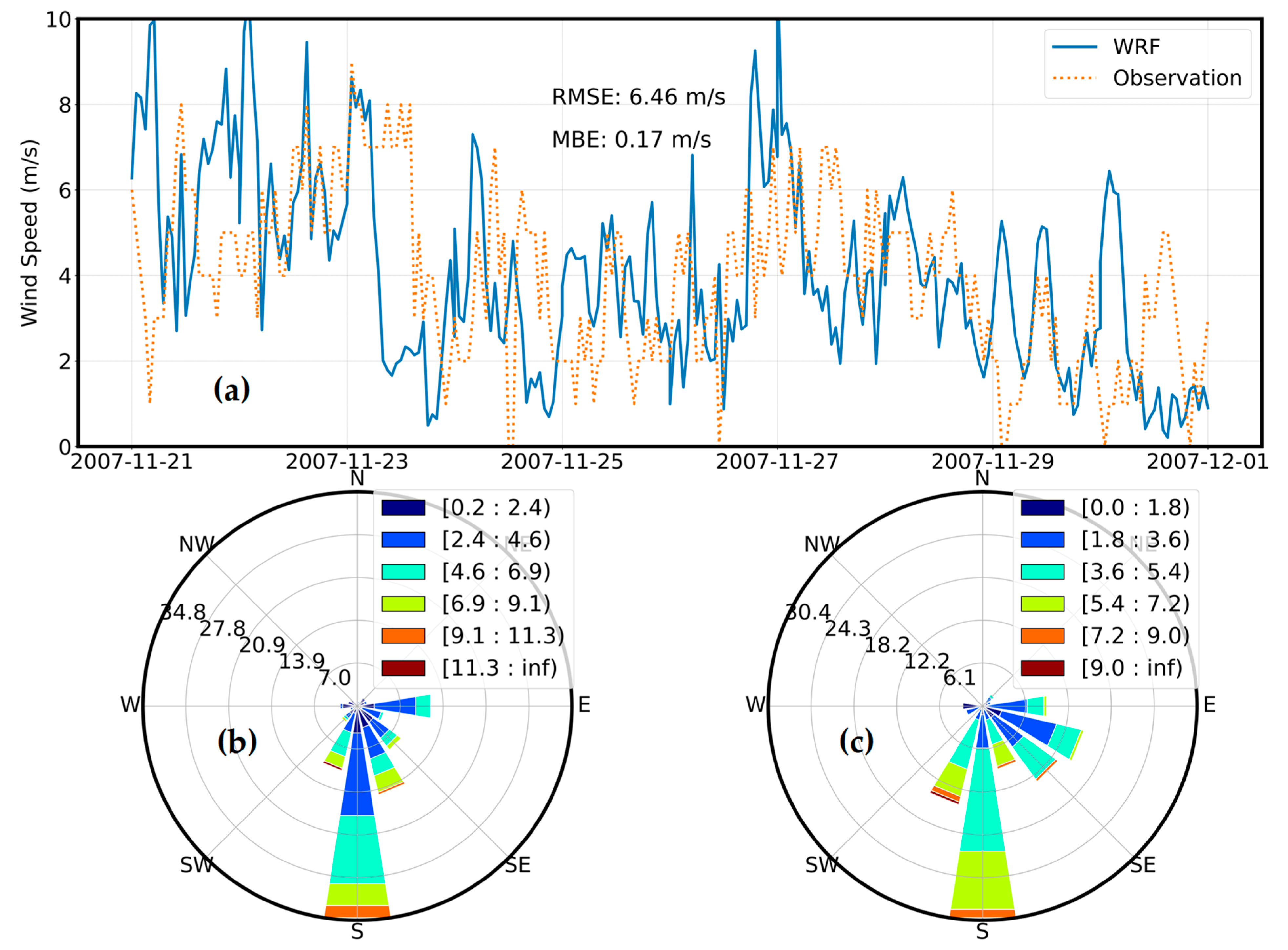
Wind data taken from AMeDAS (Figure 3a) illustrated a strong north-easterly wind with a clear diurnal-cyclical alteration during the simulation period. Strong winds evolved during the early morning and weakened from the beginning of the afternoon until nocturnality, with a high frequency of maximum and minimum intensities of approximately 10 m/s and around 2 m/s, respectively. These periods with strong magnitudes and clear periodicity could potentially influence the synoptic-scale occurrences related to the lake’s hydrodynamics. From the 24th to the 26th, low to moderate magnitudes were noted, with a tendency toward mild fluctuations. Validation between the model and observed data showed the general overestimation of model data, with RMSE and MBE values of 6.46 m/s and 0.17 m/s, respectively. There was also an overestimation of wind magnitudes on the first half of the 21st and the night before the 22nd. WRF showed minor phase differences from the 23rd, from the early morning to the late afternoon. A relatively consistent trend between the two datasets was seen from the 24th onward. In addition to wind magnitude, wind direction showed an overall consistent distribution between model and observation data (Figure 3b,c). Fortunately, the disagreement between numerical and observed data did not impose significant effects on the study, since the aim of this study was to distinguish uniform and non-uniform wind-induced lake hydrodynamics instead of perfectly achieved modelled data.
3.2. Spatio-Temporal Wind Quantification
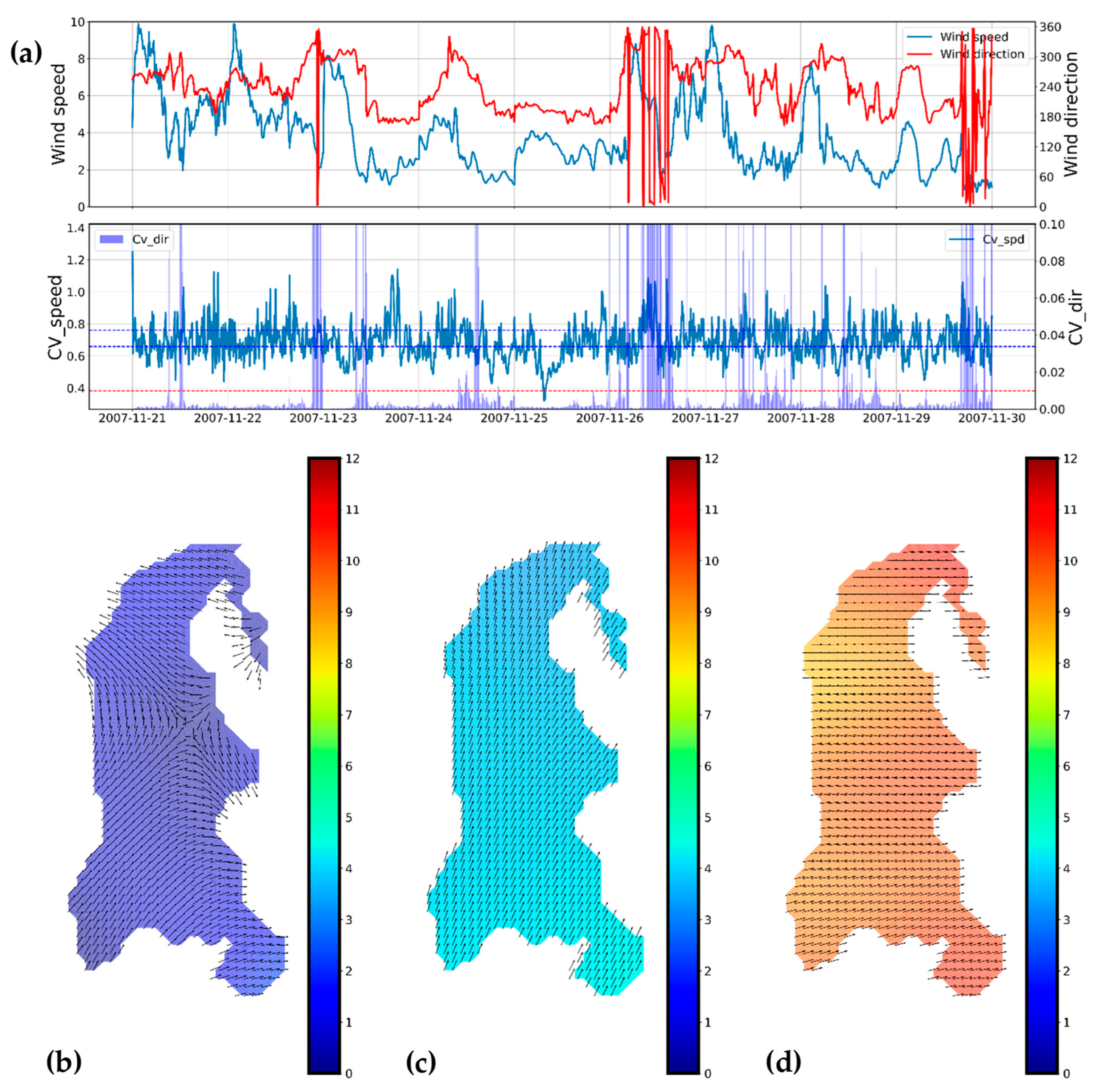
The spatial inhomogeneity levels of wind speed and direction were calculated with nine levels of the 2D mean filter (m = 9). The overall results are presented in (Figure 4a). The study period indicated general homogeneous wind direction in accordance with strong wind speed. Moreover, strong, and weak winds corresponded to low and high averaged coefficient of variance (Appendix B), scores, revealing an inverse relationship between the wind magnitude and the quantification score. According to a rough wind inhomogeneity estimation [40], values of less than 0.01 and less than 0.66 are considered spatially homogeneous, while values of higher than 0.01 and higher than 0.76 demonstrate spatial inhomogeneity. In addition to the inverse relationship mentioned above, moderate wind (3–5 m/s) illustrated an ambiguous pattern in spatial distribution. As a result, the complexity of spatial distribution could potentially signify the difference in the lake’s hydrodynamics. Based on the wind magnitude and the spatial inhomogeneity indicator, Figure 4b–d represent the spatial variations or spatial uniformity in wind. On the last day of the simulation (29 November 2007 23:50), very weak spatial wind (~1 m/s) produced insufficient momentum, disturbing the direction of the wind over the surface water body. Additionally, light air (~2 m/s) combined with moderate breeze (~4 m/s) (24 November 2007 15:00) formed a wind curl as a result of the shear stress differences in space. Figure 4c,d illustrated light (~4 m/s) to fresh breeze (~10 m/s), respectively. As we can see, near-spatial uniformity was noted in the wind over the lake’s surface. Therefore, we can assume a spatially uniform wind field during the strong wind periods, while the moderate wind-induced periods can alter the lake’s hydrodynamics due to the spatial variation of winds.
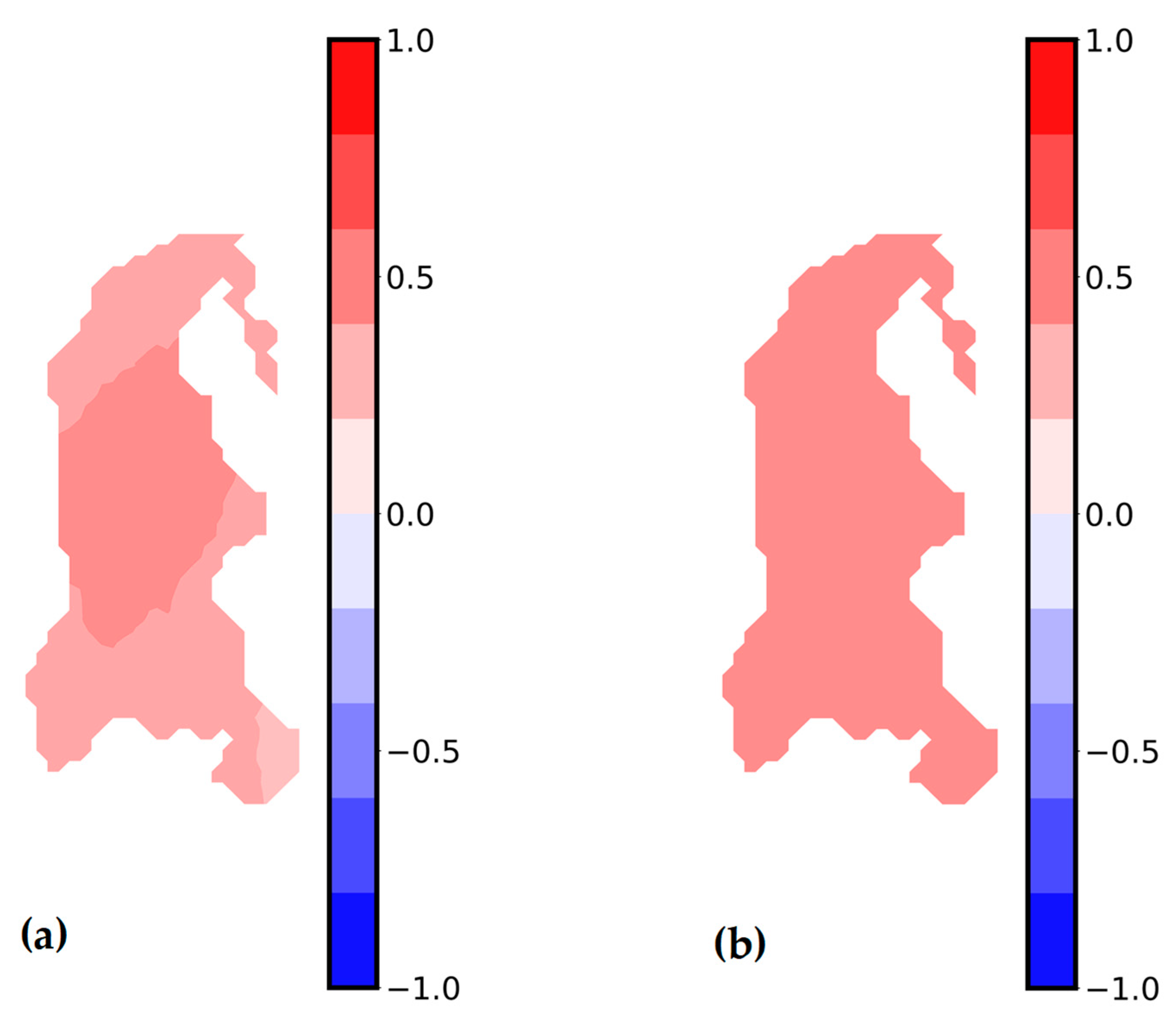
Pearson correlation coefficients were estimated in the 2D time series wind data between the central grid and its surrounding grids over the simulation period (Figure 5). Correlation coefficients were calculated using Equation (3). For the wind direction, temporal inhomogeneity exhibited an overall positively moderate correlation from the middle point to its nearby grids, while weaker relationships were located farther from the center grid (Figure 5a). Therefore, insignificant spatial wind similarity covered the entirety of Lake Abashiri. This could be explained by the spatially disturbed wind direction during weak-to-moderate wind periods. On the other hand, surprisingly, wind speed illustrated relatively spatially homogeneous correlation coefficients all over the area, with moderate correlation coefficients. In conclusion, wind speed represented acceptable similarity (~0.5) but wind direction illustrated higher spatial disturbance over the simulation period.
3.3. Surface Particle Transport and Tracer Transport
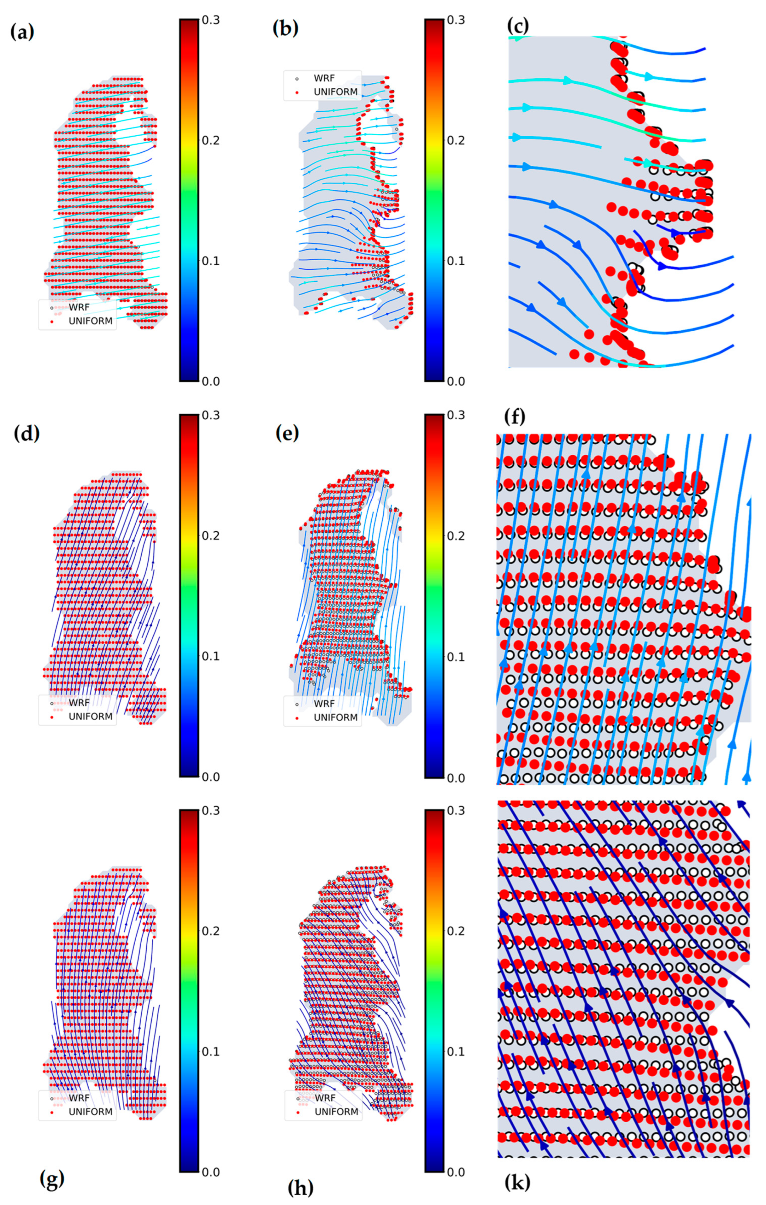
Figure 6 shows the numerical simulations of wind-induced surface particle transport. Theoretically, particles traveled unidirectionally following the wind direction under spatially uniform wind. This is consistent under strong and moderate wind speeds, which inversely correlate to the low . Figure 6c,f display a constant movement of particles following the water currents driven by the strong and moderate winds, respectively. Therefore, low generated translational motions in surface particles along the wind directions. In contrast to the strong wind, weak breezes generated the distinguishable motions of the water currents during a short time scale of the fundamental period, (8 h), because of the large and , showing the tendency of dispersing particles (Figure 6k). Compared to the spatial uniform wind, spatially distorted weak wind (~1 m/s) initiates a short distance of movement after the period. However, particles started to travel omnidirectionally after providing sufficient drag force, causing the particles to scatter in different directions (Figure 6k). This means that after a long period (>) of spatial variations in winds (large and ), the movement of surface particles would be far more different from that of spatially uniform wind.
Tracer mass transport was initially placed at the small estuary where the substances from the seaside were first provided in this lake. Figure 7 shows the concentration and distribution of the tracer under different wind conditions. Although the effects were relatively similar in both cases due to the prevailing wind direction, there were some discrepancies noted in the first few days of the simulation. For the first two days of strong prevailing NE wind, the tracer dispersion was mainly transferred to the estuary mount. As a result, the mass transport was blocked by the right-hand side boundary. The tracer was stirred up by the vertical circulation, which resulted in the tracer spreading over half of the water surface. Under uniform wind, the stable and homogeneous wind increased the concentration of tracer further south, while a lower concentration level was observed in the case of non-uniform wind (Figure 7b). The results of the inhomogeneous wind, which generated spatially disturbing water currents compared to that of spatially uniform wind, illustrated changes with less concentration in the southernmost part of the lake. By the end of the simulation, tracer mass transport was seen to be completely mixed up in the two wind cases, leaving no traits of a dominantly concentrated area.
3.4. Internal Seiche
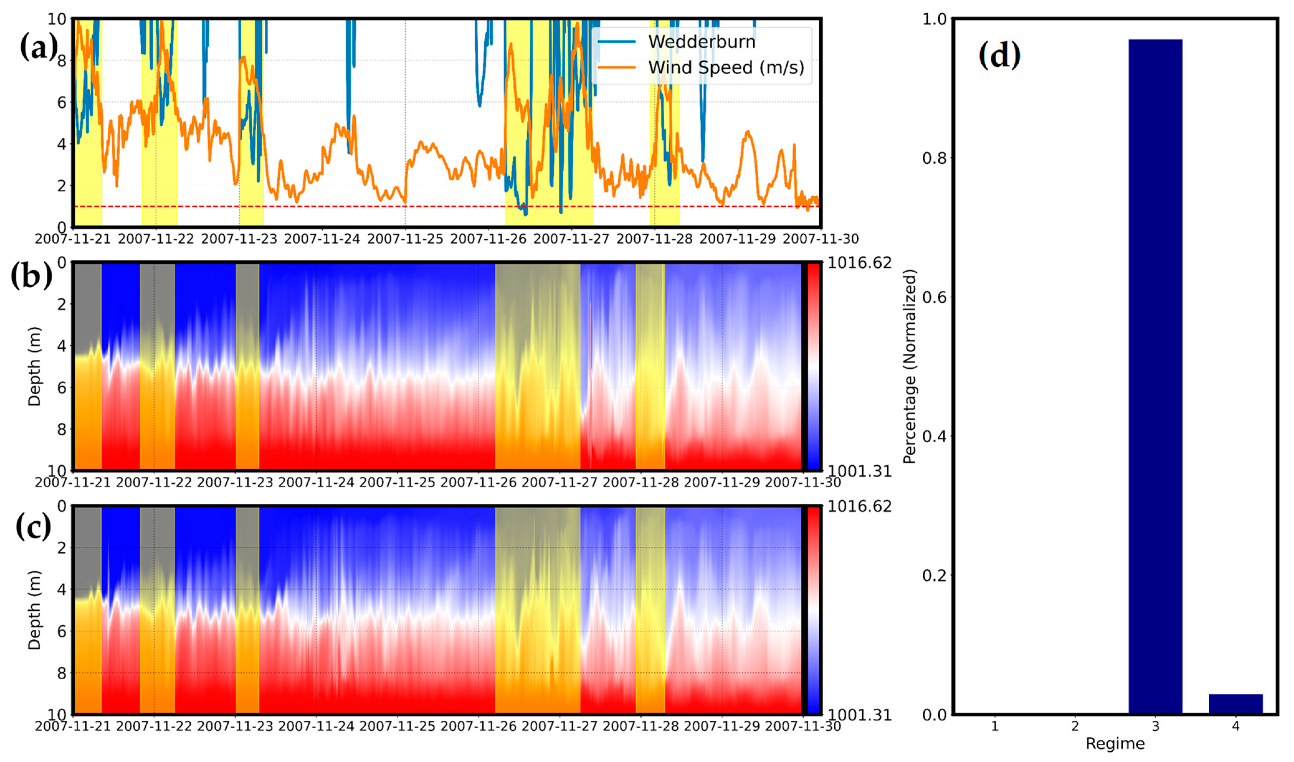
In general, the uniform and non-uniform wind shared similarities in inducing internal waves under the strongly stratified lake system (Figure 8). The depth of halocline computed under both wind cases did not present any complete upwelling under strong wind imposition. This was further confirmed by accessing the relationship between wind and the response of stratification (Figure 8c). There were roughly 96% of the total periods that are classified as “regime three” [43]. This indicated that the most prominent feature is internal seiching. Under this regime, strong wind durations are less than the entrainment time, illustrating the rare event of complete vertical mixing [43]. Regime four accounted for the remaining periods, showing the overall domination of buoyancy force. However, the complete dominance of regime three during the simulation period emphasized the importance of internal waves in this lake system.
A Wedderburn (W) (Figure 8a) number of 4 to 10 was often observed during the first period of strong prevailing NE wind force which gradually transferred energy and induced internal waves for approximately 5 days (Figure 8b). Strong oscillation was shown after the 26th and continued to highly fluctuate for roughly two days. This pattern was similar from the 28th onward. During this period, there was some time when W < 1 indicating potential mixing. This could explain why the resuspension events eventually happened under high wind speed [47]. However, the short periods of strong wind induced could not entirely mix up the strongly stratified lake system. After that, the imposition of weak-to-moderate wind did not generate enough energy, indicating the domination of buoyancy and damping effects.
The depth of the halocline in both wind cases under strong wind illustrated noteworthy features. On the first few days of the simulation period, both spatially uniform and non-uniform wind exhibited their similar features because of the strong wind speed and low and (Figure 4a). The minor discrepancies started to exhibit on the next few days under the effects of weak-to-moderate wind speeds. Between the 26th and 28th, strong wind imposed on lake displayed similarities in the high fluctuations following the notable Wedderburn numbers. According to Figure 8b,c, after the 28th, the buoyancy and damping effects were much higher than those produced by low wind speeds. It is also noted that more mixings were seen under the imposition of spatially uniform wind (Figure 8b). Therefore, the effects of low-to-moderate wind speed accompanied by high fluctuation in wind direction must not be neglected.
4. Discussion
4.1. The Differences in Surface Mass Transport and Water Current between Spatially Uniform Wind and Spatially Non-Uniform Wind
The weak and spatially inhomogeneous wind forcing generated the uneven water current and could explain the significant differences in the particle distributions (Figure 6) among three cases during the short time scale of , as shown in Figure 9.
Low and in the case of moderate to strong wind induced the water current to flow unidirectionally over the water surface. In addition to the high wind magnitudes, the wind direction did not change rapidly as it did in the weak wind condition (Figure 9a,b), which induced enough energy to push almost all the surface particles unidirectionally. This is consistent with the numerical simulation in [12]; the study illustrated that the horizontal transport of particles was stronger in winter Föhn due to the high and persistent magnitude of wind speed. As mentioned earlier, low values of and wind fields can indicate uniform wind fields. This can further reaffirm why wind speed is important and highly correlated with the wind direction as well as the water current.
On the other hand, in spatially non-uniform wind (Figure 9d), wind speeds were mostly below 2 m/s, and the low wind speed was often accompanied by omnidirectional wind direction [48], resulting in a disturbance of the movement of water current omnidirectionally across the lake. In contrast, spatially uniform wind (Figure 9c) produced a unidirectional water current in most parts of the lake, revealing the major differences in water current directions in both wind cases. Therefore, scattering effects would occur in the former wind case.
The assumptions of the flat bathymetry and the enclosed system, additionally, affirm that water-current curl (Figure 9d) can be formed under the imposition of spatial variations in wind due to the shear stress gradients where sheltering effects can be neglected in this lake [20]. A two-gyre circulation developed in Figure 9d, in which the clockwise gyre in the southern part coexisted with the counterclockwise gyre; meanwhile there was no such circulation under the strong wind condition. Depending on the lake size, this phenomenon is often observed when applying wind inhomogeneities as a governing factor [24]. Additionally, because Lake Abashiri is located in a flat and simple orography, the sheltering effects are minor, thus confirming the major effects of wind inhomogeneity. Based on the spatial distribution of water current (Figure 9), although the geometry of Lake Abashiri is simple, littoral zones in the south and at the middle generated clockwise flow, thus increasing the horizontal circulation (Figure 9d); meanwhile, this cannot be seen in spatially uniform wind conditions under the period of (Figure 9c). As mentioned earlier, based on the calculated and scores, the high values when moderate winds were observed would create wind curls due to the gradient. The uneven distribution of wind shear stress can be sufficiently important for understanding the movements of water currents as well as particulate organic matter (POM).
4.2. Correlation between Spatio-Temporal Indicators and Tracer Mass Transport
A strong and prevailing north-easterly wind (NE) was the main factor controlling the similar movement of the tracer down to the south of the lake on the first few days; the tracer was finally mixed up entirely at the end of simulation period (Figure 7). As the tracer was completely mixed up after nine days of simulation, the complex alteration in hydrodynamics might be difficult to observe. To overcome that issue, a tracer placed on the 27th of November revealed the noteworthiness of spatially varied wind imposition (Figure 7c). After one day, the tracer started reducing its concentration at the north boundary, while a higher concentration accumulated under non-uniform conditions and remained at the north of the lake. At the end of the simulation, concentrations remained higher in the case of spatial variations in wind, while the tracer concentration was fully mixed up with uniform wind.
Interestingly, the result obtained from the spatial variations in wind (Figure 7c) indicated that the movement of POM would transport it to the center of the lake, which is similar to the transportation of POM gathering at the center of the Tokyo Bay [25]. High moisture POM tends to accumulate at the center of the bay head [49,50]. Although the effects of wind curls and the assumptions of flat bathymetry in this study can be the factor producing the high concentrations at the lake center, real bathymetry can also increase the effect because it increases the water current velocity at the littoral zones. Further study is needed to understand the formation of positive and negative wind curl, and its effects on upwelling and downwelling under spatial variations in wind in combination with the real bathymetry.
4.3. Effects of Temporal and Spatial Frequencies of Winds to Internal Seiche
Overall, Figure 8 illustrates that the differences in internal waves of both wind cases were minor after nine days of the simulation. Noticeably, under strong wind during the first days of simulation (Figure 8), the height of the halocline responded comparably under both wind scenarios, wherein the differences as well as the major component causing the difference cannot be distinguished. To differentiate, the weak to strong wind-induced internal wave should be tested over a brief period. Simulations of internal waves within were conducted to understand the differences under both wind conditions.
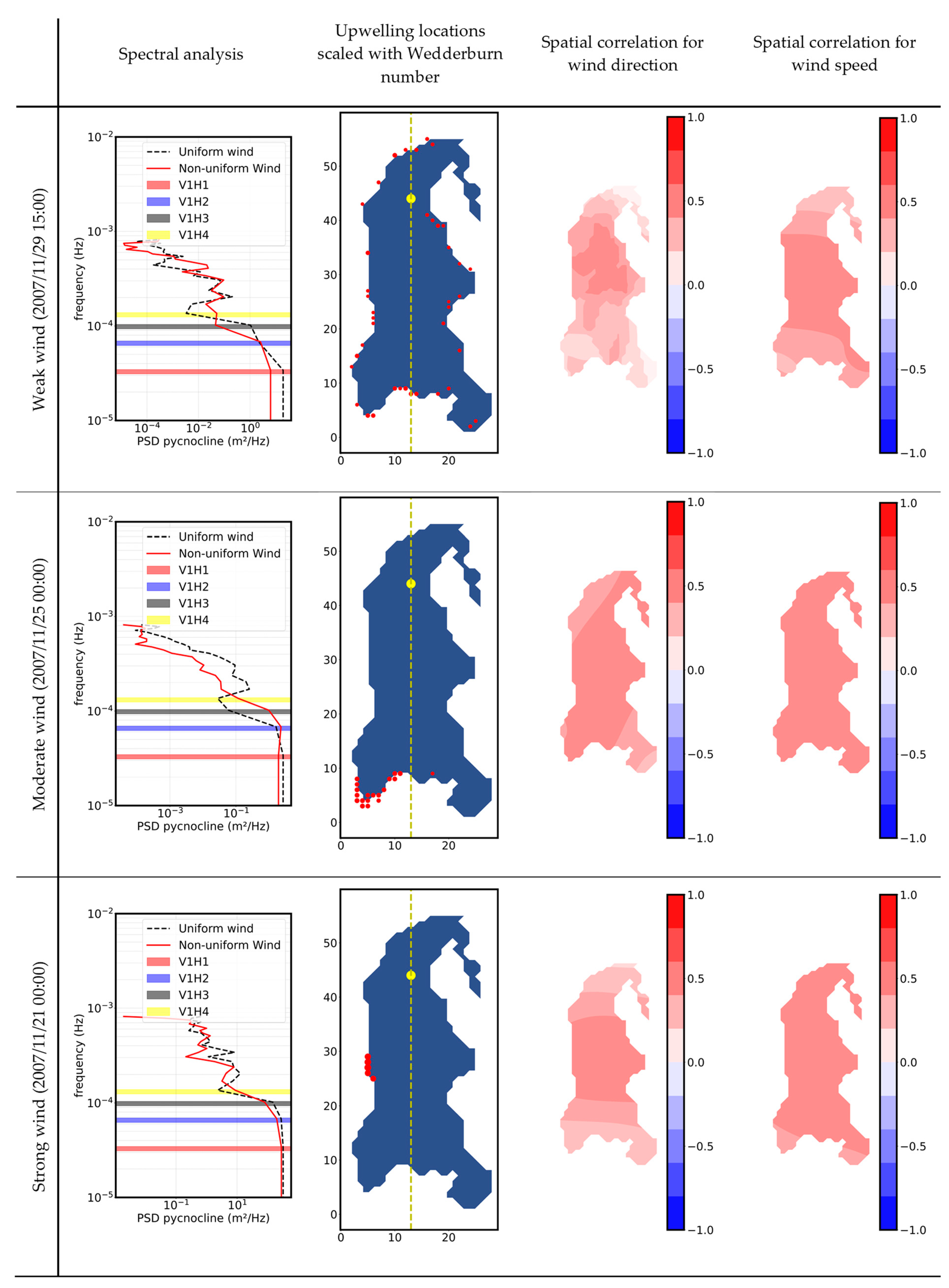
Figure 10 shows that the uneven distribution of wind direction was highlighted, with inverse correlation existing at southern part of the lake and a gradient from the center to the lake boundary in magnitude. Consequently, upwelling points were scattered, reducing the similar features of wind-induced internal wave. Considering the differences in spatial and temporal wind features, the results of spectral analysis generated a huge difference in PSD as well as frequency. While uniform wind coincides with V1H3 mode, non-uniform wind appeared to match to V1H2 mode. These alterations were obviously the main factors changing the behaviors of internal seiche in this system.
An eight-hour simulation of moderate wind (25 November 2007 00:00) indicated the overall stability of the lake’s system. The temporal correlation of wind speed and direction showed a reasonable similarity of both spatial uniformity and non-uniformity (Figure 10). The moderate wind featured North-East (NE) as the general prevailing wind, resulting in most of the upwelling locations being located at the south end of the lake. This feature indicated a similar internal seiche in V1H2 mode, whereas both wind-induced internal wave cases disagreed in V1H3 mode, with a lower PSD in non-uniform wind compared to that of uniform wind. In addition, lower wind speed correlated to the PSD generated by the internal waves.
Finally, for the strong wind (~10 m/s), winds were predominantly easterly (E) during the period of (). This could be seen from the upwelling locations accumulated at the western end of the lake boundary. Spectral analysis revealed that the prevailing wind (E) of spatially uniform and non-uniform wind excited internal waves with relatively similar power spectral densities at modes V1H1, V1H2, and V1H3. However, the numerical model did not match the mode V1H4. Moreover, both wind cases excited a similar PSD of internal waves, which reaffirms the similarity in both spatial uniformity and nonuniformity under strong wind fields.
5. Conclusions
The study aimed to investigate the responses of the hydrodynamics of a lake under both spatially uniform and spatially non-uniform wind fields. Lake Abashiri was selected as the field, and the flat bottom of the lake was assumed for the analysis in order to focus on the effect of wind nonuniformity on the lake response. The realistic nonuniform weather was generated by the weather research and forecasting model with four level nesting grids over the area. To quantify the level of inhomogeneity of wind speed and wind direction, the wind products from WRF were then analyzed based on a 2D mean filter. Three of the lake’s physical responses, including surface particle transport, tracer tracking, and internal waves, were examined under the different wind conditions. The analysis highlighted the key factors that effect changes when applying different wind scenarios.
Firstly, strong wind corresponding to a low level of variances both for wind speed and direction, and , provided sufficient momentum to unidirectionally push the surface particles horizontally to the shoreline within the fundamental period of this stratified lake, . On the other hand, wind curl was formed under the imposition of a weak-to-moderate wind field of high values of variance both in speed and direction. The surface particles moved only short distances but not unidirectionally, so they would be transported differently for the succeeding phase in the case of the uniform wind.
Secondly, when appropriately placing the tracer mass transport under wind of high variances, the possible effects of wind non-uniformity could be observed in the transport process in the POM concentration at the bay head of Lake Abashiri. Particularly, in the present study, a much higher concentration was seen in the more realistic wind condition, while a smaller concentration was seen in the case of spatially uniform wind.
Finally, the internal wave spectral analysis in both wind cases showed comparably similar patterns when considering the whole simulated period. Furthermore, the potential mixing, as defined by the Wedderburn number, showed that strong wind provided enough energy to fluctuate and potentially upwell the downwind along the fetch length. However, the system could not be mixed; this was probably due to the short duration of the strong wind and the assumption of uniform bathymetry. The analysis under the shorter time scale (), revealed that the weaker the wind, the larger difference in power spectral density. This further elucidated the importance of weak-to-moderate wind effects on lake hydrodynamics.
This study emphasized the significant differences between spatially uniform and spatially non-uniform winds when comparing their interactions with surface mass transport, tracer tracking, and internal waves, excluding the effects of the bathymetry. Although it is important to consider the effects of bathymetry, they can, together with spatially non-uniform wind, alter and contribute to the complexity of lake hydrodynamics. As a result, future studies will include bathymetry effects to further analyze the sensitivity of lake hydrodynamics, coupled with spatial and temporal variations in wind.
Author Contributions
Conceptualization, H.N.L. and T.S.; Data curation, H.N.L.; Formal analysis, H.N.L.; Methodology, H.N.L.; Resources, T.S. and K.N.; Supervision, T.S.; Validation, T.S.; Visualization, H.N.L.; Writing—original draft, H.N.L.; Writing—review and editing, T.S. and K.N. All authors have read and agreed to the published version of the manuscript.
Funding
This research received no external funding.
Institutional Review Board Statement
Not applicable.
Informed Consent Statement
Not applicable.
Data Availability Statement
Not applicable.
Acknowledgments
The first author would like to give his sincere gratitude to the Japanese Government (Monbukagakusho) Scholarship for the grant for his Ph.D studies at the Tokyo Metropolitan University.
Conflicts of Interest
The authors declare no conflict of interest.
Appendix A. Fantom-Refined Model Description
The Fantom-Refined model applies 3-D Navier–Stokes equations with incompressible and Boussinesq approximation
subject to incompressibility,
where , , and are the velocities in the , , and directions, respectively. is the pressure, is the reference density, is the density, is the Coriolis coefficient, is the latitude, is the angular velocity of the earth, and are the horizontal and vertical eddy viscosity coefficients. The depth-averaged continuity equation, which is given hereafter, governs the evolution of the free surface.
where is the free-surface height and is the bathymetric depth. The transport equations for temperature and salinity are given by
where is the temperature, is the salinity, and are the horizontal and vertical eddy diffusion coefficients.
A collocated finite-volume approach was used to discretize the governing equations [51,52]. For explicit terms such as advection of momentum, horizontal diffusion, and Coriolis force, the second-order Adams–Bashforth technique was used to discretize temporal derivatives [53]. Surface elevation and vertical momentum and scalar diffusion were estimated semi-implicitly using the TRIM technique, a second-order theta approach [54]. The advection terms were spatially discretized for the momentum and scalars using the third-order ULTIMATE-QUICKEST scheme [55], while the horizontal diffusion terms were discretized using the second-order central differencing scheme.
Appendix B. Spatial Variations in Wind Quantification
To observe the spatial consistency of the two-dimension dataset, the discrepancies in subsequent increments in size selection for both wind speed and direction were calculated as:
where and are the filtered images with size +1 and , respectively. This filtering technique will reduce the horizontal resolution of the array size. However, no padding is applied to fill the surrounding array to prevent the model from being biased. Next, the spatial variation in wind speed is described as follows:
where is the coefficient of variance of spatial wind speed, is the population size, is the value of the difference between each filter of the wind speed in each grid, is the mean wind speed. For the complexity in the wind direction, is estimated based on Yamartino [56].
where , , , and , is the value of the difference between each filter of the wind direction in each grid. Values of and are then averaged based on the number of layers () being filtered, based on the proposed method of [40].
References
- Ueda, S.; Kondo, K.; Chikuchi, Y. Effects of the halocline on water quality and phytoplankton composition in a shallow brackish lake (Lake Obuchi, Japan). Limnology 2005, 6, 149–160. [Google Scholar] [CrossRef]
- Lougee, L.A.; Bollens, S.M.; Avent, S.R. The effects of haloclines on the vertical distribution and migration of zooplankton. J. Exp. Mach. Biol. Ecol. 2002, 278, 111–134. [Google Scholar] [CrossRef]
- Gantzer, P.A.; Bryant, L.D.; Little, J.C. Controlling soluble iron and manganese in water-supply reservoir using hypolimnetic oxygenation. Water Res. 2009, 43, 1285–1294. [Google Scholar] [CrossRef] [PubMed]
- Yuk, J.; Aoki, S. Effect of Wind and Rainfall on Water Exchange in a Stratified Estuary. Estuary Coasts 2009, 32, 88–99. [Google Scholar] [CrossRef]
- Yao, J.; Li, Y.; Zhang, D.; Zhang, Q.; Tao, J. Wind effects on hydrodynamics and implications for ecology in a hydraulically dominated river-lake floodplain system: Poyang Lake. J. Hydrol. 2019, 571, 103–113. [Google Scholar] [CrossRef]
- Rafael, C.B. Wind-Induced Internal Waves in Closed Basins: A Laboratory Experiment and Field Study. Master’s Thesis, Universidade Federal Do Parana, Curitiba, Brazil, 2018. [Google Scholar]
- Maruya, Y.; Nakayama, K.; Shintani, T.; Yonemoto, M. Evaluation of entrainment velocity induced by wind stress in a two-layer system. Hydrol. Res. Lett. 2010, 4, 70–74. [Google Scholar] [CrossRef]
- Ishikawa, T.; Tanaka, M. Diurnal stratification and its effects on wind-induced currents and water qualities in Lake Kasumigaura, Japan. J. Hydraul. Res. 1993, 31, 307–322. [Google Scholar] [CrossRef]
- Paerl, H.W.; Hall, N.S.; Calandrino, E.S. Controlling harmful cyanobacterial blooms in a world experiencing anthropogenic and climatic-induced change. Sci. Total Environ. 2011, 409, 1739–1745. [Google Scholar] [CrossRef]
- Kopasakis, K.; Laspidou, C.; Spiliotopoulos, M.; Kofinas, D.; Mellios, N. Numerical Investigation of Wind Driven Circulation and Horizontal Dispersion in the Surface Layer of a Re-flooded Shallow Lake. Environ. Process. 2016, 3, 693–710. [Google Scholar] [CrossRef]
- Sprules, W.G.; Cyr, H.; Menza, C.W. Multiscale effects of wind-induced hydrodynamics on lake plankton distribution. Limnol. Oceanogr. 2022, 67, 1631–1646. [Google Scholar] [CrossRef]
- Amadori, M.; Piccolroaz, S.; Giovannini, L.; Zardi, D.; Toffolon, M. Wind variability and Earth’s rotation as drivers of transport in a deep, elongated subalpine lake: The case of Lake Garda. J. Limnol. 2018, 77, 505–521. [Google Scholar] [CrossRef]
- Schwab, D.J.; Beletsky, D. Relative effects of wind stress curl, topography, and stratification on large-scale circulation in Laka Michigan. J. Geophys. Res. Oceans 2003, 108, 3044. [Google Scholar] [CrossRef]
- Santo, M.A.; Toffolon, M.; Zanier, G.; Giovannini, L.; Armenio, V. Large eddy simulation (LES) of wind-driven circulation in a peri-alpine lake: Detection of turbulent structures and implications of a complex surrounding orography. J. Geophys. Res. Oceans 2017, 122, 4704–4722. [Google Scholar] [CrossRef]
- Valerio, G.; Pilotti, M.; Marti, C.L.; Imberger, J.R. The structure of basin-scale internal waves in a stratified lake in response to lake bathymetry and wind spatial and temporal distribution: Lake Iseo, Italy. Limnol. Oceanogr. 2012, 57, 772–786. [Google Scholar] [CrossRef]
- Amadori, M.; Giovannini, L.; Toffolon, M.; Piccolroaz, S.; Zardi, D.; Bresciani, M.; Giardino, C.; Luciani, G.; Kliphuis, M.; van Haren, H.; et al. Multi-scale evaluation of a 3D lake model forced by an atmospheric model against standard monitoring data. Environ. Model. Softw. 2021, 139, 105017. [Google Scholar] [CrossRef]
- Li, C.; Odermatt, D.; Bouffard, D.; Wüest, A.; Kohn, T. Coupling remote sensing and particle tracking to estimate trajectories in large water bodies. Int. J. Appl. Earth Obs. Geoinf. 2022, 110, 102809. [Google Scholar] [CrossRef]
- Okely, P.; Imberger, J.R.; Antenucci, J.P. Processes affecting horizontal mixing and dispersion in Winam Gulf, Lake Victoria. Limnol. Oceanogr. 2010, 55, 1865–1880. [Google Scholar] [CrossRef]
- Mao, M.; Xia, M. Particle Dynamics in the Nearshore of Lake Michigan Revealed by an Observation-Modeling System. J. Geophys. Res. Oceans 2020, 125, e2019JC015765. [Google Scholar] [CrossRef]
- Liu, S. Wind Driven Circulation in Large Shallow Lakes. Doctoral Thesis, Delft University of Technology, Delft, The Netherlands, 2020. [Google Scholar]
- Cimatoribus, A.A.; Lemmin, U.; Barry, D.A. Tracking Lagrangian transport in Lake Geneva: A 3D numerical modeling investigation. Limnol. Oceanogr. 2019, 64, 1252–1269. [Google Scholar] [CrossRef]
- Laval, B.; Imberger, J.; Hodges, B.R.; Stocker, R. Modelling circulation in lakes: Spatial and temporal variations. Limnol. Oceanogr. 2003, 48, 983–994. [Google Scholar] [CrossRef] [Green Version]
- Podsetchine, V.; Schernewski, G. The Influence of spatial wind inhomogeneity on flow patterns in a small lake. Water Res. 1999, 33, 3348–3356. [Google Scholar] [CrossRef]
- Rubbert, S.; Köngeter, J. Measurements and three-dimensional simulations of flow in a shallow reservoir subject to small-scale wind field inhomogeneities induced by sheltering. Aquat. Sci. 2005, 67, 104–121. [Google Scholar] [CrossRef]
- Nakayama, K.; Shintani, T.; Shimizu, K.; Okada, T.; Hinata, H.; Komai, K. Horizontal and residual circulations driven by wind stress curl in Tokyo Bay. J. Geophys. Res. Oceans 2014, 119, 1977–1992. [Google Scholar] [CrossRef]
- Chikita, K. Dynamic behaviours of anoxic saline water in Lake Abashiri, Hokkaido, Japan. Hydrol. Process. 2000, 14, 557–574. [Google Scholar] [CrossRef]
- Maruya, Y.; Nakayama, K.; Sasaki, M.; Komai, K. Effect of dissolved oxygen on methane production from bottom sediment in a eutrophic stratified lake. J. Environ. Sci. 2023, 125, 61–72. [Google Scholar] [CrossRef] [PubMed]
- Japan Meteorological Agency. Japan Meteorological Agency|AMeDAS. Available online: https://www.jma.go.jp (accessed on 10 October 2022).
- User’s Guides for the Advanced Research WRF (ARW) Modeling System, Version 3. Available online: https:/www2.mmm.ucar.edu/wrf/users/docs/user_guide_V3/contents.html (accessed on 31 May 2022).
- Copernicus Climate Data Store. Available online: https://cds.climate.copernicus.eu/cdsapp (accessed on 10 October 2022).
- Hersbach, H.; Bell, B.; Berrisford, P.; Hirahara, S.; Horányi, A.; Muñoz-Sabater, J.; Nicolas, J.; Peubey, C.; Radu, R.; Schepers, D.; et al. The ERA5 global reanalysis. Q. J. R. Meteorol. Soc. 2020, 146, 1999–2049. [Google Scholar] [CrossRef]
- Solbakken, K.; Birkelund, Y.; Samuelsen, E.M. Evaluation of surface wind using WRF in complex terrain: Atmospheric input data and grid spacing. Environ. Model. Softw. 2021, 145, 105182. [Google Scholar] [CrossRef]
- Olauson, J. ERA5: The new champion of wind power modelling? Renew. Energy 2018, 126, 322–331. [Google Scholar] [CrossRef]
- Ramon, J.; Lledó, L.; Torralba, V.; Soret, A.; Doblas-Reyes, F.J. What global reanalysis best represents near-surface winds? Q. J. R. Meteorol. Soc. 2019, 145, 3236–3251. [Google Scholar] [CrossRef]
- Monin, A.S.; Obukhov, A.M. Basic Laws of Turbulent Mixing in the Surface Layer of the Atmosphere. Contrib. Geophys. Inst. Acad. Sci. USSR 1954, 24, 163–187. [Google Scholar]
- Global Map Japan. Available online: https://www.gsi.go.jp/kankyochiri/gm_japan_e.html (accessed on 10 October 2022).
- Shintani, T. An unstructured-cartesian hydrodynamic simulator with local mesh refinement technique. J. JSCE (Hydraul. Eng.) 2017, 73, 967–972. [Google Scholar] [CrossRef] [Green Version]
- Veerapaga, N.; Azhikodan, G.; Shintani, T.; Iwamoto, N.; Yokoyama, K. A three-dimensional environmental hydrodynamic model, Fantom-Refined: Validation and application for saltwater intrusion in a meso-macrotidal estuary. Ocean Model. 2019, 141, 101425. [Google Scholar] [CrossRef]
- Kondo, J. Air-sea bulk transfer coefficients in diabatic conditions. Bound.-Layer Meteorol. 1975, 9, 91–112. [Google Scholar] [CrossRef]
- Hieu, N.L.; Shintani, T. Numerical Investigation on Inhomogeneous Wind and Its Effects to Mass Transport. J. JSCE 2022, in press. [Google Scholar]
- Shintani, T.; de la Fuente, A.; de la Fuente, A.; Niño, Y.; Imberger, J. Generalizations of the Wedderburn number: Parameterizing upwelling in stratified lakes. Limnol. Oceanogr. 2010, 55, 1377–1389. [Google Scholar] [CrossRef]
- Mortimer, C.H. Water movements in lakes during summer stratification; evidence from the distribution of temperature in Windermere. Philos. Trans. R. Soc. Lond. Ser. B Biol. Sci. 1952, 236, 355–398. [Google Scholar]
- Spigel, R.H.; Imberger, J. The classification of Mixed-Layer Dynamics of Lakes of Small to Medium Size. J. Phys. Oceanogr. 1980, 10, 1104–1121. [Google Scholar] [CrossRef]
- Simmons, H.; Chang, M.H.; Chang, Y.T.; Chao, S.Y.; Fringer, O.; Jackson, C.; Ko, D.S. Modeling and Prediction of Internal Waves in the South China Sea. Oceanography 2011, 24, 88–99. [Google Scholar] [CrossRef]
- Lin, H. Hydropedology: Synergistic integration of soil science and hydrology. Choice Rev. Online 2013, 50, 4450–4451. [Google Scholar]
- Pannard, A.; Beisner, B.E.; Bird, D.F.; Braun, J.; Planas, D.; Bormans, M. Recurrent internal waves in a small lake: Potential ecological consequences for metalimnetic phytoplankton populations. Limnol. Ocean. Fluids Environ. 2011, 1, 91–109. [Google Scholar] [CrossRef]
- Rao, Y.R.; Schwab, D.J. Transport and Mixing between the Coastal and Offshore Waters in the Great Lakes: A Review. J. Great Lakes Res. 2007, 33, 202–218. [Google Scholar] [CrossRef]
- Jiménez, P.A.; Dudhia, J. On the Ability of the WRF Model to Reproduce the Surface Wind Direction over Complex Terrain. J. Appl. Meteorol. Climatol. 2013, 52, 1610–1617. [Google Scholar] [CrossRef]
- Preston, J.M.; Collins, W.T. Bottom classification in very shallow water by high-speed data acquisition. In Proceedings of the Oceans 2000 MTS/IEEE Conference and Exhibition, Providence, RI, USA, 11–14 September 2000; Volume 2, pp. 1277–1282. [Google Scholar]
- Nakayama, K.; Okada, T.; Nomura, M. Mechanism responsible for fortnightly modulations in estuary circulation in Tokyo Bay. Estuar. Coast. Shelf Sci. 2005, 64, 459–466. [Google Scholar] [CrossRef]
- Ferziger, J.H.; Peric, M. Computational Methods for Fluid Dynamics, 3rd ed.; Springer: Berlin/Heidelberg, Germany, 2002. [Google Scholar]
- Perot, B. Conservation Properties of Unstructured Staggered Mesh Schemes. J. Comput. Phys. 2000, 159, 58–59. [Google Scholar] [CrossRef] [Green Version]
- Zang, Y.; Street, R.L.; Koseff, J.R. A Non-staggered Grid, Fractional Step Method for Time-Dependent Incompressible Navier-Stokes Equations in Curvilinear Coordinates. J. Comput. Phys. 1994, 114, 18–33. [Google Scholar] [CrossRef]
- Casulli, V. A semi-implicit finite difference method for non-hydrostatic, free-surface flows. Int. J. Numer. Methods Fluids 1999, 30, 425–440. [Google Scholar] [CrossRef]
- Leonard, B. The ULTIMATE conservative difference scheme applied to unsteady one-dimensional advection. Comput. Methods Appl. Mech. Eng. 1991, 88, 17–74. [Google Scholar] [CrossRef]
- Yamartino, R.J. A Comparison of Several “Single-Pass” Estimators of the Standard Deviation of Wind Direction. J. Clim. Appl. Climatol. 1984, 23, 1362–1366. [Google Scholar] [CrossRef]
Figure 1.
Maps of (a) Lake Abashiri with four nesting domains, (b) the station location, and (c) Lake Abashiri bathymetry.
Figure 1.
Maps of (a) Lake Abashiri with four nesting domains, (b) the station location, and (c) Lake Abashiri bathymetry.

Figure 2.
Fantom-Refined 3D configurations; (a) (square boxes) horizontal LMR mesh resolution, and (b) (black dashed line) vertical resolution along the fetch length. Blue dashed line is the water surface and the red connected dotted line is the side view bathymetry of the red line drawn in (a).
Figure 2.
Fantom-Refined 3D configurations; (a) (square boxes) horizontal LMR mesh resolution, and (b) (black dashed line) vertical resolution along the fetch length. Blue dashed line is the water surface and the red connected dotted line is the side view bathymetry of the red line drawn in (a).

Figure 3.
Validation in wind speed and wind direction between WRF and station data (Tokoro). (a) Validation in wind speed, (b) WRF model wind direction, and (c) Station wind direction.
Figure 3.
Validation in wind speed and wind direction between WRF and station data (Tokoro). (a) Validation in wind speed, (b) WRF model wind direction, and (c) Station wind direction.

Figure 4.
Maps of (a) Wind speed and direction inhomogeneity, (b) weak wind with high = 0.1, = 0.615 (29 November 2007 23:50), (c) moderate wind with high = 0.0014, = 0.863 (25 November 2007 04:00), (d) strong wind with low = 0.001, = 0.624 (21 November 2007 01:30).
Figure 4.
Maps of (a) Wind speed and direction inhomogeneity, (b) weak wind with high = 0.1, = 0.615 (29 November 2007 23:50), (c) moderate wind with high = 0.0014, = 0.863 (25 November 2007 04:00), (d) strong wind with low = 0.001, = 0.624 (21 November 2007 01:30).

Figure 5.
Maps of (a) correlation of wind direction between the center grid and the surrounding grids, (b) correlation of wind speed between the center grid and the surrounding grids.
Figure 5.
Maps of (a) correlation of wind direction between the center grid and the surrounding grids, (b) correlation of wind speed between the center grid and the surrounding grids.

Figure 6.
Every twenty minutes of surface particle movement and current vectors of eight hours’ simulation, starting from 21 November 2007 00:00 (a); 25 November 2007 00:00 (d); and 29 November 2007 23:00 (g) to 21 November 2007 01:30 (b); 25 November 2007 00:00 (e); and 29 November 2007 23:50 (h), respectively. (c,f,k) are the zoom in of (b,e,h).

Figure 7.
Simulations of (a) (21 November 2007 00:00) and (b) (23 November 2007 23:00) in which tracer mass transport was placed at the beginning of the simulation, (c) (30 November 2007 00:00) where tracer was placed after the 27th onward.
Figure 7.
Simulations of (a) (21 November 2007 00:00) and (b) (23 November 2007 23:00) in which tracer mass transport was placed at the beginning of the simulation, (c) (30 November 2007 00:00) where tracer was placed after the 27th onward.

Figure 8.
Mixing condition (a) wind speed and Wedderburn number, (b) depth of density difference excited by uniform wind, (c) depth of density difference excited by non-uniform wind, and (d) normalized percentage of the four regimes.
Figure 8.
Mixing condition (a) wind speed and Wedderburn number, (b) depth of density difference excited by uniform wind, (c) depth of density difference excited by non-uniform wind, and (d) normalized percentage of the four regimes.

Figure 9.
Vectors of water currents; (a) spatially uniform wind with strong wind magnitudes, (b) spatially non-uniform wind with strong wind magnitudes, (c) spatially uniform wind with low magnitudes, and (d) spatially non-uniform wind with low wind magnitudes. All pairs of simulation are at the same time.

Figure 10.
Statistical analysis of wind-induced internal seiche at a certain time of interest; yellow dash line is the fetch length, yellow dots on upwelling locations scaled with Wedderburn numbers are the point taken for calculating internal waves.
Figure 10.
Statistical analysis of wind-induced internal seiche at a certain time of interest; yellow dash line is the fetch length, yellow dots on upwelling locations scaled with Wedderburn numbers are the point taken for calculating internal waves.


Table 1.
Weather research and forecasting model configurations.
| Domains | Domain 1 | Domain 2 | Domain 3 | Domain 4 |
|---|---|---|---|---|
| Resolution | 10 km × 10 km | 3.3 km × 3.3 km | 1.1 km × 1.1 km | 333 m × 333 m |
| No. of grid points | 200 × 200 | 190 × 190 | 178 × 178 | 166 × 166 |
| Microphysics | WSM3 | WSM3 | WSM3 | WSM3 |
| Longwave radiation | RRTM | RRTM | RRTM | RRTM |
| Shortwave radiation | Dudhia | Dudhia | Dudhia | Dudhia |
| Cumulus parameterization | Kain–Fritsch | Kain–Fritsch | Kain–Fritsch | None |
| Land-surface option | Noah-MP | Noah-MP | Noah-MP | Noah-MP |
| Surface layer option | Monin–Obukhov | Monin–Obukhov | Monin–Obukhov | Monin–Obukhov |
| Planetary boundary layer | Mellor–Yamada–Janjic | Mellor–Yamada–Janjic | Mellor–Yamada–Janjic | Mellor–Yamada–Janjic |
Table 2.
Fantom simulation durations setup. For every hour of time increment, the simulations of surface particle transports and internal seiches were reset every 8 h ( for the entire 9 days of the simulation. Tracer transport and another case of internal seiche were simulated with no reset for the entire 9 days of the simulation.
| Duration of Simulation | Time Steps | ||
|---|---|---|---|
| Spatial Uniformity | Spatial Variations | ||
| Surface particle transports | (8 h) | (8 h) | 10 s |
| Tracer transport | 9 days (tracer was placed at the 21st) | 9 days (tracer was placed at the 27th) | 10 s |
| Internal seiche | 9 days and (8 h) | 9 days and (8 h) | 10 s |
Disclaimer/Publisher’s Note: The statements, opinions and data contained in all publications are solely those of the individual author(s) and contributor(s) and not of MDPI and/or the editor(s). MDPI and/or the editor(s) disclaim responsibility for any injury to people or property resulting from any ideas, methods, instructions or products referred to in the content. |
© 2023 by the authors. Licensee MDPI, Basel, Switzerland. This article is an open access article distributed under the terms and conditions of the Creative Commons Attribution (CC BY) license (https://creativecommons.org/licenses/by/4.0/).
Share and Cite
MDPI and ACS Style
Le, H.N.; Shintani, T.; Nakayama, K. A Detailed Analysis on Hydrodynamic Response of a Highly Stratified Lake to Spatio-Temporally Varying Wind Field. Water 2023, 15, 565. https://doi.org/10.3390/w15030565
AMA Style
Le HN, Shintani T, Nakayama K. A Detailed Analysis on Hydrodynamic Response of a Highly Stratified Lake to Spatio-Temporally Varying Wind Field. Water. 2023; 15(3):565. https://doi.org/10.3390/w15030565
Chicago/Turabian StyleLe, Hieu Ngoc, Tetsuya Shintani, and Keisuke Nakayama. 2023. "A Detailed Analysis on Hydrodynamic Response of a Highly Stratified Lake to Spatio-Temporally Varying Wind Field" Water 15, no. 3: 565. https://doi.org/10.3390/w15030565
Note that from the first issue of 2016, this journal uses article numbers instead of page numbers. See further details here.