
A Review of Hydrodynamic and Machine Learning Approaches for Flood Inundation Modeling
by
 ,
,
Fazlul Karim
1,*, 
Mohammed Ali Armin
2,
David Ahmedt-Aristizabal
2,
Lachlan Tychsen-Smith
2 and
Lars Petersson
2,3 1
Managing Water Ecosystem Group, CSIRO Environment, Commonwealth Scientific and Industrial Research Organisation, Canberra 2601, Australia
2
Imaging and Computer Vision Group, CSIRO Data61, Canberra 2601, Australia
3
Machine Learning and Artificial Intelligence Future Science Platform, CSIRO Data61, Canberra 2601, Australia
*
Author to whom correspondence should be addressed.
Water 2023, 15(3), 566; https://doi.org/10.3390/w15030566
Submission received: 19 December 2022
/
Revised: 29 January 2023
/
Accepted: 30 January 2023
/
Published: 1 February 2023
(This article belongs to the Special Issue Advances in Flood Frequency and Inundation Modeling: Application of Statistical, Hydrodynamic, Remote Sensing, and Machine Learning Tools)
Abstract
:Machine learning (also called data-driven) methods have become popular in modeling flood inundations across river basins. Among data-driven methods, traditional machine learning (ML) approaches are widely used to model flood events, and recently deep learning (DL) approaches have gained more attention across the world. In this paper, we reviewed recently published literature on ML and DL applications for flood modeling for various hydrologic and catchment characteristics. Our extensive literature review shows that DL models produce better accuracy compared to traditional approaches. Unlike physically based models, ML/DL models suffer from the lack of using expert knowledge in modeling flood events. Apart from challenges in implementing a uniform modeling approach across river basins, the lack of benchmark data to evaluate model performance is a limiting factor for developing efficient ML/DL models for flood inundation modeling.
1. Introduction
Machine learning algorithms including traditional machine learning and more advanced deep learning models, have shown promising results for flood inundation modeling. Very recently, Bentivoglio et al. [1] reviewed the application of deep learning models for flood inundation modeling. They summarized the main challenges related to application of DL models as generalization ability, and modeling complicated interactions in flood events. Sit et al. [2] covered applications of DL models on a broad range of events including floods and weather forecasting. They concluded that because rainfall and runoff are both time series data, recurrent neural network (RNN) models are among the best suited for these events. They also highlighted the lack of a well curated dataset in the water modeling fields. Mudashiru et al. [3] reviewed the application of ML models to flood hazard maps and determined that uncertainty quantification is a limitation of ML. Ghorpade et al. [4] reviewed five papers and compared traditional ML and DL methods. They highlighted the effects of data (e.g., water flow, rain fall and humidity) and superiority of DL models for flood modeling. Mosavi et al. [5] reviewed several papers that used ML methods to estimate flood inundation, and investigated the robustness, effectiveness, accuracy, and speed of these models. As a result, they introduced the most promising prediction methods for both long- and short-term flood events.
Although these papers provide comprehensive information on ML and DL models, their focus was only ML or DL models. In this work, we reviewed physically based models used to generate flood inundation data for ML models and provided technical information about both ML and DL models and then surveyed papers that applied these models to predict flood events. Further, we discuss the strengths and weaknesses of such data-driven methods (e.g., ML, DL) to model flood events and describe challenges and missing technologies that can be explored by the community to boost speed and performance of flood prediction. Table 1 highlights the differences between our review and similar existing surveys.
Our paper is organized as follows: In Section 2, we briefly describe the common hydrodynamic, machine learning and deep learning methods used in this research field. Section 3 summarizes the formulation of traditional and DL methods and application of these methods for flood inundation modeling along with a review over datasets. We organize publications according to traditional ML and more advanced DL approaches. Section 4 highlights the strength and limitations of current methods and explains open research challenges. Finally, key findings of this review are summarized in Section 5.
2. Overview of Methods
2.1. Hydrodynamic Models
Hydrodynamic (HD) models have been used for several decades to describe the dynamics of flood inundation systems [6,7,8]. Based on the complexity of the river-floodplain network in question and data availability for model configuration and calibration, one can select a simple (e.g., one dimensional, 1D), or more complex two dimensional (2D) or coupled 1D and 2D model [6,9]. The 1D model is easy to configure and takes less computational time [3,10]. However, it is extremely difficult to represent complicated floodplain features using one-dimensional models, especially if the water level varies across the cross-section [3,6]. A 2D model is often considered superior compared to 1D because of its flexibility in reproducing river bathymetry in the model. Nonetheless, the application of traditional fixed grid 2D models is not always sufficient to reproduce river conveyance. This is because model grids are not aligned with the riverbanks and, in many cases, the lowest points in the river are not adequately represented in the model [6,11]. The grid size must be small enough to actually model the hydraulic effects producing the hydraulic gradients through the floodway, particularly for sharp bends and narrow channels [6,12,13]. If the grids are solely chosen to make sure the floodway is adequately modeled, this will lead to a computationally slow model that produces unnecessarily detailed results for much of the floodplain. More recently, flexible mesh (FM, also called irregular grid) models have been found to be superior to regular grid models in terms of accuracy and computational time [12,14]. The use of a flexible mesh model can overcome many of the limitations of regular grid models as they allow complicated floodway geometries to be modeled with precision. They do not require the remainder of the floodplain to be modeled at the same spatial resolution since they allow the computational mesh to be aligned and refined to suit the geometry of the floodplain [12,15].
While hydrodynamic modeling tools are highly effective in producing detailed char-acteristics of flood inundation with high accuracy, they require large amounts of data for model configuration and calibration [3,6]. Modeling inundation in a large catchment is often a challenge because the hydraulic models need to be large enough to cover the entire floodplain system and at the same time, they need to be sufficiently detailed to represent small rivers, floodplain pathways and wetlands in the model [6,12]. Moreover, hydrodynamic models are computationally expensive and inefficient for multiple scenario modeling [16]. Advances in modeling tools (e.g., multi-zone flexible mesh models) and computing power (e.g., graphics processing unit or GPU) have allowed the implementation of sophisticated hydrodynamic models in large floodplains with greater spatial detail [11,17,18]. However, the computational time is still a major constraint for national-scale flood modeling. In recent years, efforts are being made to complement traditional flood modeling methods with ML approaches for a faster and more reliable flood modeling [19].
2.2. Machine Learning Approaches
Machine learning is concerned with designing algorithms that automatically extract useful insights from data [20]. Here the emphasis is placed on “automatic”. Where traditional approaches might focus on scientific or statistical models that describe a process or mechanism that can be interpreted, machine learning is often more concerned with general-purpose methods that are relatively agnostic to the domain. As such, predictions are usually the usable output of applying machine learning to a problem, not interpretable models in a traditional sense. In the case of fluid modeling for example, an instantiation of the Navier-Stokes equation can make predictions and provide an interpretable mechanistic scientific model, whereas most classical machine learning models provide only predictions. Machine learning makes use of tools from other fields including statistics, probability, computer science, linear algebra, functional analysis and geometry. Machine learning methods that aim to align more closely with traditional model-based approaches are emerging technology. However, they do not seem to have yet been adopted by the flood inundation modeling community and do not appear in any of the papers we survey.
In this section we briefly describe common concepts in machine learning that are relevant to flood inundation modeling. These are data, models, learning, and generalization. Since we do not aim to provide a comprehensive introduction to machine learning, we provide an imprecise definition of these concepts and elaborate further for each individual method as necessary. The interested reader can consult [20] for a modern and comprehensive foundation of machine learning.
Data are observations that are represented on a computer. For example, the water level of a river at 6 sensor locations along the river at intervals of 12 h over a week-long period might be represented in a 14 × 6 element matrix, Y, where the 14 rows represent increasing 12-h periods and the 6 columns each represent fixed sensor locations. The rainfall over each 12-h period at 5 local weather stations might be represented by a 14 × 5 element matrix, X. Each row of the matrix represents a data point, and each column represents an attribute. Not all data are tabular and admit a matrix representation, but this data format is used by many of the methods we review. The data X are sometimes called features, inputs, or regressors and the data Y are often called labels, targets, or responses. In some cases, labels are not available for every input, or even for any input.
Models are mathematical objects that can ostensibly be configured to agree with the data in some approximate sense. For example, we might conjecture that every row in Y can be recovered by applying a fixed but unknown linear function to the corresponding row in X and adding some unobserved noise. That is, for the i-th rows xi and yi of X and Y, yi = Wxi + ε, where W is a 6 × 5 element matrix and ε is a 6-element vector containing noise with known statistical properties. The model that a practitioner uses should be selected according to the data. For example, some data targets are real-valued, and regression models are most suitable for this kind of data. Some data targets are categorical variables, and classification models should be used. Note that the usage of the term model in a machine learning context does not necessarily agree with the definition in broader science, machine learning models rarely describe an interpretable data-generating process.
The process of learning aims to configure the parameters of the model so that they agree with the data. In our previous example, this might mean using the linear relationship and the statistical properties of the noise to find the value of parameters W that maximize the likelihood of observing the data. The word training is sometimes loosely used to refer to this process, especially if the model in question is a deep learning model. While maximum likelihood estimation (MLE) and maximum a posteriori estimation (MAPE) methods form the dominant basis for configuring machine learning parameters, optimization objectives that are not a likelihood or posterior are sometimes used. These objectives are sometimes called loss functions. Non-optimization learning, including probabilistic sampling-based approaches also exist. Depending on whether labels Y are available, learning might be described as supervised or unsupervised. Supervised techniques map X to Y and unsupervised techniques aim to draw insight from X alone. The term self-supervised is sometimes used to describe methods that are in some sense a mixture of supervised and self-supervised techniques.
Generalization aims to capture how well the model can make predictions on data that was not used during learning. That is, in some precise sense, given a new matrix X∗ consisting of observations at the same weather station but over a new week, how well does the learned linear relationship predict the true water level Y∗ at the same 6 sensor locations?
In the subsections below, we briefly describe some machine learning approaches. Deep learning techniques are presented separately from machine learning techniques so that terminology is consistent with the papers we review, although this distinction is somewhat artificial. It is important to note that both ML and DL are part of artificial intelligence (AI). The ML algorithms learn from structured data to identify patterns in that data and DL algorithms are based on highly complex neural networks that detect patterns in large unstructured data sets.
2.2.1. Classification and Regression
Two useful and commonly encountered descriptions of problems in machine learning contexts are classification and regression. The problem of classification is to associate every row xi in X to one of k discrete values 1, 2,…, k. In a typical setting, the magnitude and ordering of the values k values is not informative—for example, 2 is not “greater than” 1. For example, we might be interested in deciding whether an input image xi represents a horse, truck or dog takes a value 1, 2 or 3. The problem of regression is to associate every row xi in X to a value. In a typical setting, unlike in classification, the magnitude and ordering can be important. For example, we might be interested in deciding whether an input spatial coordinate xi is not flooded, mildly flooded, or severely flooded taking values 1, 2 and 3. As another example, we might be interested in associating to every input spatial coordinate xi a real-valued number representing the flood level in meters.
2.2.2. Traditional Machine Learning Models
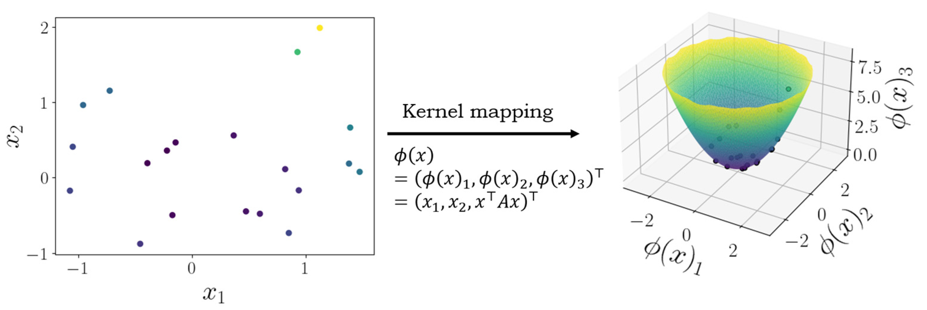
Kernel methods: Kernel methods that are easiest to describe are those that use the so-called kernel trick. Suppose we have access to some n × d data matrix X and an abstract algorithm whose prediction depends on X only through the product XXT>. Here n is the number of training examples, d is the dimensionality of each training input, XT denotes the transpose of X, and XXT is an n × n matrix. If we instead ran our algorithm over some transformation of the data ϕ(X), where ϕ is a function that maps every d-element row of X to a D-element row, the prediction of the algorithm now depends on the matrix ϕ(X)ϕ(XT), which is also an n × n matrix. Under minimal assumptions, given ϕ(X)ϕ(XT), the memory requirements and computational complexity of the algorithm do not depend on D. The data represented in the new space may reveal a structure that was not obvious in the original space. This means that we may lift our original training inputs to a higher dimensional space without incurring additional costs and with potential benefits for the predictor (see Figure 1 for detail). The dimensionality D of the space to which ϕ maps may be very large, or even infinite.
More generally, kernel methods make use of the theory of the reproducing kernel Hilbert space (RKHS), the details of which are beyond the scope of this paper. Briefly, the RKHS can be thought of as very rich function class with elements that cannot always be expressed with a finite number of parameters. Remarkably, the RKHS can be used as a function class in a learning problem for a very large set of losses, and this loss can be minimized with respect to a finite number of parameters using the so-called representer theorem [21].
The process of taking an existing algorithm that operates on XXT and replacing it with a kernel matrix ϕ(X)ϕ(XT) or using the representer theorem is commonly referred to as kernelizing the algorithm. Examples of kernelized algorithms include the support vector machine (SVM) [22], the support vector regression (SVR) machine [23], kernel ridge regression (KRR) [24] and principal component analysis (PCA) [25]. Kernel methods enjoy a rich theory and historical connection with statistical learning theory [26]. As such, mathematically provable generalization guarantees are available for many kernel methods.
Generalized linear models: Generalized linear models (GLMs) [27] are best described as classical statistical methods that generalize ordinary least squares (OLS) regression. In probabilistic terms, OLS assumes that target data Y are samples from a conditionally Gaussian likelihood with a mean that is an unknown parameterized linear transformation of input data X. The parameters of the linear transformation can be computed by solving a linear system, or by running an optimizer such as Newton’s method or gradient descent on the negative log likelihood.
GLMs allow target data Y to be samples from a more general conditional distribution with a canonical parameter that is an unknown linear transformation of input data X. This general conditional distribution is a so-called exponential family. The parameters of the linear transformation are typically found using iteratively reweighted least squares, which is just Newton’s method applied to the negative log likelihood. The negative log likelihood is guaranteed to be convex, and so a properly configured convex optimizer is guaranteed to converge to a global minimum under mild conditions.
GLMs allow one to model situations in which the observed data is not Gaussian. For example, if the data is strictly positive, a Gaussian likelihood is inappropriate, but an exponential likelihood might be appropriate. If the data is integer-valued, a discrete distribution such as the Bernoulli, binomial or Poisson might be used. Just as the Gaussian likelihood corresponds with a squared Euclidean metric, more generally exponential family likelihoods correspond with a certain pasteurization of Bregman divergences [28]. Various machine learning extensions and interpretations of GLMs are available, for example kernelized GLMs [29], although to the best of our knowledge these have not been applied to flood inundation prediction.
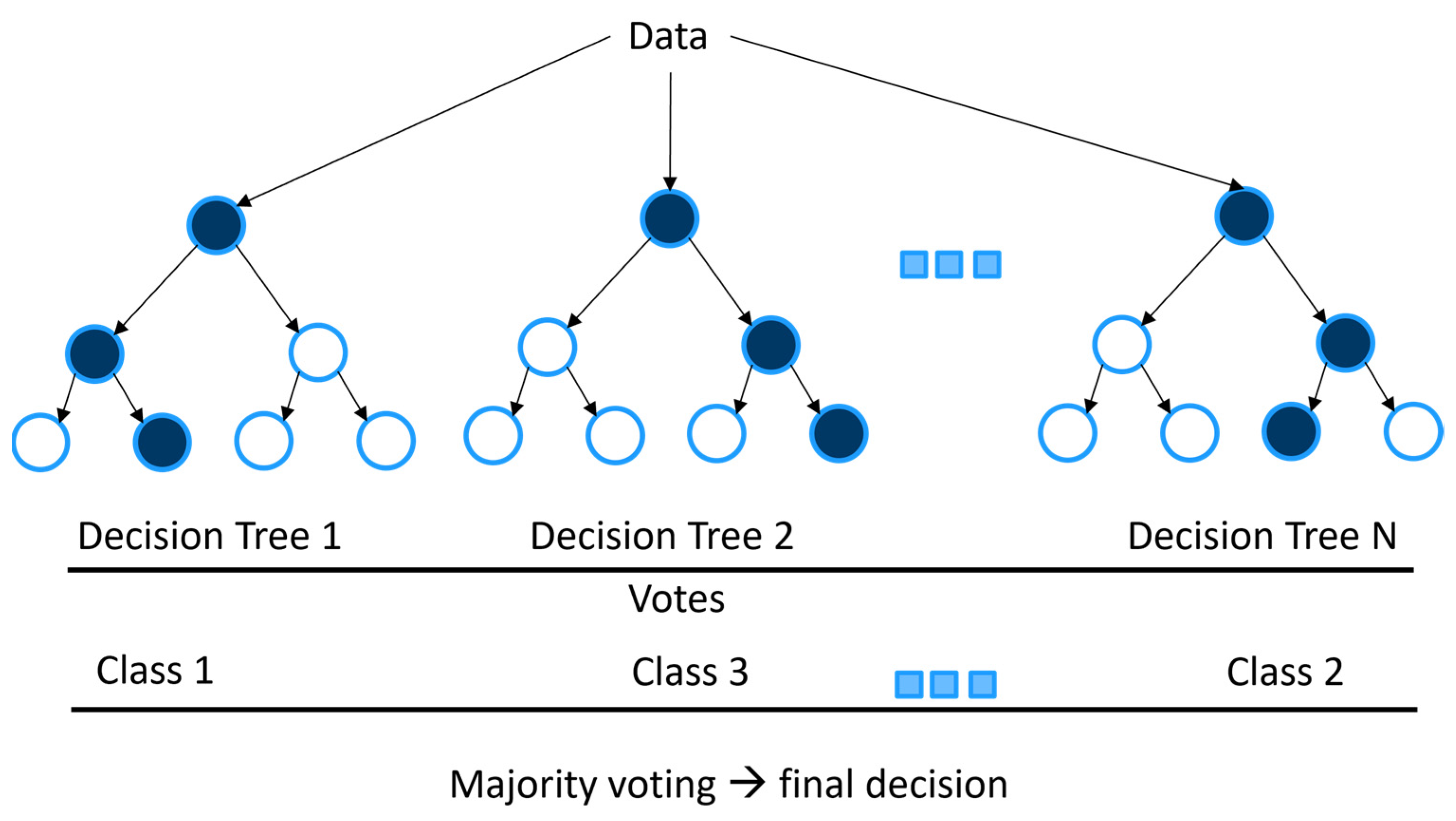
Decision trees, random forest and boosted regression tree: Decision trees [30] are models that use simple decision rules learned from data that can be applied in regression or classification settings. Given a training dataset consisting of inputs and targets, decision trees aim to iteratively partition the input space so that targets with the same or similar values are grouped together. At each iteration, a candidate split is made by selecting some feature and threshold its value. A loss function then measures how desirable the split is, and a split that attempts to minimize this loss is chosen. One example of a loss is the entropy.
Random forest (RF) combines decision trees with bootstrap aggregating (bagging). A random forest is an ensemble of decision trees, each of which is trained on a subset of the training data that is random uniformly sampled with replacement. Other variants of ensembled decision trees include the boosted regression tree. A schematic diagram of RF algorithm is illustrated in Figure 2.
Boosted regression tree (BRT) combines a boosting algorithm with regression tree to increase the performance and reduce the model variance [31].
Other ML related models:
Functional data analysis (FDA): In the example 14 × 5 data matrix in Section 2.2, each row is a data point that is a 5-dimensional vector. Functional data analysis is concerned with data where each data represents a function (hence the name functional). The most common mathematical formulations for dealing with data points are stochastic processes. A stochastic process is capable to represent objects that can be intuitively described as random function. The data points in an FDA technique may represent functions on a regular grid, irregular grid, or even different grids. Due to this advantage, FDA is particularly suitable for dealing with datasets with missing, sparse or irregularly sampled entries.
FDA is a collection of techniques that take this functional view and consists of techniques that generalize methods that work on vector-valued data to function-valued data. For example, FDA techniques for regression, classification, dimensionality reduction and clustering exist. PCA and linear regression are described in Ramsay and Dalzell [32].
Multivariate discriminant analysis (MDA) is a data mining technique which is used to reduce data dimensionality. Using MDA, the multivariate signals are projected down to an N-1 dimensional space. The N represents the number of categories [33].
Multigene genetic programming (MGGP) is known to be a variant of genetic programming [34]. This symbolic optimization method first generates a model (e.g., a tree based model) to map the input to the output data and the updates the model during the training process.
2.2.3. Deep Learning Models
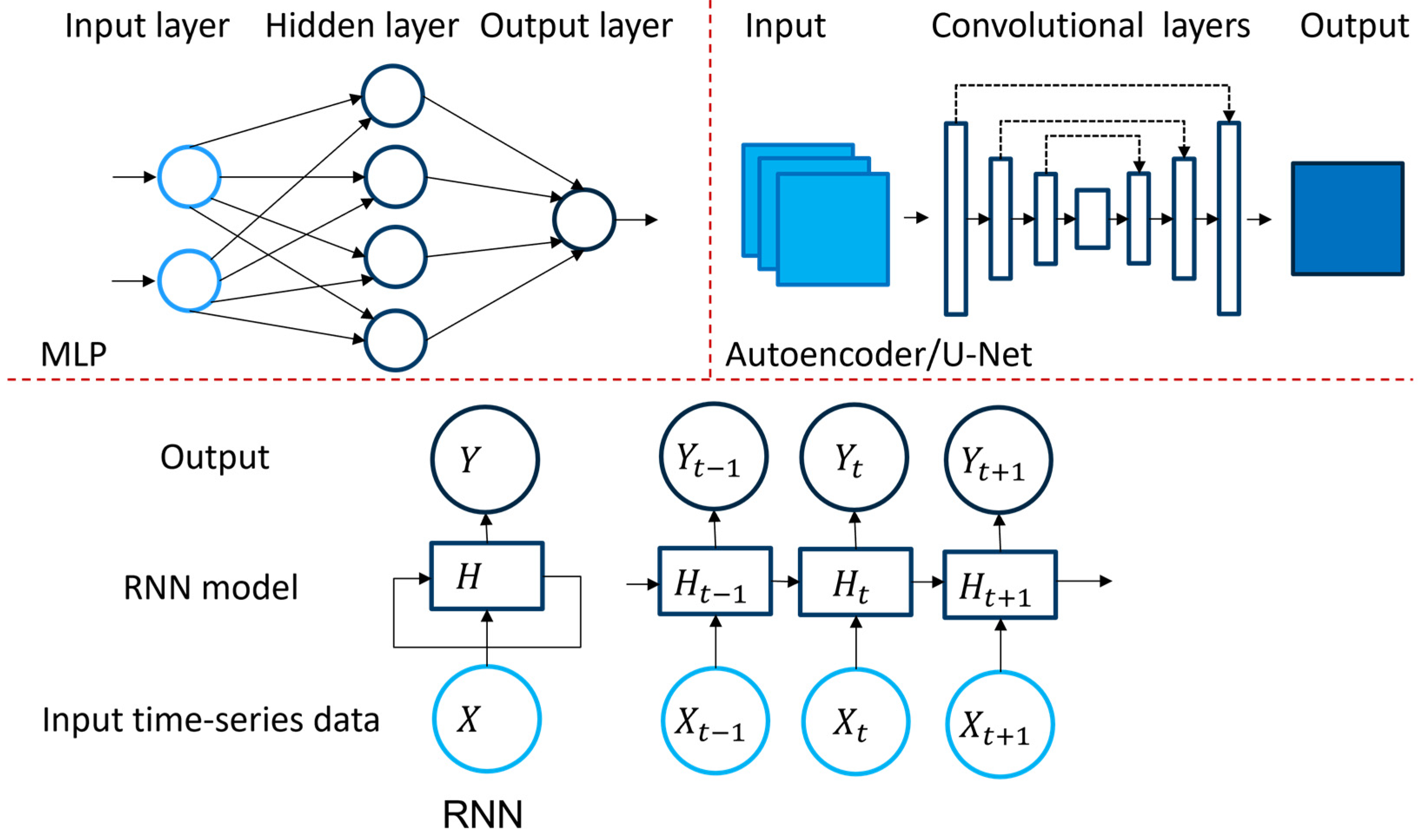
This section summarizes cornerstone neural network architectures used by papers reviewed in this study. Unfortunate historical factors mean that terminology is not always consistent. For example, some use the artificial neural network (ANN) to refer to all deep learning models, whereas some use ANN to refer to a multilayer perceptron (MLP). Our exposition also serves to clarify the terminology employed in our paper. Examples of some of the deep learning models are shown in Figure 3.
Multilayer perceptron: MLPs are flexible function classes that are used as machine learning models. In their most basic form, MLPs compute an output f(x) = z(L) by iteratively applying a sequence of L mappings called fully connected layers,
to an initial input z(0) = x. Here the weights and biases are parameters of the model, and the activation functions are non-linear functions applied coordinate-wise to each vector input. A graphical depiction of an MLP is given in Figure 3.
MLPs can be trained in a similar fashion to GLMs—one typically minimizes a negative log likelihood (or Bregman divergence) or other objective function with respect to the parameters using a numerical solver. In fact, one may show that the mean predicted by a GLM takes the form of a single-layer MLP with the so-called inverse link function as the activation function.
Unlike GLMs, the objective is often non-convex in the parameters when L > 1, and so the numerical solver is unlikely to converge to the global minimum and might not even converge to a local minimum.
The number of parameters in an MLP is typically much larger than a GLM, and so applying second-order or approximate second-order methods can be computationally challenging. Typically, MLPs are applied to datasets larger than would be considered by GLMs, so that the full dataset cannot necessarily be stored in memory and computing the loss (and the first and second derivatives of the loss) is challenging. For these reasons, commonly employed optimization methods for training neural networks are variants of stochastic gradient descent (SGD) [35,36]. There is even evidence to suggest that SGD is important for generalization performance [37]. The most fundamental and famously unresolved theoretical problem in deep learning is understanding why neural networks trained using variants of SGD generalize well in practice [38,39,40,41]; efforts towards understanding progress in this direction are beyond the scope of this paper.
MLPs serve as the most basic neural network prototype. Despite their simplicity, fundamental issues around their large parameter counts, non-convex optimization objectives and generalization performance are inherited by the rest of the deep learning models that follow.
Convolutional neural networks (CNNs): The layer (Equation (1)) is parameterized by unconstrained weights w(l) and biases b(l) which define an affine transformation. One may constrain the weights w(l) to reflect certain locality bias in the input data. This is especially important if the input data is an image, where one expects neighboring pixels to be related. This is the principle behind convolutional layers, which may be viewed as a very large, sparse fully connected layer with repeated entries. Convolutional layers are typically followed by nonlinearities, mirroring the structure in MLPs, and by certain aggregation layers. Aggregation layers include maximum pooling and average pooling.
A CNN or ConvNet comprises at least one convolutional layer. A convolutional layer applies multiple cascaded convolution filters to extract intricate knowledge from the input. Depending on the dimension and nature of input data, convolution kernels can be one, two or three dimensions. Another common layer used within a CNN is a pooling layer. A pooling layer is used to reduce the size of the input while keeping the positional knowledge intact. A frequently used pooling method within CNN literature is Maximum Pooling.
Autoencoders: Autoencoders consist of two networks, the encoder and decoder, in series. The encoder maps the input to another space (typically of lower dimension) called the embedding space, and the decoder attempts to map from the embedding space back to the input. The parameters of the encoder and decoder are jointly learned by minimizing and objective that says that the input of the encoder should in some sense be close to the output of the decoder. The encoder and decoder may consist of any layers, for example fully connected or convolutional layers. The output of the decoder is called the bottleneck layer, named as such for the shape as shown in Figure 3.
U-Net: A U-Net is a variant of an autoencoder that includes skip connections. It was originally designed for biomedical image segmentation [42] with a particular architecture (number of layers, sequence of layers, dimensions of layers, type of activation function, etc.) but now refers to a more general U-Net type structure.
Generative adversarial network (GAN) is a generative model, aiming to generate samples from a distribution given only a finite number of samples from that distribution [43]. GANs consist of two networks, a generator and a discriminator. The generator aims to generate artificial samples from the target distribution, and the discriminator aims to distinguish between real samples and artificial samples. The parameters of the generator and discriminator are jointly optimized according to this objective.
Recurrent neural networks (RNNs) models introduce the notion of time into a deep learning model by including recurrent edges that span adjacent time steps [44]. RNNs are termed recurrent as they perform the same task for every element of a sequence, with the output being dependent on the previous computations. Long short-term memory (LSTM) type DL models were proposed to provide more flexibility to RNNs by employing an external memory, termed the cell state to deal with the vanishing gradient problem [45]. Three logic gates are also introduced to adjust this external memory and internal memory. Gated Recurrent Unit (GRU) is a variant of LSTMs which combine the forget and input gates making the model simpler [46].
3. Application of Machine Learning for Flood Inundation Modeling
3.1. Traditional Machine Learning Approaches
We organize our discussion on traditional machine learning approaches in terms of the task (classification, regression) that they solve. Each task can be solved using a number of models, which we described in Section 2.2. A summary of these works is presented in Table 2.
3.1.1. Classification
El-Haddad et al. [47] investigated four data mining/machine learning models to predict flood susceptibility maps in Wadi Qena Basin in Egypt. They set up a classification problem that classifies regions in a fine grid as having or not having a flood occur at a particular time points. The model accepts input data X containing flood influencing variables over a geographical region including slope angles, land-use data, lithological data, a topographic wetness index, altitude, slope length, shape, and aspect. The model returns binary outputs that are made to agree with response data Y, indicating whether a flood occurred or not. The data to train the models was obtained from 342 inundation locations and included of three flood influencing factors (distance from main channel, land use/cover and lithological units).
Four classification models were employed for these tasks: boosted regression tree (BRT), logistic regression (a type of GLM), a pipeline of functional data analysis techniques (FDA), and multivariate discriminant analysis (MDA). It is not clear which instance of GLM is used; the authors mention that logistic regression (corresponding with Bernoulli targets) and linear regression (corresponding with Gaussian targets) are used, but only provides results for a model referred to as GLM. The reported results are that BRT, FDA, GLM, and MDA models can generate a flood susceptibility mapping with a reasonable accuracy.
Avand et al. [48] investigated the effects of digital elevation model (DEM) spatial resolution on ML classification models including RF, MLP and GLM. In this study 220 flood locations from Yasouj-Dena watershed (Iran) were chosen along with 14 causative factors in the flood as independent variables. The data generated from two flood models were of size 12.5 and 30 m. They divided the Flood Probability Map (FPM) into five classes as very low, low, moderate, high, and very high. Their results indicated that using 12.5 m spatial resolution data to predict flood map is more consistent and accurate with the flood points in the study area in comparison to 30 m spatial resolution data.
Madhuri et al. [49] applied five ML classification models, namely (i) Logistic Regression, (ii) Support Vector Machine, (iii) K-nearest neighbor (KNN), (iv) Adaptive Boosting (AdaBoost) and (v) Extreme Gradient Boosting (XGBoost) to classify locations into flooded or no flooded regions. They used 10-fold cross validation method to train and validate these ML methods. Among the applied ML models, XGBoost demonstrated the best performance for both flood prediction and flood susceptibility mapping.
Talukdar et al. [50] utilized six machine learning techniques including ANN, SVM, RF, Maximum likelihood, Parallelepiped, Spectral Information Divergence to map the wetland inundation and investigated the changes in inundated area through wetland fragmentation analysis. In this work, the area of wetland predicted by each classifier is different, the maximum and minimum wetland areas generated by ANN and SVM classifier respectively. Regarding the validation of ML model on this data, SVM demonstrated the highest accuracy and parallelepiped showed the least. One of the challenges related to this study is the lack of high-resolution data for wetlands to model the flood.
Ma et al. [51] introduced the XGBoost model to assess the flash flood risk and applied this model to predict flash flood risk in data obtained from Yunnan Province, China. They compared their proposed model with the least squares support vector machine (LSSVM), which indicated the high performance and effectiveness of XGBoost. Their results also showed that the accuracy of the model depends on the amount of flash floods fall into a region. For the low-risk areas flash flood did not impact the results of LSSVM and XGBoost, whereas for medium-risk area LSSVM worked better and for high and highest-risk areas XGBoost demonstrated higher accuracy.
Karimi et al. [52] predicted the daily wetland inundation pattern of a segment of the Darling River in Australia using RF. Their study showed that topography and discharge are the most influential variables in predicting inundation occurrence. While due to computing efficiency the ML model approach was a reasonable option to model long-term daily inundation, yet this model suffered from lack of generalization to new data.

Table 2.
Summary of traditional ML approaches for inundation analysis.
| Authors | Publication Year | Application | Approach |
|---|---|---|---|
| Avand et al. [48] | 2022 | Effects of DEM resolution | RF, MLP, and GLM |
| Yan et al. [53] | 2021 | Estimating flow depth | MGGP |
| El-Hedad et al. [47] | 2021 | Flood risk assessment | BRT, FDA, GLM, MDA |
| Madhuri et al. [49] | 2021 | Flood risk assessment | Logistic Regression, SVM, KNN |
| Ma et al. [51] | 2021 | Flood risk assessment | XGBoost, LSSVM |
| Hou et al. [54] | 2021 | Urban flooding | RF, KNN |
| Yuan et al. [55] | 2021 | Road flooding | RF, AdaBoost |
| Talukdar et al. [50] | 2021 | Wetland inundation | RF, SVM, MLP |
| Karimi et al. [52] | 2019 | Wetland inundation | RF |
3.1.2. Regression
Hou et al. [54] developed a hydrodynamic based urban flood model to generate data to train ML models for urban flood prediction. They used k-nearest neighbor algorithm (KNN) and RF as their ML models and showed combination of these models could perform better than using them separately to predict inundation area, depth and volume. The final forecast results for the test study area could be obtained by merging the results inferred from hydrodynamic numerical model and ML results.
Yan et al. [53] leveraged the MGGP as an optimization method to model the spatial distribution of flow depth in fluvial systems. They employed their model on data generated from a section of the Ottawa River and divided the region into sub-regions. The MGGP model was separately trained for each sub-region which resulted in 500 models. Although this approach reduced the complexity, sub-regions (meshes) have no inner connection during training, which can reduce the final performance.
3.2. Deep Learning Approaches
Due to their high performance and capability to represent complicated functions to map data from one domain to another, deep learning models have been widely used in different fields. In recent years, deep learning has received more attention within the flood modeling community to model flood inundation and predict water depth and extent. In this section, we review papers which modeled the flood inundation through deep learning; a summary of these works is presented in Table 3.
3.2.1. Multilayer Perceptron (MLP)
Berkhahn et al. [56] developed an MLP to predict the water levels during flash flood events. The input to the MLP is rain events at different time steps and the output is the maximum water level. They tested their model on synthetic rain event data obtained from two modified urban catchments. The results inferred from the MLP model were compared with those from the physical model. They demonstrated the capability of MLP in predicting water levels for pluvial floods in real-time.
Tamiru and Wagari [57] integrated machine learning with HEC-RAS (a software for modeling river flow [58]) as hydraulic model to estimate runoff and the extent of flood in Baro River Basin, Ethiopia. They first trained an MLP using spatiotemporal data including daily rainfall and temperature data of the same period (1999–2005) and the Topographical Wetness Index to predict runoff. The output of the ANN model then passed to HEC-RAS software to generate the flood extent along the river. The outcomes of this research study denoted that integration of ANN and HEC-RAS to generate stream flow and water depth respectively could produce high quality water inundation which can be used for risk management system.
Hosseiny et al. [59] developed a hybrid model for flood inundation. Their pipeline consists of a two-dimensional hydraulic model, iRIC (International River Interface Cooperative) and ML model. The ML model has two parts; (i) random forest (RF) to identify wet or dry nodes over the domain, (ii) MLP model to estimate river depth in wet nodes. Using this pipeline, they achieved a high accuracy in classifying wet and dry area and predict the water depth.
Chu et al. [60] modeled the flood inundation and investigated the application of ANN for the flood inundation model. The ANN-based emulation modeling framework consists of the generalized regression neural network (GRNN) which is feed forward network and does not require an iterative training. They showed that GRNN is able predict flood extend with high accuracy in a shorter time in comparison to physical model. Zhu et al. [61] deployed an MLP model similar to Chu et al. [60]. Their model takes the hydrographs of the rivers that contribute to the flooding in the urban area as inputs, and the outputs are the water depths at each pixel in all grids. They trained MLP models for their case study area and investigated several optimization algorithms. The comparison of results showed superiority of the MLP models that were trained on hybrid dataset (synthetic + real) over synthetic dataset.
3.2.2. Convolutional Neural Networks
One dimensional CNN: Kabir et al. [62] investigated the application of CNN model to predict inundation from flash flooding and compared it with support vector regression (SVR) as a traditional ML model. Their model consists of two 1D-convolutional layers and three MLPs. The inputs to the model are the upstream flow discharge values at different time steps and the outputs is an array of water depth based on the number of cells in the simulation domain. The objective function to train the CNN model is the mean square error (MSE). The water depth predicted by the CNN for the real events then converted to spatially distributed flood maps and compared with the output of traditional DEM.
Their results indicate that their one-dimensional CNN model can predict the water depth throughout the whole flood event with a reasonable accuracy and can outperform the SVR models. The accuracy of SVR models can be increased by increasing the number of samples which results in an increase in the number of SVR models and thus the computational time. Further, one CNN model is sufficient to learn to predict the water depth from inflows, whereas the number of SVR models is dependent on the number of locations. For instance, in this study 18 SVR models are separately trained to predict water depth at 18 different locations while only one CNN model is trained to perform the same task.
Segmentation-based approaches: Hosseiny [63] studied a segment of the Green River, 120 km downstream of the Flaming Gorge Dam in the northeast corner of Utah, USA. They modified the U-Net [42] to predict water depth and extent. The main reasons to choose this model were the capability of U-Net to learn from relatively small amount of data and their geometry. The input to their U-Netriver was a composite image with two bands including the ground elevation and flooding discharge of size 128 × 128 pixel, and the output was water depth. The objective function to train the network was MSE. The application of the U-Netriver for different discharges demonstrated its capability of detecting the river geometry including the river width, shape, curves, and even the river splits around the island. In comparison to traditional ML model [59] applied on the same data, their model not only demonstrated a reduction of 29% in the reported error, but also eliminated the requirement of a separate classifier to classify grids to the wet or dry regions. One of the main weaknesses of this model is its generalizability. While the trained model showed high performances for the lower depth values (lower discharges), it requires an improvement to deal with high discharges or out of training discharge data.
Löwe et al. [64] also developed a U-Net based model called U-Flood to predict the urban pluvial flood water depth. They investigated 11 spatial variables that could be generated from geographic data as direct inputs to U-Flood and fused the rainfall data obtained from gauges observation to the middle layer of the U-Flood to predict flood depth.
They investigated two approaches to find the optimal number of spatial variables as input data to the U-Flood model as Spearman correlation [65] and forward selection. Their results denoted that combination of five spatial data (e.g., flow direction, water depth, velocity and terrain curvature) as input could yield the best performance. Further, they applied PCA to reduce the number of inputs from 11 to 7 and inferred comparable results.
They also investigated the hyper-parameters and structure of the proposed U-Flood. Their results showed that a U-Flood with 28 million trainable parameters could be an optimal network. One of the challenges in this paper was the demands for considering the number temporal raining events due to the computational limitation by CNN.
3.2.3. Autoencoder Approaches
Guo et al. [66] investigated the application of autoencoders as a deep learning model on data obtain from three catchments named Luzern, Zurich, Switzerland, and Coimbra, Portugal. Unlike Hosseiny [63] and Löwe et al. [64] their proposed model does not include skip connections. Their CNN model accepts two types of data as input; (i) terrain patches which represent the surface features of size 256 × 256 × 5 (height, width and five channels), (ii) rainfall hyetographs as one-dimensional vector which represents the average rainfall intensity in a 5-min interval. The output of the network is the prediction of the water depth. One of the challenges within flooding data is the variation of water depth in different areas (shallow/deep water) which results in imbalance data, this has been addressed by using a weighted mean square error as the objective function to learn the water depth from input data. The results of test data were reported using the mean absolute error (MAE). The validation results indicate that Autoencoders can be a reliable fit to predict water depth (shallow and deep) for pluvial events. In this study, both spatial (elevation) and vectors (hyetographs) were used as input to the DL model and the results demonstrated high accuracy and the ability of the DL model to be generalized to real rain fall events.
3.2.4. Adversarial Approaches
Hofman et al. [67] proposed a generative adversarial network (FloodGAN) to predict pluvial flooding caused by nonlinear spatial heterogeny rainfall events. Their method consists of three stages as follow: (i) generate synthetic data from rainfall events, (ii) train the FloodGAN model to learn the relationship between rainfall distribution and corresponding water depth by which it can predict the depth, and (iii) online prediction of water elevation from rainfall events.
Results showed similar root mean square error (RMSE) for water depth estimation when compared to other simulation-based screening approaches [68]. While the proposed model could predict the water depth in depression area well, prediction of shallow flooding on surface flow paths outside depressions remains a challenge.
FloodGAN directly infers the flood hazard maps from raw rainfall images, this image-to-image translation approach allows end to end training paradigm for flood prediction with a reasonable accuracy. In addition, the FloodGAN was tested on both synthetic and real rainfall dataset and demonstrated generalizability of the proposed model along with a dramatic computational enhancement (106 times faster than 2D hydraulic models). However, FloodGAN trained using only synthetic data and the results compared to a hydraulic model rather than any other deep learning algorithm. In addition, they only focused on predicting maximum inundation extent and water depth for up to 1-h rainfall events and did not include the prediction of flow velocities. Another drawback of the proposed model is that it does not take the serial correlation of time series data of flooding into account and the prediction results are limited to quasi-static flood hazard maps.
3.2.5. Spatio-Temporal Analysis Approaches
Recent studies investigated the adoption of deep learning approaches for flood related tasks. Zhou et al. [19] modeled time series and reduced information redundancy in flood inundation data using long-short-term memory networks and a spatial reduction model. They developed 500 LSTM to model flood for 125 representative locations, and their experimental results showed only 125 LSTM were enough to reconstruct the flood inundation surface.
Wei [69] predicted the water levels in catchment areas during typhoons through sequential neural networks (SNNs), multiple input functional neural networks (MIFNNs) and conventional regression-based (REG) model. The SSN model consists of dense LSTM layers and take 1-D data (e.g., water levels at river station, rainfall intensity, and reservoir release of Feitsui Reservoir) as input, whereas the MIFNNs model is designed to take 2-D data (e.g., radar reflectivity mosaics obtained from the central weather bureau) as input and passing them to convolutional layers and then concatenate the feature extracted from CNN with 1-D data and pass them to LSMT layers to predict the water level. In their study they investigated 16 typhoons which caused major rainfall in the Hsintien River (Taiwan). The drainage area of the studied region is approximately 916 km2 with a total length of 84.6 km.
The results from Wei [69] indicated that MIFNN model had the best performance in comparison to SNN and REG model. This means that using multi modal data such as radar reflectivity images and water levels at river stations along with a MIFNN like model could enhance the performance of water level prediction.
Tsakiri et al. [70] developed a hybrid model for forecasting river flood events. This hybrid model consisted of multiple linear regression models (MLR) or the MLP model and time series decomposition to predict the water discharge. Their results proved that before the application of any model it is necessary to decompose the time series for water discharge into long-, seasonal-, and short-term components. The comparison of MLP and MLR showed superiority of MLP in forecasting the water discharge.
Table 3.
Summary of DL approaches for flood inundation modeling.
| Authors | Publication Year | Application | Approach |
|---|---|---|---|
| Guo et al. [66] | 2021 | Urban flood emulation | Autoencoder |
| Löwe et al. [64] | 2021 | Urban flood depth (pluvial) | U-Net |
| Hosseiny [63] | 2021 | Flood depth | U-Net |
| Hosseiny et al. [59] | 2020 | Flood depth | MLP & RF |
| Wei [69] | 2020 | Flood depth | LSTM |
| Zhou et al. [19] | 2021 | Flood inundation | LSTM |
| Zhu et al. [61] | 2021 | Flood Inundation | MLP |
| Hofman et al. [67] | 2021 | Flood inundation (pluvial) | GAN |
| Tamiru and Wagari [57] | 2021 | Flood inundation | MLP & HEC-RAS [58] |
| Chu et al. [60] | 2020 | Flood inundation | GRNN |
| Kabir et al. [62] | 2020 | Flood inundation (fluvial) | 1-D CNN & SVR |
| Tsakiri et al. [70] | 2018 | Flood inundation | Linear regression, MLP |
| Berkhahn et al. [56] | 2019 | Flood inundation (pluvial) | MLP |
3.3. Datasets
One of the main components of ML approaches is a well curated dataset. This section briefly describes the datasets that are used in previous studies to train and validate DL or ML algorithms.
Yan et al. [53] investigated the fluvial flood event in a segment of the Ottawa River, Canada covering an area of 3.2 × 1.40 km2. They used TELEMAC-MASCARET hydrodynamic model [71] simulated water level data to train their MGGP model. They divided the study region into 34 sub-regions and provided around 10,000 data points for each sub-region.
El-Haddad et al. [47] study covered an area of 14.5 km2 in the Wadi Qena Basin in Egypt. The data were derived from 342 inundation locations by analyzing satellite imagery and geological and topographical maps. They used 30 × 30 m pixel flood data and considered three flood influencing factors (e.g., distance from main channel, land cover and soil type) for training their data mining/machine learning models About 70% of the data were used for training the model and the remaining 30% data were used for validating.
Avand et al. [48] studied 220 flood locations from Yasouj-Dena watershed in Iran. They investigated 14 causative factors of floods as independent variables and assessed the impacts of spatial resolution on ML classification models. They used DEMs of size 12.5 and 30 m spatial resolution derived from ALOS PALSAR [72] and Advanced Space-borne Thermal Emission and Reflection Radiometer (ASTER) [73] respectively. They divided the flood probability map (FPM) into five classes as very low, low, moderate, high, and very high and evaluated predicted flooded area with measured flood data.
Madhuri et al. [49] used data from 295 flood locations in Greater Hyderabad Municipal Corporation in India. Their study covered an area of 625 km2 and it was divided into 16 zones. They used a geo-spatial database based on ASTER DEM (30 × 30 m spatial resolution) using eight flood factors [74,75]. Their ML models were evaluated against historical flood data of 2000, 2006 and 2016.
Hou et al. [54] investigated multiple ML models for urban flood forecasting in the Shaanxi Province, China. They validated their model for the part of Fengxi New Town covering an area of 2.43 km2. They used hydrodynamic model simulated inundation data and rainfall characteristic parameters to train ML models. Data from 150 rainfall events were used for training and 30 events for validating ML models.
Talukdar et al. [50] studied a wetland of size 3669.58 km2 in the Sunamganj district of Bangladesh. They used 30 m resolution satellite data acquired from the Landsat imagery. They reported that lack of high-resolution data for wetlands was a major challenge for validating ML models for wetland inundation.
Ma et al. [51] investigated flash flood in the Yunnan Province in China using XGBoost ensembles method. They used measured and satellite-based flash flood data for the period of 2011 to 2015 for training the ML models. Another set of flood data from 2018–2019 were used for verifying the accuracy of risk maps derived from ML model.
Karimi et al. [52] studied inundation pattern of a segment of the 1200 km2 of Darling River in Australia (1200 km2) using RF machine learning technique. They used a set of dependent variables (e.g., inundation area) and another set of independent variables (e.g., topographic, climatic), describing hydrological and physical characteristics of the study area to configure and validate the ML models. The dependent variables were 30 m resolution gridded inundation map obtained from Landsat imagery. From the raster data 10,000 points were randomly selected for the ML model.
Tsakiri et al. [70] studied the Mohawk River basin in the USA with length of 240 km. They used precipitation time series, daily water discharge, temperature, groundwater level, wind, speed and tide data to develop their DL models. They derived the water discharge and groundwater data from the United States Geological Survey (USGS) gage stations from 2005 to 2013. To explain the water discharge time series, they used Decomposition–Kolmogorov–Zurbenko. The atmospheric data were obtained from the National Oceanic and Atmospheric Administration (NOAA) database.
Zhu et al. [61] dataset included 360 flood events: 180 were synthetic flood events generated by FloodEvac tool, and 180 were additional real flood events from three major rivers in Kulmbach, Germany in the period of 1970 to 2017. The area of the study was divided into a 50 by 50 mesh covering 2500 grids.
Berkhahn et al. [56] generated flood data for validating their ANN models using a physically based coupled surface and sewer network model, commonly known as Hystem-Extran 2D [76]. They tested the ANN models for 3 grid sizes of 3, 6 and 9 m and applied the models for 2 case studies, one with flat land and the other with steep slope.
Tamiru and Wagari [57] generated inundation data from an area of 74,100 km2 in Baro River Basin (Ethiopia). The data was collected and generated for seven years from 1999 to 2005. They also curated test data for three years from 2006 to 2008.
Chu et al. [60] studied a part of the Burnett River in Central Queensland, Australia. The river system has a total catchment area of more than 33,000 km2 and the area of the study is 2720 m × 2860 m. This area is represented by 19,448 grid cells of size 20 m by 20 m by using the TUFLOW hydrodynamic model [77]. Their DL models were tested for 10 flood events including three historical events (i.e., year 1971, 2010 and 2013) and seven “design events”.
Zhou et al. [19] studied flood inundation in the Burnett River system downstream of Paradise Dam in Queensland, Australia. The data for this area was generated by developing a 2D hydraulic model using TUFLOW [77]. This model contains 3,697,597 grid cells of size 20 m by 20 m and covers almost 1479 km2 area.
Wei [69] used gauged rainfall and water level data from 3 river stations for 16 typhoons in the Hsintien River in Taiwan. They also used hourly reflectivity data from 2952 radar mosaics for spatial rainfall data to train and validate their SNN and MIFNN models. The drainage area of the studied region is approximately 916 km2 with a 84.6 km river reach.
Hofman et al. [67] studied an area of 2 km by 2 km of the city center of Aachen, Germany. They generated 901 synthetic rainfall events and grouped them into eight classes of 5 mm/hour steps. They simulated water levels corresponding to each rainfall event using the MIKE 21 hydrodynamic model [78].
Guo et al. [66] used simulated data in their study which is generated from two DEM software; (i) CADDIES cellular-automata flood model [79], and Infoworks ICM software [80]. In general, 18 one-hour rainfall events were created based on return periods for the simulations. The grid size of the simulated data for the raster is 1 m with minimum time step of 0.01 s. A total of 10,000 patch locations were randomly sampled for each catchment area and the data were split into train and test data.
Löwe et al. [64] used MIKE21 hydrodynamic model [78] to generate flood maps from 53 rain events (available in this study), the size of each patch was 256 m by 256 m pixels. In addition, rainfall data including the rainfall intensity collected from observed data of 1 min resolution from 10 rain gauges distributed across Denmark was processed and resulted in 53 events.
Hosseiny [63] used a two-dimensional hydraulic model (iRIC, [81]) to generate flood discharge and depth data. They used 8.3 × 8.3 m gridded elevation and discharge data for training their DL model (U-Netriver) and depth data for validating their U-Netriver model. They investigated an area of 260 × 251 pixel (4.5 km2) of which 128 × 128 pixels were randomly selected for training the model.
The study of Kabir et al. [62] covered an area of 14.5 km2 of the urbanized area of Carlisle city in England. They generated flood depth data for training the CNN deep learning model from eight synthetic hydrographs using LISFLOOD-FP hydrodynamic [82]. They divided the study area into 581,061 grids and used water depth as the controlling parameter for validating the CNN model. In addition to synthetic depth data for training, two sets of measured data for 2005 and 2015 floods were used to validate the CNN model.
A summary of all datasets is presented in Table 4. It demonstrates a wide variability in the source of data and models that were used to generate input data. All studies emphasized the importance of large data sets for training and validating ML models. The majority of these studies used hydrodynamic model-generated flood data for training ML/DL algorithms because measured and/or remotely sensed flood inundation data were insufficient for training/validating such models. Lack of publicly available benchmark data limits the rigorous testing of ML and DL technologies in the field of flood inundation. These challenges are also mentioned in other studies (e.g., Sit et al. [2]).
4. Strength and Limitations of ML/DL Models
4.1. Strength
ML models and recently advanced DL models demonstrated outstanding performance in modeling flood inundation with high accuracy. Using ML/DL sequential events (e.g., water level in a period [69]), time independent events (e.g water depth based on discharge [63] or wet or dry land prediction [59]).
The application of ML and specifically DL algorithms on flood events have shown the remarkable ability of these models to learn to predict flood inundation. The key challenges that are partially addressed by ML/DL models are reducing the computational time for simulating flood forecasting to real/near real-time. For instance, a case study by Chu et al. [60] showed that simulating a flood event using TUFLOW model takes over 200 h whereas a DL model can achieve this in 1 min.
4.2. Limitations and Open Research Challenges
4.2.1. Generalizability
One of the major limitations of ML/DL models in a real-world scenario is the generalizability of these models. In other words, these models have difficulty in predicting something beyond the data used to train them [60]. This is even more challenging when these models are trained with synthetic data and tested on real scenarios or when the models are trained on data obtained from small regions. An example of the comparison of the efficiency of ML models using different types of data is presented in [61].
While both ML and DL models showed high ability in modeling flood events, more advanced DL models such as U-Netriver [63] and FloodGAN [67] demonstrated better performance. Advanced DL models can cover greater regions for training whereas the ML or basic DL models (e.g., MLP) require to be trained on small grids, this also increases the number of ML models to model flood in a region [61].
4.2.2. Dataset
Our review on flood events datasets revealed the lack of a publicly available bench- mark dataset to compare the performance of ML/DL flood inundation models. In other fields such as computer vision, it is common to publish datasets and researchers will investigate their DL models using these datasets (e.g., COCO dataset [83]). This challenge is also mentioned in other flood study reviews (e.g., Sit et al. [2]). Flood events data are obtained from different resources, and geopolitical limitation can make the situation even more difficult to publish a generic dataset. We recommend publishing generic data that includes all flood inundation related parameters from a less sensitive geopolitical region or synthetic data which are close to real situations. Such a dataset can help to build more stable and generalizable DL methods for flood forecasting.
4.2.3. Embedding Expert Knowledge
ML algorithms are designed to learn a mapping function from input to output data. In flood inundation, input data are obtained from several resources and always require manual calibration by experts. In inundation, calibration refers to a trial-and-error process to estimate model parameters. As in other research fields, such as biology, precious domain knowledge can be used for training ML/DL models to improve the performance of such models.
4.2.4. Application of Graph Neural Network and Neural Operators
In flood modeling, usually modelling domains are divided into raster grids with a specific resolution. These grid-based data are then used to train ML/DL models to predict water depth, flooding extent, and volume of water.. Most of the current ML/DL models that use grid-based data to learn mapping functions, suffer from understanding the interaction between grids whereas this is not an issue in hydraulic modelling. Graph neural networks (GNNs) are one of the powerful ML tools that can be applied on flood events, GNNs can interpret each gird as a node and connect them through graph construction.
4.2.5. Explainability
Machine learning models are known as black box. These models take input data from other sources and predict the output. Providing information of why and how a certain prediction has been made, a ML/DL model can help not only to boost the performance of these models but also increase the trustability of such models. For instance, when more than one input (atmospheric + geographic) is used to train a model to predict water depth, how this extra information can participate in producing the results can be investigated by explainability.
5. Conclusions
In this paper, we reviewed and compared ML and DL methods to model flood inundation in different river basins. The applications of traditional ML and DL methods for flood modeling have shown the remarkable ability to predict flood inundation for different hydrological and landscape conditions. The ML/DL models are found particularly advantageous for real-time flood simulation which is a key challenge for physically based models because of longer simulation time. One of the major limitations of ML/DL models is generalizability. This is even more challenging when these models are trained with synthetic data. While both ML and DL models showed high ability for flood inundation modeling, more advanced DL models such as U-Netriver and FloodGAN demonstrated better performance. Apart from strengths and weaknesses of such methods, challenges and future research avenues related to application of ML/DL models to model inundation events have been discussed.
Author Contributions
Conceptualization, F.K., M.A.A., D.A.-A., L.T.-S. and L.P.; methodology, F.K., M.A.A. and D.A.-A.; formal analysis, F.K., M.A.A. and D.A.-A.; investigation, F.K., M.A.A. and D.A.-A.; resources, F.K., M.A.A. and D.A.-A.; data curation, M.A.A., D.A.-A. and L.T.-S.; writing—original draft preparation, F.K. and M.A.A.; writing—review and editing, F.K., M.A.A., D.A.-A., L.T.-S. and L.P.; visualization, M.A.A., D.A.-A. and L.T.-S.; supervision, F.K. and L.P.; project administration, F.K. All authors have read and agreed to the published version of the manuscript.
Funding
This research was funded by the Commonwealth Scientific and Industrial Research Organisation through its Digital Water and Landscape (DWL) project.
Data Availability Statement
Data will be available on request.
Acknowledgments
We thankfully acknowledge valuable input from Russell Tsuchida of CSIRO in an earlier version of this manuscript.
Conflicts of Interest
The authors declare they have no known competing financial interests or personal interest that could have influenced the work reported in this paper.
Nomenclatures
| AdaBoost | Adaptive Boosting |
| ANN | Artificial neural network |
| ASTER | Advanced Space-borne Thermal Emission and Reflection Radiometer |
| BRT | Boosted regression tree |
| CNN | Convolutional neural network |
| DL | Deep learning |
| FDA | Functional data analysis |
| FPM | Flood probability map |
| GAN | Generative adversarial network |
| GLM | Generalized linear models |
| GPU | Graphics processing unit |
| GRNN | Generalized regression neural network |
| GRU | Gated recurrent unit |
| HD | Hydrodynamic |
| HEC-RAS | Hydrological Engineering Center—River Analysis System |
| iRIC | International River Interface Cooperative |
| KNN | k-nearest neighbour algorithm |
| KRR | Kernel ridge regression |
| LSSVM | Least squares support vector machine |
| LSTM | Long short-term memory |
| MAE | Mean absolute error |
| MDA | Multivariate discriminant analysis |
| MGGP | Multigene genetic programming |
| MIFNN | Multiple input functional neural network |
| ML | Machine learning |
| MLP | Multilayer perceptron |
| MLR | Multiple linear regression |
| MSE | Mean square error |
| NOAA | National Oceanic and Atmospheric Administration |
| OLS | Ordinary least squares |
| PCA | Principal component analysis |
| REG | Conventional regression |
| RF | Random Forest |
| RKHS | Reproducing Kernel Hilbert Space |
| RMSE | Root mean square error |
| RNN | Recurrent neural network |
| SGD | Stochastic gradient descent |
| SNN | Sequential neural network |
| SVM | Support vector machine |
| SVR | Support vector regression |
| USGS | United States Geological Survey |
| XGBoost | Extreme gradient boosting |
References
- Bentivoglio, R.; Isufi, E.; Jonkman, S.N.; Taormina, R. Deep Learning Methods for Flood Mapping: A Review of Existing Applications and Future Research Directions. Hydrol. Earth Syst. Sci. Discuss. 2022, 26, 4345–4378. [Google Scholar] [CrossRef]
- Sit, M.; Demiray, B.Z.; Xiang, Z.; Ewing, G.J.; Sermet, Y.; Demir, I. A comprehensive review of deep learning applications in hydrology and water resources. Water Sci. Technol. 2020, 82, 2635–2670. [Google Scholar] [CrossRef]
- Mudashiru, R.B.; Sabtu, N.; Abustan, I.; Waheed, B. Flood Hazard Mapping Methods: A Review. J. Hydrol. 2021, 603, 126846. [Google Scholar] [CrossRef]
- Ghorpade, P.; Gadge, A.; Lende, A.; Chordiya, H.; Gosavi, G.; Mishra, A.; Hooli, B.; Ingle, Y.S.; Shaikh, N. Flood Forecasting Using Machine Learning: A Review. In Proceedings of the 2021 8th International Conference on Smart Computing and Communications (ICSCC), Kochi, India, 1–3 July 2021; pp. 32–36. [Google Scholar]
- Mosavi, A.; Ozturk, P.; Chau, K.w. Flood prediction using machine learning models: Literature review. Water 2018, 10, 1536. [Google Scholar] [CrossRef]
- Teng, J.; Jakeman, A.J.; Vaze, J.; Croke, B.F.; Dutta, D.; Kim, S. Flood inundation modelling: A review of methods, recent advances and uncertainty analysis. Environ. Model. Softw. 2017, 90, 201–216. [Google Scholar] [CrossRef]
- Bulti, D.T.; Abebe, B.G. A review of flood modeling methods for urban pluvial flood application. Model. Earth Syst. Environ. 2020, 6, 1293–1302. [Google Scholar] [CrossRef]
- Liu, Q.; Qin, Y.; Zhang, Y.; Li, Z. A coupled 1D–2D hydrodynamic model for flood simulation in flood detention basin. Nat. Hazards 2015, 75, 1303–1325. [Google Scholar] [CrossRef]
- Horritt, M.; Bates, P. Evaluation of 1D and 2D numerical models for predicting river flood inundation. J. Hydrol. 2002, 268, 87–99. [Google Scholar] [CrossRef]
- Leandro, J.; Chen, A.S.; Djordjevic, S.; Savic, D.A. Comparison of 1D/1D and 1D/2D coupled (sewer/surface) hydraulic models for urban flood simulation. J. Hydraul. Eng. 2009, 135, 495–504. [Google Scholar] [CrossRef]
- Bomers, A.; Schielen, R.M.J.; Hulscher, S.J. The influence of grid shape and grid size on hydraulic river modelling performance. Environ. Fluid Mech. 2019, 19, 1273–1294. [Google Scholar] [CrossRef] [Green Version]
- Mackay, C.; Suter, S.; Albert, N.; Morton, S.; Yamagata, K. Large scale flexible mesh 2D modelling of the Lower Namoi Valley. In Floodplain Management Association National Conference; Floodplain Management Australia: Brisbane, Australia, 2015; pp. 1–14. [Google Scholar]
- Noh, S.J.; Lee, J.H.; Lee, S.; Kawaike, K.; Seo, D.J. Hyper-resolution 1D-2D urban flood modelling using LiDAR data and hybrid parallelization. Environ. Model. Softw. 2018, 103, 131–145. [Google Scholar] [CrossRef]
- Kim, B.; Sanders, B.F.; Schubert, J.E.; Famiglietti, J.S. Mesh type tradeoffs in 2D hydrodynamic modeling of flooding with a Godunov-based flow solver. Adv. Water Resour. 2014, 68, 42–61. [Google Scholar] [CrossRef]
- Symonds, A.M.; Vijverberg, T.; Post, S.; Van Der Spek, B.J.; Henrotte, J.; Sokolewicz, M. Comparison between Mike 21 FM, Delft3D and Delft3D FM flow models of western port bay, Australia. Coast. Eng. 2016, 2, 1–12. [Google Scholar] [CrossRef]
- Teng, J.; Vaze, J.; Kim, S.; Dutta, D.; Jakeman, A.; Croke, B. Enhancing the capability of a simple, computationally efficient, conceptual flood inundation model in hydrologically complex terrain. Water Resour. Manag. 2019, 33, 831–845. [Google Scholar] [CrossRef]
- Hoch, J.M.; van Beek, R.; Winsemius, H.C.; Bierkens, M.F. Benchmarking flexible meshes and regular grids for large-scale fluvial inundation modelling. Adv. Water Resour. 2018, 121, 350–360. [Google Scholar] [CrossRef]
- Morales-Hernández, M.; Sharif, M.B.; Kalyanapu, A.; Ghafoor, S.K.; Dullo, T.T.; Gangrade, S.; Kao, S.C.; Norman, M.R.; Evans, K.J. TRITON: A Multi-GPU open source 2D hydrodynamic flood model. Environ. Model. Softw. 2021, 141, 105034. [Google Scholar] [CrossRef]
- Zhou, Y.; Wu, W.; Nathan, R.; Wang, Q.J. A rapid flood inundation modelling framework using deep learning with spatial reduction and reconstruction. Environ. Model. Softw. 2021, 143, 105112. [Google Scholar] [CrossRef]
- Deisenroth, M.P.; Faisal, A.A.; Ong, C.S. Mathematics for Machine Learning; Cambridge University Press: Cambridge, UK, 2020. [Google Scholar]
- Schölkopf, B.; Herbrich, R.; Smola, A.J. A Generalized Representer Theorem. In International Conference on Computational Learning Theory; Springer: Berlin/Heidelberg, Germany, 2001; pp. 416–426. [Google Scholar]
- Boser, B.E.; Guyon, I.M.; Vapnik, V.N. A training algorithm for optimal margin classifiers. In Proceedings of the Fifth Annual Workshop on Computational Learning Theory, Pittsburgh, PA, USA, 27–29 July 1992; pp. 144–152. [Google Scholar]
- Drucker, H.; Burges, C.J.; Kaufman, L.; Smola, A.; Vapnik, V. Support vector regression machines. Adv. Neural Inf. Process. Syst. 1997, 9, 155–161. [Google Scholar]
- Saunders, C.; Gammerman, A.; Vovk, V. Ridge regression learning algorithm in dual variables. In Proceedings of the 15th International Conference on Machine Learning, San Francisco, CA, USA, 24–27 July 1998. [Google Scholar]
- Schölkopf, B.; Smola, A.; Müller, K.R. Kernel principal component analysis. In International Conference on Artificial Neural Networks; Springer: Berlin/Heidelberg, Germany, 1997; pp. 583–588. [Google Scholar]
- Vapnik, V. The Nature of Statistical Learning Theory; Springer: Berlin/Heidelberg, Germany, 1999. [Google Scholar]
- McCullagh, P.; Nelder, J. Generalized Linear Models. In Chapman & Hall/CRC Monographs on Statistics & Applied Probability, 2nd ed.; Taylor & Francis: Oxford, UK, 1989. [Google Scholar]
- Banerjee, A.; Merugu, S.; Dhillon, I.S.; Ghosh, J. Clustering with Bregman Divergences. J. Mach. Learn. Res. 2005, 6, 1705–1749. [Google Scholar]
- Canu, S.; Smola, A. Kernel methods and the exponential family. Neurocomputing 2006, 69, 714–720. [Google Scholar] [CrossRef]
- Breiman, L.; Friedman, J.; Olshen, R.; Stone, C. Classification and Regression Trees; Wiley: Wadsworth, OH, USA, 1984. [Google Scholar]
- Friedman, J.H. Greedy function approximation: A gradient boosting machine. Ann. Stat. 2001, 20, 1189–1232. [Google Scholar] [CrossRef]
- Ramsay, J.; Dalzell, C. Some tools for functional data analysis. J. R. Stat. Soc. Ser. B 1991, 53, 539–561. [Google Scholar] [CrossRef]
- Hart, P.E.; Stork, D.G.; Duda, R.O. Pattern Classification; Wiley: Hoboken, NJ, USA, 2000. [Google Scholar]
- Gandomi, A.H.; Alavi, A.H. A new multi-gene genetic programming approach to nonlinear system modeling. Part I: Materials and structural engineering problems. Neural Comput. Appl. 2012, 21, 171–187. [Google Scholar] [CrossRef]
- Robbins, H.; Monro, S. A stochastic approximation method. Ann. Math. Stat. 1951, 22, 400–407. [Google Scholar] [CrossRef]
- Kingma, D.P.; Ba, J. Adam: A method for stochastic optimization. arXiv 2014, arXiv:1412.6980. [Google Scholar]
- Zhang, C.; Bengio, S.; Hardt, M.; Recht, B.; Vinyals, O. Understanding deep learning (still) requires rethinking generalization. Commun. ACM 2021, 64, 107–115. [Google Scholar] [CrossRef]
- Hochreiter, S.; Schmidhuber, J. Flat minima. Neural Comput. 1997, 9, 1–42. [Google Scholar] [CrossRef]
- Dinh, L.; Pascanu, R.; Bengio, S.; Bengio, Y. Sharp minima can generalize for deep nets. In Proceedings of the International Conference on Machine Learning, PMLR, Sydney, Australia, 6–11 August 2017; pp. 1019–1028. [Google Scholar]
- Belkin, M.; Hsu, D.; Ma, S.; Mandal, S. Reconciling modern machine-learning practice and the classical bias–variance trade-off. Proc. Natl. Acad. Sci. USA 2019, 116, 15849–15854. [Google Scholar] [CrossRef]
- Bartlett, P.L.; Long, P.M.; Lugosi, G.; Tsigler, A. Benign overfitting in linear regression. Proc. Natl. Acad. Sci. USA 2020, 117, 30063–30070. [Google Scholar] [CrossRef]
- Ronneberger, O.; Fischer, P.; Brox, T. U-net: Convolutional networks for biomedical image segmentation. In International Conference on Medical Image Computing and Computer-Assisted Intervention; Springer: Berlin/Heidelberg, Germany, 2015; pp. 234–241. [Google Scholar]
- Goodfellow, I.; Pouget-Abadie, J.; Mirza, M.; Xu, B.; Warde-Farley, D.; Ozair, S.; Courville, A.; Bengio, Y. Generative Adversarial Networks. arXiv 2014, arXiv:1406.2661. [Google Scholar]
- Lipton, Z.C.; Berkowitz, J.; Elkan, C. A critical review of recurrent neural networks for sequence learning. arXiv 2015, arXiv:1506.00019. [Google Scholar]
- Greff, K.; Srivastava, R.K.; Koutník, J.; Steunebrink, B.R.; Schmidhuber, J. LSTM: A search space odyssey. IEEE Trans. Neural Netw. Learn. Syst. 2016, 28, 2222–2232. [Google Scholar] [CrossRef] [PubMed]
- Cho, K.; Van Merriënboer, B.; Gulcehre, C.; Bahdanau, D.; Bougares, F.; Schwenk, H.; Bengio, Y. Learning phrase representations using RNN encoder-decoder for statistical machine translation. arXiv 2014, arXiv:1406.1078. [Google Scholar]
- El-Haddad, B.A.; Youssef, A.M.; Pourghasemi, H.R.; Pradhan, B.; El-Shater, A.H.; El-Khashab, M.H. Flood susceptibility prediction using four machine learning techniques and comparison of their performance at Wadi Qena Basin, Egypt. Nat. Hazards 2021, 105, 83–114. [Google Scholar] [CrossRef]
- Avand, M.; Kuriqi, A.; Khazaei, M.; Ghorbanzadeh, O. DEM resolution effects on machine learning performance for flood probability mapping. J. Hydro-Environ. Res. 2022, 40, 1–16. [Google Scholar] [CrossRef]
- Madhuri, R.; Sistla, S.; Srinivasa Raju, K. Application of machine learning algorithms for flood susceptibility assessment and risk management. J. Water Clim. Change 2021, 12, 2608–2623. [Google Scholar] [CrossRef]
- Talukdar, S.; Mankotia, S.; Shamimuzzaman, M.; Mahato, S. Wetland-inundated area modeling and monitoring using supervised and machine learning classifiers. Adv. Remote Sens. Nat. Resour. Monit. 2021, 346–365. [Google Scholar]
- Ma, M.; Zhao, G.; He, B.; Li, Q.; Dong, H.; Wang, S.; Wang, Z. XGBoost-based method for flash flood risk assessment. J. Hydrol. 2021, 598, 126382. [Google Scholar] [CrossRef]
- Karimi, S.S.; Saintilan, N.; Wen, L.; Valavi, R. Application of machine learning to model wetland inundation patterns across a large semiarid floodplain. Water Resour. Res. 2019, 55, 8765–8778. [Google Scholar] [CrossRef]
- Yan, X.; Mohammadian, A.; Khelifa, A. Modeling spatial distribution of flow depth in fluvial systems using a hybrid two-dimensional hydraulic-multigene genetic programming approach. J. Hydrol. 2021, 600, 126517. [Google Scholar] [CrossRef]
- Hou, J.; Zhou, N.; Chen, G.; Huang, M.; Bai, G. Rapid forecasting of urban flood inundation using multiple machine learning models. Nat. Hazards 2021, 108, 2335–2356. [Google Scholar] [CrossRef]
- Yuan, F.; Mobley, W.; Farahmand, H.; Xu, Y.; Blessing, R.; Dong, S.; Mostafavi, A.; Brody, S.D. Predicting Road Flooding Risk with Machine Learning Approaches Using Crowdsourced Reports and Fine-grained Traffic Data. arXiv 2021, arXiv:2108.13265. [Google Scholar]
- Berkhahn, S.; Fuchs, L.; Neuweiler, I. An ensemble neural network model for real-time prediction of urban floods. J. Hydrol. 2019, 575, 743–754. [Google Scholar] [CrossRef]
- Tamiru, H.; Wagari, M. Machine-learning and HEC-RAS integrated models for flood inundation mapping in Baro River Basin, Ethiopia. Model. Earth Syst. Environ. 2021, 8, 2291–2303. [Google Scholar] [CrossRef]
- Brunner, G.W. HEC-RAS River Analysis System, 2D Modeling Users’ Manual. U.S. Army Corps of Engineer, Institute for Water Resource, Hydrologic Engineering Center. 2016. Available online: https://www.hec.usace.army.mil/software/hec-ras/documentation/HEC-RAS%205.0%202D%20Modeling%20Users%20Manual.pdf (accessed on 28 November 2022).
- Hosseiny, H.; Nazari, F.; Smith, V.; Nataraj, C. A framework for modeling flood depth using a hybrid of hydraulics and machine learning. Sci. Rep. 2020, 10, 1–14. [Google Scholar] [CrossRef] [PubMed]
- Chu, H.; Wu, W.; Wang, Q.; Nathan, R.; Wei, J. An ANN-based emulation modelling framework for flood inundation modelling: Application, challenges and future directions. Environ. Model. Softw. 2020, 124, 104587. [Google Scholar] [CrossRef]
- Zhu, H.; Leandro, J.; Lin, Q. Optimization of Artificial Neural Network (ANN) for Maximum Flood Inundation Forecasts. Water 2021, 13, 2252. [Google Scholar] [CrossRef]
- Kabir, S.; Patidar, S.; Xia, X.; Liang, Q.; Neal, J.; Pender, G. A deep convolutional neural network model for rapid prediction of fluvial flood inundation. J. Hydrol. 2020, 590, 125481. [Google Scholar] [CrossRef]
- Hosseiny, H. A Deep Learning Model for Predicting River Flood Depth and Extent. Environ. Model. Softw. 2021, 145, 105186. [Google Scholar] [CrossRef]
- Löwe, R.; Böhm, J.; Jensen, D.G.; Leandro, J.; Rasmussen, S.H. U-FLOOD–Topographic deep learning for predicting urban pluvial flood water depth. J. Hydrol. 2021, 603, 126898. [Google Scholar] [CrossRef]
- Dodge, Y. The Concise Encyclopedia of Statistics; Springer Science & Business Media: Berlin/Heidelberg, Germany, 2008. [Google Scholar]
- Guo, Z.; Leitao, J.P.; Simões, N.E.; Moosavi, V. Data-driven flood emulation: Speeding up urban flood predictions by deep convolutional neural networks. J. Flood Risk Manag. 2021, 14, e12684. [Google Scholar] [CrossRef]
- Hofmann, J.; Schüttrumpf, H. floodGAN: Using Deep Adversarial Learning to Predict Pluvial Flooding in Real Time. Water 2021, 13, 2255. [Google Scholar] [CrossRef]
- Jamali, B.; Bach, P.M.; Cunningham, L.; Deletic, A. A Cellular Automata fast flood evaluation (CA-ffé) model. Water Resour. Res. 2019, 55, 4936–4953. [Google Scholar] [CrossRef]
- Wei, C.C. Comparison of river basin water level forecasting methods: Sequential neural networks and multiple-input functional neural networks. Remote Sens. 2020, 12, 4172. [Google Scholar] [CrossRef]
- Tsakiri, K.; Marsellos, A.; Kapetanakis, S. Artificial neural network and multiple linear regression for flood prediction in Mohawk River, New York. Water 2018, 10, 1158. [Google Scholar] [CrossRef]
- Galland, J.C.; Goutal, N.; Hervouet, J.M. TELEMAC: A new numerical model for solving shallow water equations. Adv. Water Resour. 1991, 14, 138–148. [Google Scholar] [CrossRef]
- Darwish, N.; Kaiser, M.; Koch, M.; Gaber, A. Assessing the Accuracy of ALOS/PALSAR-2 and Sentinel-1 Radar Images in Estimating the Land Subsidence of Coastal Areas: A Case Study in Alexandria City, Egypt. Remote Sens. 2021, 13, 1838. [Google Scholar] [CrossRef]
- ASTER Global Digital Elevation Map. Available online: https://asterweb.jpl.nasa.gov/gdem.asp (accessed on 21 September 2022).
- USGS ASTER Data. Available online: https://earthexplorer.usgs.gov/ (accessed on 25 May 2022).
- GEE Google Earth Engine. Available online: https://earthengine.google.com/ (accessed on 25 May 2022).
- HYSTEM-EXTRAN. Available online: https://itwh.de/en/software-products/desktop/hystem-extran/ (accessed on 26 September 2022).
- Huxley, C.; Syme, B. TUFLOW GPU-best practice advice for hydrologic and hydraulic model simulations. In Proceedings of the 37th Hydrology & Water Resources Symposium, Queenstown, New Zealand, 28 November–2 December 2016; pp. 195–203. [Google Scholar]
- DHI. MIKE 21 Flow Model FM: Hydrodynamic Module, Denmark. 2017. Available online: https://manuals.mikepoweredbydhi.help/2019/Coast_and_Sea/MIKE_FM_HD_2D.pdf (accessed on 12 January 2022).
- Guidolin, M.; Chen, A.S.; Ghimire, B.; Keedwell, E.C.; Djordjević, S.; Savić, D.A. A weighted cellular automata 2D inundation model for rapid flood analysis. Environ. Model. Softw. 2016, 84, 378–394. [Google Scholar] [CrossRef] [Green Version]
- Innovyze, InfoWorks ICM. Available online: http://www.innovyze.com/products/infoworks_icm (accessed on 24 May 2022).
- Nelson, J.M.; Shimizu, Y.; Abe, T.; Asahi, K.; Gamou, M.; Inoue, T.; Iwasaki, T.; Kakinuma, T.; Kawamura, S.; Kimura, I.; et al. The international river interface cooperative: Public domain flow and morphodynamics software for education and applications. Adv. Water Resour. 2016, 93, 62–74. [Google Scholar] [CrossRef]
- Bates, P.; De Roo, A. A simple raster-based model for flood inundation simulation. J. Hydrol. 2000, 236, 54–77. [Google Scholar] [CrossRef]
- Lin, T.Y.; Maire, M.; Belongie, S.; Hays, J.; Perona, P.; Ramanan, D.; Dollár, P.; Zitnick, C.L. Microsoft coco: Common objects in context. In European Conference on Computer Vision; Springer: Berlin/Heidelberg, Germany, 2014; pp. 740–755. [Google Scholar]
Figure 1.
(Left) Original data X∈R20×2 does not exhibit obvious structure with respect to labels (indicated by color). (Right) After mapping to ϕ(X) ∈ R20×3 given some matrix A, the data is observed to lie on the surface of a quadratic. Kernel methods make use of a mapping ϕ(X) by operating on the kernel matrix ϕ(X)ϕ(XT) ∈ RN×N without defining ϕ explicitly but instead in terms of the kernel matrix ϕ(X)ϕ(XT).

Figure 2.
Schematic diagram of Random Forest (RF), the final decision inferred from majority voting using results from each decision tree.
Figure 2.
Schematic diagram of Random Forest (RF), the final decision inferred from majority voting using results from each decision tree.

Figure 3.
Schematic of some popular DL models used in flood modeling, MLPs can be used for both classification and regression and consist of input, output and hidden fully connected layers, Autoencoders: these models consist of two main parts to encode and decode the data, Recurrent Neural networks (RNN) are designed to extract best out of time-series data.

Table 1.
Comparison of our systematic review to other related studies.
| Topic | Reference | ||||||
|---|---|---|---|---|---|---|---|
| [6] | [5] | [2] | [4] | [3] | [1] | Ours | |
| Physical based models | √ | √ | √ | ||||
| Machine learning models | √ | √ | √ | √ | |||
| Deep Learning models | √ | √ | √ | √ | |||
| Extension to real-time response | √ | √ | |||||
| Model interpretation methods | √ | ||||||
| Embedding expert knowledge | √ | ||||||
Table 4.
Summary of datasets used in the reviewed papers.
| Event & Location | Publicly Available | Coverage Data | Type (Real/Synthetic Events) | Data Quantity | Authors |
|---|---|---|---|---|---|
| Inundation, USA | Yes | 3.5 km | Syn | 2100 image | Hosseiny [63] |
| Urban flood, Unknown | No | 96,233 m2 | Syn, real | 9623 cells | Berkhahn et al. [56] |
| Flood inundation, AUS | No | 33,000 km2 | real | 19,448 grid cells | Chu et al. [60] |
| Flood, Ethiopia | Yes | 74,100 km2 | Syn, real | 10 years of data | Tamiru and Wagari [57] |
| Inundation, UK | Yes | 14.5 km2 | Syn, real | 581,061 cells | Kabir et al. [62] |
| Fluvial, Germany | No | 2 × 2 km2 | Syn | 901 samples | Hofman et al. [67] |
| Fluvial, Switzerland, Portugal | No | 10 km2 | Syn | 30,000 samples | Guo et al. [66] |
| Pluvial, Denmark | Yes | 194 km2 | Real | 53 train maps | Löwe et al. [64] |
| Flood, Iran | No | 2185 km2 | Real | 220 flood locations | Avand et al. [48] |
| Flood, Egypt | No | 14.5 km2 | Real | 342 flood locations | El-Haddad et al. [47] |
| Flood, India | No | 625 km2 | Real | 295 flood locations | Madhuri et al. [49] |
| Fluvial, Canada | No | 3.2 × 1.40 km2 | Syn, real | 340,000 | Yan et al. [53] |
| Fluvial, China | No | 2.43 km2 | Real | 180 rainfall events | Hou et al. [54] |
| Flood wetland, Bangladesh | No | 3669.58 km2 | Syn, real | 7 images | Talukdar et al. [50] |
| Flash flood, China | No | 390,000 km2 | Real | two sets of data, 129 counties | Ma et al. [51] |
| Flood plain inundation, AUS | No | 1200 km2 | Real | 10,000 points | Karimi et al. [52] |
| Flood hazard forecasting, USA | No | 240 km | Real | Discharge for 3 gauges for 2005–2013 | Tsakiri et al. [70] |
| Flood depth, Germany | No | 92.7 km2 | Syn, Real | 360 flood events | Zhu et al. [61] |
Disclaimer/Publisher’s Note: The statements, opinions and data contained in all publications are solely those of the individual author(s) and contributor(s) and not of MDPI and/or the editor(s). MDPI and/or the editor(s) disclaim responsibility for any injury to people or property resulting from any ideas, methods, instructions or products referred to in the content. |
© 2023 by the authors. Licensee MDPI, Basel, Switzerland. This article is an open access article distributed under the terms and conditions of the Creative Commons Attribution (CC BY) license (https://creativecommons.org/licenses/by/4.0/).
Share and Cite
MDPI and ACS Style
Karim, F.; Armin, M.A.; Ahmedt-Aristizabal, D.; Tychsen-Smith, L.; Petersson, L. A Review of Hydrodynamic and Machine Learning Approaches for Flood Inundation Modeling. Water 2023, 15, 566. https://doi.org/10.3390/w15030566
AMA Style
Karim F, Armin MA, Ahmedt-Aristizabal D, Tychsen-Smith L, Petersson L. A Review of Hydrodynamic and Machine Learning Approaches for Flood Inundation Modeling. Water. 2023; 15(3):566. https://doi.org/10.3390/w15030566
Chicago/Turabian StyleKarim, Fazlul, Mohammed Ali Armin, David Ahmedt-Aristizabal, Lachlan Tychsen-Smith, and Lars Petersson. 2023. "A Review of Hydrodynamic and Machine Learning Approaches for Flood Inundation Modeling" Water 15, no. 3: 566. https://doi.org/10.3390/w15030566
Note that from the first issue of 2016, this journal uses article numbers instead of page numbers. See further details here.