
Temperature, Precipitation, and Agro-Hydro-Meteorological Indicator Based Scenarios for Decision Making in Ogallala Aquifer Region


1
Biological Systems Engineering, College of Agriculture and Food Sciences, Florida State A&M University, Tallahassee, FL 32307, USA
2
Center of Ocean and Atmospheric Prediction Studies, Florida State University, Tallahassee, FL 32304, USA
*
Author to whom correspondence should be addressed.
Water 2023, 15(3), 600; https://doi.org/10.3390/w15030600
Submission received: 21 September 2022
/
Revised: 19 January 2023
/
Accepted: 25 January 2023
/
Published: 3 February 2023
(This article belongs to the Section Hydrogeology)
Abstract
:The Ogallala Aquifer is one of the most productive agricultural regions and is referred to as the “breadbasket of the world”. It covers approximately 225,000 square miles beneath the Great Plains region spanning the states of Texas, New Mexico, Oklahoma, Kansas, Nebraska, South Dakota, Wyoming, and Colorado. The aquifer is a major water source for the region, with its use exceeding recharge. Previous studies have documented climate changes and their impacts in the region. However, this is the first study to document temperature and precipitation changes over the entire Ogallala region from 35 General Circulation Models participating in Phase 5 of the Climate Model Intercomparison Project (CMIP5). The main study objectives were (1) to provide estimates of present and future climate change scenarios for the High Plains Aquifer, (2) to translate the temperature and precipitation changes to agro-ecosystem indicator changes for Kansas using scenario funnels, and (3) to make recommendations for water resource and ecosystem managers to enable effective planning for the future availability of ecosystem services. The temperature change ranged from −4 °C to 8 °C, while the precipitation changes were between −50% to +50% over the region. This study improves the understanding of climate change on water resources and agro-ecosystems. This knowledge can be used to evaluate similar resources where the replenishment rate is slow.
1. Introduction
The High Plains Aquifer (often referred to as the Ogallala Aquifer) is a significant water source in the United States. It is the largest aquifer in the United States and provides 70% of the groundwater and 30% of the irrigated water in the country [1]. The region overlying the aquifer is considered one of the most productive agricultural regions and is referred to as the “breadbasket of the world” or the “grain basket of the United States” [2,3]. The loss of groundwater in the High Plains Aquifer alters hydrological systems in the region, undermines the basis of human settlement [4], and threatens a significant portion of U.S. agricultural production and other ecosystem services. This renders this region crucial to the nation and the world.
Threats posed by climate variability and extremes to land and water resources heighten the challenge of increasing food production and maintaining ecosystem services in the region [5,6]. First, climate change presents unprecedented challenges to adaptation and mitigation by increasing the economic and environmental risks associated with a multitude of ecosystem services related to the region [6,7]. Second, the projected degree and pace of climate change is accelerating. Therefore, the need for a systemic, powerful adaptation of ecosystem services to mitigate these conditions is increasingly apparent. This is exacerbated by other biophysical limits such as declining per-capita land and water and rising demand for agricultural products.. Third, agriculture consumes most of the groundwater abstracted, and accounts for 40% of the total global consumptive irrigation water use [8]. Irrigated cropland cultivation will continue to play an essential role in food production to meet global agricultural production. It will have to increase by 60% from its 2005–2007 levels to meet the projected demand of a growing world population by 2050 [9]. Finally, stakeholders such as decision-makers and producers express the need for climate information that can support adaptation and mitigation-related decision-making, provide straightforward estimations of variability, and be tailored to specific user groups [2,10]. These results highlight the need for climate information that can be utilized for climate change impact assessments to make informed decisions regarding the sustainable development of natural resources in crucially important regions.
To the best of our knowledge, this is the first study to have documented temperature and precipitation changes over the entire Ogallala region from 35 General Circulation Models participating in phase 5 of the Climate Model Intercomparison Project (CMIP5) and synthesized from the literature. Furthermore, this study uniquely translated temperature and precipitation changes to changes in agro-ecosystem indicators for Kansas using scenario funnels. Previous studies in the region have focused on the impacts of climate change on various ecosystem services, such as groundwater recharge [11,12,13,14], food production [15,16] irrigation water [17], carbon storage, and provision of resources and habitats to maintain biodiversity [5]. There studies used a few global climate models [11] and statistical forecasting models to estimate climate change [17]. There is a need to assess precipitation variability over the Great Plains using the full suite of phase 5 of the Climate Model Intercomparison Project (CMIP5) models [18]. Several studies have examined variations in the agro-ecosystem indicators for more significant regions encompassing the High Plains Aquifer [1,19,20] or portions of the aquifer. However, few studies have specifically addressed the changes in temperature and precipitation simulated by the CMIP5 coupled climate models in the High Plains Aquifer region that stakeholders can utilize
The objective of this study was to address these specific knowledge gaps; (1) examine the changes in temperature and precipitation between historical and future periods for the High Plains Aquifer using meta-analysis and data analysis and utilize the inferences from the climate projections in a suitable way for climate change adaptation and mitigation efforts; (2) translate temperature and precipitation changes on crops using agro-ecosystem indicators for Kansas using scenario funnels; and (3) make recommendations for water resource and ecosystem managers to enable effective planning for future availability of ecosystem services.
2. Study Region, Data and Methods
2.1. Study Region
The domain of the study varied according to the objective. The study region for Objective 1 and 3 is the High Plains Aquifer (Ogallala Aquifer), while that for Objective 2 is Kansas, this is one of the states where the water levels are decreasing in the aquifer at a high rate. The High Plains Aquifer is the largest source of groundwater extraction in the United States, with 16 km3 extracted in 2000 and 97 percent of this is used for agriculture [11,21]. The Ogallala Aquifer is an unconfined aquifer [22] used for agricultural irrigation. This causes the aquifer to quickly deplete as the recharge rate being very low.
The climate over the aquifer region is semi-arid with a rainfall approximately 300 mm in the west to approximately 840 mm in the east. This calls for more irrigation over the region. Water drawn from the aquifer is used to sustain large-scale irrigated agriculture, livestock production, and rural communities. Food production, groundwater recharge, storm-water retention, carbon storage, and supply of resources and habitats for biodiversity conservation are all essential ecosystem services provided by the region overlying the aquifer [5,23].
The aquifer was formed over millions of years (referred to as fossil water), and it can be depleted in the space of one human lifetime [4]. Thus far, 30% of the groundwater has been extracted, with another 39% expected to be depleted over the next 50 years if current patterns continue [24]. However, groundwater extraction currently surpasses recharge by a factor of ten in some locations. This results in storage depletion, primarily in the central and southern High Plains [11]. Recharge rates range from 51–76 mm per year in the sand dune areas of Nebraska, to below 12.7 mm per year in other areas. Most crops in the region require approximately one foot of irrigation per year (305 mm): this exceeds the recharge rate [4]. Recharge produces 15% of current pumping, and full replenishment of a depleted aquifer will take 500–1300 years [24]. This irrigation water supports a $35 billion market for agricultural products, accounting for over 10% of the national total [11].
Kansas is situated over the central-eastern region of the aquifer. The Ogallala aquifer underlying the Kansas region has the highest decrease in groundwater level [14].
2.2. Data Used
Peer-reviewed journal papers and reports were used as data sources for a meta-analysis of temperature and precipitation change over the Ogallala aquifer. The data source for changes in agrometeorological indicators were trend values estimated in 23 long-term meteorological stations obtained from [25,26]. The observed data for the entire aquifer are from Climate Research Unit (CRU) precipitation data from the University of East Anglia for the period 1971–2005. They are used to examine the seasonal changes in precipitation. The data are available globally over land at a horizontal resolution of 0.5° × 0.5° [27,28]. The observed surface temperature data are obtained from the National Centre for Environmental Prediction (NCEP), National Center for Atmospheric Research (NCAR) Re-analyses [29].
The Coupled Model Intercomparison Project phase 5 model simulations for the historical (1971–2005) and future projections (2006–2099) were used to understand the current and future projections [30] in temperature (°K) and precipitation (mm/day). The model outputs from CMIP5 General Circulation Models (GCMs) are for three time periods, historical (1971–2005), Representative Concentration Pathways [RCP4.5 (2006–2099)], and RCP8.5 (2066–2099). The historical simulations are forced by anthropogenic changes in CO2 and non-CO2 greenhouse gases, aerosols, and land cover for a suite of multiple ensembles. The two emission scenarios are Representative Concentration Pathways (RCPs) 4.5 and 8.5. The RCP4.5 is a stabilization scenario to reduce greenhouse gases (GHGs) and aerosol emissions in which the radiative forcing (4.5 Wm−2) is stabilized [31], while the RCP8.5 scenario represents an increase in GHGs and aerosol emissions that can result in high concentrations. The models used in the analysis, its resolution, institute, and the references are provided in Table 1. The datasets are on a monthly time scale in ASCII (American Standard Code for Information Interchange) format.
2.3. Methods
2.3.1. Meta-Analysis for the Entire Aquifer Region: Literature Review
Meta-analysis involves a systematic approach to identify, collect, synthesize, and build previous research articles related to a topic into possible scientific results [25]. The present meta-analysis involved four steps.
Step 1: Utilize the Google Scholar database to collect articles related to changes in temperature and precipitation over the Ogallala aquifer region together with their potential impacts on agriculture and ecosystem services. This was performed by providing the key words ‘climate change in the High Plains Aquifer region’, ‘temperature and precipitation projection over the High Plains’.
Step 2: Narrow the search to ‘climate change projections or temperature and precipitation changes over the Ogallala Aquifer region’. This provides studies that cover the states where the aquifer is located, including Texas, Kansas, and Colorado. Then, snowball sampling [32] was performed to obtain additional studies.
Step 3: Identify the study period and quantify the precipitation and temperature changes over the aquifer. The results were prepared into a table showing the year, author, study period, region, temperature changes (°C), and precipitation changes (%).
Step 4: Visualize the climate variables in the table into bar plots and scenario lines.
2.3.2. Data Analysis for the Entire Aquifer Region: Observed Data
Step 1: Download the observed precipitation data for the entire aquifer from the Climate Research Unit (CRU). The data is globally available over land at a horizontal resolution of 0.5° × 0.5° [27,28]. Surface temperature data was obtained from the National Center for Environmental Prediction and National Center for Atmospheric Research (NCEP-NCAR) re-analyses [29].
Step 2: Estimate seasonal averages. Both datasets were on a monthly timescale between 1971–2005. The seasonal averages were estimated for winter (December–January–February, DJF), spring (March–April–May, MAM), summer (June–July–August, JJA), and fall (September–October–November, SON).
Step 3: Interpolation mapping: The observational data in netCDF format are imported to GIS software, ArcGIS Pro 3.0, and raster layers are created. Then a geostatistical interpolation is done using the ordinary kriging method (utilizing the Ogallala Aquifer shapefile as an environment setting) to generate the maps.
2.3.3. Data Analysis for the Entire Aquifer Region: CMIP5 Models
Step 1: Download CMIP5 model outputs (temperature and precipitation) from 35 GCMs. The outputs have different horizontal and vertical resolutions over the region 22 N to 55 N and 110 W to 90.5 W.
Step 2: Regrid. These model outputs are then converted into the same resolution and the analysis is performed for two categories of simulations, namely historical and two emission scenarios. The models used in the analysis, its resolution, institute, and the references are provided in Table 1.
Step 3: Seasonal average: The data are converted into the Network Common Data Format (netCDF) for ease of analysis using FORTRAN (Formula Translation) language, and the corresponding seasonal averages (DJF, MAM, JJA, and SON) are calculated for the historical and RCPs.
Step 4: Estimate the difference. The difference is calculated for each season to help understand how the temperature and precipitation will fluctuate between the historical and future scenarios.
Step 5: Interpolation and mapping. The model datasets in netCDF format are imported to GIS software, ArcGIS Pro 3.0, and raster layers are created. Then a geostatistical interpolation is done using the ordinary kriging method (utilizing the Ogallala Aquifer shapefile as an environment setting) to generate the maps.
Finally, the observational and model datasets in netCDF format are imported to GIS software, ArcGIS Pro 3.0, and raster layers are created. Then a geostatistical interpolation is done using the ordinary kriging method (utilizing the Ogallala Aquifer shapefile as an environment setting) to generate the maps.
2.3.4. Agro-Ecosystem Indicators for Kansas: Scenario Funnel Development
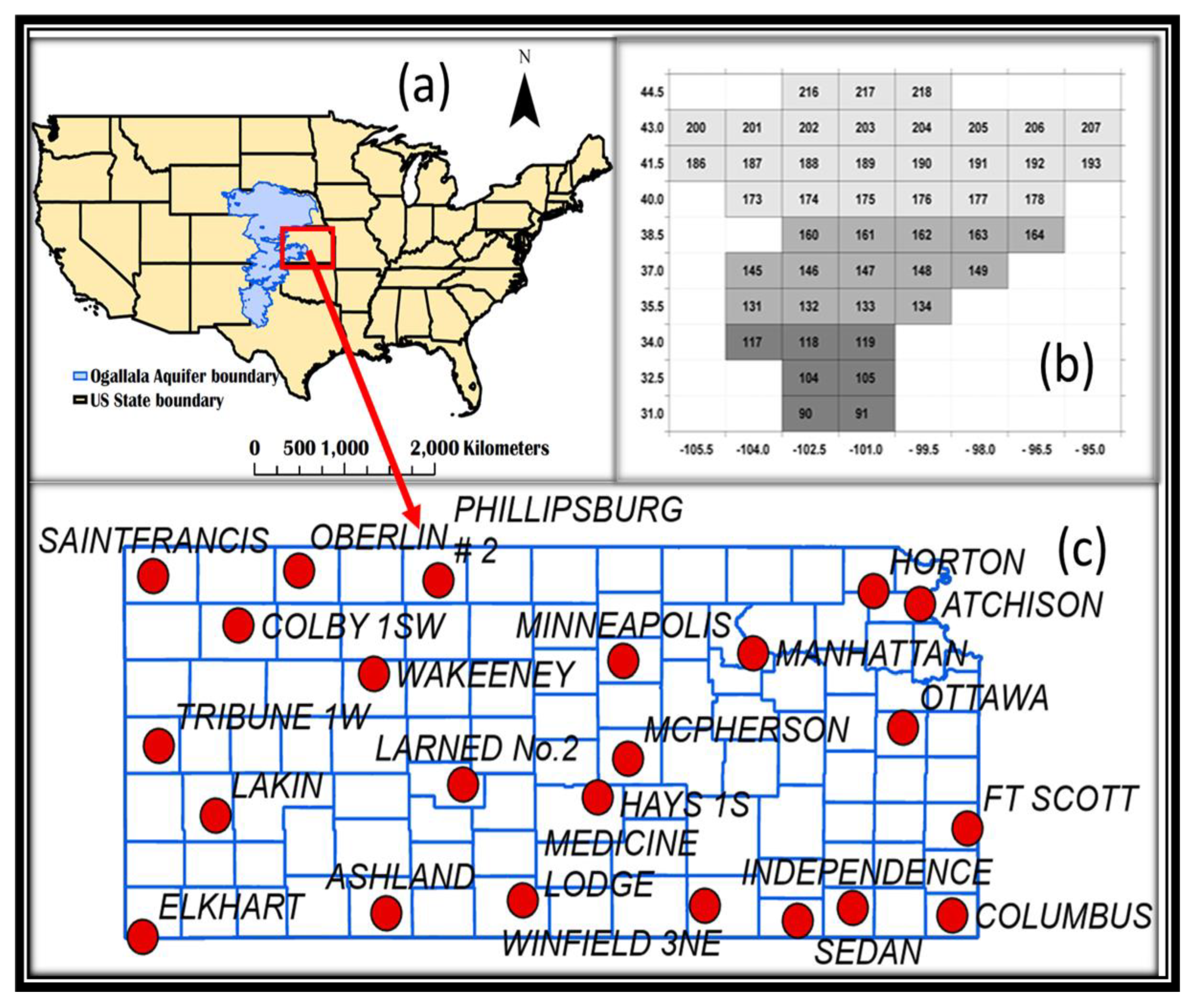
Step 1: Synthesize linear trends in agroecological indicators. This involves using the agro-ecosystem indicators trend data taken from Anandhi [6,26,33,34]. The details of the estimated trends can be found in them. The agro-ecosystem indicators––namely Crop Failure Temperature (CFT), Frost Indices–Last Spring Freeze (LSF), Frost Days (nFD) and First Fall Freeze (FFF), wet and dry spells, consecutive wet and dry days, warm and cold spell days––are used in the analysis. The CFTs for various crops grown in Kansas (30 °C, 35 °C, 39 °C, and 40 °C) are taken from Hatfield et al. 2008 and Herrero and Johnson, 1980. To evaluate the annual trends in agro-ecosystem indicators, the daily maximum air temperatures (Tmax) and minimum air temperatures (Tmin) were taken from the High Plains Regional Climate Center (HPRCC) for the period 1920–2009. The location of the study region is provided as a red rectangular box in Figure 1a. The meteorological stations used for the analysis are provided in Figure 1c.
Step 2: The study period is divided into three sections 1921–1950, 1951–1980, and 1981–2009 and the trends are either short-term trends (sample size ~30 years) or long-term trends (sample size ~90 years). The detailed steps of the methodology can be obtained from [25].
Step 3: Scenario funnel plots. These trends were imported as Excel files into the Python Jupyter Notebook and plotted as scenario lines using the iloc () function. The scenario funnels were developed based on linear trends. The width of the funnel mouth represents the spread of trends. Typically, narrower funnels represent less spread in the trend values. The details of the scenario funnel can be found in Anandhi [35,36].
3. Results and Discussion: Framework Application
3.1. Changes in Temperature and Precipitation Observed from Literature in the Region
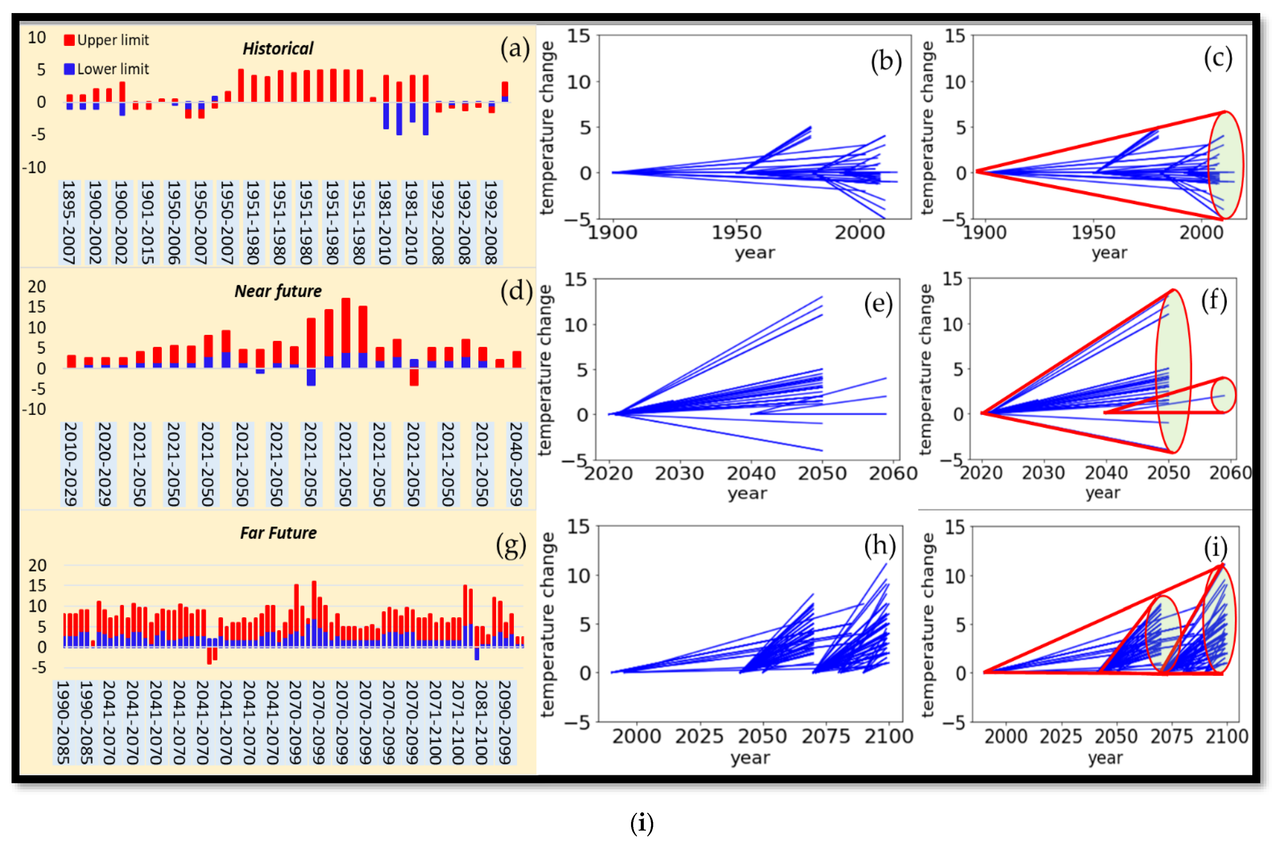
The meta-analysis involved studies related to changes in temperature (Figure 2i) and precipitation (Figure 2ii) over the Ogallala Aquifer region and their potential impacts on agriculture and ecosystem services. The data are divided into historical, near future, and far future data for ease of representation. Figure 2ia,d,h represent the bar plots of the temperature changes from the 18 studies. The change in values was only observed in the bar plots. The period of the changes was identified from the scenario plots in Figure 2ib,e,h. The temperatures varied from −4 °C to 8 °C. Historical models suggested a symmetrical steady shift from −2 °C to +2 °C from 1900 to 2000. Temperatures rapidly rose by up to 5 °C, between 1980 and 2000. The spread of the scenario lines was more biased towards positive temperature changes after 2000. The scenario lines also showed that the number of values increased. This suggested that there was an increase in the number of studies related to climate change in the aquifer region. A rapid increase in temperature was observed in future projections (Figure 2ih) until 2100 [37,38,39].
Precipitation had similar variability between 1900–2000. The changes in precipitation were symmetrical and gradual, although a negative change in precipitation values was observed between 1950–2000 (Figure 2iib,c). Future projections show a symmetrical spread of scenario lines. The precipitation changes for the near future period (2020–2050) show less spread with negative values (Figure 2iie,f). The precipitation changes from the 1990s to 2075 showed widespread variability compared with the temperature projections (Figure 2iih). The studies showed that the precipitation changes converged to a typical value (Figure 2iih,e).
3.2. Changes in Temperature and Precipitation from Data Analysis from Observations and Simulations
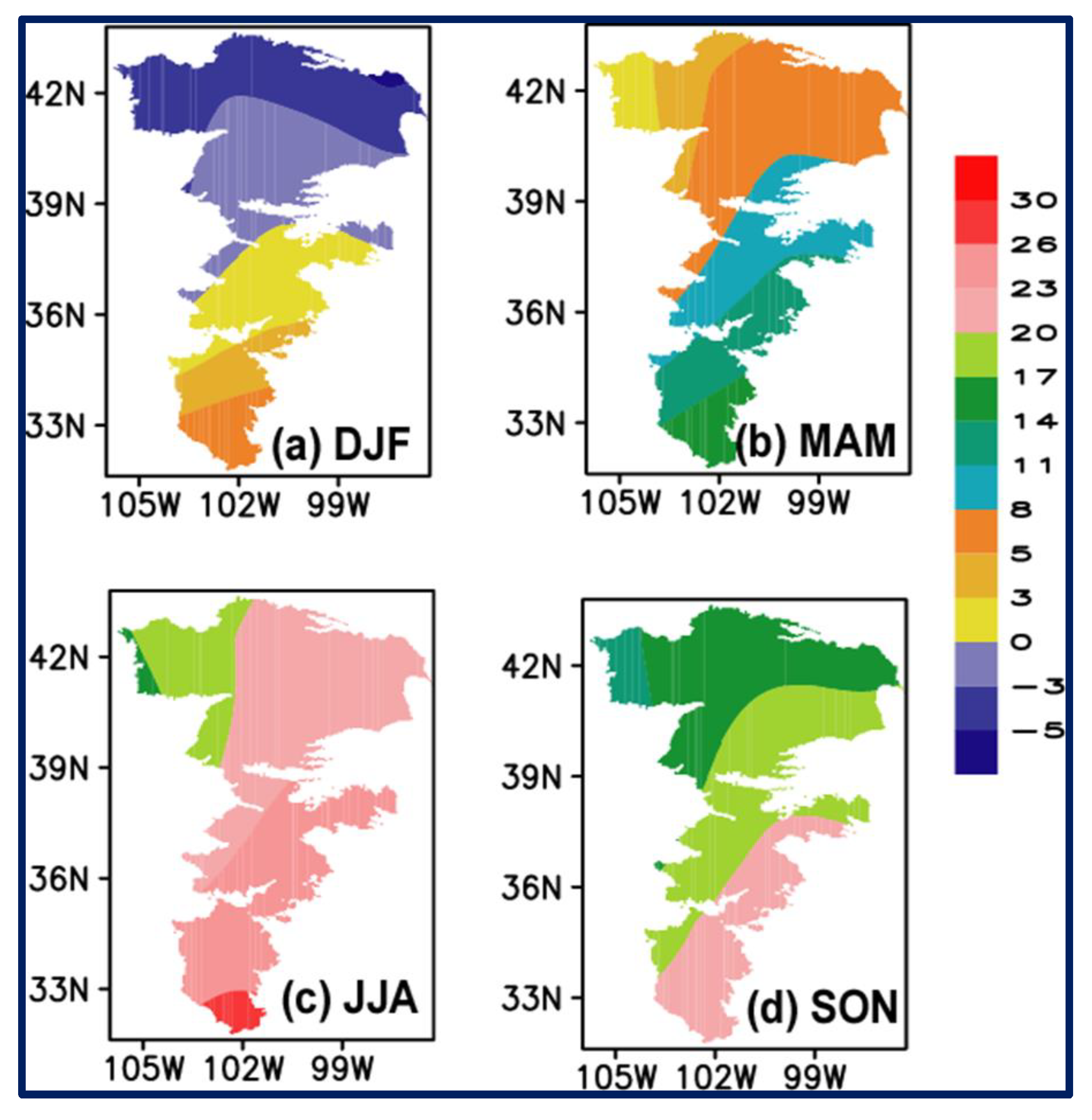
The observed temperature distribution (Figure 3) in the Ogallala Aquifer Region represents warming over the south and cool temperatures in the north during different seasons between 1971–2005. In general, a southeast-northwest seasonal temperature gradient is observed over the region, except in winter. The winter temperatures are characterized by ≤7 °C in the south and ≤−4 °C in the north, with a negative meridional temperature gradient (Figure 3a). The spring temperatures in the south were higher than the north (≤14 °C vs. ≤3 °C, respectively) (Figure 3b). The summer temperatures (Figure 3c) were between 18–27 °C. Similar features, such as summer, also occurred during the fall season (Figure 3d). Temperature distribution affects soil moisture over the region, and ultimately affects agriculture. Changes in soil moisture can lead to drought; this requires more irrigation in parts of the aquifer and leads to unsustainable water resources in the region [40].
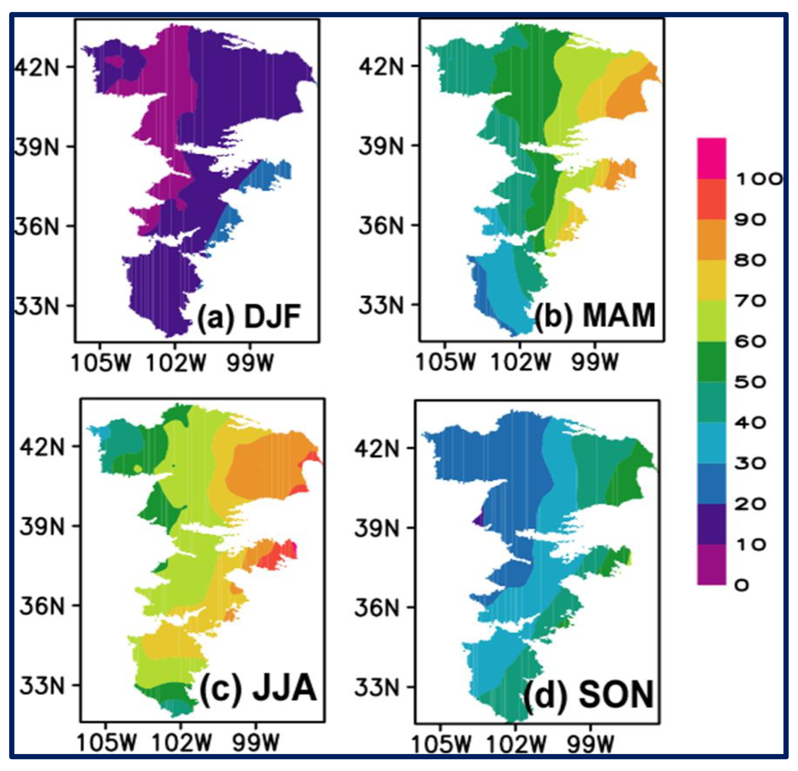
The precipitation distribution depicts a seasonal east-west gradient. High seasonal precipitation values are observed in the northeast region of the aquifer, except in winter Precipitation was high in the central-eastern part of the aquifer in all seasons, whereas the north-south gradient had low precipitation values during summer. Thus, the eastern region of the aquifer has the maximum precipitation during most seasons, while the western part of the aquifer requires irrigation. This results in greater water extraction from the aquifer, aquifer depletion, and a disturbance of the aquifer water balance. The precipitation values ranged from 95–45 mm in summer. The zonal distribution of precipitation in the northern sector of the aquifer marks a westward increase in precipitation from winter until summer, followed by a decrease in fall. The southern region of the aquifer has characteristically high precipitation values during fall compared to that of other seasons.
There is seasonal variability in addition to interannual variability in precipitation over the aquifer. This can create a more significant challenge for managing uncertainty in the agricultural sector and affect the adaptation time for responding to risks [41]. The need to switch to less water-sensitive crops is due to changes in precipitation and water availability.
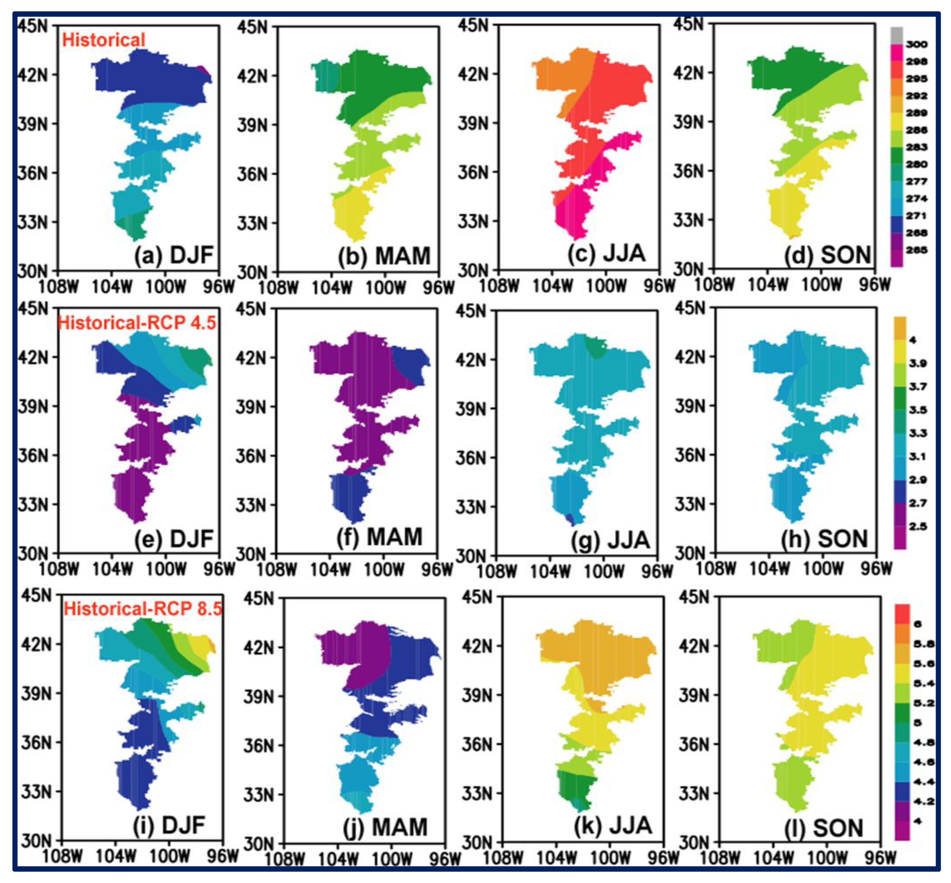
The observed climatological temperatures are provided in Figure 4. The observations showed a similar seasonal trend over the region as model simulations in Figure 5. Historical simulations from the models represent warming over the southern plains region in all seasons. The summer season is the warmest from the central region to the south, while cooling is observed in the northwest region of the aquifer (Figure 5a–d). These characteristics were consistent with the observed temperature distributions shown in Figure 3. The RCP4.5 future scenario (Figure 5e–h) indicated that the temperature anomalies (difference between RCP4.5 and historical) display warming in the northern region of the aquifer in all the seasons and cooling for the southern areas, except in spring (Figure 5f). The RCP8.5 scenarios (Figure 5i–l) present a similar pattern. However, the magnitude of the temperature anomalies were higher in RCP8.5.
The immediate effect of temperature increase is the likelihood of an increased reduction in soil moisture leading to drought conditions over the aquifer region from increased evapotranspiration. Many studies suggest that subtropical and temperate regions are likely to become drier at the expense of wetter tropics [2,3]. Climate predictions and observed data revealed that freshwater resources are vulnerable, and will be affected in the future [42]. This has long-lasting consequences for agro-ecosystems and society. Moreover, it influences the recharge capability of the aquifers [43]. Climate projections indicate an increase in temperature in the future; however, a proportionate increase in precipitation is not observed (see below).
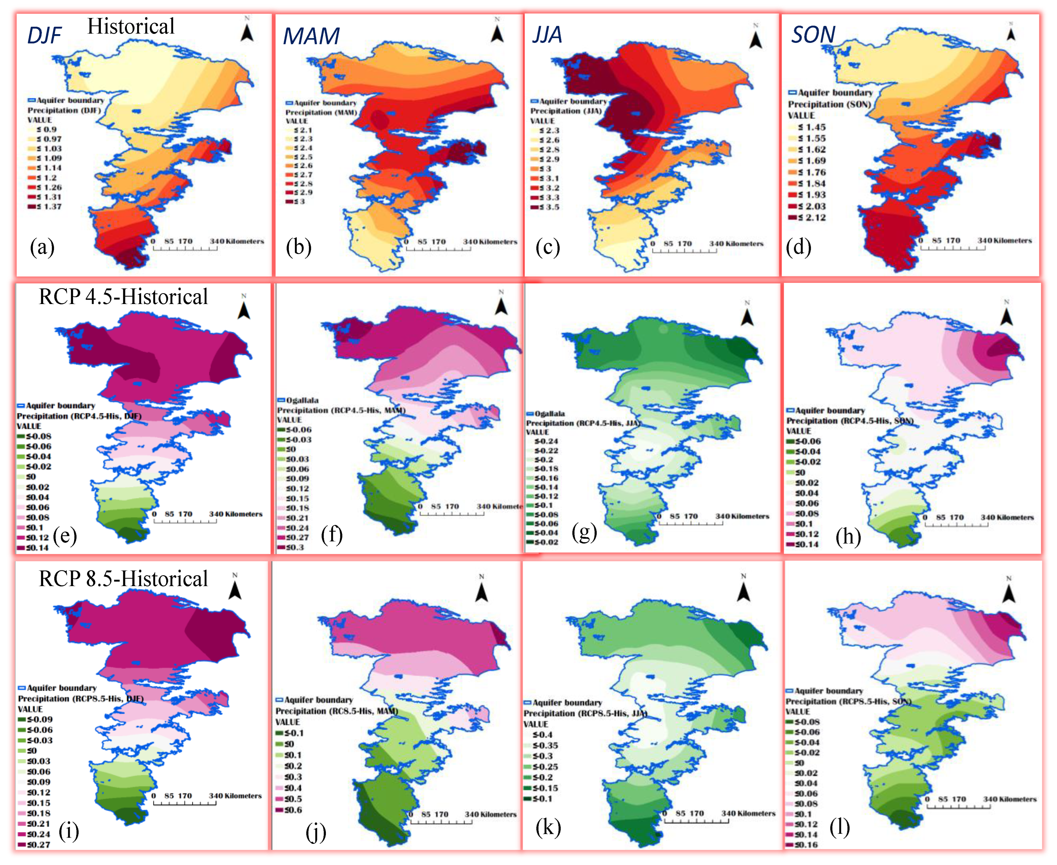
The historical seasonal ensemble means of precipitation for the period 1971–2005 are shown in Figure 6a–d. The precipitation pattern demonstrated a transition from low values in winter to high values in summer, followed by a decrease in fall. The fall and winter precipitation patterns (Figure 6a,d) show higher values in the central and southern portions of the aquifer. In contrast, spring and summer had higher values in the central and northern parts of the region (Figure 6b,c). The maxima are found in the central north region of the aquifer: northwest Colorado, northwest Kansas, and southwest Nebraska. The difference in precipitation between the historical simulations and RCPs (4.5, 8.5) between 2006–2099 is provided in the middle and right panels. Future projection anomalies in precipitation for RCP4.5 show positive values in the north in all seasons, except in summer. The summer season is characterized by decreasing precipitation (negative values) throughout the aquifer, specifically in the central aquifer regions encompassing Colorado, Kansas, and Oklahoma states. A difference in intensity is observed despite the higher future scenario (RCP8.5) projecting the same characteristics compared to RCP4.5. The shift in precipitation from the historical information to the future projection influences diffuse recharge, the dominant type of recharge in the Northern High Plains Aquifer region [43]. The fall season precipitation projection showed a decrease from Southern Texas to Southwest Kansas. Therefore, it was concluded that future summers over the Ogallala region will face water scarcity. This can disturb agricultural production and lead to food insecurity.
3.3. Changes in Agro-Ecosystem Indicators for Kansas
3.3.1. Crop Failure Temperature
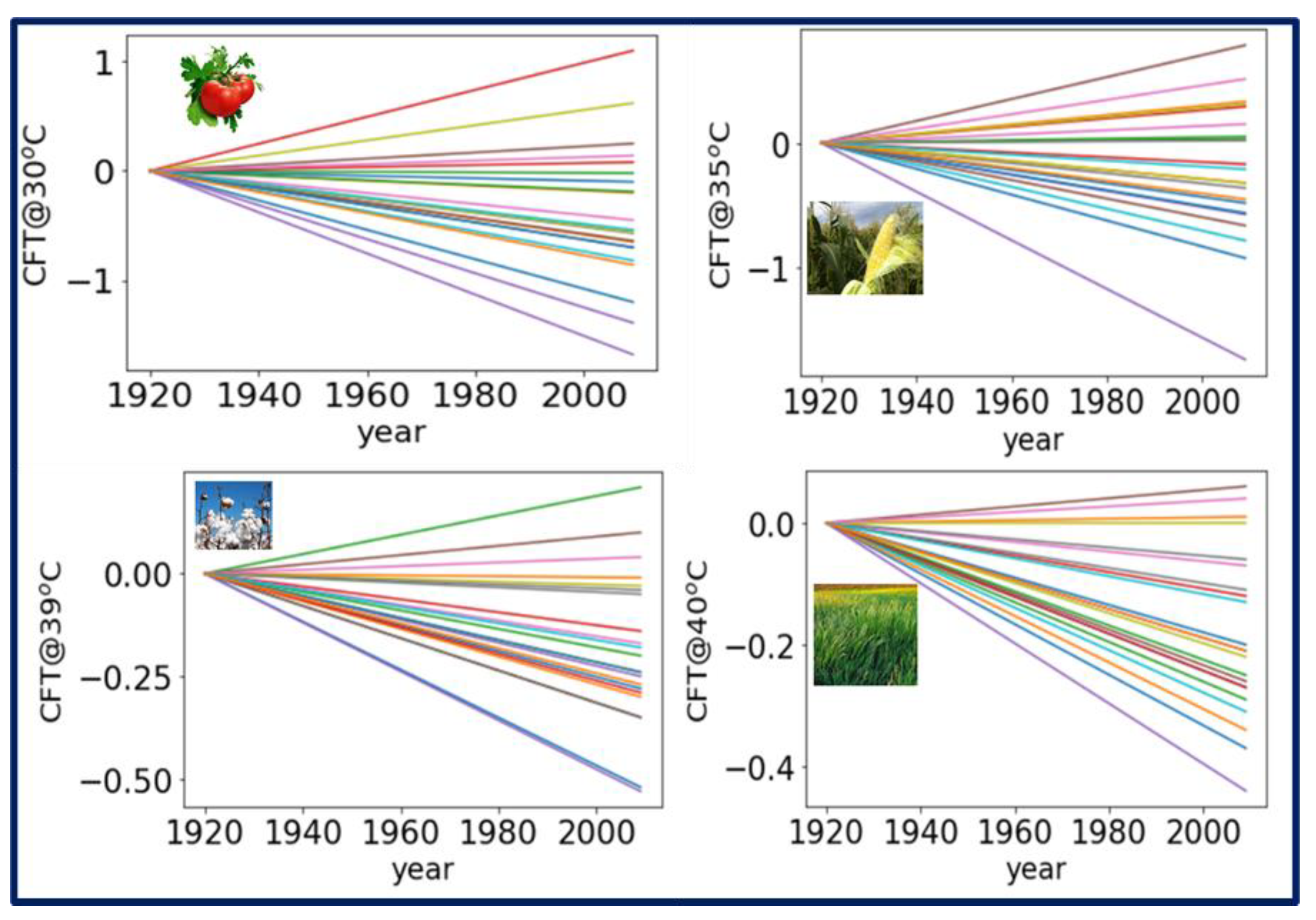
The linear trends in the number of days with CFT at 30 °C, 35 °C, 39 °C, and 40 °C for long- and short-term periods were taken from [33]. The long-term trends were chosen for the period between 1920–2010 (Figure 7). Most Kansas stations showed negative trends over the long-term period. The frequency of stations exhibiting negative trends was higher for CFT at 30 °C and 40 °C. However, the stations showed positive trends for CFT at 35 °C and 39 °C; this indicated more heat stress. The rise in average temperature increases the rates of crop development and evapotranspiration [44,45].
Short-term trends are classified into three periods: 1920–1950, 1951–1980, and 1981–2010. The scenario lines for the short-term trends between 1920–1950 portray a dominating positive trend for CFTs at 35 °C, 39 °C, and 40 °C (Figure 8). The stations exhibited positive and negative trends at 30 °C. The 1951–1980 period marks a bias towards more negative trends at 35 °C, 39 °C, and 40 °C. The trends for the CFT at 30 °C have positive and negative values. The trends show a maximum spread towards negative values for all CFTs after 1981. However, the maximum spread was towards positive and negative values for 30 °C and 35 °C CFTs. The values ranged from −12.5 to 5.0. The CFT at 40 °C is similar to that at 39 °C. Thus, the trends at different CFTs indicate that each crop species has a different temperature range for its growth stages. The response of temperature extremes above or below a certain threshold affects plant productivity [46]. The increase in temperature to a specific point creates excess energy in plants; however, elevation to very high temperatures retards plant growth and photosynthesis [47]. The use of CFT as an indicator of the discernible impacts of climate change can be useful for vulnerability studies to evaluate climate stress affecting agricultural production [25,48]. The use of CFT provides information to address crop productivity in relation to heat stress and high average temperatures. The most vulnerable plant process to elevated temperatures is flowering or anthesis during the reproductive stage [49]. Temperature stress (heat stress) alters pollen germination in maize. Temperature sensitivity is determined by the ideal temperature of a plant for growth and reproduction [45].
3.3.2. Frost Indices
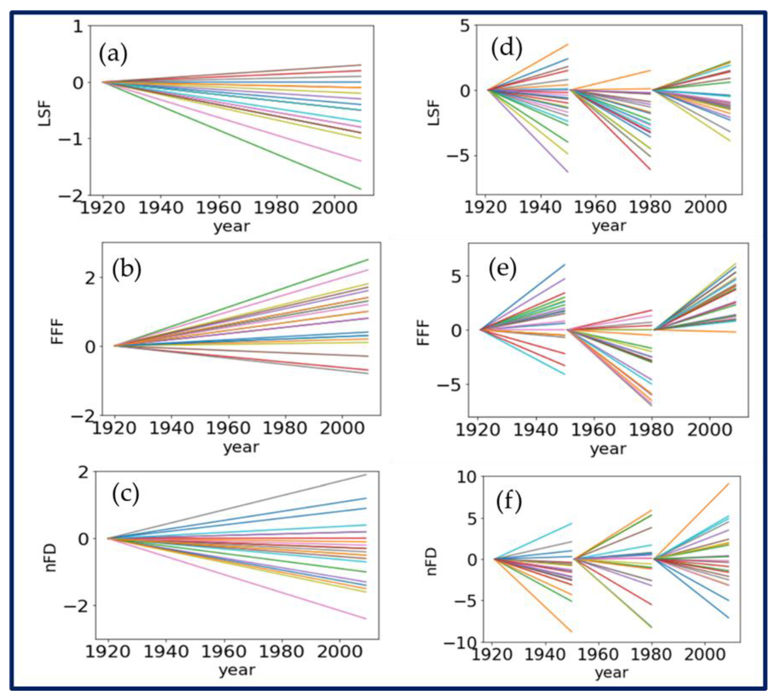
The scenario lines for the long-term linear trends offor the frost indices isare presented in Figure 9a–c. There is trends an overall negative trend for the day of the lLast sSpring fFreeze (LSF) have an overall negative trend (Figure 9a). Meanwhile On the other hand, the long-term trends oin the day of the fFirst fFall freeze (FFF) displayed positive trends for nearly 50% of the stations (Figure 9b). The number of frost days displayed negative trends at mostmajority of stations (Figure 9a). The trends in frost indices affect the length of the growing season length, and the LSF affects the sowing and FFF during the harvest season [25]. HThe harvesting depends on the crop variety, and it varies with climate. In Kansas, the average LSF days areis from the April first week in the sSoutheast region to the May first week in the nNorthwest region (Weather Data Library, KSU). Similarly, FFF starts from the second week of September in the nNorthwest region to the last week of October October last week in the southeast region.
The scenario lines for the short-term trends are shown in Figure 9d–f. Similar tTrends were observed forin LSF, FFF, and the the Nnumber ofno. of frost days for the stations exhibited a similar pattern during 1921–1950. The 1951–1980 decades 1951–1980 display a negative bias in trends for LSF (Figure 9d) and FFF (Figure 9e), with both positive and negative trends for the number of frost days (Figure 9f). The spread of the trend lines islines is symmetrical betweenin the recent period, 1981–2009 for the LSF. Most stations showed positive trends fForWhile for the FFF, most of the stations showed positive trends. The linear trend rangeds from −6 to 2.8. The scenario lines did not vary in the case of the number of fFrost dDays (nFD), whereaswhile the FFF showeds the most variability. An interesting featureT he spread of ofnoticed from the short-term trend liness for the LSF is that the spread of trend lines decreasedecreaseds between thefrom the 1920s to the 2000s. SimultaneouslyMeanwhile, atheAt the same time the reverse feature is observed for nFD. The synoptic drivers of freeze initiation events and atmospheric low- frequency oscillations maymight influence the FFF over the stations. Short-term trends of FFF short- term trends haves a maximum of 6.0 and a minimum of −6.0. Frost can affect the crops at the cellular level, tha by t causinges ice crystals formation between plant cells; this that triggers physical damage and atalso on certain life stages and. It can cause seedling mortality, also known as the ‘frost desert’, through frost heaving (vertical needle ice crystals) and frost thrusting (lateral ice crystals).
3.3.3. Wet and Dry Spell Indices
The annual long-term wet spell length (WSL) trend features positive values for most of the stations in Kansas. This indicated surplus water over the region (Figure 10a). Precipitation occurs in the form of rain or snow. The annual long-term dry spell length (DSL) shows a decreasing trend (Figure 10b). This indicated that dry spells have decreased over time in most locations
The annual WSL short-term trends were between −0.3 to 0.8 from 1920–1950. A bias towards negative values (decreasing wet spells) was observed from 1951–1980. Meanwhile, there was a decrease in spread and a shift towards negative values at most stations during 1981–2009. In contrast, the DSL short-term trends between 1920–1950 showed negative trends for most of the stations. The second period (1951–1980) depicts both positive and negative trends. The spread of the scenario lines decreased during 1981–2010, and the stations show positive and negative trends that point towards episodes of excess and scarce rainfall over the region. The scarcity of rainfall resulted in more irrigated areas in the region in recent decades. The WSL and DSL indicators help in agricultural planning and conservation of water and soil resources [50].
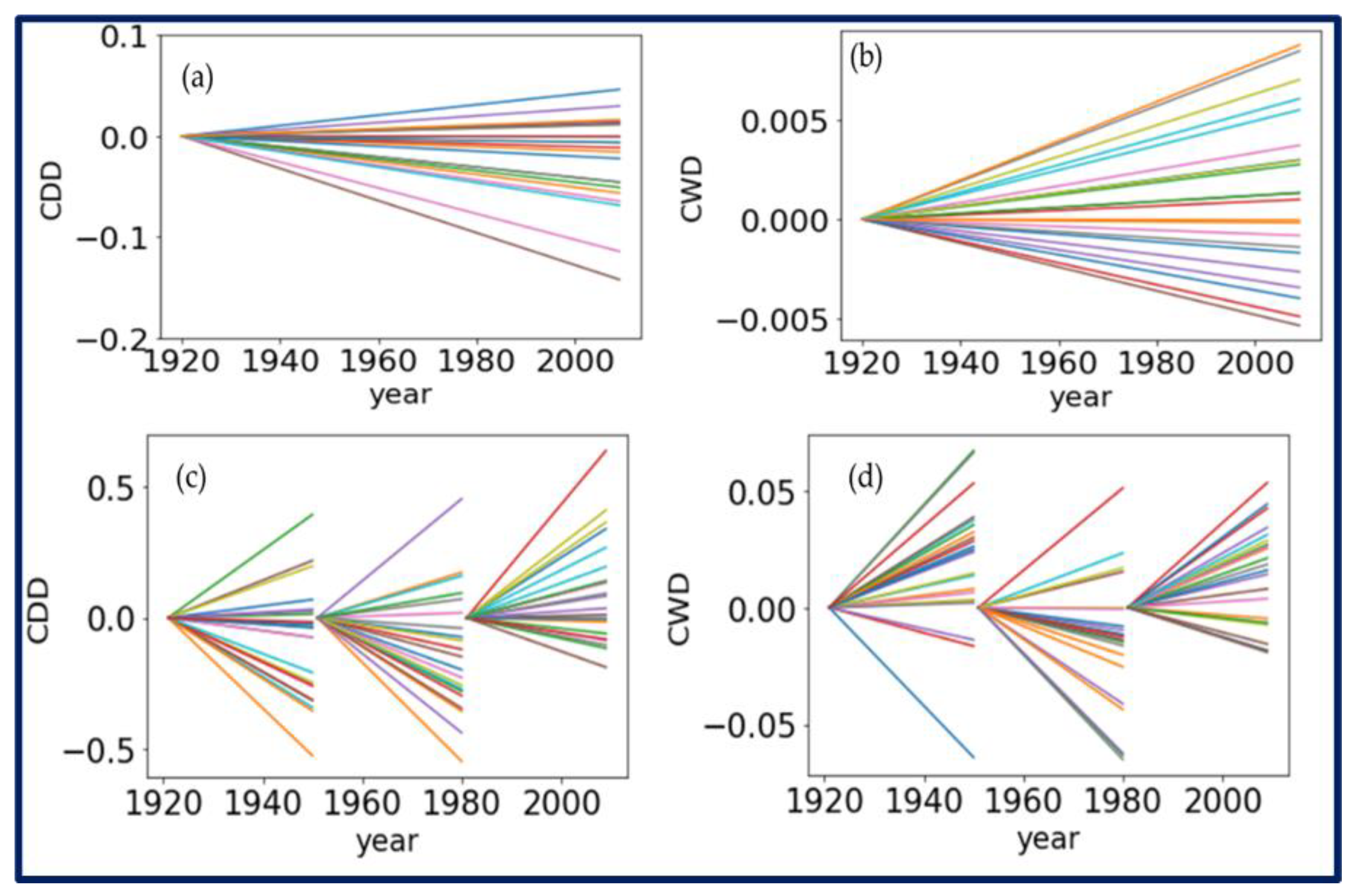
The long-term trends for the entire time period (1920–2009) show that the majority of stations have negative values for the number of consecutive dry days and for the consecutive wet days (Figure 11a,b). Therefore, there are no consecutive wet days contributing to the positive trend in the wet spell length (Figure 10), but there may be intermittent rain spells. The annual consecutive dry days for the three time periods characterized widespread negative trends between 1921–1950. Most of the stations were skewed towards negative trends during 1951–1980. The 1981–2009 period had a positive bias, with an increase in the number of consecutive dry days over the region. In contrast, the trends in consecutive wet days between 1921–1950 converged together with less spread with a symmetric structure. The 1951–1980 period had high negative values for all stations in the study domain, whereas the 1981–2009 period features similar trends to that of consecutive dry days (Figure 11c,d). The consecutive dry days (CDD) and annual consecutive wet days (CWD indicators provide an inference for crop planting or sowing under rainfed or irrigation conditions.
3.3.4. Warm and Cold Spell Indices
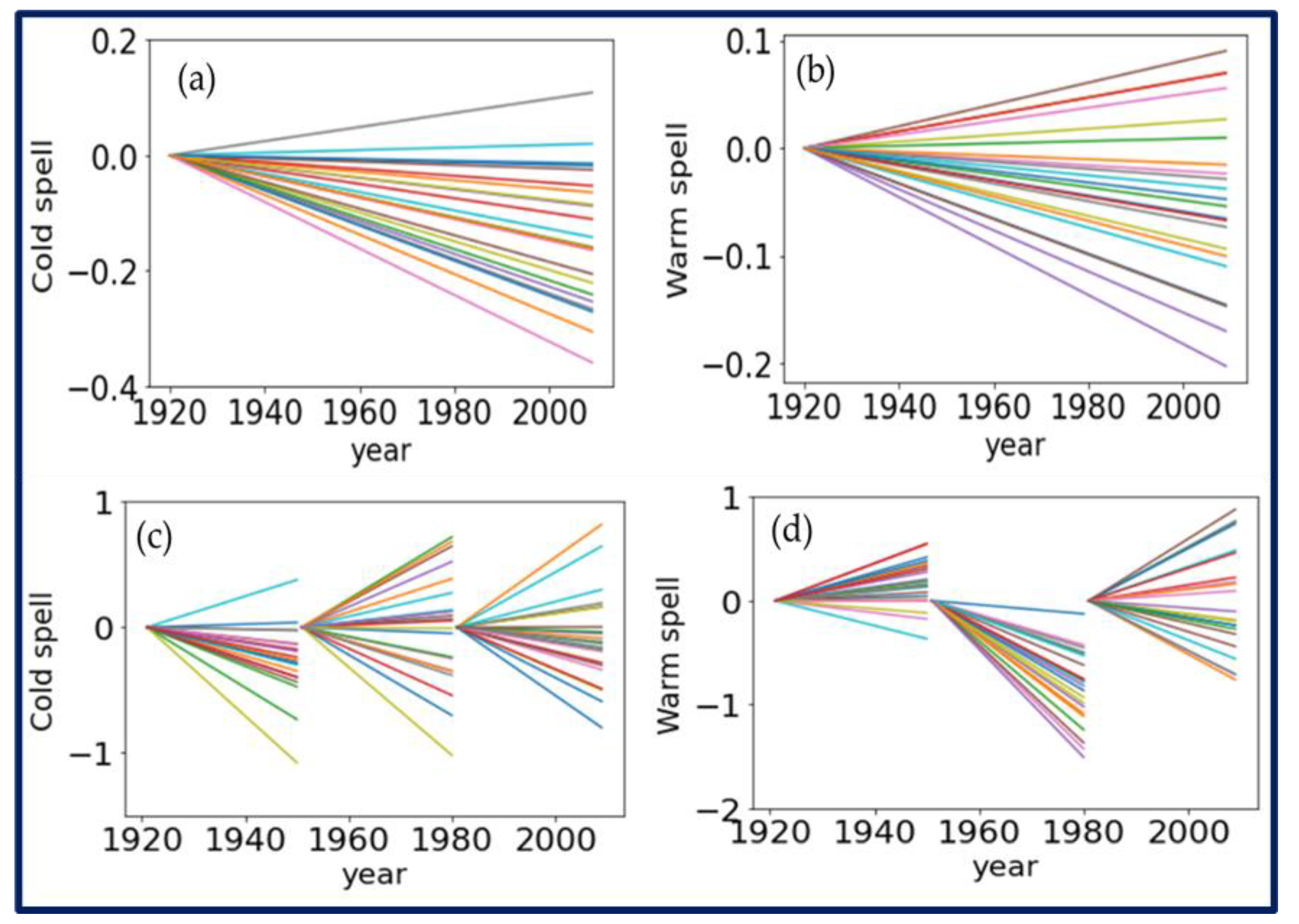
The annual cold spell days had more bias towards negative trends, even though some stations showed positive values. Warm spell days showed very weak positive trends compared with cold spells, but the negative bias was stronger. The annual cold spell days during 1921–1950 showed a bias towards negative trends. A symmetrical spread was observed between 1951–1980 and the later period represented positive and negative trends for the stations (Figure 12c). The majority of stations showed a positive trend of warm spell days (1921–1980) and negative trends for all stations between 1951–1980. The latter period (1981–2009) had warm spell day trends that were similar to that of the cold spells (Figure 12d).
4. Discussion
The focus of this study was to understand future climate projections in the Ogallala aquifer region using CMIP5 model projections. In addition, station-based agro-ecosystem indicators for the Kansas state and Central High Plains aquifer region were studied in detail to understand the effect of temperature and precipitation on agricultural crops.
4.1. Climate Model Predictions
Climate projections from meta-analyses (agro-meteorological indicators) and data analyses (CMIP5 models) show that climate change is already happening at a faster pace over the Ogallala aquifer region; this may impact the water resources over the region. The High-plain aquifer region has a mid-latitude dry continental climate with abundant sunshine, moderate precipitation, and a higher rate of evaporation. The location of a region determines the agronomically effective part of the growing season [51]. Agricultural production is directly vulnerable to temperature changes through crop growth and development, even though only a part of the growing season is used for food, feed, and biomass production. An increase in the frequency of extreme precipitation events, prolonged severe drought episodes, and an increase in temperature pose challenges for the US southern plains agricultural sector [41].
The CMIP5 model projections for temperature showed warming over the northeast region of the aquifer for all seasons. This affects the quality and productivity of feed crops, and poses an indirect health risk to animals. The precipitation estimates suggest a rise in the north and northeast during spring, summer, and winter. The early growing crop season is affected by changes in precipitation that are above normal. The impact of above-average precipitation depends on soil type, soil compaction, and soil management [52].
Summers will be substantially warmer, with less precipitation under the medium- and high-emission scenarios. This creates water stress that accelerates water demand. The global Aqueduct database [53] projects a 1.4–2 times increase in water stress over the Kansas region of the aquifer between 2030–2040. Large stretches of crops across the Great Plains, such as cotton, sunflower, soybean, and winter wheat, are rain-dependent (NOAA, 2015). The local climate is a major factor in determining water availability resources in a region. Soil quality is also at risk since changing temperature and rainfall patterns affect erosion and soil organic matter decomposition rates [54].
4.2. Potential Impacts and Decision-Making in Various Ecosystem Services
The temperature change in the range of −4 °C to 8 °C and precipitation change in the range of −50% to +50% over the Great Plains aquifer region can be used to create several scenarios important for decision making. These changes have important implications for ecosystem services by altering the equilibrium of the region and affecting the components of the system. For example, increasing temperature scenarios delay the onset of FFF and hasten the occurrence of LSF, increase the growing season length and the number of warm days. A warmer, longer growing season changes the distribution of plants grown within the region [55]. The decrease in precipitation increases the dry spells and may reduce the stream flow over the aquifer region; this can directly affect the groundwater. An increase in the number of extreme temperature events (high daytime highs or nighttime lows) and dry spells increases plant stress. These events impact Playa lakes and can result in a decline in groundwater levels over the region. Playas of the High Plains that are potential point sources of recharge to the High Plains aquifer provide wildlife habitats and help maintain regional biodiversity [56]. Declining groundwater levels lower the profitability of irrigation, leading to fewer irrigated acres and shifting to dryland farming. This shift has had negative consequences for agricultural producers and rural communities [57]. These socio-economic changes need to be incorporated into planning adaptation strategies to sustain ecosystem services, meet desired production, and accomplish conservation goals. Education and extension services are required to transfer adaptive knowledge in a timely manner to stakeholders in the field.
Climate-driven changes can significantly affect ecological flow regimes [58], and influence the cycling of nutrients which alters water quality [59]. Best management practices are required for effective water management and crop productivity, owing to the low recharge rate of the aquifer [60]. Increased high precipitation events can cause excess nutrient loading to the water bodies, leading to water quality degradation, including groundwater contamination, algal blooms, hypoxic/anoxic conditions, and the loss of fish biomass and native fish species, resulting in environmental costs. Scenarios of increasing precipitation in the region will be useful in the United States Department of Agriculture Conservation Reserve Program (CRP). This is a voluntary program that pays farmers to take environmentally susceptible croplands and change the land cover grassland, woodland, or wetlands for 10 to 15 years to achieve environmental benefits such as erosion reduction, surface water quality, and wildlife habitat benefits [61]. These shifts affect the migration pattern of fauna, species extinction, and so on [62].
4.3. Potential Impacts in Agricultural Production
Extreme temperatures and precipitation may reduce crop yields because of the reduction in water availability for agricultural production. A reduction in the water table increases the cost of pumping water. Farmers realize that dryland farming is the most cost-effective alternative that also saves the remaining irrigation water [63]. Therefore, there is a transition from irrigation-deficient regions to drylands for crop production, as outlined in recent studies [64,65,66]. However, land use planning at community and local scales must account for the likelihood that irrigated farmland would be converted to non-irrigated pasture agriculture rather than dryland crop cultivation; this has significant impacts for the environmental and the economy [65].
Scenarios of higher temperatures and dry spells impact the crop growth stages, and can be combined with water availability to (1) estimate changes in crop water requirement and potential evapotranspiration, (2) improve water use, especially during critical development stages, and (3) select hybrids that produce optimum yields in the anticipated scenarios [6,33,34,67]. Scenarios of increasing dry spell length can lead to prolonged droughts and increased irrigation requirements, resulting in decisions such as increased groundwater use, more drought-resistant crop varieties, or switching the cropping system to dry land. These decisions can alter the recharge rates of groundwater during the transition between irrigated and dry-land agriculture.
Frost is considered a major meteorological factor that impacts agriculture [68,69] in temperate and subtropical regions [68] and determines crop habitat. Therefore, scenarios of low temperature can be used to (1) study chill injury: this threatens crops by inducing ice crystals in tissues that affect growth and decrease yield; (2) estimating the impacts on crop physiology, specifically growth stages; (3) understanding the impact of freeze stress on the crop lipid phase transition temperature, lipid phosphate (lipid-P), free fatty acid levels, and formation of oxygen free radicals; (4) understanding hydrologic-, ecosystem-, and biogeochemical processes with changes in net primary productivity and evapotranspiration; and (5) studying frost impacts, the biochemical and physiological aspects of plants, and the complex process being named as frost hardening [26,34,70]. Frosts with winter precipitation affect water runoff, contribute to soil erosion, and nutrient leaching. Autumn-sown crops are sensitive to harsh winter conditions.
5. Conclusions
Several studies have documented climate change impacts on the region overlying the Ogallala Aquifer This is the first study to document temperature and precipitation changes over the entire Ogallala region from 35 General Circulation Models participating in phase 5 of the Climate Model Intercomparison Project (CMIP5), together with the development of agro-hyro meteorological indicator-based scenarios that stakeholders can utilize in decision-making.
The meta-analysis depicts a temperature range from −4 °C to 8 °C over the Great Plains aquifer region from 1900 to 2100. Historical simulations from 1900 to 2000 show a symmetrical gradual change from −2 °C to +2 °C, and decadal changes (1980–2000) represent a rapid increase in temperature up to 5 °C. The future precipitation projections have a symmetrical spread. This indicates less variability compared to the temperature changes. The spatial variability of temperature from the CMIP5 model simulations shows cooling in the northern part of the aquifer and warming in the south for historical runs. Scenario RCP4.5 projects a north-south gradient in temperature with strong warming in the north to northeast region. The RCP8.5 scenario sets a much warmer pattern for all seasons. Meanwhile, historical precipitation simulations have a southeast to northwest gradient for RCP4.5, with winter, spring and fall precipitation maxima on the north side of the aquifer. Summer precipitation is projected to be very weak. The higher emissions scenario projects that the central region of the aquifer will be drier.
The agro-ecosystem indicators for the stations in Kansas represent the greatest changes in the number of CFT days (30 °C and 35 °C) during 1981–2009. The eastern stations show a considerable decrease in the number of days of CFTs at 39 °C and 40 °C. The long-term trends on the day of the last spring freeze showed a decrease, and the short-term trends increased after 2000. Short-term annual wet spell lengths decreased. This indicated a shortage of water over the Kansas region of the aquifer. The use of agroecosystem indicators helps in the development of new crop varieties that can adapt to climate change. This is beneficial to sustainable agricultural management in the context of aquifer depletion. The scenario line portrayal of agro-meteorological indicators helps decision-makers make use of climate science in two ways: 1. Identify the transition zone between adaptation and transition 2. Determine when to make transitions based on previous experiences of conditions and the degree of climate change.
We propose to utilize the CMIP6 multi-model climate simulations in decision making for the Ogallala Aquifer as a future study. This is because CMIP6 projections consider socio-economic scenarios and future land-use scenarios. Most current scientific studies are focused on the transition of irrigated to dryland cropping systems [63] (one of the objectives of the Ogallala Aquifer Program [60]). The use of CMIP6 is an added advantage for better adaptation and mitigation strategies to cope with climate shocks. However, local/regional crop modelling studies using decision support tools and observational field experiments are required to supplement climate model projections. In addition, innovations in technology and management must be introduced in other states encompassing the Ogallala Aquifer for sustainable irrigation, such as the Local Enhanced Management Area (LEMA) in Kansas, USA, [71]).
Author Contributions
Conceptualization, methodology, and writing—original draft preparation, A.A.; validation, writing—review and editing, all listed co-authors; formal analysis, authors of individual case studies; funding acquisition, A.A. All authors have read and agreed to the published version of the manuscript.
Funding
This research was funded by USDA-NIFA capacity building grants 2017-38821-26405 and 2022-38821-37522, USDA-NIFA Evans-Allen Project, Grant 11979180/2016–01711, USDA-NIFA grant No. 2018–68002–27920, United States Department of Agriculture (USDA-NIFA) to Florida A&M University through Non-Assistance Cooperative Agreement grant No. 58-6066-1-044 as well as National Science Foundation Grant No. 1735235 awarded as part of the National Science Foundation Research Traineeship and Grant No. 2123440. The authors would like to thank Robert J. Lascano, USDA, Lubbock, Texas, for providing the Ogallala Aquifer Program (OAP) article. Radley Horton, Lamont Research Professor, Lamont-Doherty Earth Observatory, Columbia University Earth Institute, and Dan Bader, Center for Climate Systems Research @ NASA GISS, Columbia Climate School, Columbia University in the City of New York, are acknowledged for support with the GCM datasets.
Data Availability Statement
The research was carried out using publicly available data and no new data were created.
Conflicts of Interest
The authors declare no conflict of interest. The funders had no role in the study design; collection, analyses, or interpretation of data; writing of the manuscript; or decision to publish the results.
References
- Zhang, J.; Felzer, B.S.; Troy, T.J. Extreme precipitation drives groundwater recharge: The Northern High Plains Aquifer, central United States, 1950–2010. Hydrol. Process. 2016, 30, 2533–2545. [Google Scholar] [CrossRef]
- Anandhi, A. CISTA-A: Conceptual model using indicators selected by systems thinking for adaptation strategies in a changing climate: Case study in agro-ecosystems. Ecol. Model. 2017, 345, 41–55. [Google Scholar] [CrossRef]
- Scanlon, B.; Reedy, R.; Gates, J. Effects of irrigated agroecosystems: 1. Quantity of soil water and groundwater in the southern High Plains, Texas. Water Resour. Res. 2010, 46, W09537. [Google Scholar] [CrossRef]
- Sanderson, M.R.; Frey, R.S. From desert to breadbasket… to desert again? A metabolic rift in the High Plains Aquifer. J. Political Ecol. 2014, 21, 517. [Google Scholar] [CrossRef]
- Burris, L.; Skagen, S.K. Modeling sediment accumulation in North American playa wetlands in response to climate change, 1940–2100. Clim. Chang. 2013, 117, 69–83. [Google Scholar] [CrossRef]
- Anandhi, A. Growing degree days–Ecosystem indicator for changing diurnal temperatures and their impact on corn growth stages in Kansas. Ecol. Indic. 2016, 61, 149–158. [Google Scholar] [CrossRef]
- Walthall, C. Climate change and agriculture in the United States: Effects and adaptation. USDA Tech. Bull. 2012, 1935, 1–186. [Google Scholar]
- Esnault, L.; Gleeson, T.; Wada, Y.; Heinke, J.; Gerten, D.; Flanary, E.; Bierkens, M.F.P.; van Beek, L.P.H. Linking groundwater use and stress to specific crops using the groundwater footprint in the Central Valley and High Plains aquifer systems, U.S. Water Resour. Res. 2014, 50, 4953–4973. [Google Scholar] [CrossRef]
- Multsch, S.; Pahlow, M.; Ellensohn, J.; Michalik, T.; Frede, H.-G.; Breuer, L. A hotspot analysis of water footprints and groundwater decline in the High Plains aquifer region, USA. Reg. Environ. Chang. 2016, 16, 2419–2428. [Google Scholar] [CrossRef]
- Mastrandrea, M.D.; Heller, N.E.; Root, T.L.; Schneider, S.H. Bridging the gap: Linking climate-impacts research with adaptation planning and management. Clim. Chang. 2010, 100, 87–101. [Google Scholar] [CrossRef]
- Crosbie, R.S.; Scanlon, B.R.; Mpelasoka, F.S.; Reedy, R.C.; Gates, J.B.; Zhang, L. Potential climate change effects on groundwater recharge in the High Plains Aquifer, USA. Water Resour. Res. 2013, 49, 3936–3951. [Google Scholar] [CrossRef] [Green Version]
- Zhang, Y.; Lin, X.; Gowda, P.; Brown, D.; Zambreski, Z.; Kutikoff, S. Recent Ogallala aquifer region drought conditions as observed by terrestrial water storage anomalies from GRACE. JAWRA J. Am. Water Resour. Assoc. 2019, 55, 1370–1381. [Google Scholar] [CrossRef]
- Sharda, V.; Gowda, P.H.; Marek, G.; Kisekka, I.; Ray, C.; Adhikari, P. Simulating the Impacts of Irrigation Levels on Soybean Production in Texas High Plains to Manage Diminishing Groundwater Levels. JAWRA J. Am. Water Resour. Assoc. 2019, 55, 56–69. [Google Scholar] [CrossRef]
- Steward, D.R.; Bruss, P.J.; Yang, X.; Staggenborg, S.A.; Welch, S.M.; Apley, M.D. Tapping unsustainable groundwater stores for agricultural production in the High Plains Aquifer of Kansas, projections to 2110. Proc. Natl. Acad. Sci. USA 2013, 110, E3477–E3486. [Google Scholar] [CrossRef]
- Gowda, P.; Bailey, R.; Kisekka, I.; Lin, X.; Uddameri, V. Featured Series Introduction: Optimizing Ogallala Aquifer Water Use to Sustain Food Systems. J. Am. Water Resour. Assoc. 2019, 55, 3–5. [Google Scholar] [CrossRef]
- Rudnick, D.R.; Irmak, S.; West, C.; Chávez, J.L.; Kisekka, I.; Marek, T.H.; Schneekloth, J.P.; Mitchell McCallister, D.; Sharma, V.; Djaman, K.; et al. Deficit Irrigation Management of Maize in the High Plains Aquifer Region: A Review. JAWRA J. Am. Water Resour. Assoc. 2019, 55, 38–55. [Google Scholar] [CrossRef]
- Zhang, T.; Lin, X. Assessing future drought impacts on yields based on historical irrigation reaction to drought for four major crops in Kansas. Sci. Total Environ. 2016, 550, 851–860. [Google Scholar] [CrossRef]
- Hoerling, M.; Eischeid, J.; Kumar, A.; Leung, R.; Mariotti, A.; Mo, K.; Schubert, S.; Seager, R. Causes and predictability of the 2012 Great Plains drought. Bull. Am. Meteorol. Soc. 2014, 95, 269–282. [Google Scholar] [CrossRef]
- Haacker, E.M.K.; Sharda, V.; Cano, M.A.; Hrozencik, R.A.; Nunez, A.; Zambreski, Z.; Nozari, S.; Smith, G.E.B.; Moore, L.; Sharma, S.; et al. Transition Pathways to Sustainable Agricultural Water Management: A Review of Integrated Modeling Approaches. JAWRA J. Am. Water Resour. Assoc. 2019, 55, 6–23. [Google Scholar] [CrossRef]
- Venkataraman, K.; Tummuri, S.; Medina, A.; Perry, J. 21st century drought outlook for major climate divisions of Texas based on CMIP5 multimodel ensemble: Implications for water resource management. J. Hydrol. 2016, 534, 300–316. [Google Scholar] [CrossRef]
- Maupin, M.A.; Barber, N.L. Estimated withdrawals from principal aquifers in the United States, 2000. In Geological Survey Circular; U.S. Department of the Interior and U.S. Geological Survey: Baltimore, MD, USA, 2005; Volume 1279, 46p, ISBN 0-607-96780-3 2005. [Google Scholar]
- Dutton, A.R.; Mace, R.E.; Reedy, R.C. Quantification of Spatially Varying Hydrogeologic Properties for a Predictive Model of Groundwater Flow in the Ogallala Aquifer, Northern Texas Panhandle. In Geology of the Llano Estacado: New Mexico Geological Society 52nd Annual Field Conference; New Mexico Geological Society: Socorro, NM, USA, 2001. [Google Scholar]
- Scanlon, B.R.; Gates, J.B.; Reedy, R.C.; Jackson, W.A.; Bordovsky, J.P. Effects of irrigated agroecosystems: 2. Quality of soil water and groundwater in the southern High Plains, Texas. Water Resour. Res. 2010, 46, WR008428. [Google Scholar] [CrossRef]
- Steward, R.D.; Bruss, P.J.; Yang, X.; Apley, M.D. Tapping Groundwater Stores for Agriculture. 2013. Available online: https://pubmed.ncbi.nlm.nih.gov/23980153/ (accessed on 18 January 2023).
- Anandhi, A.; Steiner, J.L.; Bailey, N. A system’s approach to assess the exposure of agricultural production to climate change and variability. Clim. Chang. 2016, 136, 647–659. [Google Scholar] [CrossRef]
- Anandhi, A.; Perumal, S.; Gowda, P.H.; Knapp, M.; Hutchinson, S.; Harrington, J.; Murray, L.; Kirkham, M.B.; Rice, C.W. Long-term spatial and temporal trends in frost indices in Kansas, USA. Clim. Chang. 2013, 120, 169–181. [Google Scholar] [CrossRef]
- Harris, I.; Jones, P.D.; Osborn, T.J.; Lister, D.H. Updated High-Resolution Grids of Monthly Climatic Observations—The CRU TS3.10 Dataset. Int. J. Climatol. 2014, 34, 623–642. [Google Scholar] [CrossRef]
- New, M.; Hulme, M.; Jones, P. Representing Twentieth-Century Space–Time Climate Variability. Part II: Development of 1901–96 Monthly Grids of Terrestrial Surface Climate. J. Clim. 2000, 13, 2217–2238. [Google Scholar] [CrossRef]
- Kalnay, E.; Kanamitsu, M.; Kistler, R.; Collins, W.; Deaven, D.; Gandin, L.; Iredell, M.; Saha, S.; White, G.; Woollen, J.; et al. The NCEP/NCAR 40-Year Reanalysis Project. Bull. Am. Meteorol. Soc. 1996, 77, 437–472. [Google Scholar] [CrossRef]
- Taylor, K.E.; Stouffer, R.J.; Meehl, G.A. An Overview of CMIP5 and the Experiment Design. Bull. Am. Meteorol. Soc. 2012, 93, 485–498. [Google Scholar] [CrossRef]
- Thomson, A.M.; Calvin, K.V.; Smith, S.J.; Kyle, G.P.; Volke, A.; Patel, P.; Delgado-Arias, S.; Bond-Lamberty, B.; Wise, M.A.; Clarke, L.E.; et al. RCP4.5: A pathway for stabilization of radiative forcing by 2100. Clim. Chang. 2011, 109, 77. [Google Scholar] [CrossRef]
- Goodman, L.A. Snowball sampling. Ann. Math. Stat. 1961, 32, 148–170. [Google Scholar] [CrossRef]
- Anandhi, A.; Blocksome, C.E. Developing adaptation strategies using an agroecosystem indicator: Variability in crop failure temperatures. Ecol. Indic. 2017, 76, 30–41. [Google Scholar] [CrossRef]
- Anandhi, A.; Hutchinson, S.; Harrington, J.; Rahmani, V.; Kirkham, M.B.; Rice, C.W. Changes in spatial and temporal trends in wet, dry, warm and cold spell length or duration indices in Kansas, USA. Int. J. Climatol. 2016, 36, 4085–4101. [Google Scholar] [CrossRef]
- Anandhi, A.; Omani, N.; Chaubey, I.; Horton, R.; Bader, D.; Nanjundiah, R. Synthetic scenarios from CMIP5 model simulations for climate change impact assessments in managed ecosystems and water resources: Case study in South Asian countries. Trans. ASABE 2016, 59, 1715–1731. [Google Scholar]
- Anandhi, A.; Sharma, A.; Sylvester, S. Can meta-analysis be used as a decision-making tool for developing scenarios and causal chains in eco-hydrological systems? Case study in Florida. Ecohydrology 2018, 11, e1997. [Google Scholar] [CrossRef]
- Pachauri, R.K.; Allen, M.R.; Barros, V.R.; Broome, J.; Cramer, W.; Christ, R.; Church, J.A.; Clarke, L.; Dahe, Q.; Dasgupta, P.; et al. Climate Change 2014: Synthesis Report. Contribution of Working Groups I, II and III to the Fifth Assessment Report of the Intergovernmental Panel on Climate Change; Intergovernmental Panel on Climate Change: Geneva, Switzerland, 2014. [Google Scholar]
- Liu, B.; Asseng, S.; Müller, C.; Ewert, F.; Elliott, J.; Lobell, D.B.; Martre, P.; Ruane, A.C.; Wallach, D.; Jones, J.W.; et al. Similar estimates of temperature impacts on global wheat yield by three independent methods. Nat. Clim. Chang. 2016, 6, 1130–1136. [Google Scholar] [CrossRef]
- Alexandru, A. Consideration of land-use and land-cover changes in the projection of climate extremes over North America by the end of the twenty-first century. Clim. Dyn. 2018, 50, 1949–1973. [Google Scholar] [CrossRef]
- Basso, B.; Kendall, A.D.; Hyndman, D.W. The future of agriculture over the Ogallala Aquifer: Solutions to grow crops more efficiently with limited water. Earth’s Future 2013, 1, 39–41. [Google Scholar] [CrossRef]
- Steiner, J.L.; Briske, D.D.; Brown, D.P.; Rottler, C.M. Vulnerability of Southern Plains agriculture to climate change. Clim. Chang. 2018, 146, 201–218. [Google Scholar] [CrossRef]
- Bates, B.; Kundzewicz, Z.; Wu, S. Climate Change and Water; Intergovernmental Panel on Climate Change Secretariat: Geneva, Switzerland, 2008; ISBN 978-92-9169-123-4. Available online: http://www.ecorresponsabilidad.es/pdfs/orcc/climate_change_and_water/02-front-matter.pdf (accessed on 18 January 2023).
- Meixner, T.; Manning, A.H.; Stonestrom, D.A.; Allen, D.M.; Ajami, H.; Blasch, K.W.; Brookfield, A.E.; Castro, C.L.; Clark, J.F.; Gochis, D.J.; et al. Implications of projected climate change for groundwater recharge in the western United States. J. Hydrol. 2016, 534, 124–138. [Google Scholar] [CrossRef]
- Stone, M.C.; Hotchkiss, R.S.; Hubbard, C.M.; Fontaine, T.A.; Mearns, L.O.; Arnold, J.G. Impacts of Climate Change on Missouri Rwer Basin Water Yield. JAWRA J. Am. Water Resour. Assoc. 2007, 37, 1119–1129. [Google Scholar] [CrossRef]
- Wahid, A.; Gelani, S.; Ashraf, M.; Foolad, M.R. Heat tolerance in plants: An overview. Environ. Exp. Bot. 2007, 61, 199–223. [Google Scholar] [CrossRef]
- Hatfield, J.L.; Prueger, J.H. Temperature extremes: Effect on plant growth and development. Weather. Clim. Extrem. 2015, 10, 4–10. [Google Scholar] [CrossRef]
- Tkemaladze, G.S.; Makhashvili, K.A. Climate changes and photosynthesis. Ann. Agrar. Sci. 2016, 14, 119–126. [Google Scholar] [CrossRef] [Green Version]
- Mendelsohn, R. What Causes Crop Failure? Clim. Chang. 2007, 81, 61–70. [Google Scholar] [CrossRef]
- Nakagawa, H.; Horie, T.; Matsui, T. Effects of climate change on rice production and adaptive technologies. Rice science: Innovations and Impact for Livelihood. In Proceedings of the International Rice Research Conference, Beijing, China, 16–19 September 2002; Volume 2003, pp. 635–658. [Google Scholar]
- Manikandan, M.; Gurusamy, T.; Bhuvaneswari, J.; Prabhakaran, N. Wet and Dry Spell Analysis for Agricultural Crop Planning Using Markov Chain Probability Model at Bhavanisagar. Int. J. Math. Comput. Sci. 2017, 7, 11–22. [Google Scholar]
- Peltonen-Sainio, P.; Pirinen, P.; Mäkelä, H.M.; Hyvärinen, O.; Huusela-Veistola, E.; Ojanen, H.; Venäläinen, A. Spatial and temporal variation in weather events critical for boreal agriculture: I Elevated temperatures. Agric. Food Sci. 2016, 25, 44–56. [Google Scholar] [CrossRef]
- Turunen, M.; Warsta, L.; Paasonen-Kivekäs, M.; Nurminen, J.; Alakukku, L.; Myllys, M.; Koivusalo, H. Effects of terrain slope on long-term and seasonal water balances in clayey, subsurface drained agricultural fields in high latitude conditions. Agric. Water Manag. 2015, 150, 139–151. [Google Scholar] [CrossRef]
- Luck, M.; Landis, M.; Gassert, F. Aqueduct Water Stress Projections: Decadal Projections of Water Supply and Demand Using CMIP5 GCMs; World Resources Institute: Washington, DC, USA, 2015. [Google Scholar]
- Bowling, L.C.; Widhalm, M.; Cherkauer, K.A.; Beckerman, J.; Brouder, S.; Buzan, J.; Doering, O.; Ebner, P.; Frankenburger, J.; Kladivko, E.J.; et al. Indiana’s Agriculture in a Changing Climate: A Report from the Indiana Climate Change Impacts Assessment; Purdue University: West Lafayette, IN, USA, 2018; Available online: https://docs.lib.purdue.edu/agriculturetr/1/ (accessed on 18 January 2023).
- Cano, A.; Núñez, A.; Acosta-Martinez, V.; Schipanski, M.; Ghimire, R.; Rice, C.; West, C. Current knowledge and future research directions to link soil health and water conservation in the Ogallala Aquifer region. Geoderma 2018, 328, 109–118. [Google Scholar] [CrossRef]
- Johnson, W.C.; Stotler, R.L.; Bowen, M.W.; Kastens, J.H.; Hirmas, D.R.; Burt, D.J.; Salley, K.A. Assessing Playas as Point Sources for Recharge of the High Plains Aquifer, Western Kansas. In Prepared for US Environmental Protection Agency and Kansas Water Office; Kansas Geological Survey Open-File Report; 2019; Volume 2. Available online: https://www.researchgate.net/profile/William-Johnson-57/publication/321415088_INVESTIGATION_OF_PLAYA_HYDROLOGY_AND_RECHARGE_FLUX_TO_THE_HIGH_PLAINS_AQUIFER_AT_EHMKE_PLAYA_IN_WESTERN_KANSAS/links/5e1f2375299bf17457c56a85/INVESTIGATION-OF-PLAYA-HYDROLOGY-AND-RECHARGE-FLUX-TO-THE-HIGH-PLAINS-AQUIFER-AT-EHMKE-PLAYA-IN-WESTERN-KANSAS.pdf (accessed on 18 January 2023).
- Larsen, A.E. Agricultural landscape simplification does not consistently drive insecticide use. Proc. Natl. Acad. Sci. USA 2013, 110, 15330–15335. [Google Scholar] [CrossRef]
- Havril, T.; Tóth, Á.; Molson, J.W.; Galsa, A.; Mádl-Szőnyi, J. Impacts of predicted climate change on groundwater flow systems: Can wetlands disappear due to recharge reduction? J. Hydrol. 2018, 563, 1169–1180. [Google Scholar] [CrossRef]
- Richter, B.D.; Mathews, R.; Harrison, D.L.; Wigington, R. Ecologically Sustainable Water Management: Managing River Flows for Ecological Integrity. Ecol. Appl. 2003, 13, 206–224. [Google Scholar] [CrossRef]
- Brauer, D.; Devlin, D.; Wagner, K.; Ballou, M.; Hawkins, D.; Lascano, R. Ogallala Aquifer Program: A Catalyst for Research and Education to Sustain the Ogallala Aquifer on the Southern High Plains (2003–2017). J. Contemp. Water Res. Educ. 2017, 162, 4–17. [Google Scholar] [CrossRef]
- Riley, D.; Mieno, T.; Schoengold, K.; Brozović, N. The impact of land cover on groundwater recharge in the High Plains: An application to the Conservation Reserve Program. Sci. Total Environ. 2019, 696, 133871. [Google Scholar] [CrossRef]
- Cameron, G.N.; Scheel, D. Getting Warmer: Effect of Global Climate Change on Distribution of Rodents in Texas. J. Mammal. 2001, 82, 652–680. [Google Scholar] [CrossRef]
- Lascano, R.J. Editorial: Transition From Deficit-Irrigated to Dryland Crop Production. Front. Sustain. Food Syst. 2021, 5, 707782. [Google Scholar] [CrossRef]
- Carr, P.M.; Bell, J.M.; Boss, D.L.; DeLaune, P.; Eberly, J.O.; Edwards, L.; Fryer, H.; Graham, C.; Holman, J.; Islam, M.A.; et al. Annual forage impacts on dryland wheat farming in the Great Plains. Agron. J. 2020, 113, 1–25. [Google Scholar] [CrossRef]
- Deines, J.M.; Schipanski, M.E.; Golden, B.; Zipper, S.C.; Nozari, S.; Rottler, C.; Guerrero, B.; Sharda, V. Transitions from irrigated to dryland agriculture in the Ogallala Aquifer: Land use suitability and regional economic impacts. Agric. Water Manag. 2020, 233, 106061. [Google Scholar] [CrossRef]
- Chen, Y.; Marek, G.W.; Marek, T.H.; Porter, D.O.; Brauer, D.K.; Srinivasan, R. Modeling climate change impacts on blue, green, and grey water footprints and crop yields in the Texas High Plains, USA. Agric. For. Meteorol. 2021, 310, 108649. [Google Scholar] [CrossRef]
- Sharma, A.; Deepa, R.; Sankar, S.; Pryor, M.; Stewart, B.; Johnson, E.; Anandhi, A. Use of growing degree indicator for developing adaptive responses: A case study of cotton in Florida. Ecol. Indic. 2021, 124, 107383. [Google Scholar] [CrossRef]
- Snyder, R.L.; Melo-Abreu, J.P. Frost protection: Fundamentals, practice and economics. Volume 1. Frost Prot. Fundam. Pract. Econ. 2005, 1, 1–240. [Google Scholar]
- Papagiannaki, K.; Lagouvardos, K.; Kotroni, V.; Papagiannakis, G. Agricultural losses related to frost events: Use of the 850 hPa level temperature as an explanatory variable of the damage cost. Nat. Hazards Earth Syst. Sci. 2014, 14, 2375–2386. [Google Scholar] [CrossRef]
- Anandhi, A.; Zion, M.S.; Gowda, P.H.; Pierson, D.C.; Lounsbury, D.; Frei, A. Past and future changes in frost day indices in Catskill Mountain region of New York. Hydrol. Process. 2013, 27, 3094–3104. [Google Scholar] [CrossRef]
- Steiner, J.L.; Devlin, D.L.; Perkins, S.; Aguilar, J.P.; Golden, B.; Santos, E.A.; Unruh, M. Policy, Technology, and Management Options for Water Conservation in the Ogallala Aquifer in Kansas; USA. Water 2021, 13, 3406. [Google Scholar] [CrossRef]
Figure 1.
Study domain: (a) for objective 1—Ogallala Aquifer region; (b) the grids used to extract the data for objective 1 and; (c) the Kansas stations selected for the analysis of objective 2. The thick red box represents the domain (Kansas state) for objective 2.
Figure 1.
Study domain: (a) for objective 1—Ogallala Aquifer region; (b) the grids used to extract the data for objective 1 and; (c) the Kansas stations selected for the analysis of objective 2. The thick red box represents the domain (Kansas state) for objective 2.

Figure 2.
(i). The meta-analysis involved studies related to changes in temperature (i) and precipitation (ii) over the Ogallala Aquifer region and their potential impacts on agriculture and ecosystem services. The data are divided into historical, near future, and far future data for ease of representation. (ia,id,ih) represent the bar plots of the temperature changes from the 18 studies. The change in values was only observed in the bar plots. The period of the changes was identified from the scenario plots (blue lines) in (ib,ie,ih). The temperatures varied from −4 °C to 8 °C. Historical models suggested a symmetrical steady shift from −2 °C to +2 °C from 1900 to 2000. Temperatures rapidly rose by up to 5 °C, between 1980 and 2000. The spread of the scenario lines was more biased towards positive temperature changes after 2000. The scenario lines (blue lines) also showed that the number of values increased. This suggested that there was an increase in the number of studies related to climate change in the aquifer region. A rapid increase in temperature was observed in future projections (ih) until 2100 [37,38,39]. The funnel plots (red and green lines) are in (c,f,i). The mouth of the funnel (green) represents the spread of the scenario lines.


Figure 3.
Observed seasonal mean temperature (°C) over the Ogallala Aquifer region during 1971–2005 (a) Winter (DJF—December–January–February), (b) Spring (MAM—March–April–May), (c) Summer (JJA—June–July–August) and (d) Fall (SON—September–October–November).
Figure 3.
Observed seasonal mean temperature (°C) over the Ogallala Aquifer region during 1971–2005 (a) Winter (DJF—December–January–February), (b) Spring (MAM—March–April–May), (c) Summer (JJA—June–July–August) and (d) Fall (SON—September–October–November).

Figure 4.
Observed seasonal mean precipitation (mm/month) over the Ogallala Aquifer region during 1971–2005 (a) Winter (DJF—December–January–February), (b) Spring (MAM—March–April–May), (c) Summer (JJA—June–July-August) and (d) Fall (SON—September–October–November).
Figure 4.
Observed seasonal mean precipitation (mm/month) over the Ogallala Aquifer region during 1971–2005 (a) Winter (DJF—December–January–February), (b) Spring (MAM—March–April–May), (c) Summer (JJA—June–July-August) and (d) Fall (SON—September–October–November).

Figure 5.
Seasonal ensemble mean temperature in the study region. Historical simulations (a–d) and the difference between future and historical for RCP4.5 (2006–2099 (e–h)) and RCP8.5 (2006–2099 (i–l)), respectively, for the different seasons (DJF—winter; MAM—spring; JJA—summer; SON—fall). Thirty-five general circulation models (GCMs) were used in estimating the ensemble mean.

Figure 6.
Seasonal ensemble mean precipitation in the study region. Historical simulations (a–d) and the difference between future and historical simulations for RCP4.5 (2006–2099 (e–h)) and RCP8.5 (2006–2099 (i–l)), respectively, for the different seasons (DJF—winter; MAM—spring; JJA—summer; SON—fall). Thirty-five GCMs were used in estimating the ensemble mean.

Figure 7.
Long-term linear trends (colored lines) showing the number of days with crop failure temperature (CFT) at four different temperatures, clockwise from top, at 30 °C, 35 °C, 39 °C, and 40 °C. The picture inside each block represents the examples of crops at different CFT thresholds.
Figure 7.
Long-term linear trends (colored lines) showing the number of days with crop failure temperature (CFT) at four different temperatures, clockwise from top, at 30 °C, 35 °C, 39 °C, and 40 °C. The picture inside each block represents the examples of crops at different CFT thresholds.

Figure 8.
Linear trends (colored lines) in the number of days with CFT at four different temperatures, clockwise from the top, at 30 °C, 35 °C, 39 °C, and 40 °C for the Kansas stations shown in Figure 1c.
Figure 8.
Linear trends (colored lines) in the number of days with CFT at four different temperatures, clockwise from the top, at 30 °C, 35 °C, 39 °C, and 40 °C for the Kansas stations shown in Figure 1c.

Figure 9.
Long term linear trends (left panel, (a–c)) on the day of the last spring freeze (LSF), number of frost days (nFD) and first fall freeze (FFF) and short term trends (right panel, (d–f)) for the Kansas stations shown in Figure 1c. The multicolored lines are the trends.
Figure 9.
Long term linear trends (left panel, (a–c)) on the day of the last spring freeze (LSF), number of frost days (nFD) and first fall freeze (FFF) and short term trends (right panel, (d–f)) for the Kansas stations shown in Figure 1c. The multicolored lines are the trends.

Figure 10.
Kansas station trends in the annual wet spell length (AWSL) between 1980–2009 (a) and annual dry spell length (AWDL) (b). The data in (c,d) is the same as that in (a,b), respectively except that it is for the three periods, 1921–1950, 1951–1980, and 1981–2009.
Figure 10.
Kansas station trends in the annual wet spell length (AWSL) between 1980–2009 (a) and annual dry spell length (AWDL) (b). The data in (c,d) is the same as that in (a,b), respectively except that it is for the three periods, 1921–1950, 1951–1980, and 1981–2009.

Figure 11.
Kansas station trends in the annual consecutive dry days (CDD) between 1980–2009 (a) and annual consecutive wet days (CWD) (b). The data in (c,d) is the same as that in (a,b), respectively except that it is for the three periods, 1921–1950, 1951–1980, and 1981–2009.
Figure 11.
Kansas station trends in the annual consecutive dry days (CDD) between 1980–2009 (a) and annual consecutive wet days (CWD) (b). The data in (c,d) is the same as that in (a,b), respectively except that it is for the three periods, 1921–1950, 1951–1980, and 1981–2009.

Figure 12.
Kansas station trends in the annual cold spell days between 1980–2009 (a) and annual warm spell days (b). The data in (c,d) is the same as that in (a,b), respectively except that it is for the three periods, 1921–1950, 1951–1980, and 1981–2009.
Figure 12.
Kansas station trends in the annual cold spell days between 1980–2009 (a) and annual warm spell days (b). The data in (c,d) is the same as that in (a,b), respectively except that it is for the three periods, 1921–1950, 1951–1980, and 1981–2009.


Table 1.
List of CMIP5 models utilized for the study.
| Model Name | Institute | Modeling Center (or Group) | Spatial Resolution |
|---|---|---|---|
| Access1.0 | CSIRO-BOM | Commonwealth Scientific and Industrial Research Organization (CSIRO) and Bureau of Meteorology, Australia | 1.25° × 1.88° |
| Access1.3 | IRO/BOM | Industrial Research Organization/Bureau of Meteorology | 1.25° × 1.88° |
| BCC-CSM1.1 | BCC | Beijing Climate Center, China Meteorological Administration | 2.79° × 2.81° |
| BCC-CSM1-1-M | BCC | Beijing Climate Center, China Meteorological Administration | 1.12° × 1.13° |
| BNU-ESM | BNU-ESM | College of Global Change and Earth System Science, Beijing Normal University | 2.79° × 2.81° |
| CanESM2 | CCCMA | Canadian Centre for Climate Modelling and Analysis | 2.79° × 2.81° |
| CCSM4 | NCAR | National Center for Atmospheric Research | 0.94° × 1.25° |
| CESM1-BGC | NCAR | NSF-DOE-Community Earth System Model Contributors | 0.94° × 1.25° |
| CESM1-CAM5 | NCAR | National Center for Atmospheric Research | 0.9° × 1.25° |
| CMCC-CM | CMCC | The Centro Euro-Mediterraneo sui Cambiamenti Climatici Climate Model | 2.0° × 2.0° |
| CMCC-CMS | CMCC | The Centro Euro-Mediterraneo sui Cambiamenti Climatici Climate Model | 1.875° × 1.864° |
| CSIRO-Mk3-6-0 | CSIRO-QCCCE | Commonwealth Scientific and Industrial Research Organization in collaboration with Queensland Climate Change Centre of excellence | 1.87° × 1.88° |
| FGOALS-g2 | LASG | LASG (Institute of Atmospheric Physics)–CESS (Tsinghua University) | 4.7° × 2.81° |
| FIO-ESM | FIO | Ministry of Natural Resources of China | 1.25° × 0.93° |
| GFDL-CM3 | GFDL | NOAA Geophysical Fluid Dynamics Laboratory | 2.00° × 2.50° |
| GFDL-ESM2M | GFDL | NOAA Geophysical Fluid Dynamics Laboratory, USA | 2.02° × 2.5° |
| GISS-E2-H | GISS | NASA Goddard Institute for Space Studies | 2.0° × 2.5° |
| GISS-E2-R | GISS | NASA Goddard Institute for Space Studies | 2.0° × 2.5° |
| INM-CM4 | INM | Institute for Numerical Mathematics | 1.50° × 2.00° |
| IPSL-CM5A-MR | IPSL | Institut Pierre-Simon Laplace | 1.27° × 2.50° |
| IPSL-CM5A-LR | IPSL | Institut Pierre-Simon Laplace | 1.89° × 3.75° |
| IPSL-CM5B-LR | IPSL | Institut Pierre-Simon Laplace | |
| MIROC5 | MIROC | Atmosphere and Ocean Research Institute (The University of Tokyo), National Institute for Environmental Studies, and Japan Agency for Marine-Earth Science and Technology | 1.40° × 1.41° |
| MIROC-ESM-CHEM | MIROC | Atmosphere and Ocean Research Institute (The University of Tokyo), National Institute for Environmental Studies, and Japan Agency for Marine-Earth Science and Technology | 2.79° × 2.81° |
| MIROC-ESM | MIROC | Japan Agency for Marine-Earth Science and Technology, Atmosphere and Ocean Research Institute (The University of Tokyo), and National Institute for Environmental Studies | 2.79° × 2.81° |
| MPI-ESM-LR | MPI-M | Max-Planck-Institut für Meteorologie (Max Planck Institute for Meteorology) | 1.86° × 1.88° |
| MPI-ESM-MR | MPI-M | Max-Planck-Institut für Meteorologie (Max Planck Institute for Meteorology) | 1.27° × 2.50° |
| MRI-CGCM3 | MRI | Meteorological Research Institute | 1.12° × 1.13° |
| NorESM1-M | NCC | Norwegian Climate Centre | 1.89° × 2.50° |
| NorESM1-ME | NCC | Norwegian Climate Centre | 2° × 2° |
| CNRM-CM5 | CNRM | National Centre of Meteorological Research, France | 1.4° × 1.4° |
| GFDL-ESM2G | GFDL | NOAA Geophysical Fluid Dynamics Laboratory, USA | 2.02° × 2.50° |
| HadGEM2-AO | UK | Met Office Hadley Center, UK | 1.25° × 1.875° |
| HadGEM2-ES | UK | Met Office Hadley Center, UK | 1.25° × 1.875° |
| HadGEM2-CC | UK | Met Office Hadley Center, UK | 1.25° × 1.875° |
Disclaimer/Publisher’s Note: The statements, opinions and data contained in all publications are solely those of the individual author(s) and contributor(s) and not of MDPI and/or the editor(s). MDPI and/or the editor(s) disclaim responsibility for any injury to people or property resulting from any ideas, methods, instructions or products referred to in the content. |
© 2023 by the authors. Licensee MDPI, Basel, Switzerland. This article is an open access article distributed under the terms and conditions of the Creative Commons Attribution (CC BY) license (https://creativecommons.org/licenses/by/4.0/).
Share and Cite
MDPI and ACS Style
Anandhi, A.; Deepa, R.; Bhardwaj, A.; Misra, V. Temperature, Precipitation, and Agro-Hydro-Meteorological Indicator Based Scenarios for Decision Making in Ogallala Aquifer Region. Water 2023, 15, 600. https://doi.org/10.3390/w15030600
AMA Style
Anandhi A, Deepa R, Bhardwaj A, Misra V. Temperature, Precipitation, and Agro-Hydro-Meteorological Indicator Based Scenarios for Decision Making in Ogallala Aquifer Region. Water. 2023; 15(3):600. https://doi.org/10.3390/w15030600
Chicago/Turabian StyleAnandhi, Aavudai, Raveendranpillai Deepa, Amit Bhardwaj, and Vasubandhu Misra. 2023. "Temperature, Precipitation, and Agro-Hydro-Meteorological Indicator Based Scenarios for Decision Making in Ogallala Aquifer Region" Water 15, no. 3: 600. https://doi.org/10.3390/w15030600
Note that from the first issue of 2016, this journal uses article numbers instead of page numbers. See further details here.