
Investigation of Data-Driven Rating Curve (DDRC) Approach
by
 , , ,
, , ,
Biplov Bhandari
1,2,*,
Kel Markert
1,2,†,
Vikalp Mishra
1,2,
Amanda Markert
1,2 and
Robert Griffin
1,2 1
Earth System Science Center, The University of Alabama in Huntsville, 320 Sparkman Drive, Huntsville, AL 35805, USA
2
SERVIR Science Coordination Office, NASA Marshall Space Flight Center, 320 Sparkman Drive, Huntsville, AL 35805, USA
*
Author to whom correspondence should be addressed.
†
Current address: Google LLC, 1600 Amphitheatre Pkwy, Mountain View, CA 94043, USA.
Water 2023, 15(3), 604; https://doi.org/10.3390/w15030604
Submission received: 23 December 2022
/
Revised: 26 January 2023
/
Accepted: 28 January 2023
/
Published: 3 February 2023
(This article belongs to the Section Hydrology)
Abstract
:Flooding is a recurring natural disaster worldwide; developing countries are particularly affected due to poor mitigation and management strategies. Often discharge is used to inform the flood forecast. The discharge is usually inferred from the water level via the rating curve because the latter is relatively easy to measure compared to the former. This research focuses on Cambodia, where data scarcity is prevalent, as in many developing countries. Thus, the rating curve has not been updated, making it difficult to effectively evaluate the performance of the global streamflow services, such as the Global Flood Awareness System (GloFAS) and Streamflow Prediction Tool (SPT), whose longer lead time can benefit the country in taking early action. In this study, we used time series of water level and discharge data to understand the changes in the flood plain to generate a data-derived rating curve for fifteen stations in Cambodia. We deployed several statistical and data-driven techniques to derive a generalized, scalable, and region-agnostic method. We further validated the process by applying it to ten stations in the US and found similar performance. In Cambodia, we obtained an average Kling Gupta Efficiency (KGE) of ∼99% & an average Relative Root Mean Squared Error (RRMSE) of 12% with an average Mean Absolute Error (MAE) of 200 m/s. In the US, overall KGE was 97%, with an average RRMSE of 17% and an average MAE of 32 m/s. The results indicated that the distribution of the dataset was key in deriving a good rating curve and that the stations with a low flow stations generally had higher errors than the high flow stations. The time series approach was shown to have more probability in capturing the high-end and low-end events compared to traditional method, where usually fewer data points are used. The study demonstrates that time series of data has valuable information to update the rating curve, especially in a data-scarce country.
1. Introduction
Flooding is a prevalent natural disaster in many parts of the world. Few regions, such as South-East Asia, are more prominently affected by flooding due to its recurring nature, lack of adequate infrastructure, and mitigation strategies [1]. Several flood forecasting systems have been implemented in countries in South-East Asia to improve the management of flash- and riverine flooding [2,3,4,5,6,7]. The accuracy of these models in parts can depend on discharge data routinely utilized for calibration and validation purposes. Discharge can also be used to compare the outputs of the local implementation of the hydrological model with the global streamflow services like Streamflow Prediction Tool (SPT) [8,9] and Global Flood Awareness System (GloFAS) [10,11]. Additionally, discharge is an essential indicator for informing flood early warning, flash-flood, and forecast-based early action [12,13].
In an operational setting, a functional relationship called Rating Curve (RC) is established between the stage (or water level) and the discharge (or streamflow), i.e., volumetric flow of water per unit time. RC can be established using field-measured stage and discharge data [14,15]. The discharge information is obtained by measuring the channel’s flow velocity and cross-sectional area, which involves significant time and resources [16,17,18]. The stage can be calculated manually using a gauge or automatically using telemetry devices [18]. Once the RC is established, water managers limit operational measurements to the stage since it is relatively easy to measure. Furthermore, the real-time discharge is typically estimated from the previously developed RC. However, significant flooding, changes in land-cover land-use over time, & fluctuations in sediment transport and deposition can alter channel bathymetry resulting in changes to the initially established RC [19]. Therefore, it is advised to make periodic discharge and stage measurements to re-calibrate the RC [20].
In addition to ground observations, an empirical relationship such as one developed by Manning [15,16] has been widely used for generating synthetic RC [21,22,23]. Manning’s equation requires information on the cross-sectional area, hydraulic radius, wetted perimeter, energy slope, and roughness coefficient. So, several uncertainties and assumptions may be associated with these parameter estimations [24]. For example, the geometry of the channel is assumed to be stable at times, which may not always apply.
To overcome some of the issues related to the estimation of these additional channel characteristics, traditional Manning’s equation has been further simplified to obtain a power relation between stage and discharge which can be written as
where C and M are the fitting coefficients, Q is the discharge, and d is the stage. Empirically, the constants C and M can be obtained from the set of lin-situ stage and discharge measurements. This power form has been widely used to create an RC [25,26]. However, there are difficulties with linearizing the measured data in power-law [27]. Since the control structure and the geometry of the channel can affect the low and high flow [28,29], a higher-order polynomial may be desired to capture the stage-discharge relation [30]. Therefore, more general polynomials of higher degrees have been used [17,31]. Fenton [30] showed general order polynomials to map the RC and discuss several aspects of its characteristics compared to the simple power relation.
In recent years, data-driven empirical and statistical approaches have been developed to establish the RC. Singh et al. [19] used the entropy theory-based probability distribution method. They created a relation between drainage area and discharge to determine the entropy index, which was used to predict discharge. However, a logarithm relation between stage and discharge was considered, which may not always apply for all basins both spatially and temporally. Chaplot and Birbal [32] used an Artificial Neural Network (ANN) for deriving the RC. However, ANN, in addition to being data and computationally expensive, may not always be interpretable; as a result, there is less adaptation by the water manager. In addition, machine learning models especially using Multi-Layer perceptron takes time to train the network [33], and requires specialized knowledge as the machine learning models are prone to overfitting especially in cases where the data points are erroneous [34]. Other techniques like using Airborne Laser Scanning has been experimented with by [35], but it is expensive to process and implement the method.
A time-series-based data-driven RC generation is relatively less explored. Furthermore, many studies have spatial gaps; data scarcity is rarely presented and is limited to a few selected stations. This study aims to overcome many of these practicalities by proposing a data-driven method that is generalized, scalable, region agnostic, and can be automated. We utilize time series data to understand changes in the RC using hydrological statistics. In the following sections, we present the study area, data pre-processing, quality control needed for RC generation, the application of the proposed method, along with its results and discussions. Finally, we demonstrated the method’s usability in the US, where the United States Geological Survey (USGS) performs more rigorous data quality control [18].
2. Material and Methods
2.1. Study Area
This study is focused on Cambodia, a country in South-East Asia. Cambodia is experiencing seasonal and flash flooding almost every year, displacing thousands of people and contributing to regional food insecurity through farming and agricultural land damage [36]. Moreover, Cambodia and Vietnam account for two-thirds of the flood damage yearly in the Lower Mekong Region (LMR) [36], signifying the need for the study in Cambodia. Additionally, data scarcity is a known issue in developing countries [37], and Cambodia is a representative example.
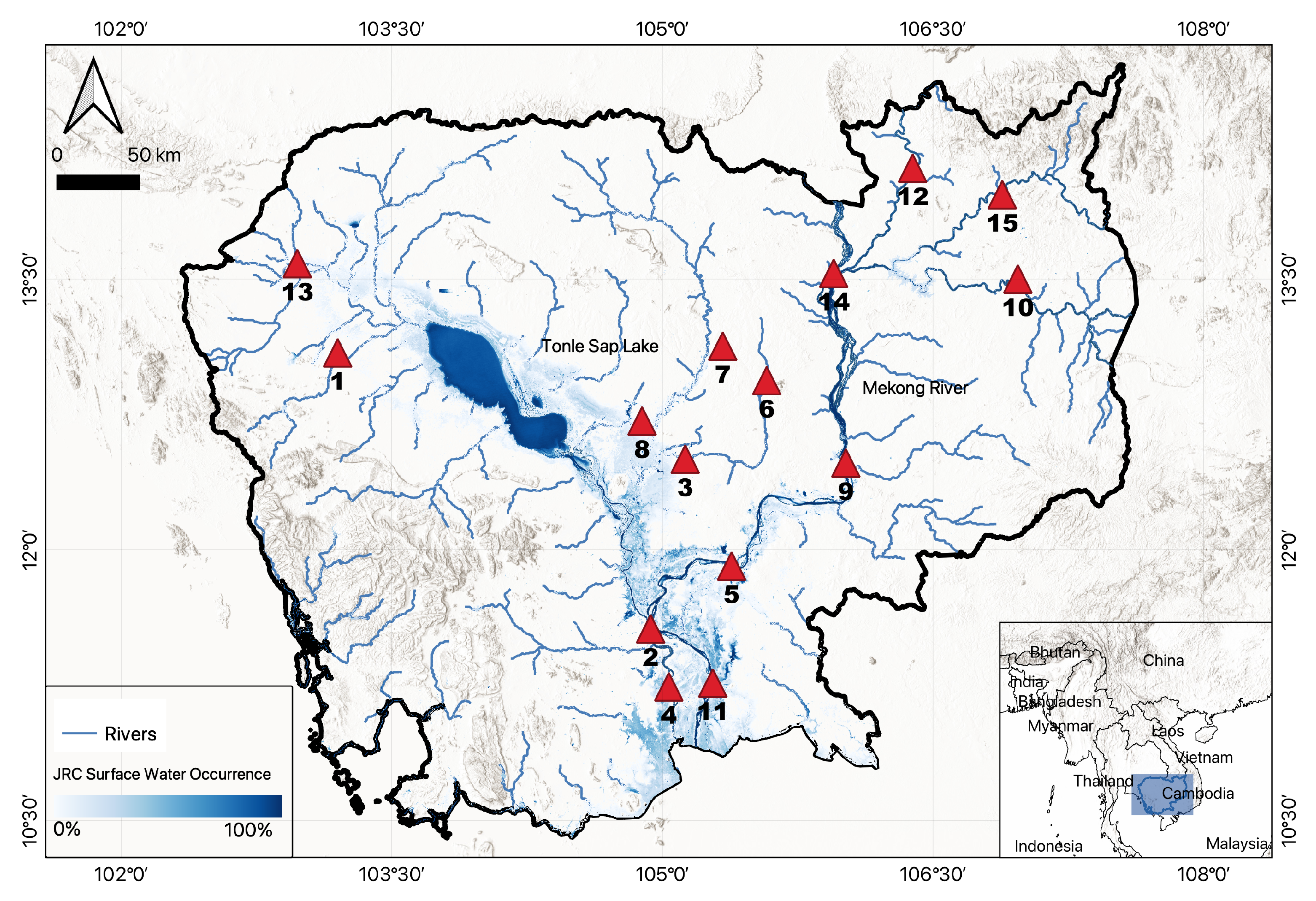
Figure 1 shows the locations of the 15 stations used in this study (red triangle). It also shows the spatial patterns of the Mekong River and Tonle Sap Lake (TSL) (two primary hydrological agents). The Mekong River meets the Mekong Delta of Vietnam on the Southern side. Cambodia contributes about 18% of the discharge annually to the Mekong River Basin (MRB) and covers 20% of the MRB catchment [38]. Near Kratie, three catchments (Se Kong, Se San, and Sre Pok) met together to form the largest sub-component in the Lower Mekong Basin (LMB), contributing about a quarter to the mainstream. Besides the Mekong River, the country’s hydrological system is greatly influenced by the TSL. The seasonal cycle defines the unique flow reversal in the TSL, supporting people’s livelihood via agriculture and providing life to one of the world’s wealthiest and most prosperous freshwater marine ecosystems [39]. By the time the water reaches Phnom Penh near TSL, about 95% of the flow has entered the Mekong. The climate and the annual flow in Cambodia (and the Mekong) are highly influenced by the seasonal tropical monsoon, with about 73% of the discharge between June and November [4,38].
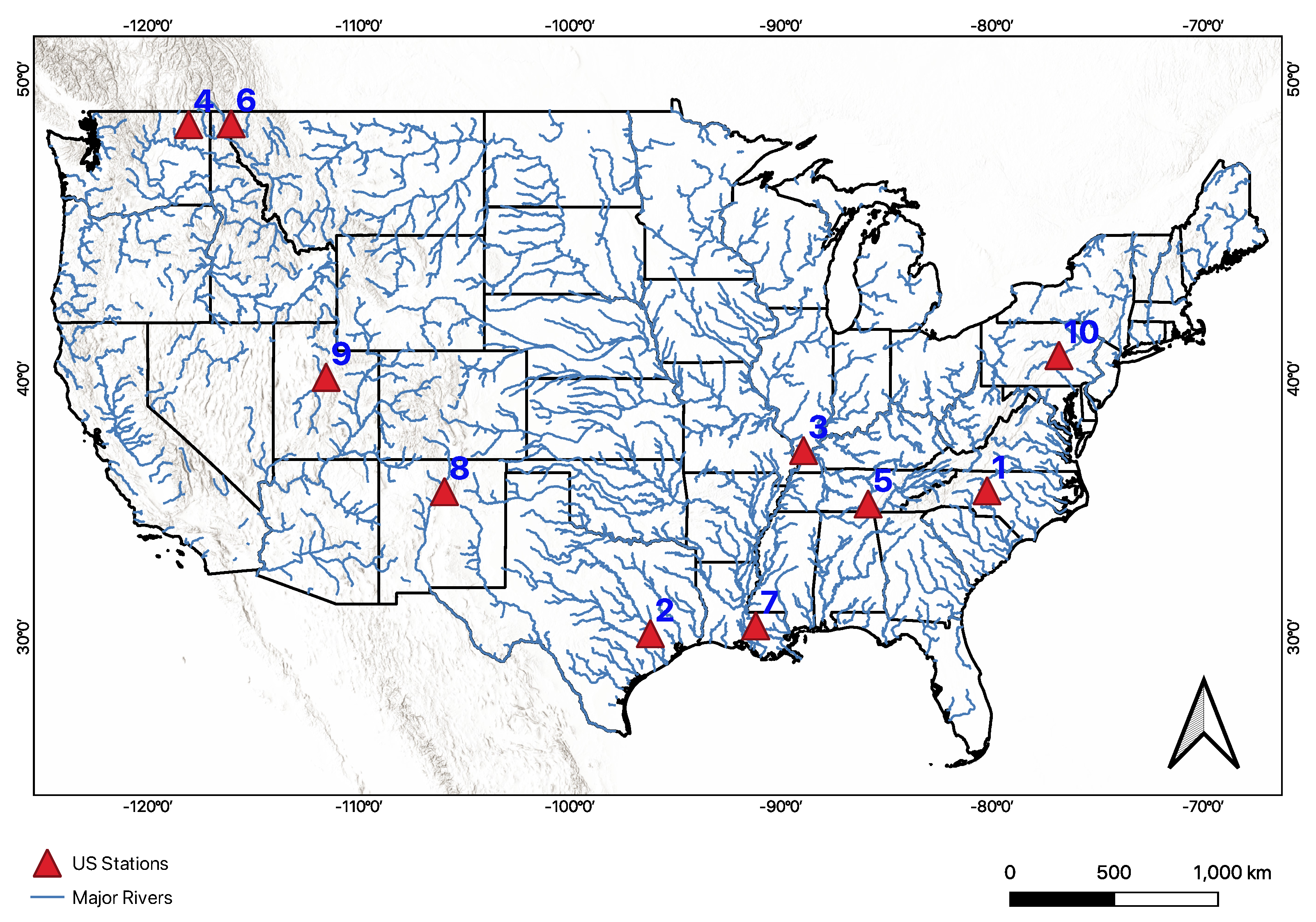
We also applied the methods developed for Cambodia to 10 stations in the US. These stations were selected at random in diverse hydrological region including wet to dry areas representing variations and ranges in streamflow. A random selection of stations was used to prevent sample bias when testing in the US. This was done to test and ensure the method’s robustness, scalability, and transferability and to understand the performance in regions with different hydrological processes. Figure 2 shows the location of ten selected US stations.
2.2. Observation Dataset
We obtained Cambodia’s stream gauge observation data (stage and discharge) from the MRC Data Portal (https://portal.mrcmekong.org/, accessed on 1 April 2022). The MRC gauge stations measure hydrometeorology, climate, and water quality parameters. The selected gauges had both discharge (m/s) and stage height (m) measurements. Some of these discharges were measured as part of the Discharge and Sediment Monitoring Project (DSMP) [40] project. The discharge obtained from DSMP is referred to as measured discharge hereon. Others were provided as the Daily Calculated values; these discharges are referred to as calculated discharge. We did not find any literature on the difference between the calculated discharge and the discharge obtained from the DSMP project. In the case of water level, most gauges make the stage measurement daily. The stage measurement was done manually using gauge reading or automatically by the telemetry reading.
Table 1 lists the selected stations in Cambodia; the ID column corresponds to the station number shown in Figure 1. The ‘Discharge Reported’ column indicates whether the station’s discharge was reported regularly until the study was completed. About 73% of the stations did not report the discharge daily but did report the stage. The RC has not been updated to report the discharge, further signifying the need to update the rating curve. However, Cambodia made several discharge data measurements in the past through the DSMP, which was used in the study.
The stations spread from the Mekong mainstream to the tributaries indicating variations in the watersheds. The available stations had records for an extended period, which is essential in hydrology for understanding the trends and natural (annual/seasonal) cycles [41]. Stung Treng had the longest records that date back to 1910, while Koh Khel records started from 1991.
The measurement data for the US were obtained using USGS API (https://waterservices.usgs.gov/rest/, accessed on 1 June 2022). The discharge was obtained in cubic feet per second (ft/s) and stage in feet (ft) and converted to meters per second (m/s) and meters (m) for consistency. Table 2 lists the stations with their USGS code and location.
2.3. Data Preparation
A total of 15 stations were selected that spread in the Mekong mainstream and tributaries (refer to Figure 1). Both measured and daily calculated data were used in this study. The manual stage and measured discharge observations were given preferences over the telemetry stage or calculated discharge, respectively, in case of duplication. The calculated discharge and telemetry stage data were only used for dates when the measured discharge or manual stage data were unavailable. The measured discharge came from the DSMP project and was measured during the project period, while the calculated discharge was provided as “Daily Calculated” values, with no other information. We did not find any literature on the difference between the daily calculated discharge and the discharge obtained from the DSMP project. The manual stage data was preferred over the telemetry because the manual observation covered the study period more comprehensively and consistently. The telemetry-based stage data may be unavailable due to system failure, maintenance, or other challenges. The common discharge statistics for each stations is shown in Table 3. The datasets were obtained in a daily timescale. This may make it easier for comparison because many global streamflow services, such as Streamflow Prediction Tool (SPT) and Global Flood Awareness System (GloFAS) provide daily forecast values for discharge. However, this also means some of the small basin where the runoff process is fast, those ephemeral events may not be captured well.
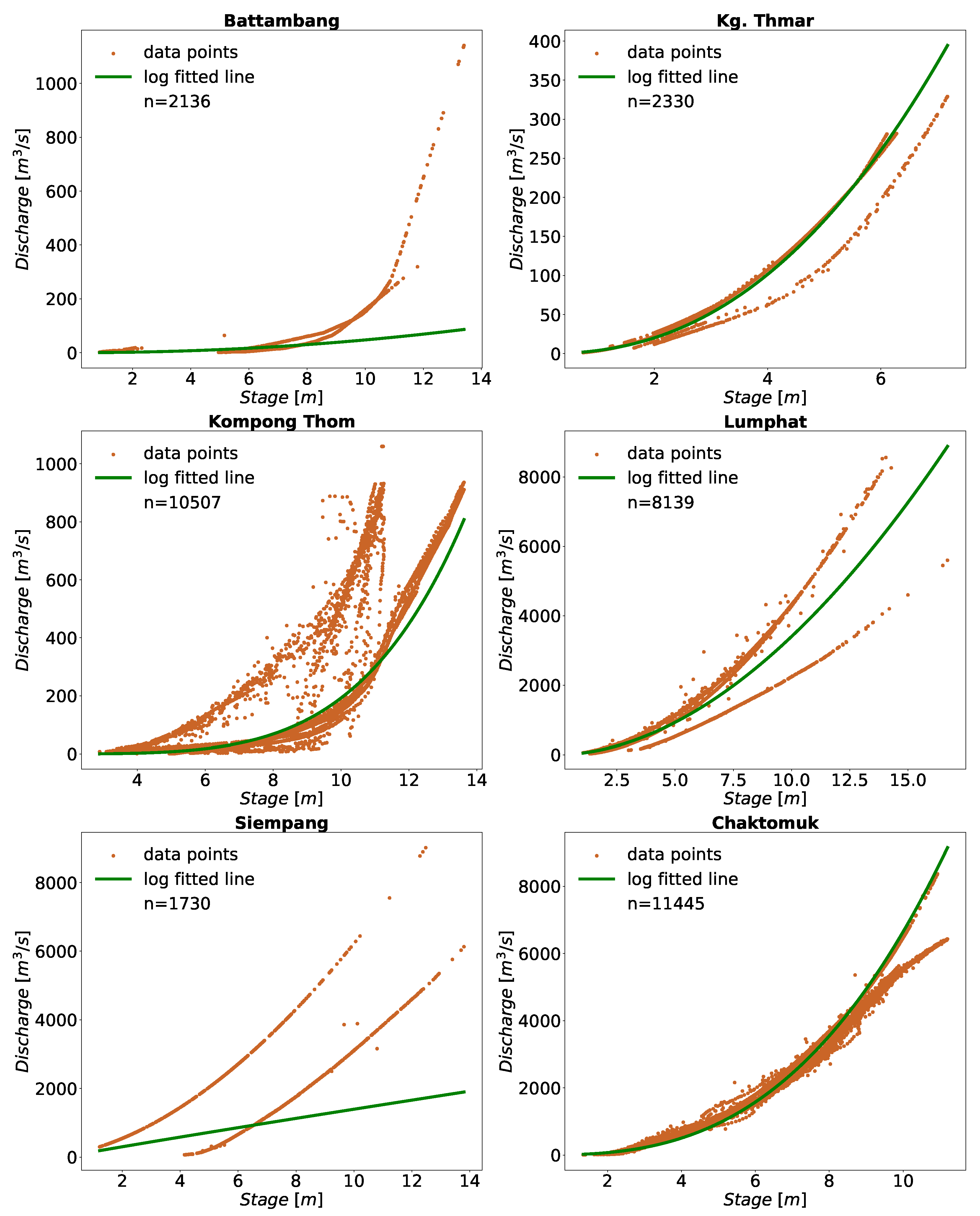
Finally, we fitted the power form (Equation (1)) to the selected station’s data; the result of which are shown in Figure 3 as log fitted line. We noticed that, while some followed the power law, many didn’t fit to the power law. Thus, various preprocessing routines were done before mapping the relation between stage and discharge.
Similarly, the common discharge statistics for each stations in the US is shown in Table 4.
2.4. Methods
Figure 4 shows a high-level Rating Curve generation workflow. A detailed explanation of each step is provided in the following sections. In a high-level, the workflow included filtering the records to a 95% prediction interval, then dividing the data into separate clusters to account for changes in the flood plain before running the outlier detection algorithm in those groups. Finally, a piecewise linear regression was run through the inlier dataset.
2.4.1. Prediction Interval
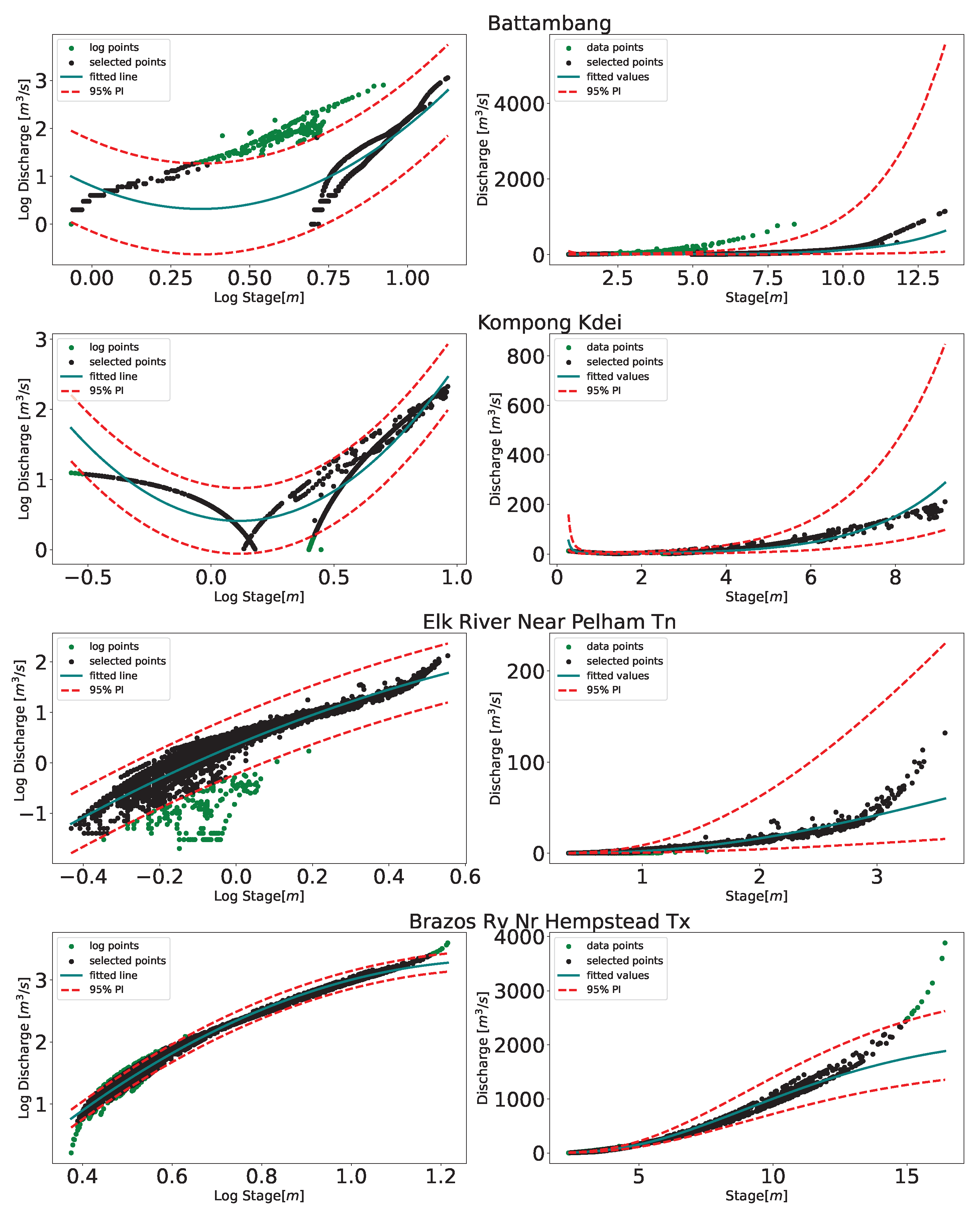
Cambodia’s down-selected stage and discharge data required additional quality control measures to remove erroneous and outlying data values. For quality control, data meeting a 95% prediction interval (PI) were filtered using the second-degree power relation of the stage-discharge.
In most cases, the peak of the data was preserved, while the distribution width (especially in the mid-ranges) was penalized—the implications of the 95% PI in more length are discussed in Section 3. On average, 5% of the data were removed, with a minimum of 0% and a maximum of 8.9% at a given station. The number of data available at each station before and after the 95% PI filtering is shown in the Table A1.
2.4.2. Clustering
Plotting the quality-controlled stage and discharge data revealed that some stations had more than one RC, as shown in Figure 3. As a result, it was necessary to perform additional re-sampling and clustering. Multiple RCs were likely due to significant flood events, noise in the dataset, measurement error, reverse flow (especially near the TSL), or a combination of these factors. For example, severe flooding and flash flooding events were reported during 1996, 2000, 2001, 2010 to 2018 [36] that may have impacted the relation between stage and discharge. In addition, the overland flow of water from the mainstream and the tributaries contributing to TSL can expand up to 14,000 km during the wet season [38,42] and affects Kompong Thom, Kg. Thamar, Kompong Cham, Kratie, and Chaktomuk (where the TSP joins the Mekong River) [43].
The resulting 95% PI data were divided into two clusters obtained via the K-Means clustering algorithm [44]. The K-Means clustering (an unsupervised algorithm) separates the data into K-clusters by minimizing the distance between the cluster center and the data points. The K-Means is an iterative algorithm, so the center of the clusters may change at each iteration [44,45]. Most stations with multiple rating curves showed two clusters (refer to Figure 3); thus, we decided on two groups for the clustering algorithm. The clustering helped to account for changes in the flood plain.
To account for stations that did not need a cluster, we first divided each station’s data into two groups using K-Means. Then, we inspected the Euclidean distance between the center of the clusters. If the distance between the center was less than the specified threshold, we resolved that the station did not need a group. The threshold was determined experimentally, and the length of one unit worked for us. The distance-based approach takes inspiration from the model introduced by [46]. We used both time and stage values as the input clustering features to the K-means, which was valuable in separating the data points at different times in different clusters.
2.4.3. Sampling
Next, the dataset was divided into training and testing using a 3:1 ratio. Finally, the sampling was stratified randomly based on clusters, quantiles, and a mix of clusters and quantiles.
In cluster-based sampling, if the cluster was necessary, each cluster was randomly sampled; else, the entire dataset was randomly sampled. For the quantiles-based selection, the four quantiles (at 25%, 50%, 75% & 100%) were obtained and sampled stratified randomly to get training and testing portions. Then if the cluster was necessary, the training dataset was partitioned into two groupings. For the mixed approach, if the cluster was required, each group was divided into four quantiles. Then, each cluster’s training and testing data were obtained using quantiles as the stratified random sampler. If the cluster was not necessary, we calculated the quantiles of the entire data and got the training and testing data using stratified random sampling.
2.4.4. Outlier Detection
Some stations showed outlier data which could have arisen because of measurement errors or lack of initial quality control. Figure 3 shows some of these stations. Therefore, an outlier detection algorithm was run on each sampled group. We found that, in general, the one-class Support Vector Machine (SVM) [47,48] effectively detected outliers. One-class SVM helps detect outliers in the dataset using kernel function; we used Radial Basis Function (RBF). The RBF kernel forms the envelope around the dataset by transforming the data into a high-dimensional space. This transformation is done in the original feature space without changing the coordinates, commonly called the “kernel trick”. In this study, we did not attempt to quantify the effectiveness or efficiency of outlier detection algorithms; instead, the outlier detection algorithms can be changed as needed. We used the python package sklearn [49] for the outlier detection algorithms. Sklearn supports algorithms related to clustering, outlier detection, and several other ML methods.
2.4.5. Piecewise Curve Fitting
Finally, a linear-piecewise curve was fitted to the obtained inlier data. We experimented with different degree; while keeping scalability, simplicity, and trackability in mind, we decided on two linear curves of second-degree, which provided reasonable accuracy without being overly complicated, to account for high and low flows. Three breakpoints were needed to fit the two linear curves. We used python’s pwlf module [50] to perform the piecewise linear fitting. The starting and ending breakpoints were the minimum and maximum stage values. The second break point was obtained by (1) using the Differential Evolution (DE) [51] and (2) using the 50th percentile of the stage dataset, referred to as percentile break point hereafter. The DE is an iterative optimization algorithm that usually minimizes an objective function [51]; we used the sum of square error. The breakpoint is referred to as auto break point hereafter.
The choice of the breakpoint was made by inspecting the absolute percent difference between them (auto and percentile). We selected the auto break point if the percent difference was within a specific range determined empirically.
2.4.6. Accuracy Assessment
We report three statistical parameters to understand the performance of the model, namely Kling-Gupta Efficiency (KGE) [52,53], Mean Absolute Error (MAE), and Relative Root Mean Squared Error (RRMSE).
KGE is widely used in hydrological applications [54,55]. The KGE provides the decomposition to analyze the three components (correlation, bias, and variability) [52]. The KGE ranges from to 1; the closer to 1, the better the model. Knoben et al. [56] argues that KGE of is equivalent to a model having the same explanatory power as the mean of the observation. The KGE is calculated as
where
where is the bias ratio, is the variability ratio, r is the Pearson correlation coefficient, N is the length of the dataset, is the observed discharge at time t, is the predicted discharge at time t, is the mean of the observed discharge, is the mean of the predicted discharge, is the standard deviation (SD) of the observed discharge, and is the SD of the predicted discharge.
The MAE is the average of the residual for the time series. It provides information on the average quantity that the prediction differs from the observation. The MAE is computed as
where N is the length of the dataset, is the observed discharge at time t, is the predicted discharge at that time, and is the absolute value operator on quantity x.
RMSE is a common measure of performance of model prediction [57]. The RRMSE is a normalized version of RMSE that allows the comparison between different stations at different basins [58]. The RRMSE here is presented in percentage form and calculated as
where N is the length of the dataset, is the observed discharge at time t, and is the predicted discharge at that time, and is the mean of the observed discharges.
3. Results & Discussions
3.1. Application in Cambodia
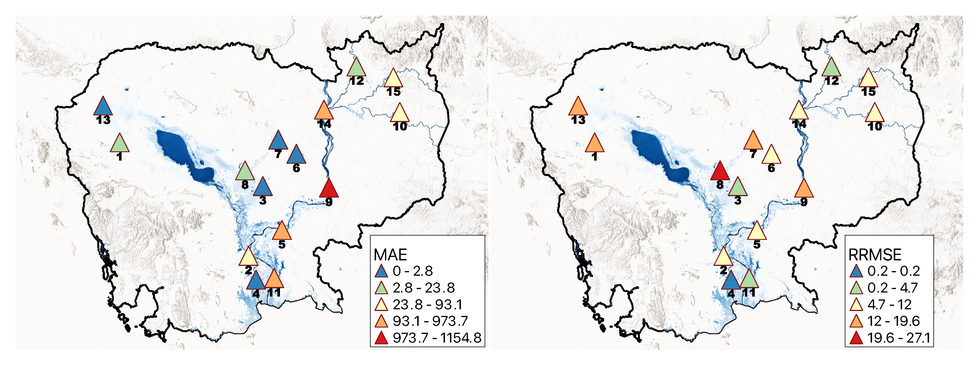
The sampling technique with the mixed approach as described in Section 2.4.3 worked best for Cambodia. The result of validating 25% of the data per station is shown in Table 5. The KGE was >96% for all stations. The MAE ranges from 0.6 to 1154.8 m/s, with around 47% of the stations having a single-digit MAE, and 60% having a single-digit RRMSE. Since the KGE is high (>96%), we have only shown each station’s MAE & RRMSE values in Figure 5. Table 5 also presents the overall mean and standard deviation (SD) for each statistic. The model produced an average KGE, MAE, and RRMSE of 99.1%, 199.8 m/s, and 10.8% respectively, with the average SD of 1%, 369.3 m/s, and 7.6% for KGE, MAE, and RRMSE, respectively. Overall, the stations on the Mekong main river channel (Kompong Cham, Kratie, Neak Luong, and Stung Treng) had lower RRMSE (10.0%) than other stations (11.1%).
Additionally, we determined three levels of flows (high, medium, and low) for each stations. The high flow records were defined as the flows equal or above the 80th percentile flow () for the station; the low flow records were defined as the one equal or below the 20th percentile flow () for the station, and anything in between () was defined to be mid flow records. The MAE and RRMSE were calculated for each flow level from the discharge estimates for each station and shown in Table 6, where the mean and SD for each flow are also shown. The MAE for the mid flow records was almost five and half times (5.4×) more that of the MAE for the low flow records, while the MAE for the high flow records was nearly three times (2.9×) of the mid-flow records. In contrast, the high flow records had the lowest RRMSE which was two and half times (2.5×) lesser than the low flow records. The mid flow records had the highest RRMSE which was more than two and half times (2.8×) than the low flow records.
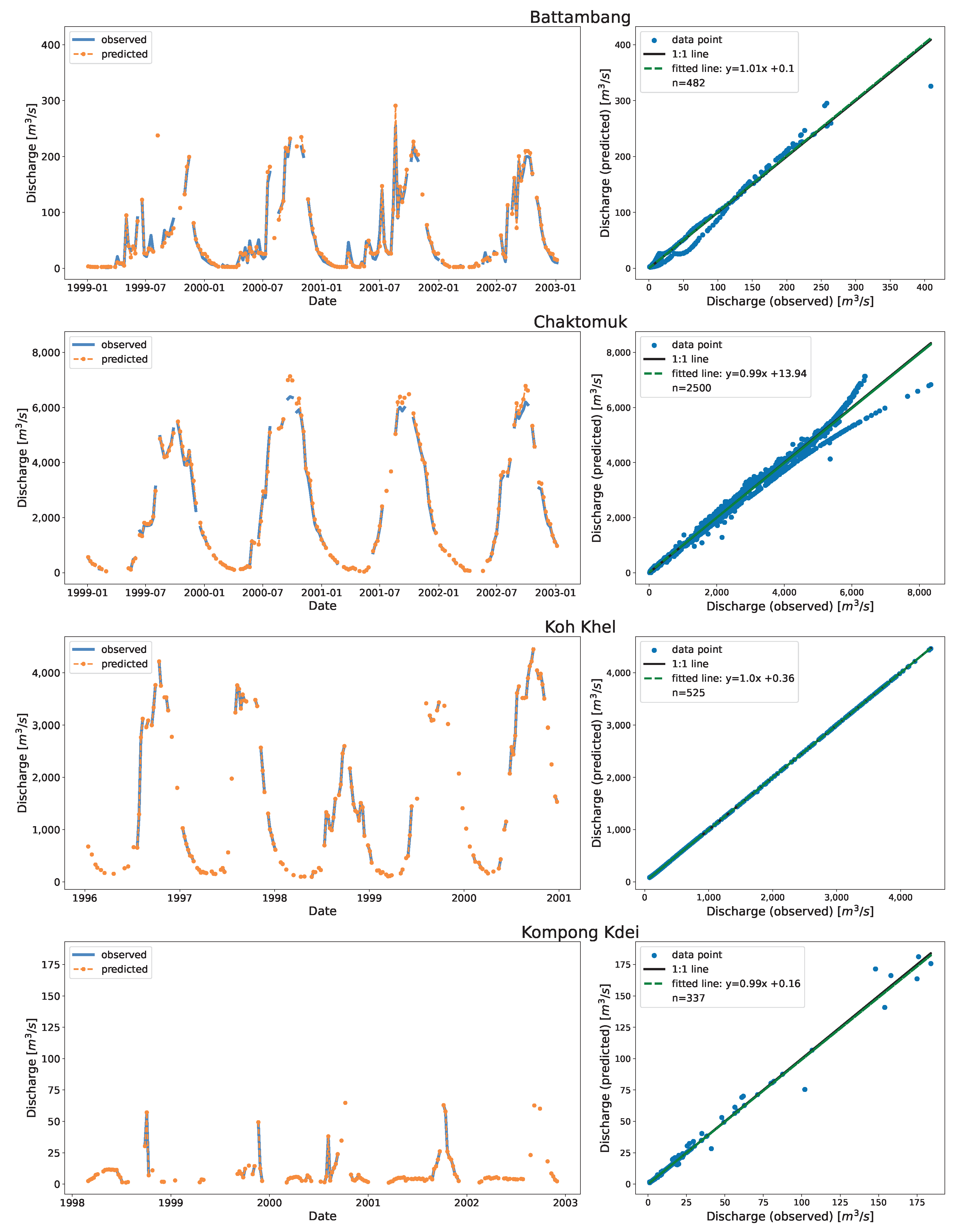
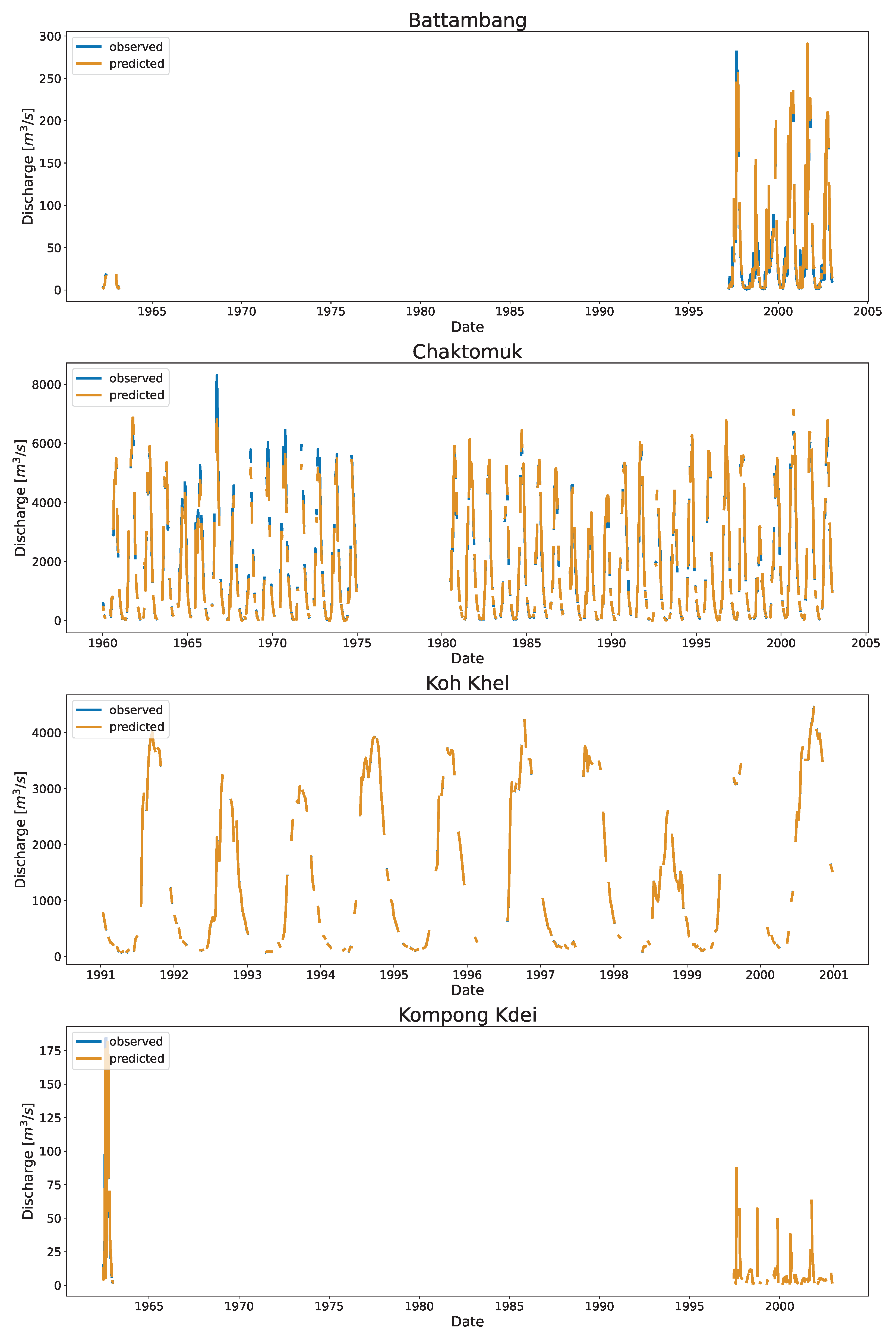
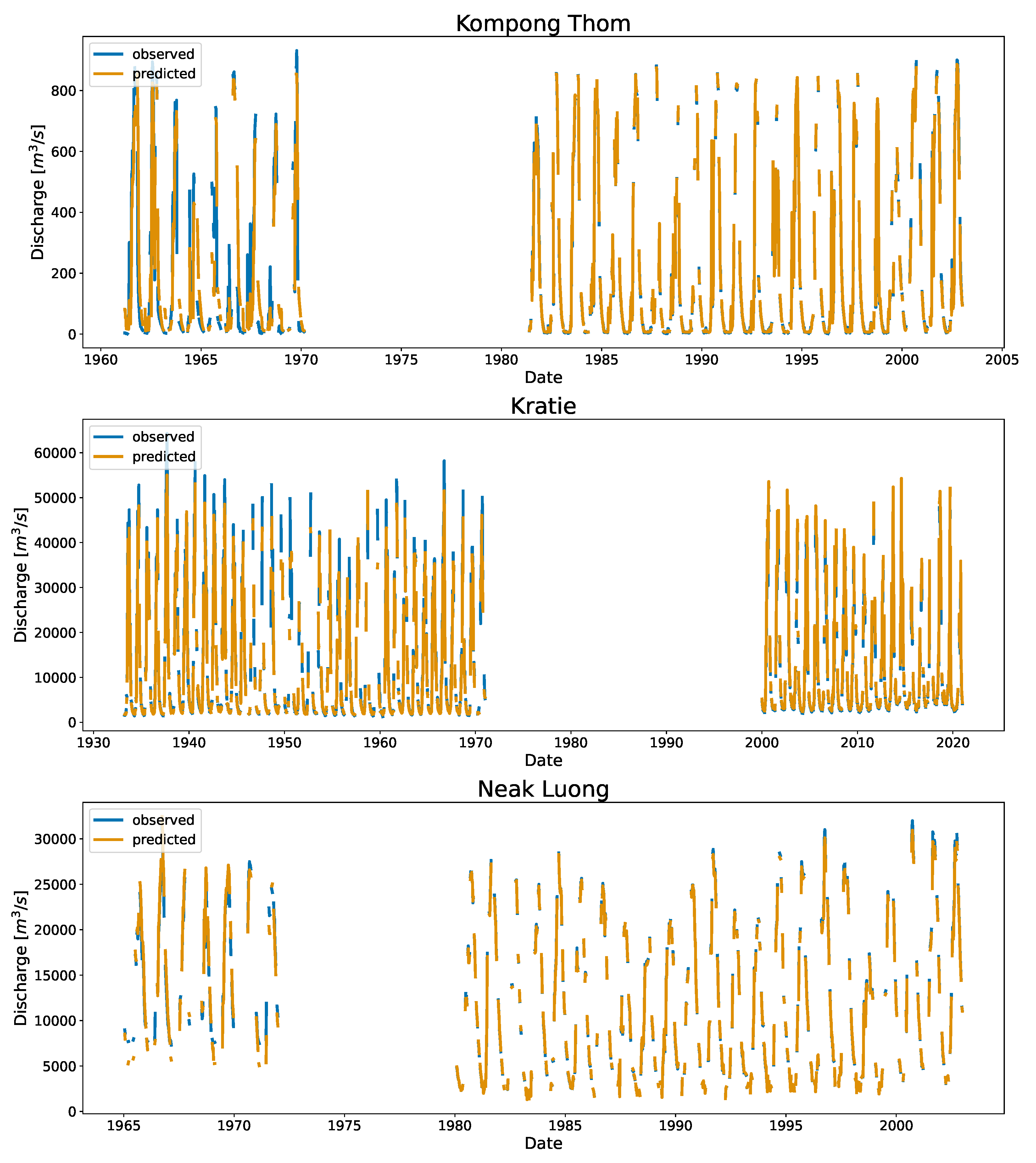
Figure 6 shows the time series and the associated scatter plots of the discharge as estimated using DDRC against observed data for Cambodia. The plot show the 1:1 line to highlight the differences between the simulated and observed streamflow data. The stations shown in Figure 6 have stations affected by the overland flow of the TSL (Chaktomuk & Kompong Thom), and stations with range of discharge (Battambang, Kompong Kdei, Koh Khel, Kratie, & Neak Luong).
The scatter plot at Kompong Thom, which had the highest RRMSE, shows that the prediction was poor at the low end compared to the high end. There is a data gap between the years 1970 and 1982 (Figure A1). The data gap could be due to Cambodia’s political instability because of Civil War [59,60]. Chaktomuk’s data appeared to have split into two ends at the high end. The model approximates the discharge by taking the values between two splits. The model at Neak Luong showed constant under prediction at low end before 1972 (Refer to Figure A1). The base flow of Neak Luong before 1972 has changed from that after 1980, which may be due to the massive flooding that occured in 1978 [61]. The clustering with time and stage as input features captured this variation. The model perfectly fits at Koh Khel (with KGE of 1.0). The station had a well-distributed dataset at low, mid, and high flow records.
3.2. Application in the US
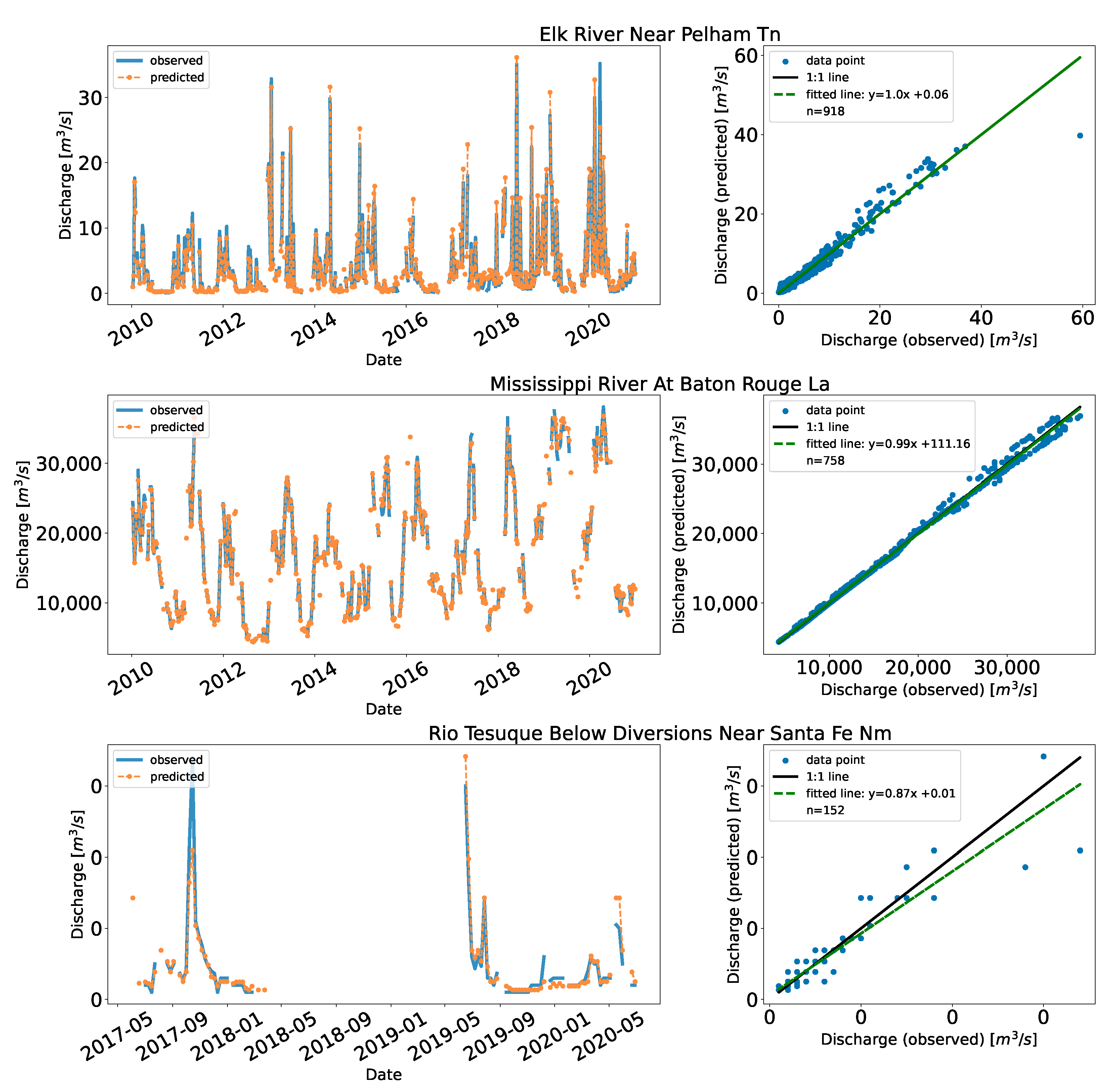
We applied the method to some stations in the US obtained from USGS. These stations were selected in random to represent range of flows. (e.g., Rio Tesuque below diversions near Santa Fe in New Mexico & Mississippi River at Baton Rouge in Louisiana).
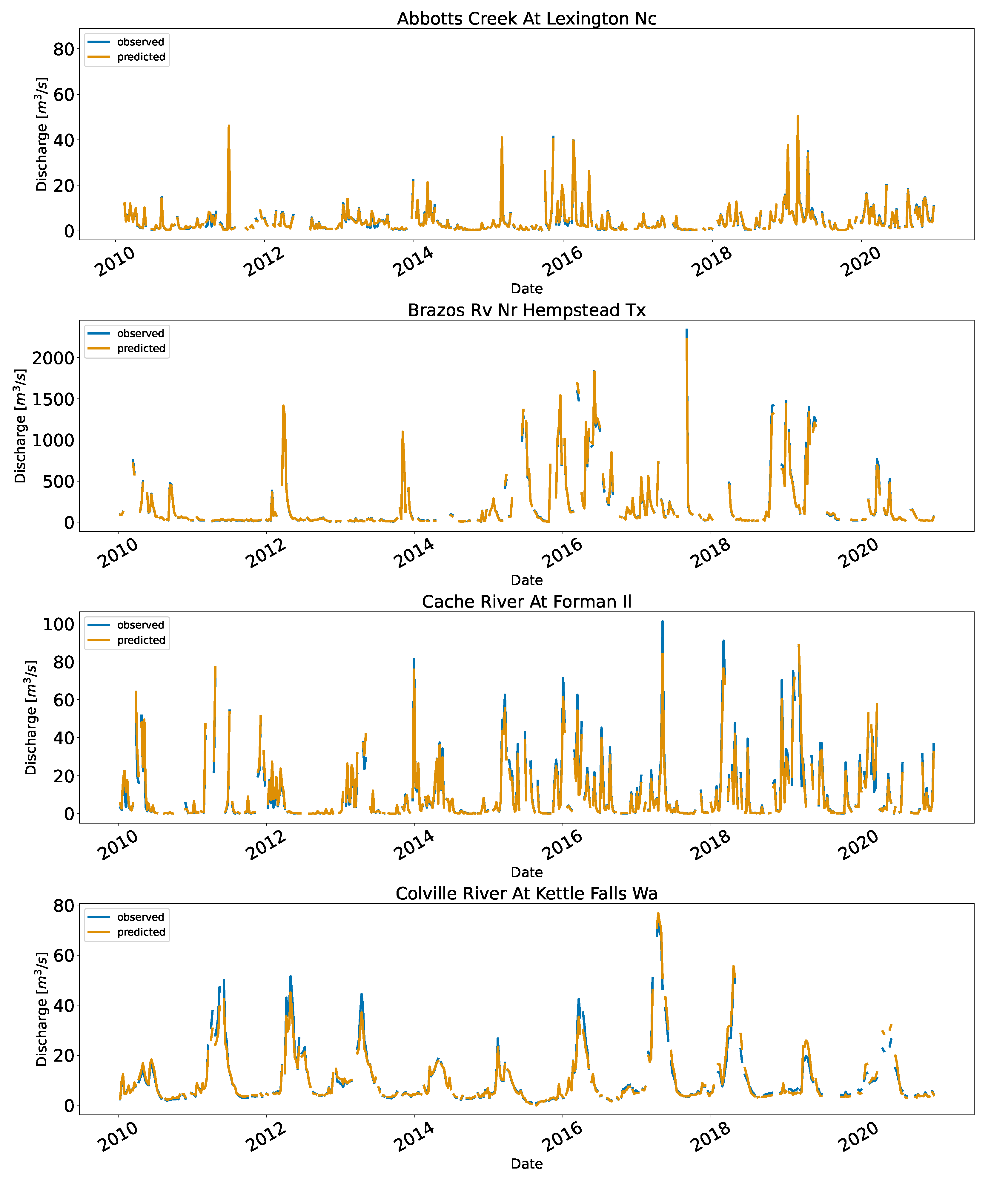
Since USGS performs quality control on the data, we used ten years of data (2010 to 2020). The sampling technique with the mixed approach worked best for the US as well. The results of validating 25% of the data per station are shown in Table 7. The KGE values are similar to Cambodia (>0.90 for all stations); the MAE had a lower range, for example, the Brazos River Near Hempstead (mean flow of 228.2 m/s) had MAE of 10.50 m/s, while a similar flow station in Cambodia, Kompong Thom (mean flow of 235.2 m/s) had MAE of 23.83 m/s. This could be because of the overland flow of water at Kompong Thom as discuss more later. A high-flow station in the US placed at the Mississippi river at Baton Rouge had lower MAE of 296.22 m/s; the high flow station in Cambodia, Neak Luong which had MAE of 351.57 m/s. This may be because of data quality especially the dataset before 1973 for Neak Luong. Figure 7 shows the time series and the scatter plots for the implementation in the US.
Similar to Cambodia, we determined three levels of flows (high, medium, and low) for each stations with the same definition, where the high flow records were the flows equal or above the 80th percentile flow () for the station, the low flow records were the one equal or below the 20th percentile flow () for the station, and anything in between () was defined to be mid flow records. The MAE and RRMSE of this analysis for each station is shown in Table 8. The MAE for the mid flow records was almost twice (1.7×) that of the MAE for the low flow records, while the MAE for the high flow records were four times (4.0×) the mid flow records. In contrast, the high flow records had the lowest RRMSE which was almost one and half times (1.3×) lesser than the low flow records. The mid flow records had the highest RRMSE which was almost two and half times (2.4×) more than the low flow records.
3.3. Discussion
The analysis of results from both Cambodia and US stations suggest that the proposed method worked well across the regions. We used time-series information to understand the changes in the floodplain to generalize the RC. The method is scalable, automatic, and modular; choices for different routines in the methods can be switched, added, or removed.
Results showed that the high flow records had lower errors associated with them (Table 3 and Table 4) and was observed in both cases of the Cambodia and the US status. The practical implications for these results comparing high, mid, and low flow show that the DDRC method is better at predicting discharge from gauge height during high flow events (i.e., flood events). Conversely, during low flow events (i.e., Drought periods) the estimated discharge is shown to have a lower accuracy. This was also consistent with study by [62] who used Gene Expression Programming (GEP) [63] as a data-derived approach, and found that GEP was more reliable for extreme flood events.
Similarly, the distribution of the data points affected the performance. The Rio Tesuque station near Santa Fe in New Mexico had lower KGE (90.9%) and highest RRMSE (39.1%) than other stations. The fitted model was under predicting which is evident by the slope of the fitted line (0.87) which was less than 1.0. This is an extremely low flow station ( = 0.04 m/s), with few data points and gaps between 2018 and 2019. The data points are concentrated at the lower end compared to the mid and high end. Likewise, Elk River near Pelham in Tennessee had few points on the high end. We observed underpredictions during the early years (2010–2013). In Mekong, main stream stations–Kompong Cham, Kratie, Neak Luong, and Stung Treng had almost 62% of the record (refer to Table A1), and thus probability of capturing high and low end is better. The stations in the mainstream were found to have relatively lower RRMSE (average of 10.0% across the mainstream stations vs. 11.1% for the rest) despite having higher MAE (average of 695.0 m/s across the mainstream stations vs. 19.7 m/s for the rest). The higher MAE in the mainstream is because of their large flow (average of 13,399.5 m/s vs. 632.5 m/s for the rest), seasonal variations in discharge, and reversal flow of the TSL.
The effect of reversal flow between TSL and Mekong can be seen in the nearby stations. For example, Kompong Thom, on the tributary, suffers from the overland flow from the TSL and the Mekong river [64]; thus Kompong Thom has the highest RRMSE. The high flow records were better captured than the mid and low flows (Refer to Table 6). A similar effect can also be seen in mainstream station Kompong Cham and Kratie which are affected by the overland flow between TSL and Mekong River. Kratie is generally considered to be the starting point for the reverse flow [4]. The MAE for Kratie and Kompong Cham (1154.82 m/s and 973.74 m/s, respectively) are worse than other mainstream stations—Neak Luong and Stung Treng (351.57 m/s and 299.95 m/s, respectively). The TSL meet the Mekong river at the confluence of the Chaktomuk, greatly influencing this station’s high and mid flow (Refer to Figure A1). Below this, the river splits into Bassac river and the Mekong river.
Other stations in Mekong, Battambang, and Sisophon also had high RRMSE with few data points on the high end. These stations lie on the tributaries outside the Mekong mainstream and contribute downstream to the Tonle Sap Lake. Seasonal rainfall may be linked to the increased flow during the wet season (Refer to Figure A3) with a very low baseflow during the dry season. The other reason could be that those points were outliers not detected by the outlier algorithm. Similarly, stations in the US also have seasonal spike in their flow due to the rainfall events (Refer to Figure A4)
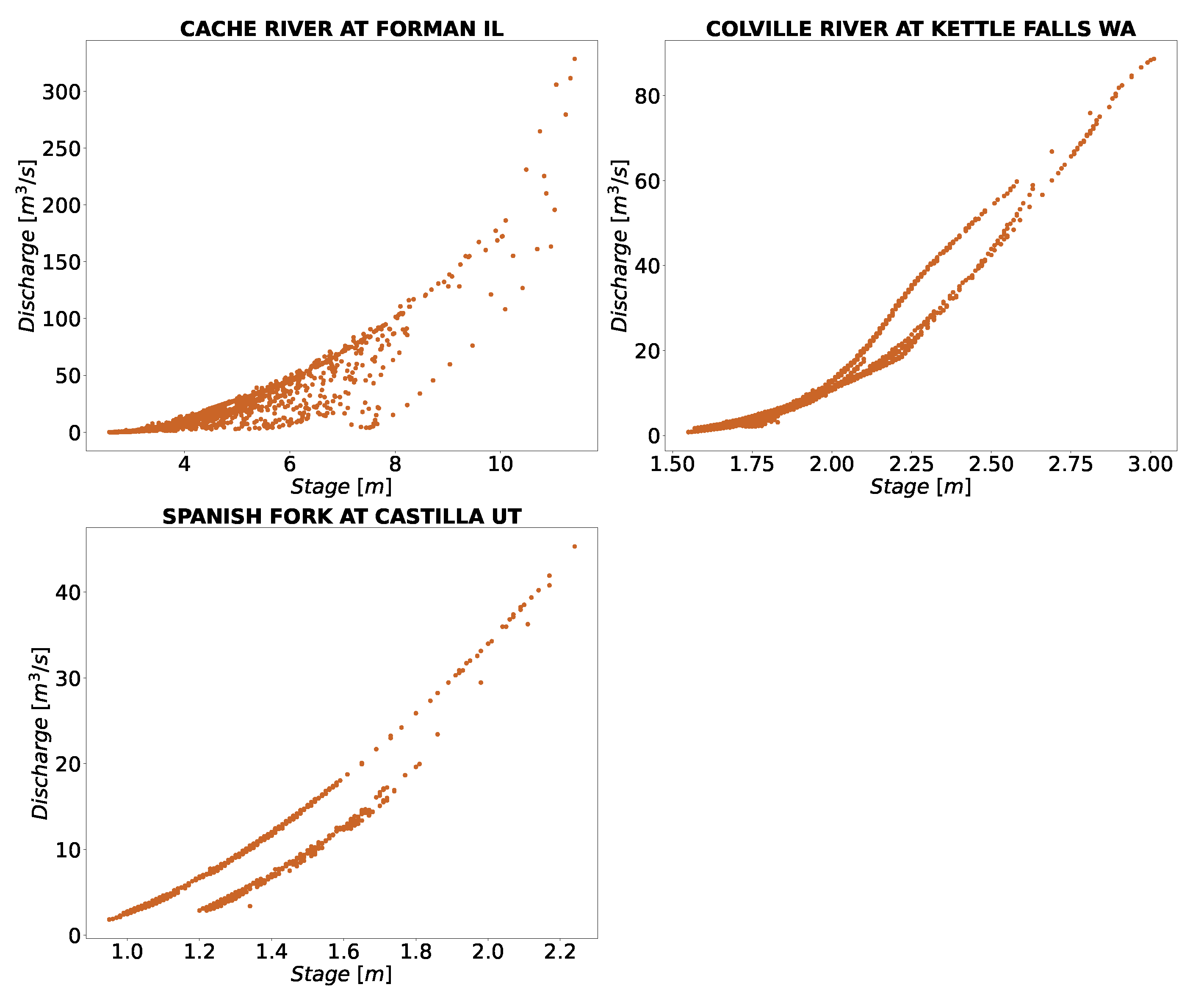
The rating curve tends to change over time; we noticed this phenomenon in several stations. The stations shown in Figure 3 represent such conditions at stations in Cambodia, where different rating curve was observed. Some of the changes for the stations in the US are shown in Figure 8. The runoff generating in Cambodia has a strong seasonality related to the wet season (June to November). Thus, separate rating curve may be explained by the rising and falling stage hydrograph. For stations considered here, depending upon dry or wet year, there could be up to two to three peaks with clear seasonality [4,65]. These are usually prevalent for high flow stations, like Stung Treng and Kratie. Thus, the clustering technique with the piecewise regression attempts to separate those rating curve and capture the non-linearity of the hydrograph.
One of the major opportunities (and a challenge) for the method was data quality in Cambodia. Significant data gaps or incomplete records were observed in many stations; in Neak Luong, the low flow was significantly different before 1971 compared to after the 1980s, with a data gap in between. Similarly, we observed that the model was mostly under predicting before the gap years (around 1970 or 1975) in Chaktomuk, Kompong Thom, and Kratie (Figure A1). This may be linked to data quality or the inadequacy of the K-Means to separate them; other clustering algorithms based on density for example Density-Based Spatial Clustering of Applications with Noise DBSCAN [66,67] or based on distribution for example Gaussian Mixture Model [68] may perform better.
We considered a second-order power stage-discharge relationship as this was found experimentally to fit most stations without being overly complicated in Cambodia. This relationship was consistent with the result [69] found in their study in the Mekong using the satellite altimetry stage data. With this relation, we then performed a 95% prediction interval. We noticed that, while this removed outliers from most of the stations and performed well, for some stations, e.g., Brazos River near Hempstead in Texas, as shown in Figure 9, a higher-order relation may be desirable. In another study [19], this station near Hempstead in Texas was also used. Even with the second-order relation removing some points in the high end (refer to Figure 9), the maximum discharge was set at 2432.41 m/s in this study as opposed to 1605 m/s in [19]; the NSE [70] and RMSE of validation data-points (calculations not shown here) were 0.996 and 21.4 m/s while it was 0.941 and 34.31 m/s in [19]. Thus, the longer time series gives higher probability of capturing the high-end or low-end events, which may be considered as a built-in extrapolation characteristics as compared to a traditional method where few data points are often used.
We tweaked several parameters that affected the model’s performance. These were determined experimentally. Some of them are:
- (1)
- Threshold, controlling the absolute percent difference between the auto and percentile breakpoint, took numerical values.
- (2)
- The Euclidean distance between the centers of the clusters: this parameter determined whether the cluster was necessary for the station and took numerical values.
- (3)
- The outlier detection contained various parameters in the algorithm. For example, sklearn’s OneClassSVM, which was used in the study, has parameters like the upper bound on the fraction of training error (also called nu), choice of kernel, and kernel coefficient.
We determined a single set of parameters for the country. Adjusting individual station parameters may be desirable during an operational implementation of the method, which may further increase the confidence in the rating curve. Furthermore, we constrained our rating curve model to second-order polynomial fitting which may not represent the dynamics of the gauge height and discharge relationship in all cases. Additional constraints include assuming only one to two clusters for gauge height-discharge relationship where some stations may have three or more clusters. The rating curve results are only relevant within the data range of the training data used, extrapolating the rating curve outside the data range could lead to several uncertainties [23,71]. We did not test the error uncertainty for extrapolation, which should be used cautiously, although a time series based rating curve has higher probability of capturing the high-end and low-end events, as explained above, compared to traditional method where lesser data points are used. This study did not inspect the threshold for number of data points required to produce accuracy results (for the final results and at each step in the workflow), although investigation of how limited data influence the data driven results will be explored in future work. For this study the fewest number of data points to create the rating curve was 152 points at the Rio Tesuque Diversions station (Figure 7). From a practical point of view, this method is useful for converting gauge height measurements to discharge, where there is relatively limited discharge data that is not measured regularly has not been updated.
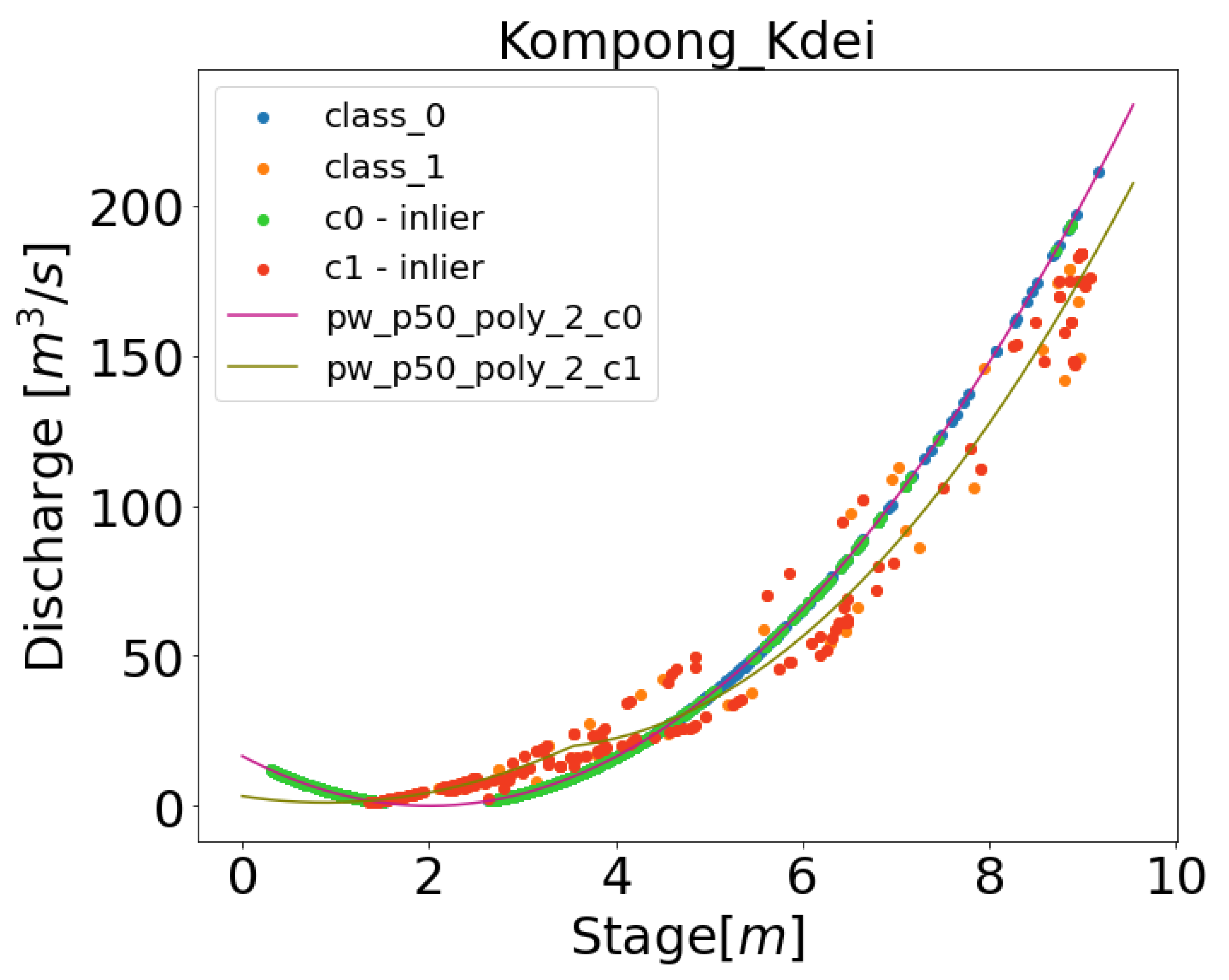
Data driven approaches typically obscure the decisions being made on data to produce the results [72]. Model interprebility for data driven approaches is important within the scientific disciplines as it lends to understanding of the models decisions and supports scientific discovery. The methodology presented in the paper combines multiple interpretable models including K-Means clustering, one-class SVM, and piece-wise polynomial regressions. As such, the different data driven decisions can be inspected and interrogated for additional information. Figure 10 displays the results from multiple steps of training the DDRC for a station, in this case Kompong Kdei. It can be seen that the clustering determines the two best rating curves, while the outlier detection removes certain data points to refine a rating curve. Each individual component of these models can be output and interpreted to better understand how the data has informed the final rating curve result. Additional knowledge on particular flooding event to determine the breakpoints maybe integrated to increase the fitting accuracy of the rating curve. In addition to including physical attributes to drive the rating curve fitting, Physics Informed Neural Network (PINN) can be implemented in order to increase the robustness and interpretability of the model, for example, to incorporate information on backwater may also benefit. Future work will include investigating the application of PINNs for the rating curve fitting process.
4. Conclusions
We introduced a data-driven method for automatically generating the stage-discharge rating curve and showed uncertainties using a statistical approach. The technique utilizes time-series information to understand the changes in the floodplain to generalize the rating curve. The method is modular; choices for different components can be switched, added, or removed. To ensure the robustness and generalizability of the process, we applied the method to fifteen stations in Cambodia and ten stations in the US; we found comparable results. In Cambodia, we obtained overall Kling Gupta Efficiency (KGE) of 99% & an average Relative Root Mean Squared Error (RRMSE) of 12% with an average Mean Absolute Error (MAE) of 200 m/s. In the US, overall KGE was 97%, with an average RRMSE of 17% and an average MAE of 32 m/s. In many stations, we noticed the change in the rating curve over time, confirming the general phenomenon in hydrology. We found that the method had lower RRMSE at high flow records compared to mid and low flow records, despite having higher MAE because of large flow and seasonal variations in discharge. The distribution of the data points also affected the performance. Similarly, the effect of precipitation and the reversal flow between Tonle Sap Lake (TSP) and the Mekong River was discussed. We also found that the time series approach has higher probability in capturing the high-end and low-end events compared to the traditional method, which usually use few data points and can be considered a built-in extrapolation feature in the time series approach. We generalized the parameters across the country; however, the accuracy can be further increased if the parameters were tweaked per station basis. In addition, we discussed some of the limitations of the method and provided suggestions on taking the research to operational mode and improving the model’s accuracy. In a nutshell, the time series-based process has valuable information to update the rating curve, especially in a data-scarce environment.
Author Contributions
Conceptualization, B.B., K.M. and A.M.; methodology, B.B. and K.M.; software, B.B.; validation, B.B.; formal analysis, B.B.; resources, B.B.; data curation, B.B.; writing—original draft preparation, B.B.; writing—review and editing, B.B., V.M., A.M. and R.G; visualization, B.B.; supervision, R.G. All authors have read and agreed to the published version of the manuscript.
Funding
This research was funded by the joint US Agency for International Development (USAID) and National Aeronautics and Space Administration (NASA) initiative SERVIR under the NASA Cooperative Agreement: 80MSFC22M001.
Institutional Review Board Statement
Not applicable.
Informed Consent Statement
Not applicable.
Data Availability Statement
The observed stage discharge data for Cambodia and US were obtained from https://portal.mrcmekong.org/, accessed on 1 April 2022 and https://waterservices.usgs.gov/rest/, accessed on 1 June 2022, respectively. The Jupyter Notebook developed to generate the rating curve is open-source and can be found on GitHub https://github.com/biplovbhandari/ddrc-repo accessed on 1 June 2022.
Acknowledgments
The authors would like to acknowledge the Mekong River Commission (MRC) for allowing us to use their data for research purpose, Sundar Christopher for their guidance throughout the project, and Lee Ellenburg for their comments on the manuscript. Finally, we extend our appreciation to the reviewers for their comments that ultimately improved the quality of the manuscript.
Conflicts of Interest
The authors declare that they have no known competing financial interests or personal relationships that could have appeared to influence the work reported in this paper.
Appendix A. Result of 95% Prediction Intervals

Table A1.
The table presents the number of records before and after applying the 95% PI to the station records. On average, 5.0% of the data were removed.
Table A1.
The table presents the number of records before and after applying the 95% PI to the station records. On average, 5.0% of the data were removed.
| Station | # Points Before PI | # Points After PI | % Change |
|---|---|---|---|
| Battambang | 2344 | 2136 | 8.9 |
| Chaktomuk | 11,941 | 11,445 | 4.2 |
| Kg. Thmar | 2462 | 2330 | 5.4 |
| Koh Khel | 3653 | 3626 | 0.7 |
| Kompong Cham | 15706 | 15331 | 2.4 |
| Kompong Chen | 1807 | 1693 | 6.3 |
| Kompong Kdei | 1592 | 1487 | 6.6 |
| Kompong Thom | 11,302 | 10,507 | 7.0 |
| Kratie | 21,331 | 20,112 | 5.7 |
| Lumphat | 8679 | 8139 | 6.2 |
| Neak Luong | 10,449 | 9850 | 5.7 |
| Siempang | 1730 | 1730 | 0.0 |
| Sisophon | 1384 | 1311 | 5.3 |
| Stung Treng | 40,543 | 39,114 | 3.5 |
| Voeun Sai | 8375 | 7722 | 7.8 |
| Average Change (%) | 5.0 | ||
Appendix B. Full Time Series Plot of Cambodia
Figure A1.
Predicted and observed discharge for Cambodia. For visualization purposes, the data are downsampled into a weekly bin, and the mean values of the discharge failing into the bins for the station are shown.
Figure A1.
Predicted and observed discharge for Cambodia. For visualization purposes, the data are downsampled into a weekly bin, and the mean values of the discharge failing into the bins for the station are shown.


Appendix C. Full Time Series Plot of the US
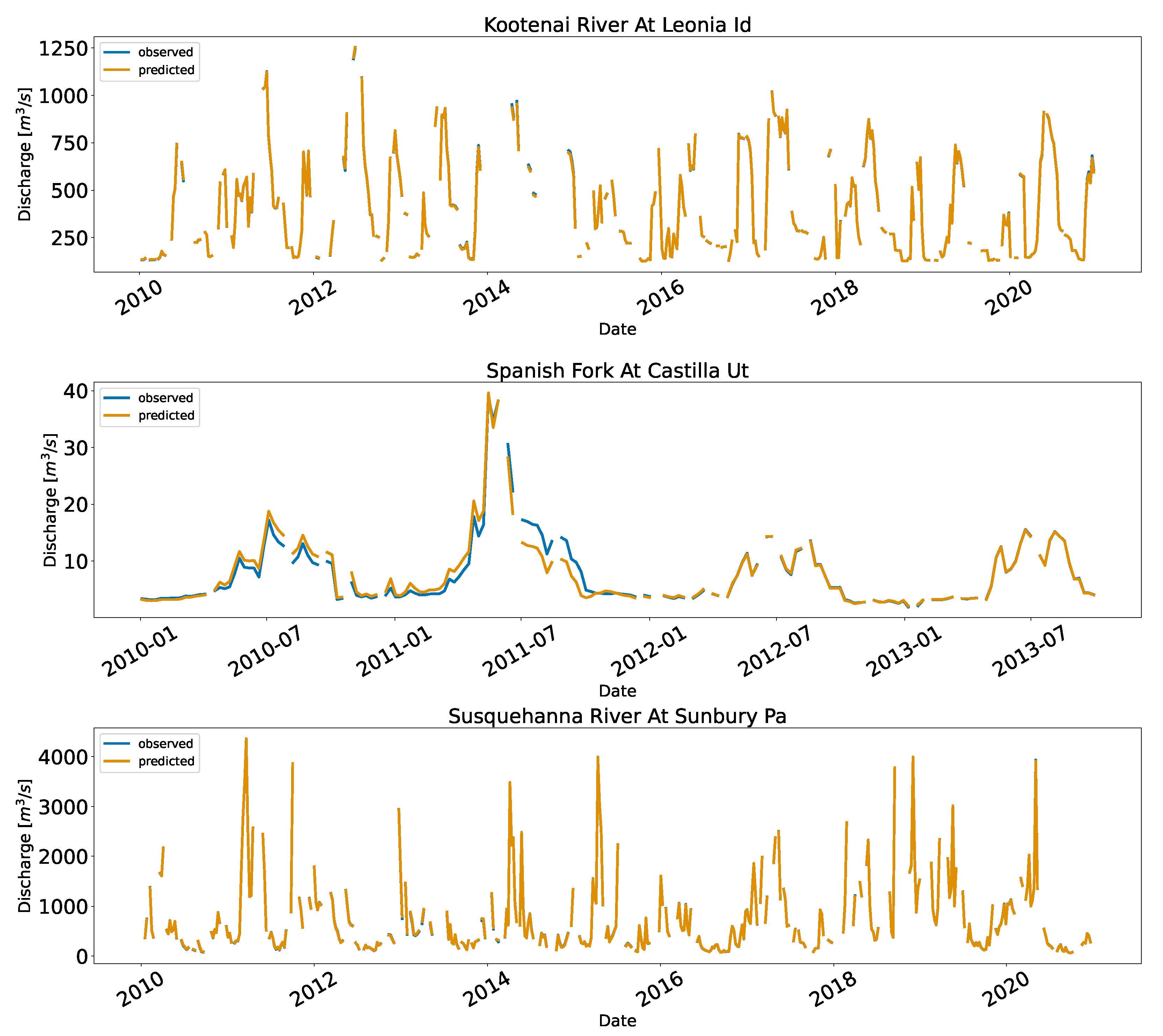
Figure A2.
Predicted and observed discharge for the US. For visualization purposes, the data are downsampled into a weekly bin, and the mean values of the discharge failing into the bins for the station are shown.
Figure A2.
Predicted and observed discharge for the US. For visualization purposes, the data are downsampled into a weekly bin, and the mean values of the discharge failing into the bins for the station are shown.


Appendix D. Plot of Precipitation and Discharge
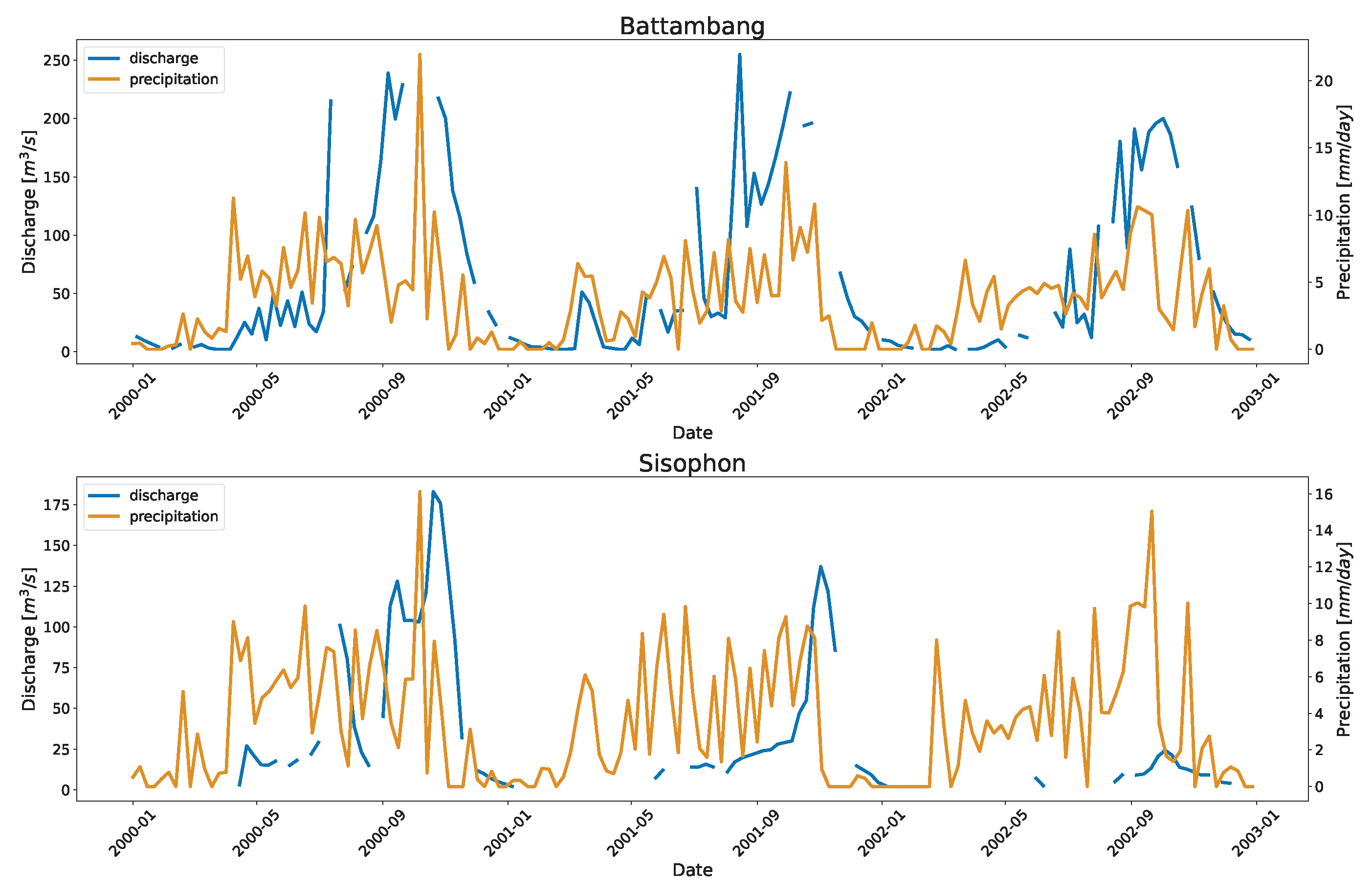
Figure A3.
Plot of precipitation taken from CHIRPS [73] and the observed discharge. For visualization purposes, the data are downsampled into a weekly bin, and the mean values are shown. The left y-axis is for discharge (blue plot), and the right y-axis is for precipitation (orange plot).
Figure A3.
Plot of precipitation taken from CHIRPS [73] and the observed discharge. For visualization purposes, the data are downsampled into a weekly bin, and the mean values are shown. The left y-axis is for discharge (blue plot), and the right y-axis is for precipitation (orange plot).

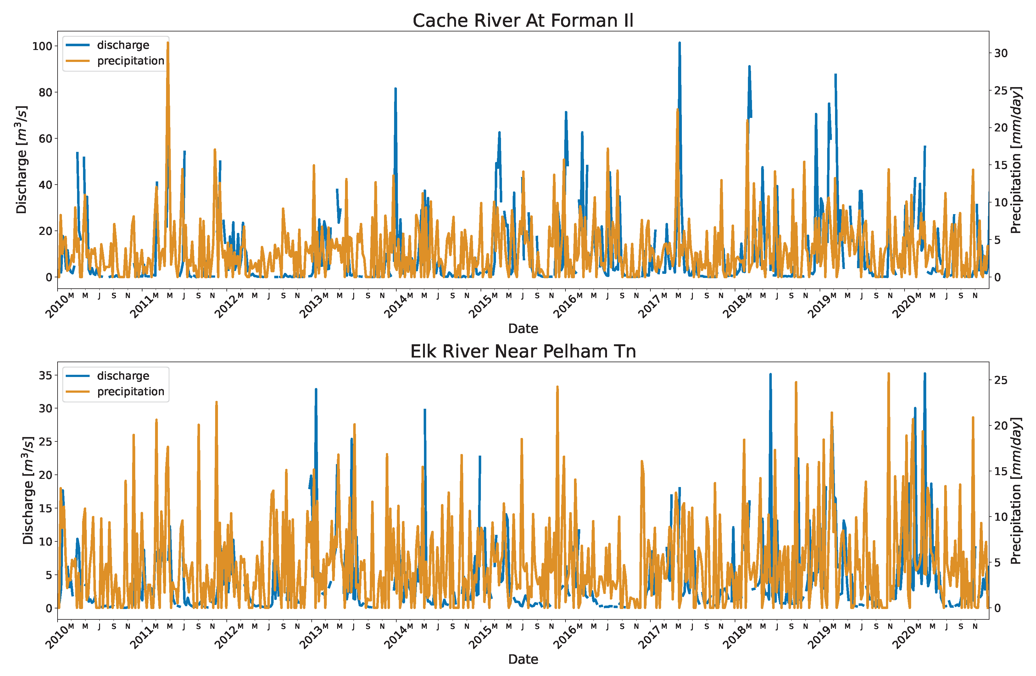
Figure A4.
Plot of precipitation taken from CHIRPS [73] and the observed discharge. For visualization purposes, the data are downsampled into a weekly bin, and the mean values are shown. The left y-axis is for discharge (blue plot), and the right y-axis is for precipitation (orange plot).
Figure A4.
Plot of precipitation taken from CHIRPS [73] and the observed discharge. For visualization purposes, the data are downsampled into a weekly bin, and the mean values are shown. The left y-axis is for discharge (blue plot), and the right y-axis is for precipitation (orange plot).

References
- Tellman, B.; Sullivan, J.A.; Kuhn, C.; Kettner, A.J.; Doyle, C.S.; Brakenridge, G.R.; Erickson, T.A.; Slayback, D.A. Satellite imaging reveals increased proportion of population exposed to floods. Nature 2021, 596, 80–86. [Google Scholar] [CrossRef]
- Tospornsampan, J.; Malone, T.; Katry, P.; Pengel, B.; An, P.H. Short and Medium-term Flood Forecasting at the Regional Flood Management and Mitigation Centre. In Integrated Flood Risk Management in the Mekong River Basin Proceedings; Mekong River Commission: Bangkok, Thailand, 2009; pp. 155–164. [Google Scholar]
- Werner, M.; Schellekens, J.; Gijsbers, P.; van Dijk, M.; van den Akker, O.; Heynert, K. The Delft-FEWS flow forecasting system. Environ. Model. Softw. 2013, 40, 65–77. [Google Scholar] [CrossRef]
- Pagano, T.C. Evaluation of Mekong River commission operational flood forecasts, 2000–2012. Hydrol. Earth Syst. Sci. 2014, 18, 2645–2656. [Google Scholar] [CrossRef]
- WMO. First Steering Committee Meeting (SCM 1) on the Mekong River Commission Flash Flood Guidance (MRCFFG) System; Technical Report; World Meteorological Organization (WMO): Pnom Penh, Cambodia, 2017. [Google Scholar]
- Azad, W.H.; Hassan, M.H.; Ghazali, N.H.; Weisgerber, A.; Ahmad, F. National Flood Forecasting and Warning System of Malaysia: An Overview. In Water Resources Development and Management; Springer: Singapore, 2020; pp. 264–273. [Google Scholar] [CrossRef]
- WMO. Coastal Flooding Forecast Strengthened in Indonesia; World Meteorological Organization: Geneva, Switzerland, 2019; Available online: https://public.wmo.int/en/media/news/coastal-flooding-forecast-strengthened-indonesia (accessed on 8 February 2019).
- Snow, A.D.; Christensen, S.D.; Swain, N.R.; Nelson, E.J.; Ames, D.P.; Jones, N.L.; Ding, D.; Noman, N.S.; David, C.H.; Pappenberger, F.; et al. A High-Resolution National-Scale Hydrologic Forecast System from a Global Ensemble Land Surface Model. JAWRA J. Am. Water Resour. Assoc. 2016, 52, 950–964. [Google Scholar] [CrossRef] [PubMed]
- Qiao, X.; Nelson, E.J.; Ames, D.P.; Li, Z.; David, C.H.; Williams, G.P.; Roberts, W.; Sánchez Lozano, J.L.; Edwards, C.; Souffront, M.; et al. A systems approach to routing global gridded runoff through local high-resolution stream networks for flood early warning systems. Environ. Model. Softw. 2019, 120, 104501. [Google Scholar] [CrossRef]
- Alfieri, L.; Burek, P.; Dutra, E.; Krzeminski, B.; Muraro, D.; Thielen, J.; Pappenberger, F. GloFAS-global ensemble streamflow forecasting and flood early warning. Hydrol. Earth Syst. Sci. 2013, 17, 1161–1175. [Google Scholar] [CrossRef]
- Hirpa, F.A.; Salamon, P.; Beck, H.E.; Lorini, V.; Alfieri, L.; Zsoter, E.; Dadson, S.J. Calibration of the Global Flood Awareness System (GloFAS) using daily streamflow data. J. Hydrol. 2018, 566, 595–606. [Google Scholar] [CrossRef] [PubMed]
- De Perez, E.C.; Van Den Hurk, B.; Van Aalst, M.K.; Amuron, I.; Bamanya, D.; Hauser, T.; Jongma, B.; Lopez, A.; Mason, S.; De Suarez, J.M.; et al. Action-based flood forecasting for triggering humanitarian action. Hydrol. Earth Syst. Sci. 2016, 20, 3549–3560. [Google Scholar] [CrossRef]
- Nauman, C.; Anderson, E.; de Perez, E.C.; Kruczkiewicz, A.; McClain, S.; Markert, A.; Griffin, R.; Suarez, P. Perspectives on flood forecast-based early action and opportunities for Earth observations. J. Appl. Remote Sens. 2021, 15, 032002. [Google Scholar] [CrossRef]
- Fenton, J.; Keller, R.J. The Calculation of Streamflow from Measurements of Stage: Technical Report. September, 2001. Available online: https://www.ewater.org.au/archive/crcch/archive/pubs/pdfs/technical200106.pdf (accessed on 23 December 2022).
- ISO 18320; Hydrometry—Measurement of Liquid Flow in Open Channels—Determination of the Stage–Discharge Relationship. ISO: Geneve, Switzerland, 2020. Available online: https://www.iso.org/standard/62154.html (accessed on 23 December 2022).
- Lambie, J.C. Measurement of flow-velocity-area methods. In Hydrometry: Principles and Practices; John Wiley: New York, NY, USA, 1978; pp. 1–52. [Google Scholar]
- Herschy, R.W. Hydrometry: Principles and Practices, 2nd ed.; John Wiley: New York, NY, USA, 1999; p. 376. [Google Scholar]
- Turnipseed, D.P.; Sauer, B.V. Discharge Measurements at Gaging Stations. In U.S. Geological Survey Techniques and Methods 3–A8; US Geological Survey: Reston, VA, USA, 2010. Available online: https://pubs.er.usgs.gov/publication/tm3A8 (accessed on 23 December 2022).
- Singh, V.P.; Cui, H.; Byrd, A.R. Derivation of rating curve by the Tsallis entropy. J. Hydrol. 2014, 513, 342–352. [Google Scholar] [CrossRef]
- Rojas, M.; Quintero, F.; Young, N. Analysis of Stage–Discharge Relationship Stability Based on Historical Ratings. Hydrology 2020, 7, 31. [Google Scholar] [CrossRef]
- Rantz, S.E. Measurement and Computation of Streamflow; Technical Report; US Government Publishing Office: Washington, DC, USA, 1982. [Google Scholar] [CrossRef]
- Leonard, J.; Mietton, M.; Najib, H.; Gourbesville, P. Rating curve modelling with Manning’s equation to manage instability and improve extrapolation. Hydrol. Sci. J. 2009, 45, 739–750. [Google Scholar] [CrossRef]
- Domeneghetti, A.; Castellarin, A.; Brath, A. Assessing rating-curve uncertainty and its effects on hydraulic model calibration. Hydrol. Earth Syst. Sci. 2012, 16, 1191–1202. [Google Scholar] [CrossRef]
- Sefe, F.T. A study of the stage-discharge relationship of the Okavaiigo River at Mohembo, Botswana. Hydrol. Sci. J. 1996, 41, 97–116. [Google Scholar] [CrossRef]
- Kennedy, E. Discharge ratings at gaging stations. In Techniques of Water-Resources Investigations; US Geological Survey: New York, NY, USA, 1984. [Google Scholar] [CrossRef]
- Schmidt, A.R.; Yen, B.C. Stage-Discharge Rating Curves Revisited. In Hydraulic Measurements and Experimental Methods; ASCE: Reston, VA, USA, 2002; pp. 1–10. [Google Scholar] [CrossRef]
- Fenton, J.D. Rating Curves: Part 2—Representation and Approximation. In Proceedings of the Conference on Hydraulics in Civil Engineering, Barton, AIC, Australia, 5–8 November 2001; Institution of Engineers, Australia: Barton, AIC, Australia, 2001; pp. 319–328. [Google Scholar]
- Petersen-Øverleir, A. Modelling stage—Discharge relationships affected by hysteresis using the Jones formula and nonlinear regression. Hydrol. Sci. J. 2010, 51, 365–388. [Google Scholar] [CrossRef]
- Yoo, C.; Park, J. A mixture-density-network based approach for finding rating curves: Facing multi-modality and unbalanced data distribution. KSCE J. Civ. Eng. 2010, 14, 243–250. [Google Scholar] [CrossRef]
- Fenton, J.D. On the generation of stream rating curves. J. Hydrol. 2018, 564, 748–757. [Google Scholar] [CrossRef]
- Morgenschweis, G. Hydrometrie; VDI-Buch, Springer: Berlin/Heidelberg, Germany, 2018. [Google Scholar] [CrossRef]
- Chaplot, B.; Birbal, P. Development of stage-discharge rating curve using ANN. Int. J. Hydrol. Sci. Technol. 2022, 14, 75. [Google Scholar] [CrossRef]
- Mayer, T.; Poortinga, A.; Bhandari, B.; Nicolau, A.; Markert, K.; Thwal, N.; Markert, A.; Haag, A.; Kilbride, J.; Chishtie, F. Others Deep learning approach for Sentinel-1 surface water mapping leveraging Google Earth Engine. ISPRS Open J. Photogramm. Remote Sens. 2021, 2, 100005. [Google Scholar] [CrossRef]
- Rozos, E.; Leandro, J.; Koutsoyiannis, D. Development of Rating Curves: Machine Learning vs. Statistical Methods. Hydrology 2022, 9, 166. [Google Scholar] [CrossRef]
- Lyon, S.; Nathanson, M.; Lam, N.; Dahlke, H.; Rutzinger, M.; Kean, J.; Laudon, H. Can low-resolution airborne laser scanning data be used to model stream rating curves? Water 2015, 7, 1324–1339. [Google Scholar] [CrossRef]
- MRC. Mekong River Commission Annual Mekong Hydrology, Flood, and Drought Report 2018; Technical Report; Mekong River Commission: Vientiane, Laos, 2020. [Google Scholar]
- Hughes, D.A.; Heal, K.V.; Leduc, C. Improving the visibility of hydrological sciences from developing countries. Hydrol. Sci. J. 2014, 59, 1627–1635. [Google Scholar] [CrossRef]
- MRC. Overview of the Hydrology of the Mekong Basin; Technical Report; Mekong River Commission: Vientiane, Laos, 2005. [Google Scholar]
- Pearce, F. When the Rivers Run Dry: Water, the Defining Crisis of the Twenty-First Century; Beacon Press: Boston, MA, USA, 2006. [Google Scholar]
- MRC. Discharge and Sediment Monitoring Project (DSMP). Available online: https://portal.mrcmekong.org/dsmp/dsmp-description (accessed on 29 August 2022).
- Tetzlaff, D.; Carey, S.K.; McNamara, J.P.; Laudon, H.; Soulsby, C. The essential value of long-term experimental data for hydrology and water management. Water Resour. Res. 2017, 53, 2598–2604. [Google Scholar] [CrossRef]
- Campbell, I.C.; Say, S.; Beardall, J. Tonle Sap Lake, the Heart of the Lower Mekong. Mekong 2009, 251–272. [Google Scholar] [CrossRef]
- Kummu, M.; Tes, S.; Yin, S.; Adamson, P.; Józsa, J.; Koponen, J.; Richey, J.; Sarkkula, J. Water balance analysis for the Tonle Sap Lake–floodplain system. Hydrol. Process. 2014, 28, 1722–1733. [Google Scholar] [CrossRef]
- Hartigan, J.A.; Wong, M.A. Algorithm AS 136: A k-means clustering algorithm. J. R. Stat. Soc. Ser. (Appl. Stat.) 1979, 28, 100–108. [Google Scholar] [CrossRef]
- Lloyd, S.P. Least Squares Quantization in PCM. IEEE Trans. Inf. Theory 1982, 28, 129–137. [Google Scholar] [CrossRef]
- Knorr, E.M.; Ng, R.T.; Tucakov, V. Distance-based outliers: Algorithms and applications. VLDB J. 2000, 8, 237–253. [Google Scholar] [CrossRef]
- Cortes, C.; Vapnik, V. Support-vector networks. Mach. Learn. 1995, 20, 273–297. [Google Scholar] [CrossRef]
- Schölkopf, B.; Williamson, R.C.; Smola, A.; Shawe-Taylor, J.; Platt, J. Support vector method for novelty detection. Adv. Neural Inf. Process. Syst. 1999, 12. Available online: https://papers.nips.cc/paper/1999/hash/8725fb777f25776ffa9076e44fcfd776-Abstract.html (accessed on 23 December 2022).
- Pedregosa, F.; Varoquaux, G.; Gramfort, A.; Michel, V.; Thirion, B.; Grisel, O.; Blondel, M.; Prettenhofer, P.; Weiss, R.; Dubourg, V.; et al. Scikit-learn: Machine Learning in Python. J. Mach. Learn. Res. 2011, 12, 2825–2830. [Google Scholar]
- Jekel, C.F.; Venter, G. pwlf: A Python Library for Fitting 1D Continuous Piecewise Linear Functions; Manual; Github 2019. Available online: https://github.com/cjekel/piecewise_linear_fit_py (accessed on 23 December 2022).
- Storn, R.; Price, K. Differential Evolution—A Simple and Efficient Heuristic for global Optimization over Continuous Spaces. J. Glob. Optim. 1997, 11, 341–359. [Google Scholar] [CrossRef]
- Gupta, H.V.; Kling, H.; Yilmaz, K.K.; Martinez, G.F. Decomposition of the mean squared error and NSE performance criteria: Implications for improving hydrological modelling. J. Hydrol. 2009, 377, 80–91. [Google Scholar] [CrossRef]
- Kling, H.; Fuchs, M.; Paulin, M. Runoff conditions in the upper Danube basin under an ensemble of climate change scenarios. J. Hydrol. 2012, 424–425, 264–277. [Google Scholar] [CrossRef]
- Fowler, K.; Peel, M.; Western, A.; Zhang, L. Improved Rainfall-Runoff Calibration for Drying Climate: Choice of Objective Function. Water Resour. Res. 2018, 54, 3392–3408. [Google Scholar] [CrossRef]
- Usman, M.; Ndehedehe, C.E.; Ahmad, B.; Manzanas, R.; Adeyeri, O.E. Modeling streamflow using multiple precipitation products in a topographically complex catchment. Model. Earth Syst. Environ. 2021, 8, 1875–1885. [Google Scholar] [CrossRef]
- Knoben, W.J.; Freer, J.E.; Woods, R.A. Technical note: Inherent benchmark or not? Comparing Nash-Sutcliffe and Kling-Gupta efficiency scores. Hydrol. Earth Syst. Sci. 2019, 23, 4323–4331. [Google Scholar] [CrossRef] [Green Version]
- Kim, T.; Yang, T.; Gao, S.; Zhang, L.; Ding, Z.; Wen, X.; Gourley, J.J.; Hong, Y. Can artificial intelligence and data-driven machine learning models match or even replace process-driven hydrologic models for streamflow simulation?: A case study of four watersheds with different hydro-climatic regions across the CONUS. J. Hydrol. 2021, 598, 126423. [Google Scholar] [CrossRef]
- Mazrooei, A.; Sankarasubramanian, A. Improving monthly streamflow forecasts through assimilation of observed streamflow for rainfall-dominated basins across the CONUS. J. Hydrol. 2019, 575, 704–715. [Google Scholar] [CrossRef]
- Lee, J.W. Insurgency: The Cambodian Civil War, 1970–1975; Technical Report; US Army School for Advanced Military Studies Fort Leavenworth United States: Fort Leavenworth, KS, USA, 2019. [Google Scholar]
- MRC. Mekong River Commission-History; MRC: Vientiane, Laos, 2021; Available online: https://www.mrcmekong.org/about/mrc/history/ (accessed on 1 August 2022).
- MRC. MRC (2009) Annual Mekong Flood Report 2008; Technical Report; Mekong River Commission: Vientiane, Laos, 2009. [Google Scholar]
- Azamathulla, H.M.; Ghani, A.A.; Leow, C.S.; Chang, C.K.; Zakaria, N.A. Gene-Expression Programming for the Development of a Stage-Discharge Curve of the Pahang River. Water Resour. Manag. 2011, 25, 2901–2916. [Google Scholar] [CrossRef]
- Ferreira, C. Gene Expression Programming: A New Adaptive Algorithm for Solving Problems. arXiv 2001, arXiv:cs/0102027. [Google Scholar] [CrossRef]
- Inomata, H.; Fukami, K. Restoration of historical hydrological data of Tonle Sap Lake and its surrounding areas. Hydrol. Process. 2008, 22, 1337–1350. [Google Scholar] [CrossRef]
- MRC-RFMMC. Regional Flood Management and Mitigation Centre. Available online: http://ffw.mrcmekong.org/ (accessed on 23 December 2022).
- Ester, M.; Kriegel, H.P.; Sander, J.; Xu, X. A density-based algorithm for discovering clusters in large spatial databases with noise. In Proceedings of the Kdd; AAAI: Portland, OR, USA, 1996; Volume 96, pp. 226–231. [Google Scholar]
- Schubert, E.; Sander, J.; Ester, M.; Kriegel, H.P.; Xu, X. DBSCAN Revisited, Revisited. ACM Trans. Database Syst. (TODS) 2017, 42. [Google Scholar] [CrossRef]
- Williams, C.; Rasmussen, C. Gaussian processes for regression. Adv. Neural Inf. Process. Syst. 1995, 8. Available online: https://papers.nips.cc/paper/1995/hash/7cce53cf90577442771720a370c3c723-Abstract.html (accessed on 23 December 2022).
- Birkinshaw, S.J.; O’Donnell, G.M.; Moore, P.; Kilsby, C.G.; Fowler, H.J.; Berry, P.A. Using satellite altimetry data to augment flow estimation techniques on the Mekong River. Hydrol. Process. 2010, 24, 3811–3825. [Google Scholar] [CrossRef]
- Nash, J.E.; Sutcliffe, J.V. River flow forecasting through conceptual models part I—A discussion of principles. J. Hydrol. 1970, 10, 282–290. [Google Scholar] [CrossRef]
- Di Baldassarre, G.; Montanari, A. Uncertainty in river discharge observations: A quantitative analysis. Hydrol. Earth Syst. Sci. 2009, 13, 913–921. [Google Scholar] [CrossRef]
- Zhang, Y.; Tiňo, P.; Leonardis, A.; Tang, K. A survey on neural network interpretability. IEEE Trans. Emerg. Top. Comput. Intell. 2021, 5, 726–742. [Google Scholar] [CrossRef]
- Funk, C.; Peterson, P.; Landsfeld, M.; Pedreros, D.; Verdin, J.; Shukla, S.; Husak, G.; Rowland, J.; Harrison, L.; Hoell, A.; et al. The climate hazards infrared precipitation with stations—A new environmental record for monitoring extremes. Sci. Data 2015, 2, 1–21. [Google Scholar] [CrossRef] [Green Version]
Figure 1.
The red triangle indicates the gauge locations for which we developed the rating curve in Cambodia. The map also shows the surface water occurrence taken from European Commission’s Joint Research Centre (JRC) and the major river networks in the country.
Figure 1.
The red triangle indicates the gauge locations for which we developed the rating curve in Cambodia. The map also shows the surface water occurrence taken from European Commission’s Joint Research Centre (JRC) and the major river networks in the country.

Figure 2.
Map shows stations (in the red triangle) in the US over which we applied the methods developed in this study.
Figure 2.
Map shows stations (in the red triangle) in the US over which we applied the methods developed in this study.

Figure 3.
The plot of stage-discharge in Cambodia depicted more than one Rating Curve. The figure also shows a power fitted line to the data points. In addition, the stations contained outlier records in the dataset.
Figure 3.
The plot of stage-discharge in Cambodia depicted more than one Rating Curve. The figure also shows a power fitted line to the data points. In addition, the stations contained outlier records in the dataset.

Figure 4.
Data-driven Rating Curve high-level workflow. The workflow included filtering the records to a 95% prediction interval, then dividing the data into separate clusters to account for changes in the flood plain before running the outlier detection algorithm in these groups. Finally, a piecewise linear regression was run through the inliner dataset.

Figure 5.
The model’s performance against the observation discharge for different monitoring stations. The statistical performance parameters include MAPE (left) and MAE (right).
Figure 5.
The model’s performance against the observation discharge for different monitoring stations. The statistical performance parameters include MAPE (left) and MAE (right).

Figure 6.
Predicted and observed discharge for Cambodia with fitted and 1:1 line. For visualization purposes, in the case of a time series plot (left side), the data are downsampled into a weekly bin, and the mean values of the discharge failing into the bins for the last five years for the station are shown while the scatter plot (right side plot) shows all the validation data points. For Kompong Kdei, the upper flows of ∼175 m/s visible in the scatter plot are from early years (not from the last five years as shown in the left plot) and can be seen in the full-time series plot available in Appendix A at Figure A1.


Figure 7.
Predicted and observed discharge for the US with fitted and 1:1 line. For visualization purposes, in the case of a time series plot (left side), the data are downsampled into a weekly bin, and the mean values of the discharge failing into the bins are shown, while the scatter plot (right side plot) shows all the validation data points.

Figure 8.
The plot of the stage-discharge measurements depicts different rating curve for the stations in the US.
Figure 8.
The plot of the stage-discharge measurements depicts different rating curve for the stations in the US.

Figure 9.
The figure shows the result of applying the 95% Prediction Interval with second-degree log stage-discharge relation, while most stations adhered to this relation, some (for example, Brazos River near Hempstead in Texas) did not strictly followed; a higher order may be needed.
Figure 9.
The figure shows the result of applying the 95% Prediction Interval with second-degree log stage-discharge relation, while most stations adhered to this relation, some (for example, Brazos River near Hempstead in Texas) did not strictly followed; a higher order may be needed.

Figure 10.
Figure shows the clusters (represented by class_0 and class_1) and result of outlier detection (represented as c0-inlier and c1-inlier). The fitting of the polynomials are represented as pw_p50_poly_2_c1 and pw_p50_poly_2_c0.
Figure 10.
Figure shows the clusters (represented by class_0 and class_1) and result of outlier detection (represented as c0-inlier and c1-inlier). The fitting of the polynomials are represented as pw_p50_poly_2_c1 and pw_p50_poly_2_c0.

Table 1.
List of stations in Cambodia and their location used in the study. The ‘ID’ column maps to the stations shown in Figure 1. The ‘discharge reported’ column indicates whether the discharge for that station was reported regularly when the study was started. The ‘Min Date’ and ‘Max Date’ represent the earliest and latest stage-discharge pair available for the station.
| ID | Station Name | Latitude | Longitude | Discharge Reported | Drainage Area (km) | Min Date | Max Date |
|---|---|---|---|---|---|---|---|
| 1 | Battambang | 13.092 | 103.200 | No | 3110 | 1962-04-03 | 2002-12-31 |
| 2 | Chaktomuk | 11.563 | 104.935 | No | 86,510 | 1960-01-01 | 2002-12-31 |
| 3 | Kg. Thmar | 12.503 | 105.127 | No | 3960 | 1962-04-23 | 2002-12-31 |
| 4 | Koh Khel | 11.242 | 105.036 | No | 6400 | 1991-01-01 | 2000-12-31 |
| 5 | Kompong Cham | 11.911 | 105.384 | No | 666,000 | 1960-01-01 | 2002-12-31 |
| 6 | Kompong Chen | 12.939 | 105.579 | No | 1350 | 1962-04-24 | 2002-12-31 |
| 7 | Kompong Kdei | 13.129 | 105.335 | No | 11,500 | 1962-05-21 | 2002-12-10 |
| 8 | Kompong Thom | 12.715 | 104.888 | No | 13,850 | 1961-03-04 | 2002-12-31 |
| 9 | Kratie | 12.481 | 106.018 | Yes | 646,000 | 1933-03-14 | 2020-12-31 |
| 10 | Lumphat | 13.501 | 106.971 | Yes | 27,600 | 1965-01-01 | 2020-12-31 |
| 11 | Neak Luong | 11.263 | 105.280 | No | 750,000 | 1965-01-01 | 2002-12-31 |
| 12 | Siempang | 14.115 | 106.388 | No | 25,240 | 1965-01-01 | 2012-12-31 |
| 13 | Sisophon | 13.587 | 102.977 | No | 4240 | 1962-04-02 | 2002-12-15 |
| 14 | Stung Treng | 13.533 | 105.950 | Yes | 635,000 | 1910-01-01 | 2020-12-31 |
| 15 | Voeun Sai | 13.968 | 106.884 | Yes | 15,720 | 1965-01-01 | 2020-12-31 |
Table 2.
List of the stations used in the US with their location. The ‘ID’ column maps to the stations shown in Figure 2. The ‘Min Date’ and ‘Max Date’ represent the earliest and latest stage-discharge pair available for the station.
Table 2.
List of the stations used in the US with their location. The ‘ID’ column maps to the stations shown in Figure 2. The ‘Min Date’ and ‘Max Date’ represent the earliest and latest stage-discharge pair available for the station.
| ID | Station Name | USGS Code | Latitude | Longitude | Drainage Area (km) | Min Date | Max Date |
|---|---|---|---|---|---|---|---|
| 1 | Abbotts Creek At Lexington, NC | 02121500 | 35.807 | −80.235 | 450 | 2010-01-01 | 2020-12-31 |
| 2 | Brazos River Near Hempstead, TX | 08111500 | 30.129 | −96.188 | 88,870 | 2010-01-01 | 2020-12-31 |
| 3 | Cache River at Forman, IL | 03612000 | 37.336 | −88.924 | 632 | 2010-01-01 | 2020-12-31 |
| 4 | Colville River At Kettle Falls, WA | 12409000 | 48.594 | −118.061 | 2608 | 2010-01-01 | 2020-12-31 |
| 5 | Elk River Near Pelham, TN | 03578000 | 35.297 | −85.870 | 170 | 2010-01-01 | 2020-12-31 |
| 6 | Kootenai River At Leonia, ID | 12305000 | 48.618 | −116.046 | 30,406 | 2010-01-01 | 2020-12-31 |
| 7 | Mississippi River At Baton Rouge, LA | 07374000 | 30.446 | −91.192 | 2,915,834 | 2010-01-01 | 2020-12-31 |
| 8 | Rio Tesuque Below Diversions Near Santa Fe, NM | 08308050 | 35.772 | −105.941 | 78 | 2017-05-27 | 2020-06-27 |
| 9 | Spanish Fork at Castilla, UT | 10150500 | 40.050 | −111.547 | 1688 | 2010-01-01 | 2020-12-31 |
| 10 | Susquehanna River At Sunbury, PA | 01554000 | 40.834 | −76.827 | 47,396 | 2010-01-01 | 2020-12-31 |
Table 3.
The table lists the common discharge statistics for stations in Cambodia. The is the minimum flow, is the maximum flow, is the average flow, represents the percentile flow for the station across the timeseries. The unit of Q is m/s.
Table 3.
The table lists the common discharge statistics for stations in Cambodia. The is the minimum flow, is the maximum flow, is the average flow, represents the percentile flow for the station across the timeseries. The unit of Q is m/s.
| Station | ||||||
|---|---|---|---|---|---|---|
| Battambang | 1.00 | 1141.00 | 59.38 | 3.00 | 19.00 | 103.00 |
| Chaktomuk | 6.20 | 8370.00 | 2111.51 | 295.00 | 1390.00 | 4217.60 |
| Kg. Thmar | 1.37 | 329.00 | 73.33 | 9.53 | 37.75 | 142.41 |
| Koh Khel | 73.06 | 4501.65 | 1374.47 | 163.53 | 794.81 | 2948.13 |
| Kompong Cham | 1947.00 | 69,025.00 | 14,320.82 | 2949.00 | 6506.00 | 28,433.00 |
| Kompong Chen | 1.04 | 539.78 | 37.40 | 3.80 | 8.79 | 77.64 |
| Kompong Kdei | 1.02 | 211.13 | 20.56 | 3.54 | 5.85 | 24.54 |
| Kompong Thom | 1.00 | 1060.00 | 235.15 | 9.00 | 84.20 | 546.00 |
| Kratie | 1250.00 | 66,700.00 | 13,482.16 | 2750.00 | 6275.00 | 26,500.00 |
| Lumphat | 28.71 | 8562.00 | 832.22 | 193.48 | 429.53 | 1257.35 |
| Neak Luong | 1374.00 | 32,188.00 | 12,237.90 | 3924.40 | 10,444.00 | 20,809.20 |
| Siempang | 67.50 | 9015.95 | 1234.07 | 237.00 | 534.33 | 2410.00 |
| Sisophon | 2.00 | 300.00 | 38.72 | 6.00 | 19.00 | 62.00 |
| Stung Treng | 1007.00 | 78,093.00 | 13,556.94 | 2718.00 | 6800.00 | 25,500.00 |
| Voeun Sai | 117.00 | 17,950.67 | 940.83 | 394.30 | 659.51 | 1414.00 |
Table 4.
The table lists the common discharge statistics for stations in the US. The is the minimum flow, is the maximum flow, is the average flow, represents the percentile flow for the station across the timeseries. The unit of Q is m/s.
Table 4.
The table lists the common discharge statistics for stations in the US. The is the minimum flow, is the maximum flow, is the average flow, represents the percentile flow for the station across the timeseries. The unit of Q is m/s.
| Station | ||||||
|---|---|---|---|---|---|---|
| Abbotts Creek At Lexington, NC | 0.27 | 109.02 | 5.34 | 0.84 | 2.21 | 6.08 |
| Brazos River Near Hempstead, TX | 5.32 | 2432.41 | 228.15 | 21.78 | 63.71 | 319.98 |
| Cache River At Forman, IL | 0.03 | 125.44 | 10.08 | 0.27 | 2.3 | 16.82 |
| Colville River At Kettle Falls, WA | 0.78 | 88.63 | 10.59 | 3.62 | 5.97 | 14.53 |
| Elk River Near Pelham, TN | 0.04 | 131.96 | 4.85 | 0.49 | 2.02 | 6.24 |
| Kootenai River At Leonia, ID | 124.03 | 1509.29 | 406.81 | 168.77 | 302.99 | 659.78 |
| Mississippi River At Baton Rouge, LA | 4247.52 | 38,510.85 | 16,870.23 | 9118.01 | 15,574.24 | 24,040.96 |
| Rio Tesuque Below Diversions Near Santa Fe, NM | 0.00 | 0.45 | 0.04 | 0.01 | 0.02 | 0.05 |
| Spanish Fork At Castilla, UT | 1.82 | 45.31 | 7.95 | 3.45 | 4.79 | 12.52 |
| Susquehanna River At Sunbury, PA | 60.31 | 6711.08 | 844.95 | 225.68 | 569.17 | 1302.57 |
Table 5.
Results of validating the Rating Curve for fifteen different stations in Cambodia.
| ID | Station | KGE | MAE | RRMSE |
|---|---|---|---|---|
| 1 | Battambang | 0.986 | 5.023 | 18.722 |
| 2 | Chaktomuk | 0.995 | 93.051 | 8.342 |
| 3 | Kg. Thmar | 0.998 | 0.907 | 2.733 |
| 4 | Koh Khel | 1.000 | 2.534 | 0.208 |
| 5 | Kompong Cham | 0.991 | 973.741 | 11.970 |
| 6 | Kompong Chen | 0.995 | 1.126 | 8.340 |
| 7 | Kompong Kdei | 0.992 | 0.603 | 17.515 |
| 8 | Kompong Thom | 0.972 | 23.834 | 27.107 |
| 9 | Kratie | 0.984 | 1154.824 | 16.782 |
| 10 | Lumphat | 0.996 | 36.883 | 7.997 |
| 11 | Neak Luong | 0.997 | 351.567 | 4.689 |
| 12 | Siempang | 0.999 | 9.157 | 2.707 |
| 13 | Sisophon | 0.967 | 2.798 | 19.557 |
| 14 | Stung Treng | 0.998 | 299.945 | 6.420 |
| 15 | Voeun Sai | 0.995 | 40.345 | 8.401 |
| Mean | 0.991 | 199.756 | 10.766 | |
| Standard Deviation | 0.010 | 369.281 | 7.619 |
Table 6.
The table lists the Mean Absolute Error (MAE) and Relative Root Mean Squared Error (RRMSE) for the stations’ high, mid, and low flows. The high flows are the flows equal to or above the 80th percentile, the low flows are the flows equal to or below the 20th percentile, while in between high and low flows are the mid flows. The unit of Q is m/s.
| Station | ||||||
|---|---|---|---|---|---|---|
| MAE | RRMSE | MAE | RRMSE | MAE | RRMSE | |
| Battambang | 7.653 | 7.777 | 5.917 | 27.326 | 0.459 | 31.519 |
| Chaktomuk | 207.806 | 6.115 | 85.477 | 17.681 | 16.786 | 7.203 |
| Kg. Thmar | 2.215 | 1.643 | 0.906 | 1.417 | 0.054 | 2.860 |
| Koh Khel | 1.978 | 0.074 | 2.766 | 2.733 | 2.564 | 0.335 |
| Kompong Cham | 2179.283 | 6.431 | 980.935 | 2.748 | 56.442 | 16.626 |
| Kompong Chen | 0.900 | 1.792 | 1.402 | 38.641 | 0.549 | 16.804 |
| Kompong Kdei | 3.907 | 10.24 | 0.163 | 5.282 | 0.035 | 7.741 |
| Kompong Thom | 28.137 | 7.502 | 29.144 | 307.327 | 6.721 | 50.005 |
| Kratie | 3204.292 | 11.557 | 883.934 | 12.223 | 217.841 | 15.445 |
| Lumphat | 53.854 | 4.112 | 31.328 | 34.634 | 38.992 | 9.505 |
| Neak Luong | 577.349 | 3.149 | 364.371 | 2.615 | 41.487 | 5.363 |
| Siempang | 21.334 | 1.913 | 6.208 | 2.757 | 3.656 | 1.305 |
| Sisophon | 6.927 | 9.544 | 2.286 | 73.672 | 1.044 | 26.922 |
| Stung Treng | 1084.199 | 4.726 | 173.109 | 4.799 | 57.756 | 3.822 |
| Voeun Sai | 67.900 | 4.954 | 32.099 | 33.277 | 39.574 | 7.579 |
| Mean | 496.516 | 5.435 | 173.336 | 37.809 | 32.264 | 13.536 |
| Standard Deviation | 959.157 | 3.435 | 323.583 | 77.241 | 55.753 | 13.577 |
Table 7.
Results of validating the Rating Curve for ten different stations in the US. The overall performance was comparable to Cambodia.
Table 7.
Results of validating the Rating Curve for ten different stations in the US. The overall performance was comparable to Cambodia.
| ID | Station | KGE | MAE | RRMSE |
|---|---|---|---|---|
| 1 | Abbotts Creek At Lexington, NC | 0.996 | 0.344 | 12.287 |
| 2 | Brazos River Near Hempstead, TX | 0.997 | 10.504 | 10.938 |
| 3 | Cache River At Forman, IL | 0.962 | 1.494 | 36.487 |
| 4 | Colville River At Kettle Falls, WA | 0.974 | 1.141 | 20.703 |
| 5 | Elk River Near Pelham, TN | 0.977 | 0.604 | 28.122 |
| 6 | Kootenai River At Leonia, ID | 0.999 | 2.304 | 0.978 |
| 7 | Mississippi River At Baton Rouge, LA | 0.995 | 296.219 | 2.801 |
| 8 | Rio Tesuque Below Diversions Near Santa Fe, NM | 0.909 | 0.009 | 39.107 |
| 9 | Spanish Fork At Castilla, UT | 0.963 | 0.751 | 16.164 |
| 10 | Susquehanna River At Sunbury, PA | 0.999 | 6.804 | 1.328 |
| Mean | 0.977 | 32.017 | 16.892 | |
| Standard Deviation | 0.028 | 92.892 | 14.021 |
Table 8.
The table lists the Mean Absolute Error (MAE) and Relative Root Mean Squared Error (RRMSE) for the high, mid, and low flows within the stations. The high flows are the flows equal to or above the 80th percentile, the low flows are the flows equal to or below the 20th percentile, while in between high and low flows are the mid flows. The unit of Q is m/s.
| Station | ||||||
|---|---|---|---|---|---|---|
| MAE | RRMSE | MAE | RRMSE | MAE | RRMSE | |
| Abbotts Creek At Lexington, NC | 0.661 | 6.048 | 0.332 | 22.225 | 0.097 | 18.547 |
| Brazos River Near Hempstead, TX | 42.538 | 6.026 | 4.622 | 19.728 | 2.570 | 7.545 |
| Cache River At Forman, IL | 5.412 | 19.947 | 0.720 | 106.264 | 0.079 | 41.223 |
| Colville River At Kettle Falls, WA | 3.674 | 15.944 | 0.645 | 13.458 | 0.311 | 13.936 |
| Elk River Near Pelham, TN | 1.560 | 17.542 | 0.459 | 142.081 | 0.217 | 23.826 |
| Kootenai River At Leonia, ID | 4.679 | 0.782 | 2.173 | 0.827 | 0.760 | 0.961 |
| Mississippi River At Baton Rouge, LA | 784.163 | 3.080 | 194.461 | 2.238 | 116.091 | 1.802 |
| Rio Tesuque Below Diversions Near Santa Fe, NM | 0.018 | 31.625 | 0.006 | 58.531 | 0.005 | 27.537 |
| Spanish Fork At Castilla, UT | 1.850 | 13.038 | 0.600 | 4.245 | 0.107 | 15.179 |
| Susquehanna River At Sunbury, PA | 6.247 | 0.430 | 7.690 | 3.830 | 4.655 | 1.903 |
| Mean | 85.080 | 11.446 | 21.171 | 37.343 | 12.489 | 15.246 |
| Standard Deviation | 245.955 | 10.017 | 60.937 | 49.512 | 36.433 | 13.056 |
Disclaimer/Publisher’s Note: The statements, opinions and data contained in all publications are solely those of the individual author(s) and contributor(s) and not of MDPI and/or the editor(s). MDPI and/or the editor(s) disclaim responsibility for any injury to people or property resulting from any ideas, methods, instructions or products referred to in the content. |
© 2023 by the authors. Licensee MDPI, Basel, Switzerland. This article is an open access article distributed under the terms and conditions of the Creative Commons Attribution (CC BY) license (https://creativecommons.org/licenses/by/4.0/).
Share and Cite
MDPI and ACS Style
Bhandari, B.; Markert, K.; Mishra, V.; Markert, A.; Griffin, R. Investigation of Data-Driven Rating Curve (DDRC) Approach. Water 2023, 15, 604. https://doi.org/10.3390/w15030604
AMA Style
Bhandari B, Markert K, Mishra V, Markert A, Griffin R. Investigation of Data-Driven Rating Curve (DDRC) Approach. Water. 2023; 15(3):604. https://doi.org/10.3390/w15030604
Chicago/Turabian StyleBhandari, Biplov, Kel Markert, Vikalp Mishra, Amanda Markert, and Robert Griffin. 2023. "Investigation of Data-Driven Rating Curve (DDRC) Approach" Water 15, no. 3: 604. https://doi.org/10.3390/w15030604
Note that from the first issue of 2016, this journal uses article numbers instead of page numbers. See further details here.