Data Integration for Investigating Drivers of Water Quality Variability in the Banja Reservoir Watershed

Abstract

It is increasingly important to know the water quality of a reservoir, given the prospect of an environment poor in water reserves, which are based on intense and short-lived precipitation events. In this work, vegetation indices (NDVI, EVI) and bio-physical parameters of the vegetation (LAI, FC), meteorological variables, and hydrological data are considered as possible drivers of the spatial and temporal variability of water quality (WQ) of the Banja reservoir (Albania). Sentinel-2 and Landsat 8/9 images are analyzed to derive WQ parameters and vegetation properties, while the HYPE model provides hydrological variables. Timeseries of the considered variables are examined using graphical and statistical methods and correlations among the variables are computed for a five-year period (2016–2022). The added-value of integrating earth observation derived data is demonstrated in the analysis of specific time periods or precipitation events. Significant positive correlations are found between water turbidity and hydrological parameters such as river discharge or runoff (0.55 and 0.40, respectively), while negative correlations are found between water turbidity and vegetation descriptors (−0.48 to −0.56). The possibility of having easy-to-use tools (e.g., web portal) for the analysis of multi-source data in an interactive way, facilitates the planning of hydroelectric plants management operations.

1. Introduction

Reservoir water quality depends on multiple inter-connected variables operating at the catchment level. Hydrologic conditions, such as precipitation amount, frequency, and timing of rain events, modulate the transport of sediments within a watershed [1,2]. Runoff and river discharges, coupled with the topography of the basin, determine the distribution and mobilization of suspended particles and dissolved substances over the catchment surface and within the water compartment [3]. Land use and land cover properties unquestionably affect the water quality of a watershed [4,5]. The presence of agricultural fields and urban and/or industrial activities often degrade water quality, especially regarding its nutrient and chemical composition [6]. Conversely, vegetation cover can positively impact the water quality, reducing the hydrodynamic force of rain and increasing infiltration both in the presence of forest [7] and with shrub–grass associations [8].

All the aforementioned water quality drivers vary in time and space and act jointly so that considering only one or a selection of them is not enough to explain water quality status or its variability. For instance, land use and land cover changes in time can compensate each other or not clearly explain, taken alone, observed turbidity trends, e.g., [9]. Furthermore, the same land use can have a different impact on water quality depending on the topography of the area or the precipitation amount and distribution for the given year (e.g., [6]). Again, [10] observed that the total suspended matter concentration in lakes and reservoirs of the Yangtze River basin has a strong seasonality, which correlates well with local precipitation with a two-month time lag, suggesting a combined effect of vegetation cover and precipitation on the water quality.

The importance of water quality has been largely discussed in many studies and it is further reaffirmed by the fact that water scarcity is ascertained [11] for a large portion of the world population at least for some periods along the year [12]. The most common engineering solution to increase water availability has been building artificial reservoirs that can store water during wet periods and make water available during dry periods. Even if this solution can potentially balance the water reduction both in the present and in the future, the quality of the collected water has to be checked and monitored in time, to assure a safe use of this resource and to manage ecological impacts. In this context, earth observation (EO) derived water quality parameters, together with proximal sensing techniques [13,14], play an essential role. They allow automatic low-cost observation of spatial and temporal variability of water quality compared to traditional monitoring (e.g., [15,16,17]). They can be a precursor of harmful algal blooms (e.g., [18,19]) or support future projections of their occurrence (e.g., [20]). Moreover, they find application in operational services (e.g., [21,22]) and in the monitoring of exceptional events affecting the quality of the water (e.g., [23]).

Water quality-related issues have been increasing during the last few decades, due to the consequences of climate change. This has a direct impact on the use of the water resource in its multiple services, from the provision of drinking water and recreational use of bathing water to the withdrawal of water for energy generation. The European legislation (e.g., Water Framework Directive, 2000 [24] and Drinking Water Directive, 2020 [25]) regulates and sets requirements to be achieved for correct and safe use of the water resource. To comply with the indications of the laws it is important to have information in near real time, organized to be easily understood, and preferably allowing the user to query and download the data. Accordingly, online platforms supporting water managers and decision makers are becoming more and more frequent. Individual platforms usually address a specific need such as the supply of potable water (https://www.primewater.eu/operational-platform/, accessed on 25 November 2022) or the use of water for hydropower generation (https://hypos.eoportal.de/#/welcome, accessed on 25 November 2022). The common set up of these web platforms is the routine generation of water quality parameters as standard products (e.g., water turbidity or chlorophyll-a concentration), which can be further incorporated into warning systems. Integrating different data types is the base concept on which these services rely. EO-derived data are coupled with modelling (hydrological and hydrodynamic models) and supported by in-situ measurements. In this way, EO-derived products can fill gaps in field measurements, go back in time to study an unsampled sudden event, and support assessment of trends in water quality. All these functions are of incomparable help to water resource managers.

This work aims to integrate multi-source data to investigate the relation between EO-derived water quality parameters inside a reservoir and possible drivers of their spatial and temporal variability. Variables used include vegetation indices and bio-physical parameters of the vegetation, meteorological forcing variables, and hydrological data. The study site is located in Albania, in the Banja reservoir watershed, situated along the Devoll river. This work is intended to show the potential of different data sources to reliably describe the dynamics of water quality in reservoirs and relevant watershed processes. The variability of the different parameters will be analyzed in time (5 years) and space (within the catchment).

2. Materials and Methods

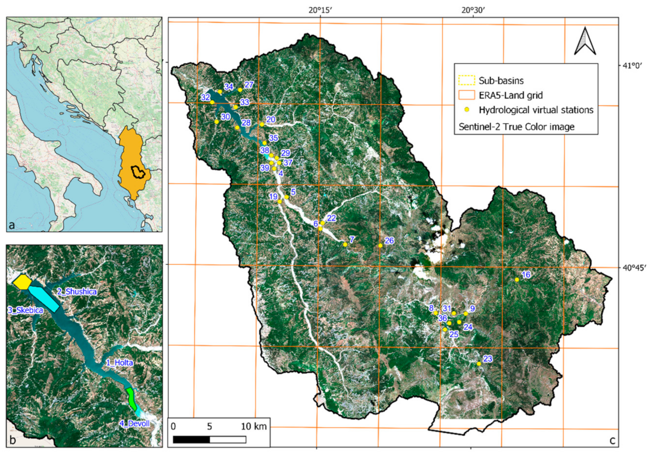
2.1. Study Site

The Banja reservoir is located in the Elbasan district in Albania. With its 14 km² of surface and 400 million m³ of capacity, it is a part of the Devoll Hydropower Project (DHP), which consists of two hydropower plants: the Moglice and Banja plants, intended to increase the power generating capacity of Albania by 17%. The reservoir is formed compounding the Devoll river with a dam 900 m long, 370 m wide, and 80 m high. The Banja hydropower plant has been operational since spring 2016, with an installed capacity of 72 MW and an annual production of 255 GWh.

The Banja catchment considered in this study extends for about 2800 km². It is a hilly-low mountainous environment, with deep valleys at the lowest elevation of less than 50 m a.s.l. and the highest peaks at more than 1500 m a.s.l. Geologically, weak sedimentary rock dominates, which allows strong erosion along the steep slopes. Colluvial and alluvial materials dominate the watershed [26]. The climate is typically Mediterranean, with dry summers and wet winters. Mean annual precipitations range from 800 mm to 1300 mm and mostly fall in November, December, and January. Mean annual temperatures from 12 °C to 13.5 °C have been registered from the beginning of 2000 (https://climateknowledgeportal.worldbank.org/country/albania/climate-data-historical, accessed on 20 December 2022). More than half of the catchment surface is covered by vegetation, both forested lands and shrub/grassland. Thanks to a high variability of rock substrates and soil types, a complex topography and multiple microclimate conditions, there is a high level of biodiversity. Different Natura 2000 Habitats have been identified, with the most representative being a Mediterranean pine forest (with endemic black pine), oak forest, and two quercus forests [27]. The study site is restricted to the Banja watershed included in one single Sentinel-2 tile (Figure 1), with the exclusion of the most eastern part of the catchment, where the land is mostly flat and with low precipitation compared to the rest of the basin [28]. These features make this portion of the catchment less contributory to influencing water quality and hydrological processes of the basin [26]. The time range of investigation considers the first 5 years of the life of the Banja reservoir, from May 2016 (filling of the Banja reservoir started on 15 April) to April 2021.

2.2. Dataset

The dataset used in this study consists of different typologies of data: satellite-derived parameters describing both water and land properties, meteorological forcing, and hydrological variables.

Table 1. List of the used parameters, with relative units, source of data, environmental compartment described, and spatial/temporal characteristics.

Parameter	Acronym	Unit	Source of Data	Environmental Compartment	Spatial Resolution	Temporal Frequency
Chlorophyll-a concentration	Chl-a	µg/L	Sentinel-2 and Landsat 8/9	Water inside the reservoir	10 m/30 m	5/10 days for S2 16 days for L8-L9
Turbidity	Turb	NTU
Secchi Disk Depth	SDD	m
Normalized Difference Vegetation Index	NDVI	-	Sentinel-2	Land/Vegetation	10 m	5/10 days
Enhanced Vegetation Index	EVI	-
Leaf Area Index	LAI	m2/m2
Fractional Cover	FC	%
Snow cover	Snow	%
Total Precipitation	TP	mm	ERA5-Land	Atmosphere	0.1° (11 Km)	hourly
Air Temperature	Tair	°C
Snow Fall	SF	mm
River Discharge	RD	m3/s	HYPE hydrological model	Surface water inside the watershed	27 sub-basins	daily
Sediment Load	SL	kg/day
Runoff Sediment Concentration in local runoff	Ro	mm
	SSCl	mg/L

lists all the parameters, with their acronyms (used hereafter), measure units, data source, the environmental compartment described by the parameter, and the spatial resolution and temporal frequency of data.

The water quality of the reservoir is described by three satellite-derived parameters: chlorophyll-a concentration (Chl-a), water turbidity (Turb), and Secchi Disk Depth (SDD), the latter being the depth at which the 90% of the solar radiation is penetrating inside the water column [29]. The vegetation properties and the sequency of the vegetative seasons is represented through two satellite derived vegetation indices (VI): normalized difference vegetation index (NDVI, [30]) and enhanced vegetation index (EVI, [31]). Vegetation is also described in terms of amount and spatial coverage, using two bio-geophysical parameters: the leaf area index (LAI, [32]) and fractional cover (FC), which is the percentage of vegetation covering the ground with the vertical projection of its canopy elements [33]. The meteorological variables are provided by the meteorological model ERA5-Land from ECMWF (European Centre for Medium-Range Weather Forecasts, [34]) and comprise total precipitation (TP), which includes both liquid and solid precipitations, air temperatures (Tair) measured at 2 m above ground see level, and snow fall (SF), which is the amount of water deriving from the melting of the snow cover (https://cds.climate.copernicus.eu/cdsapp#!/dataset/10.24381/cds.e2161bac?tab=overview, accessed on accessed on 20 December 2022). Finally, the Hydrological Predictions for the Environment (HYPE) model ([35]) is used to produce river discharge (RD), sediment load inside riverstreams (SL), runoff (Ro), and sediment concentration in local runoff (SSCl) for each of the 27 sub-basins composing the considered Banja watershed. The temporal frequency shown in Table 1 is the frequency at which each parameter is provided. Further processing is conducted to homogenize the time step of the variables, i.e., to have both hydrological and meteo parameters at the same daily time step. Figure 2 shows the processing steps used to derive each of the water quality, land/vegetation, hydrological, and meteorological parameters.

As shown in Figure 2, the retrieval of the parameters describing each environmental compartment is complex and involves the use of different software and processors purposely built for the elaboration of satellite images (e.g., Sen2r or SNAP), as well as commonly used tools for statistical analysis (e.g., R). In the following paragraphs, each processing step is described in detail following this structure: retrieval of satellite derived parameters (Section 2.2.1), modelling of hydrological parameters (Section 2.2.2), synthesis of meteorological variables (Section 2.2.3), and statistical analysis (Section 2.2.4).

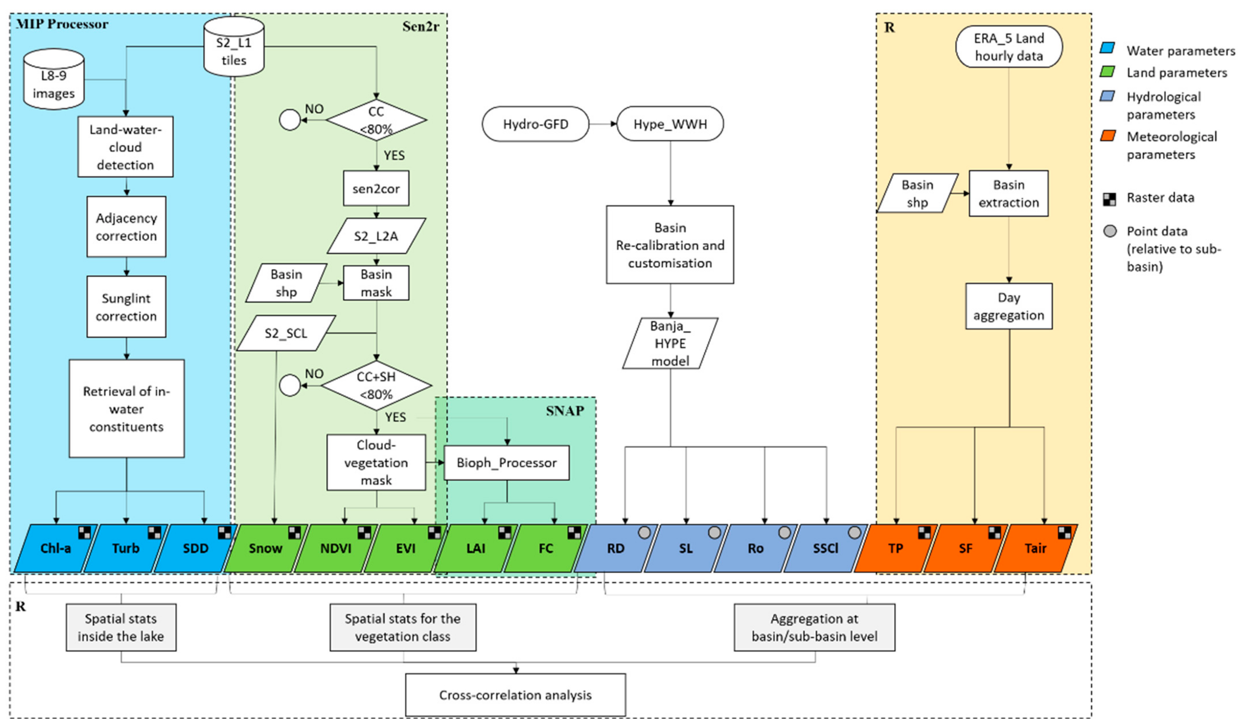
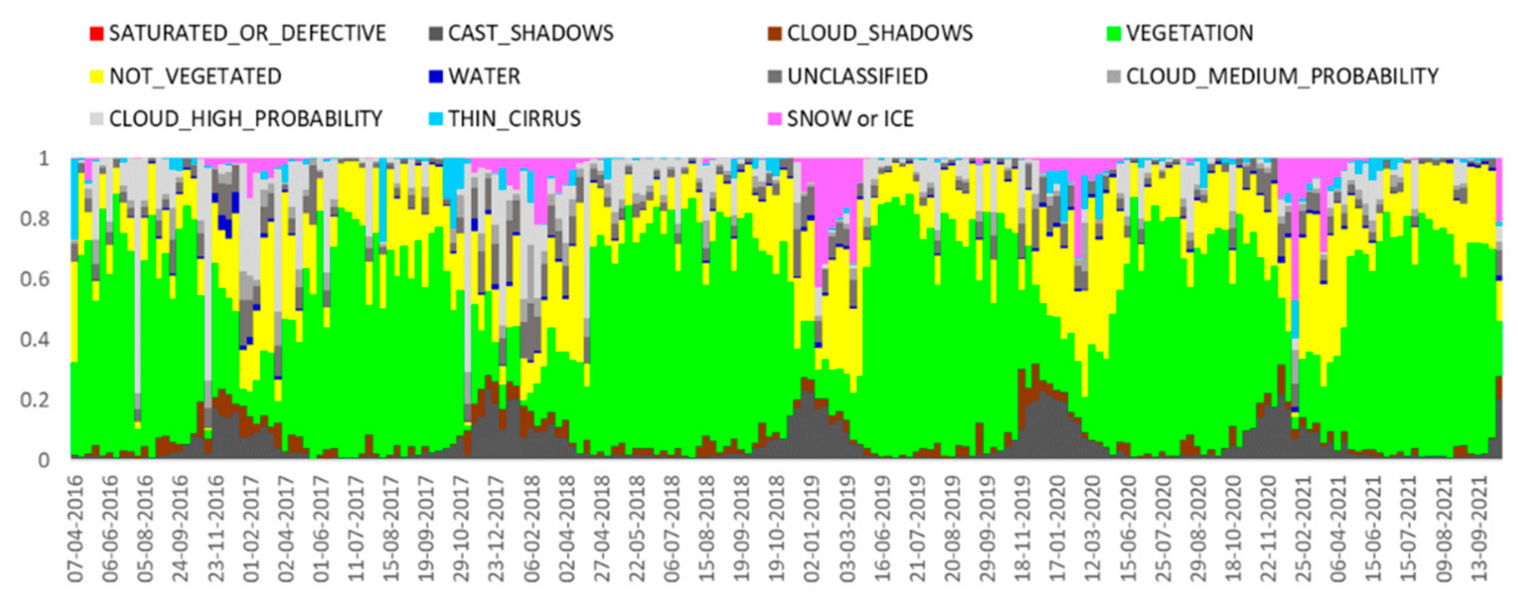
2.2.1. Satellite-Derived Parameters

Sentinel-2 data were made available using the Copernicus Programme (https://scihub.copernicus.eu/, accessed on accessed on 20 December 2022). The Sentinel-2 mission is constituted by a constellation of two identical polar-orbiting satellites (S2A and S2B) placed in the same Sun-synchronous orbit, phased at 180° to each other. The geometry of the system allows the observation of the same portion of the Earth’s surface every 5 days, regardless of the cloud cover. This temporal frequency is guaranteed since the launch of the S2B satellite, which occurred on 7 March 2017, while along with the presence of the single S2A satellite (launched in 2015), the revisiting time was double (10 days). Images are acquired by the MultiSpectral Instrument (MSI), which registers electromagnetic radiation in 12 spectral bands within the visible-shortwave infrared range. Landsat 8/9 data were made available using the longest continuous NASA/USGS satellite program, which started in 1972. The 30 m spatial resolution and the optical bands of the multispectral sensors mounted on the Landsat satellites are a good compromise for tracking the evolution and climate change impacts on both land and water applications.

Sentinel-2 Level 1 tiles (S2_L1) and Landsat 8/9 images (L8-9) covering the Banja watershed (Figure 1) were ingested by the Modular Inversion and Processing System (MIP, [36]), which is a physically based processor able to solve the electromagnetic transfer through the atmosphere, the air/water interface, and the waterbody. With the implementation of radiative transfer models, the MIP can “translate” radiance values registered by a satellite sensor into the concentration of in-water constituents and other water quality products through a multi-layer system of elaboration steps, including the elimination of adjacency and sun-glint effects, the atmospheric correction, and the modelling of the in-water constituents and land-water-cloud masking. The software version of MIP is fully based on physics and relates absorption and backscattering of in-water properties as a function of the sensor radiances. The accounted dependencies contain variable target level altitude and observer altitude, variable atmospheric aerosol properties, amongst other parameters, using the radiative transfer model by means of a finite element model. The outputs of the MIP can be manifold; here we consider Chl-a, Turb, and SDD (Figure 2). In addition, MIP generates quality indicators and performs a quality control useful for evaluating which images present problems and consequently removing them from the data-set. MIP water quality products have been validated in different works showing good quality (e.g., [37]).

A combination of Sen2r R library and SNAP software were used for the retrieval of land/vegetation parameters. Sen2r ([37], https://sen2r.ranghetti.info/, accessed on accessed on 20 December 2022) has been built for searching, downloading, and pre-processing Sentinel-2 optical images in an easy and well-organized way, thanks to a clear and immediate graphical interface. The Sentinel Application Platform (SNAP), complete with Sentinel Toolboxes, is an open access platform purposely built for the elaboration of Sentinel images, even if it can analyze many different types of satellite images. S2_L1 images were filtered for cloud coverage (CC) less than 80% (which is the tile surface out of the watershed) in order to dispose of the larger dataset available. S2 images were then corrected for the atmospheric effects using the sen2cor code and masked for the outside of the considered catchment (Figure 1). Images were then further filtered using the scene classification map (SCL) product provided within the S2_L2 processing level (Figure 3). Images with more than 80% of “disturbing effects” such as clouds (e.g., cirrus + medium and high probability clouds), shadows (e.g., cloud shadows + cast shadows) and unclassified pixels were rejected.

This choice excludes those images greatly affected by cloud coverage, as well as those images in which the vegetation class is reduced in extent due to topographic effects and not to phenological cycles. As it can be observed looking at Figure 3, a recurrent increase of cast shadows occurs along the fall–winter months, when the sun-sensor-target geometry can lead to shaded slopes in mountain and hilly environments. This fact can somehow ‘hide’ shaded vegetation surfaces, with consequences on the estimation of vegetation indices and bio-physical parameters, which are derived from the vegetation class only in this work. A total number of 204 images turned out to be suitable for the following processing steps. The NDVI and EVI maps were then extracted for SCL vegetation surfaces for all dates respecting the cloud + shadows conditions explained above, using the sen2r library. Any possible error in the masking procedure (e.g., some pixels still affected by atmospheric or shadow effects at the boundaries of the cloud/shadow mask) was eliminated by setting NDVI and EVI thresholds at 0.2 (minimum value) and 1 (maximum value).

LAI and FC maps, instead, were obtained using the SNAP software and the implemented biophysical processor S2_10m, which derives biophysical variables from top-of-canopy normalized reflectance S2 data. The tool implements neural networks algorithms for the retrieval of LAI and FC values and provides quality bands for each parameter as well. The cloud + shadow mask was applied equally to both VIs products (NDVI and EVI) and bio-physical parameters (LAI and FC).

Based on the SCL_S2 product, the snow cover was derived as relative percentage of snow and ice class over the Banja catchment (Snow in Figure 2).

2.2.2. Hydrological Parameters

The HYPE model is a semi-distributed process-based model capable of simulating hydrological processes from a single basin to a global scale. The HYPE model for the Banja watershed was developed from a global application of HYPE, World Wide HYPE (WWH, [38,39]) by extracting a submodel from WWH and refining spatial resolution and process description. The refined model, Banja–HYPE, specifically includes the effects of karstic bedrock and aquifers which dominate hydrology at this catchment [40]. Banja–HYPE uses the same meteorological forcing data from the Hydrological Global Forcing Data set (HydroGFD, [41]) as WWH. The Banja–HYPE model consists of 39 sub-basins, 27 of which are located upstream of the dam and thus are considered in this study. The calibration process took advantage of historical discharge data at 8 sites (from 1979 to 1985–1995 depending on the site) available within the entire catchment, as well as EO data such as fractional snow cover (ESA CCI, European Space Agency Climate Change Initiative, https://climate.esa.int/en/projects/snow, accessed on accessed on 20 December 2022), actual evapotranspiration, and potential evapotranspiration (the MODIS global evapotranspiration products, [42]). Preliminary calibration of sediment concentrations was conducted with historical suspended sediment concentrations monitored at 3 sites (Kokel, Kozare, and Gjinikas) from 1979 to 1985–1996 depending on the site. An additional 2 years of sediment concentrations were available at one site (Kokel) for a more recent period (2016–2018). The Kling–Gupta Efficiency (KGE) was between 0.35 and 0.68 for discharge and between −0.11 and 0.49 for sediment. Relative error varied between 13.2–53.8% and −9.9–58% for discharge and sediment, respectively.

The Banja–HYPE model was executed with daily precipitation and air temperature from HydroGFD for 1979–2021. Timeseries of RD, SL, Ro, and SSCl were retrieved for the 27 sub-basins included in our study site (Figure 1) for the period May 2016–April 2021.

2.2.3. Meteorological Variables

Meteorological parameters were downloaded from the Copernicus Climate Data Store ([34], https://cds.climate.copernicus.eu/cdsapp#!/dataset/10.24381/cds.e2161bac?tab=overview, accessed on accessed on 20 December 2022) and belong to the ERA5-Land dataset. ERA5-Land is a reanalysis of ERA5 data, which combines model data with in-situ observations. It provides global gridded data at a spatial resolution of 0.1° × 0.1° (see Figure 1) at hourly time steps from 1950 to present. For the purposes of this work, three meteorological parameters were selected, namely the TP (m, then converted into mm), which corresponds to the liquid and frozen water (rain and snow) that falls to the Earth’s surface; the SF (m, then converted into mm), which is the equivalent water coming from the melting of snow; and Tair (K, then converted into °C), which is the air temperature at 2 m height above the land surface. The ERA5-Land gridded products were extracted for the entire Banja watershed and aggregated at daily timesteps (within the R environment) in order to be comparable with the hydrological parameters and with the water/land/vegetation variables.

2.2.4. Statistical and Spatial Analysis

Spatial statistics (i.e., mean, minimum, maximum, and percentiles) were calculated for all the raster products (Figure 2). For the water quality parameters, statistics were calculated inside a representative polygon in the central part of the Banja reservoir (cyan polygon in Figure 1). This polygon was chosen in a way to avoid high variations which can occur near the inflows as a result of the different contributions from the single sub-basins around the reservoir. The spatial variability of water quality parameters inside the reservoir was evaluated through the use of two further polygons, where spatial means were calculated (yellow and green polygons in Figure 1, namely dam and inflow virtual stations).

As for vegetation parameters, statistics were calculated over the vegetation class covering the entire basin. Each of the vegetation parameters was weighted for the percentage of vegetation cover within the basin, derived from the S2-SCL classification product.

As for meteorological parameters, statistics were calculated over the entire watershed considered as the study site (Figure 1c).

As for hydrological parameters, daily RD and SL estimations for those sub-basins entering the Banja reservoir (i.e., virtual stations 4, 37, 38, 29, 35, 20, 33, 27, 34, 32, 30, 28, and 39 in Figure 1) were summed. Average Ro over the catchment was calculated as area-weighted average for all sub-basins included inside the watershed (represented by the 27 virtual stations in Figure 1), as shown in Equation (1).

$$\mathrm{Ro}=\frac{\sum {(\mathrm{Ro}}_{\mathrm{i}}·{\mathrm{A}}_{\mathrm{i}})}{\sum {\mathrm{A}}_{\mathrm{i}}}$$

(1)

where ${\mathrm{Ro}}_{\mathrm{i}}$ is the specific runoff of each sub-basin $\mathrm{i}$, and ${\mathrm{A}}_{\mathrm{i}}$ is the relative area in m². SSCl was averaged over the watershed following Equation (2).

$$\mathrm{SSCl}=\frac{\sum \left({\mathrm{Ro}}_{\mathrm{i}}·{\mathrm{A}}_{\mathrm{i}}·{\mathrm{SSCl}}_{\mathrm{i}}\right)}{\sum {(\mathrm{Ro}}_{\mathrm{i}}·{\mathrm{A}}_{\mathrm{i}})}$$

(2)

where ${\mathrm{SSCl}}_{\mathrm{i}}$ is the sediment concentration in local runoff of sub-basin $\mathrm{i}.$ A unique timeseries with the total amount of matching dates in which all the parameters were available was built, and a cross-correlation analysis was performed using R.

A special focus was placed on particular meteorological events or short periods, in order to analyze in more detail the spatial variability of water turbidity inside the Banja reservoir, test the potentialities of EO-derived water quality (WQ) data to describe such variability, and try to provide explanations for possible differences for each single case. For these specific analyses only the Turb parameter was considered, since it is the most relevant to the water quality of the Banja reservoir.

3. Results

As the output of the methodological process, 154 observations came out complete of all the considered parameters, that is, water, land, hydrological, and meteorological parameters. An average of 30 observations are present every year, with exceptions for 2016 and 2021, which are not complete, since the Banja reservoir became operational in April 2016, and hydrological data are available only until the end of April 2021. The most represented months are July to October, with 17 to 21 total observations (average of 4–5 per month). This is most likely due to the local Mediterranean climate, with dry summers and more rainy winters. During this season the cloud coverage can prevent optical satellite acquisitions, thus reducing the number of observations during this period. Results about the temporal trend of each parameter are described in the following Section 3.1, while results about the cross-correlation analysis are reported in Section 3.2. Section 3.3 presents a particular focus on specific events causing spatial and temporal changes in the water quality within the reservoir.

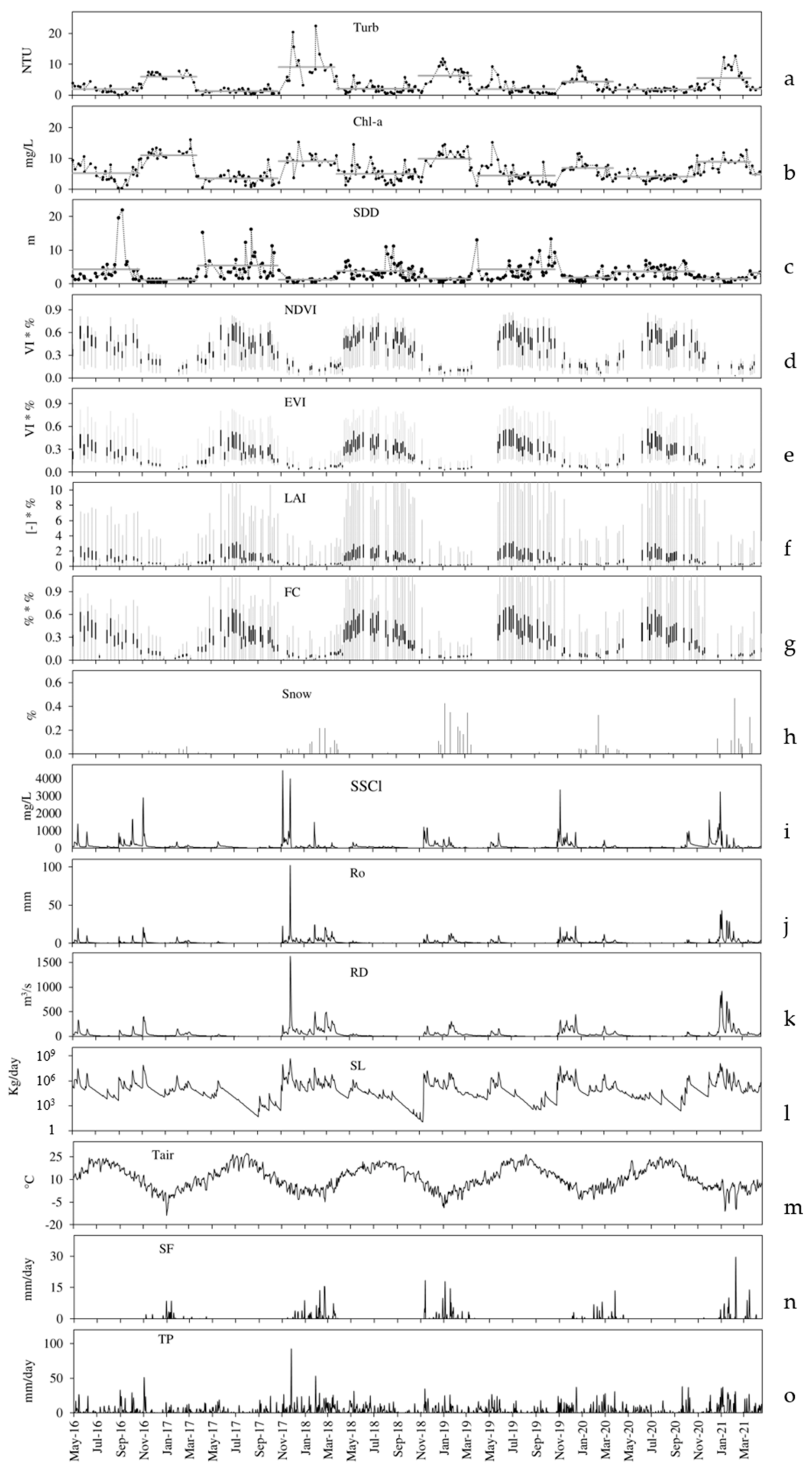
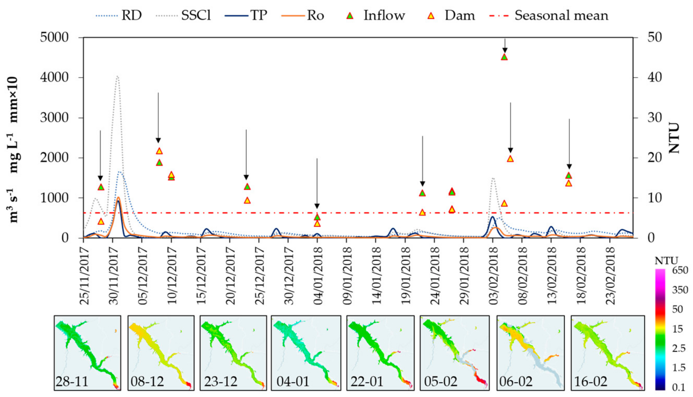
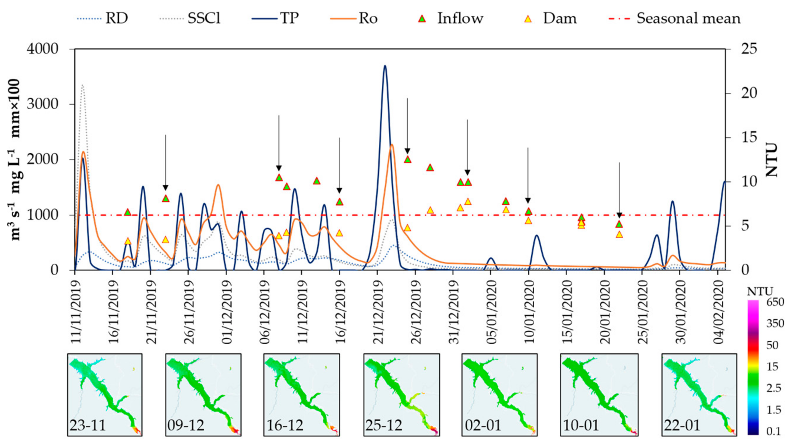
3.1. Temporal Series

Figure 4 shows the temporal series of each water quality, land, meteorological, and hydrological parameter. The common temporal range considered stretches from 7 May 2016 (first date of S2 overpass over the completely filled Banja reservoir) to 24 April 2021 (when hydrological simulations stop). The first three plots (Figure 4a–c) show the EO derived water quality parameters Turb, Chl-a, and SDD as retrieved by the MIP processor (see Section 2.2.1 and Figure 2) for a central polygon of the Banja reservoir (Figure 1). The water quality timeseries consists of 375 values within the time range considered, since S2 acquisitions were increased with good quality Landsat 8–9 acquisitions (Figure 2, Table 1). In this way, it is possible to have a denser dataset, which is good for appreciating temporal variations of the observed parameters. All three parameters show a seasonal behavior, with higher values during autumn–winter and lower values during spring–summer for Turb and Chl-a, while SDD shows an inverted trend, since it is notoriously influenced and reduced by the presence of dissolved and suspended substances inside the water column. Maximum averages along the autumn–winter season range around values of 6.25 NTU and 9.14 mg/L for Turb and Chl-a respectively, while minimum averages range around 1.82 NTU and 4.49 mg/L during the spring–summer season. At the same time SDD moves around minimum values of 1.42 m during autumn–winter, to its average maximum values around 4.11 m during spring–summer. These trends suggest that the temporal variability of water quality inside the Banja reservoir is strongly influenced by a seasonal phenomenon. Besides the seasonal trend, some relative peaks are visible along the years. In particular, a strong increase in Turb is registered during December 2017 and February 2018, with NTU values above 20. Other minor increases (around 10 NTU) of Turb are recurrently observed during January of each considered year. Instead, relative peaks of Chl-a occur mostly during March (2017, 2019, and 2021), May (2018 and 2019) or even December (2017, 2019, and 2020) or January (2019, 2020, and 2021). SDD shows high peaks generally during spring–summer, e.g., April and August 2017, 2018, and 2019. The maximum value of SDD is registered in September 2016, some months after the operativity of the Banja dam.

Timeseries of vegetation parameters are shown from Figure 4d–g. Each boxplot corresponds to weighted (see Section 2.2.1) statistics calculated over the vegetation class in each single S2 acquisition. The black box covers the 25th to 75th quantile, while grey lines connect to minimum and maximum values. A denser frequency in the data is visible from spring 2017, when the S2B satellite was launched. Some data gaps are observable in January 2017, June–July 2018, April–May 2019, and May–June 2020, when persistent cloud cover prevented the analysis of satellite images. Both spectral vegetation indices (i.e., NDVI and EVI) and biophysical parameters describing the vegetation cover (i.e., LAI and FC) show the same behavior, which reflects the phenological cycle of annual vegetation. Maximum daily spatial means are achieved in June/July, with values of 0.65 for NDVI, 0.45 for EVI, 2.05 for LAI, and 0.55 for FC. Minimum daily spatial means occur, instead, from December to February and are around 0.1 for NDVI, 0.04 for EVI, 0.17 for LAI, and 0.04 for FC. It has to be noted that these values are multiplied for the percentage of land occupied by vegetation inside the watershed. In this way, spatial average values of the vegetation parameters are scaled to the occurrence of the vegetation cover in the catchment. Differentiation between evergreen and deciduous species was not performed, since it requires more in-depth knowledge of vegetation associations inside the catchment. The snow timeseries (Figure 4h) is in accordance with the SF timeseries (Figure 4n), which makes both parameters derived from different sources, but related to the same phenomenon, reliable.

Hydrological parameters’ timeseries are shown in Figure 4i–l. Relative peaks recur in each timeseries, since these parameters are forced by the same meteo-climatological conditions. Absolute high peaks usually occur in the autumn–winter seasons, corresponding to the period when the major contribution of total precipitation occurs. Relative peaks are present in spring, with annual oscillations (i.e., peaks more visible in 2019 and 2020). An exceptional rain event is observable in December 2017, when TP reach a value of 92 mm day⁻¹, and consequently, RD increased to 1630 m³s⁻¹, Ro > 100 mm, SSCl to about 4400 mg L⁻¹, and SL up to 4.6 × 10⁸ Kg day⁻¹ in one day, the 1st of December. Other consistent increases in the hydrological parameters are observable in November 2018–February 2019 (around 200 m³s⁻¹ for RD, ~10 mm for Ro, up to 1000 mg L⁻¹ for SSCl, ~5 × 10⁶ Kg day⁻¹), November-December 2019 (RD > 300 m³s⁻¹, Ro > 20 mm, SSCl > 3300 mg L⁻¹ and SL >6 × 10⁷ Kg day⁻¹), and January 2021 (>900 m³s⁻¹ for RD, ~40 mm for Ro, up to 3200 mg L⁻¹ for SSCl and 1.27 × 10⁸ Kg day⁻¹ for SL), while minor events are registered in May-June 2019 (up to 100 m³s⁻¹ for RD, >5 mm for Ro in June only, >850 mg L⁻¹ for SSCl and 1 × 10⁶ Kg day⁻¹ for SL) and March–April 2020 (>100 m³s⁻¹ for RD, 7 mm for Ro in March, >250 mg L⁻¹ for SSCl in March and 9.6 × 10⁵ Kg day⁻¹ for SL).

Series of meteorological variables are plotted in Figure 4m–o. Tair shows a rather Mediterranean behavior, with marked seasonality and maxima during summer (around 21–22 °C in July–August) and minima in winter (0 °C or some degree below 0 °C in January). Rainy precipitations occur mainly in autumn and spring, with winter snowfalls making a continuum TP increase during November to May. Annual SF range from 55 mm to 158 mm. Minimum SF and snow cover are observed during the 2016–2017 winter season, while longer and more snowy seasons are those of 2017–2018, 2018–2019, and 2020–2021. In particular, in 2017–2018 SF is higher during the end of winter (up to 88 mm in February 2018), while in 2018–2019 snowy precipitations are higher in autumn–winter (28 mm registered during November 2018 and 83 mm in January 2019). Late snowfalls are observed in spring 2018, 2020, and 2021. Annual TP varies from 904 mm in 2020 to 1422 mm in 2018. The year 2021 has a relatively exceptional wet January with 352 mm of TP, while the highest monthly values are always below 250 mm. The year 2018 registers more than 150 mm of TP in four months (February, March, May, and June). The year 2017 shows the wettest December, with 209 mm of TP, half of which fell on 1 December.

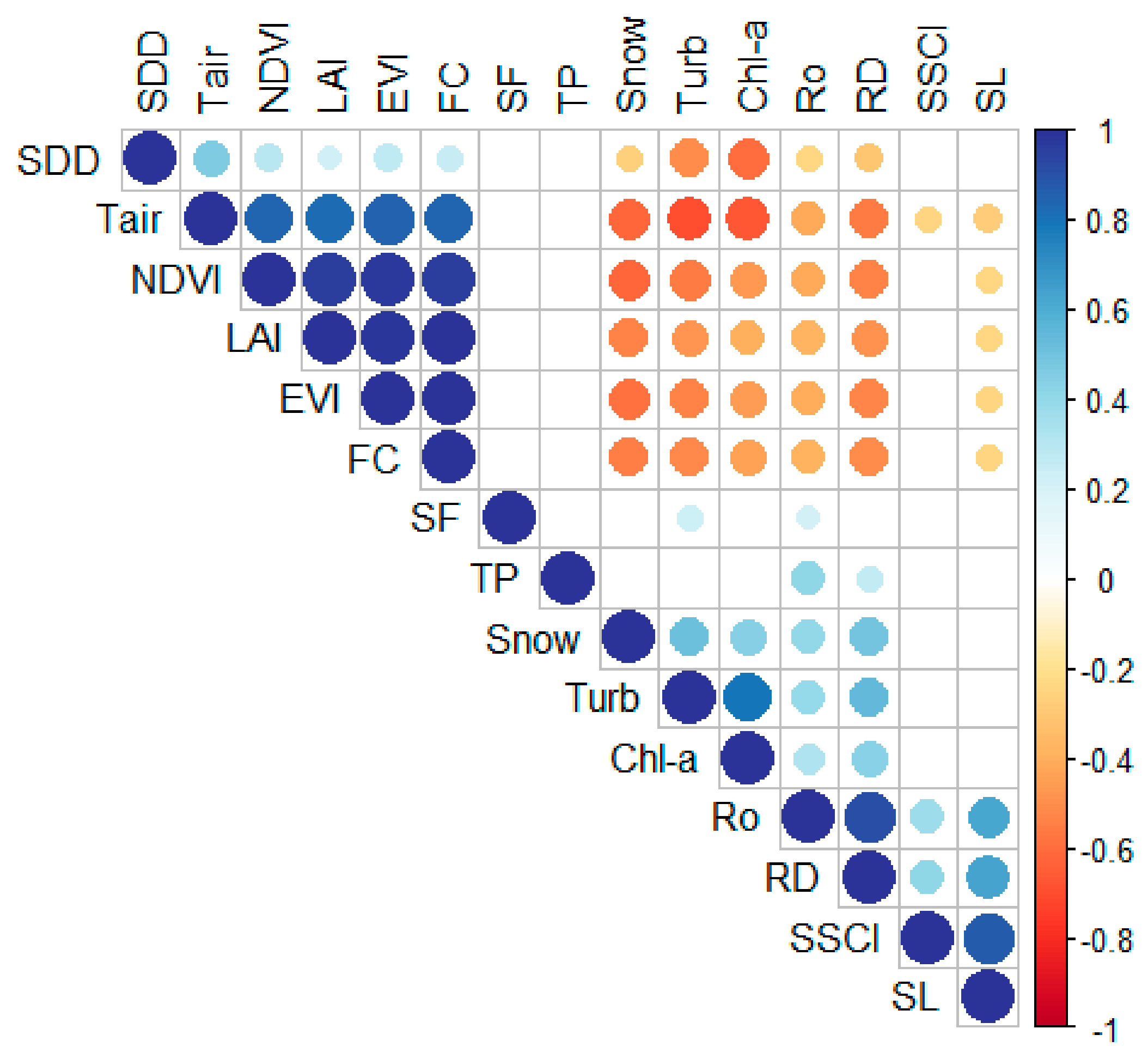
3.2. Cross Correlation

The result of the cross-correlation analysis of all the water quality, land/vegetation, hydrological, and meteorological parameters is shown in Figure 5.

Positive correlations are represented with bluish colors, while negative correlations with reddish colors. Points are proportional to the correlation coefficient and not statistically significant correlations, for which p > 0.01, are blank. Parameters belonging to the same water group, such as water quality or vegetation group (e.g., Turb, and Chl-a or NDVI, EVI, LAI and FC), are positively correlated (> 0.5 corr coeff for water quality parameters, >0.9 corr coeff for vegetation parameters). Hydrological variables are generally negatively correlated with vegetation descriptors (with a greater correlation for RD (<−0.49) and Ro (<−0.37)), which in turn are negatively correlated with water quality parameters (from −0.48 to −0.55 for Turb and from −0.39 to −0.46 for Chl-a). This leads to a positive correlation between hydrological variables and water quality parameters (0.4 corr coeff between Turb and Ro and 0.55 between Turb and RD). Snow and SF are negatively correlated with vegetation descriptors (from −0.53 to −0.61 for snow and from −0.15 to −0.17 for SF, but with no significant correlation) and positively correlated with water quality parameters (0.51 and 0.24 respectively with Turb, and 0.44 corr coeff between snow and Chl-a) and hydrological variables (0.41 with Ro and 0.49 with RD for snow, and 0.22 with Ro). SDD is slightly positively correlated with vegetation descriptors (corr coeff from 0.22 to 0.29) and slightly negatively correlated with hydrological variables (−0.24 corr coeff with Ro and −0.3 corr coeff eith RD). Tair is positively correlated with SDD (0.46 corr coeff) and with vegetation descriptors (>0.8), while it is negatively correlated with Turb (−0.69) and Chl-a (−0.66). TP has a positive significant correlation only with Ro (0.42) and RD (0.27). SSCl is significantly correlated only with Tair (−0.24) and with Ro and RD (0.38 and 0.41, respectively). SL has slight but significant negative correlations with vegetation descriptors (from −0.23 to −0.25) and Tair (−0.28), and strong positive correlations with Ro, RD, and SSCl (>0.6).

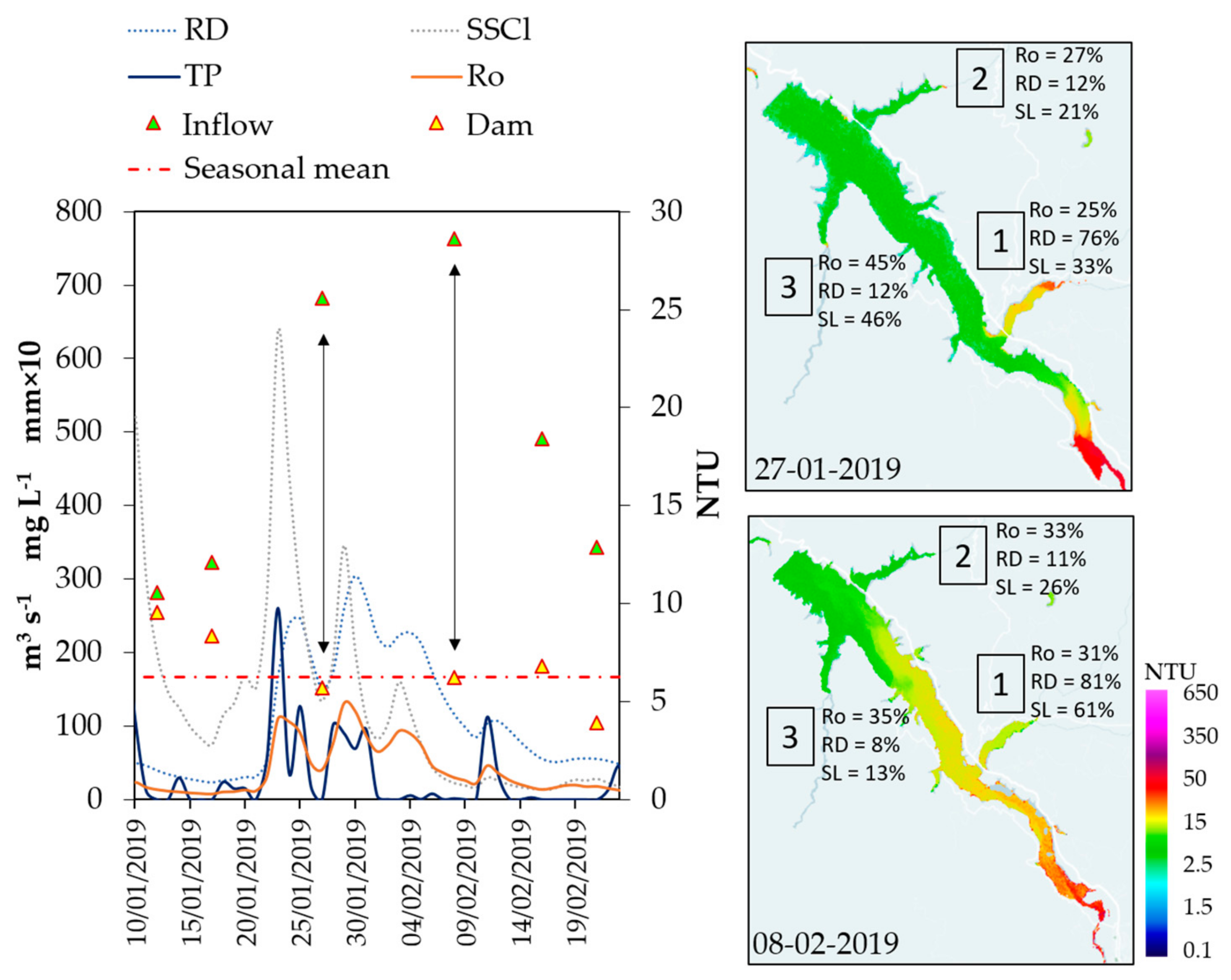
3.3. Analysis of Turbidity Spatial Patterns during Specific Events

In this section, particular periods and events are analyzed in detail to highlight and explain spatial patterns in the Banja reservoir. For the following examples the Turb parameter is the only water quality parameter considered, since the accumulation of sediments is the main issue the reservoir is facing.

The exceptional rain event that occurred in November 2017 caused a sudden increase and homogenization of reservoir turbidity. It can be observed in Figure 6 that Turb near the inflow of the Devoll river (green triangles), compared to Turb near the dam (yellow triangles), are quite similar after (first image available on 8 December 2017) the heavy rain (92 mm in one day) that fell on 1 December 2017. In addition, the two values progressively decrease at the same rate (i.e., both still above the seasonal mean 22 days after the event) until they drop below the seasonal mean 35 days after the rain event. This suggests a persistent spatial homogeneity of Turb inside the reservoir, as can be observed by looking at the Turb maps of Figure 6. As for the precipitation event, this is an extreme situation, while the most common condition is a spatial difference between Turb at the inflow and Turb at the dam (e.g., see maps on 28 November 2017 and 05 February 2018), with an average difference of 8 NTU and peaks >30 NTU recurring in late winter (February and March). For instance, the more moderate rains of 2–4 February 2018 (about 82 mm in total) magnify this difference, which takes 12–13 days to disappear. In this case, the satellite acquisition is on 5 February 2018, one day after the rain event, which is why the increase in Turb is more consistent compared to November 2017. Furthermore, thanks to another satellite acquisition on 6 February 2018, it can be observed that suspended sediments coming from the main inlet (Davoll river) take 3 days to reach the dam.

The autumn–winter season 2019–2020 (Figure 7) is mainly characterized by a spatial differentiation between inflow and dam Turb values, a condition fostered by moderate (>10 mm in one day) and relatively frequent (every 5–10 days) rainfalls. The persistence of the rain, even if moderate, favors the progressive mobilization and transport of sediments in the watershed, and their accumulation at the main inflow of the reservoir. It is interesting to see that after the heaviest event of the season (37 mm on 23 December 2019 preceded and followed by one day with 15 mm of TP), the difference between Turb averaged at the two virtual stations of the reservoir (inflow and dam) is gradually disappearing, first due to an increase in the dam station and then to a decrease in both the stations. It takes 25 days in the absence of precipitation to erase the Turb difference between the two stations and bring the Turb values back below the seasonal average.

The spatial variability of the water quality within the Banja reservoir changes relatively fast and depends on tributary contributions. Figure 8 shows a case in which, although the difference in Turb between the two virtual stations (Inflow and Dam) is very similar, Turb maps show different spatial patterns. These spatial patterns can be explained considering how Ro, RD, and SL are spatially distributed in the sub-basins around the reservoir. If we express Ro, RD, and SL through their relative percentage for each inflow, excluding the main one (Devoll river), which always contributes the most to the supply of sediments in the reservoir (more than 70%), we can see that there is a gradual increase of Ro, RD, and SL in the contribution of sub-basin one (Holta inflow). In particular, the SL contribution on 8 February is double the one on 27 January. Here, two rivers join in the Holta river and enter the reservoir. The doubled RD favors the transport of sediments within the river waters, spreading along the majority of the reservoirs. Shushica and Skebica rivers, instead, have a small contribution to the supply of sediments inside the reservoir.

4. Discussion and Practical Application

Water quality parameters inside the Banja reservoir have seasonal trends, as can be observed in Figure 4. This is a common finding, which has to be defined case by case, where different climatic conditions and abiotic/biotic interactions affect the shift of maxima and minima in different periods [43]. Water turbidity and Chl-a concentration often present similar trends, because terrestrial loads, especially from agricultural and urban runoff, enrich waters with nutrients, increasing their productivity [44,45]. Peaking periods can vary regionally, because of the occurrence of the rainy season in different periods for tropical [1,45] or equatorial, or Mediterranean climates. In the Banja reservoir catchment, the seasonal trend of water quality parameters (mainly Turb) depends on a combined effect of meteorological factors and vegetative cycles. Precipitation, even if it does not display marked seasonality in this catchment, is more frequent during the autumn–winter season (when snowy events also take place), and at the same time, the vegetation cover is reduced to evergreen species, decreasing its protective action on soil erosion. This is further confirmed by the negative correlation between Chl-a/Turb and Tair, and between Chl-a/Turb and vegetation descriptors (NDVI, EVI, LAI, FC; Figure 5). Rain interception by vegetation components (i.e., leaves and stems) is considered of great importance for hydrological modelling; indeed it has been incorporated into mathematical models describing matter transport during rainfall events [46]. The link between the vegetation presence within the catchment and water turbidity in rivers and lakes/reservoirs has been reported by others [7,47] and is made more evident here by the lower occurrence of rains during the vegetative season. The absence of a significant correlation between TP and water quality parameters may be explained by the fact that precipitation event impacts on water quality are mediated by the presence or absence of a “protective” vegetation layer. The significant positive correlation between snow and Chl-a/Turb (Figure 5) demonstrates that even snowmelt has an impact on the water quality of the reservoir, as already pointed out by Mouris et al. [48].

Besides the seasonal temporal trend, turbidity is also influenced by the occurrence of events of short duration and particular intensity, as highlighted in Section 3.3. Moreover, these events can lead to a different spatial distribution of turbidity within the reservoir. Intensity and persistence of rain events leads to high runoff erosion and sediment transport [49,50]. The shape and morphology of a reservoir also affect spatial variations in water quality. Large, deep lakes are less influenced by the consistent tributary sediment loads, because of high dilution capabilities, and turbidity plumes can be limited to regions close to tributary mouths or embayment ([51,52]). On the other hand, narrow, elongated and relatively shallow water bodies are more strongly influenced by the input of suspended material during precipitation, and changes in water quality may affect the water body as a whole. It has also been observed that events that shift from a more typical lacustrine regime to a fluvial one are possible in the same reservoir [53]. The Banja reservoir is an elongated narrow reservoir (since it was created by impounding the Devoll river), with relatively shallow depths (mean depth of 12 m [54]), extending with multiple arms into surrounding small valleys and sub-catchments. This morphometry makes it prone to show high spatial variability in water turbidity after precipitations, as seen in Figure 6, Figure 7 and Figure 8. Furthermore, poorly aggregated soils located along slopes are one of the reasons why the Devoll catchment experiences extremely high rates of erosion, and sediment yields which are comparable to the Himalayan mountains [55].

High temporal and spatial variability of water turbidity, associated with the significant amounts of sediment involved, make the management of the hydropower plant particularly challenging. In this framework a good and site-specific strategy for managing reservoir sedimentation can improve the performance of the system and the efficiency of management operations [56,57]. An accurate evaluation of forcing variables and local dynamics which take place in a specific basin is the starting point for building an efficient management plan. The most accurate possible analysis of the local situation can be achieved only integrating different data sources, with the best spatial and temporal detail attainable. The spatial information obtained for instance in the three specific periods analyzed in Section 3.3 is of undoubted value for choosing the best location both for monitoring stations and for specific management actions, which may prevent sediment accumulation localized near the dam and the engineering components of the hydropower plant. Moreover, the periodicity of the information makes it possible to follow the evolution of the phenomena (Figure 6 and Figure 7) and even retrace them in the past (as performed in this work) in order to have a robust database on which to plan future maintenance and operation actions.

This work demonstrates the efficiency of the integrated use of multi-source data for the study and characterization of the water quality of an artificial reservoir. The integration of different types of data (derived from satellite or from meteorological and hydrological models) makes it possible to follow and explain the temporal and spatial variations of the water quality parameters of the Banja reservoir. This approach finds its main application in the management of water resources for the production of hydroelectric energy, and in particular in the framework of the HYPOS (HYdro-POwer-Suite) H2020 Project. The results obtained through the processing of the different types of data first of all increase the number of available measurements relating to a certain parameter compared to a traditional sampling method. For example, the water turbidity value derived from satellite images is spatially distributed for more than 18,500 points and for more than 171,000 points on the surface of the Banja reservoir in one single day, depending on whether an L8/9 or S2 image is used. The counterpart is represented by the fact that this amount of data cannot be available every day, but it is dependent on satellite acquisition orbits and on sky conditions. However, it is an important advantage compared to the traditional measurement campaigns carried out with significant economic and personnel efforts, which cannot in any case cover the amount of data gathered by a satellite acquisition. Secondly, the use of different multi-source data allows a more complete view of the hydrological processes that occur inside the entire river basin, while through traditional management approaches, understanding remains limited to what happens at the single points of measurement of the variables of interest (e.g., water flow or sediment load measured at a fixed gauge station). Furthermore, it has been calculated that the adoption of an integrated system of measures (such as the one presented in the article) for the management of a hydroelectric energy production plant turns out to be incredibly cheaper than traditional management methods (the cost is reduced to 12.5%).

5. Conclusions

Integration of multi-source data allowed the finding of the multiple relations that exist among the different parameters which describe the water quality of a catchment. This integrated vision has highlighted the complexity of the phenomena that can influence the water quality of a reservoir. It has been observed that the water quality varies greatly both temporally and spatially within the reservoir and that this variability cannot be described in absolute terms, but depends in turn on the extent, duration, and location of the meteorological events, as well as on the characteristics of the soil (e.g., presence of vegetation cover) at that time. Further scientific developments can include the evaluation of the contribution of different vegetation species and associations to the hydrology of the watershed, or a more detailed analysis about the hydrological contribution of each single sub-basin to the water quality of the Banja reservoir.

It is necessary to use systems (such as decision support platforms) that allow for the integration of all possible information in order to be able to plan a sustainable and intelligent management of the water resource. In particular, in the context of reservoirs used for the production of electricity, such information is useful for deciding when, where, and which operations are the best ones to be implemented to manage not only the water resource, but also the functioning of the dam (e.g., problem of excessive accumulation of sediments) and ensure the necessary amount of electricity to the downstream population.

References

1. Robert, E.; Grippa, M.; Kergoat, L.; Pinet, S.; Gal, L.; Cochonneau, G.; Martinez, J.-M. Monitoring Water Turbidity and Surface Suspended Sediment Concentration of the Bagre Reservoir (Burkina Faso) Using MODIS and Field Reflectance Data. Int. J. Appl. Earth Obs. Geoinf. 2016, 52, 243–251. [Google Scholar] [CrossRef]
2. Rossi, N.; DeCristofaro, L.; Steinschneider, S.; Brown, C.; Palmer, R. Potential Impacts of Changes in Climate on Turbidity in New York City’s Ashokan Reservoir. J. Water Resour. Plan. Manag. 2016, 142, 04015066. [Google Scholar] [CrossRef]
3. Hsieh, Y.P.; Nemours, D.; Bugna, G. A Field-Scale Soil Erosion Study: An Example from a North Florida Farm. CATENA 2022, 218, 106551. [Google Scholar] [CrossRef]
4. Delia, K.A.; Haney, C.R.; Dyer, J.L.; Paul, V.G. Spatial Analysis of a Chesapeake Bay Sub-Watershed: How Land Use and Precipitation Patterns Impact Water Quality in the James River. Water 2021, 13, 1592. [Google Scholar] [CrossRef]
5. Zhao, Y.; Xia, X.H.; Yang, Z.F.; Wang, F. Assessment of Water Quality in Baiyangdian Lake Using Multivariate Statistical Techniques. Procedia Environ. Sci. 2012, 13, 1213–1226. [Google Scholar] [CrossRef]
6. Dai, X.; Zhou, Y.; Ma, W.; Zhou, L. Influence of Spatial Variation in Land-Use Patterns and Topography on Water Quality of the Rivers Inflowing to Fuxian Lake, a Large Deep Lake in the Plateau of Southwestern China. Ecol. Eng. 2017, 99, 417–428. [Google Scholar] [CrossRef]
7. Zhang, L.; Xin, Z.; Feng, L.; Hu, C.; Zhou, H.; Wang, Y.; Song, C.; Zhang, C. Turbidity Dynamics of Large Lakes and Reservoirs in Northeastern China in Response to Natural Factors and Human Activities. J. Clean. Prod. 2022, 368, 133148. [Google Scholar] [CrossRef]
8. Li, X.; Zhang, Y.; Ji, X.; Strauss, P.; Zhang, Z. Effects of Shrub-Grass Cover on the Hillslope Overland Flow and Soil Erosion under Simulated Rainfall. Environ. Res. 2022, 214, 113774. [Google Scholar] [CrossRef]
9. Moreno Madriñán, M.J.; Al-Hamdan, M.Z.; Rickman, D.L.; Ye, J. Relationship Between Watershed Land-Cover/Land-Use Change and Water Turbidity Status of Tampa Bay Major Tributaries, Florida, USA. Water, Air, Soil Pollut. 2012, 223, 2093–2109. [Google Scholar] [CrossRef]
10. Hou, X.; Feng, L.; Duan, H.; Chen, X.; Sun, D.; Shi, K. Fifteen-Year Monitoring of the Turbidity Dynamics in Large Lakes and Reservoirs in the Middle and Lower Basin of the Yangtze River, China. Remote Sens. Environ. 2017, 190, 107–121. [Google Scholar] [CrossRef]
11. Liu, J.; Yang, H.; Gosling, S.N.; Kummu, M.; Flörke, M.; Pfister, S.; Hanasaki, N.; Wada, Y.; Zhang, X.; Zheng, C.; et al. Water Scarcity Assessments in the Past, Present, and Future. Earth’s Futur. 2017, 5, 545–559. [Google Scholar] [CrossRef]
12. Mekonnen, M.M.; Hoekstra, A.Y. Four Billion People Facing Severe Water Scarcity. Sci. Adv. 2016, 2, e1500323. [Google Scholar] [CrossRef]
13. Elsayed, S.; Ibrahim, H.; Hussein, H.; Elsherbiny, O.; Elmetwalli, A.H.; Moghanm, F.S.; Ghoneim, A.M.; Danish, S.; Datta, R.; Gad, M. Assessment of Water Quality in Lake Qaroun Using Ground-Based Remote Sensing Data and Artificial Neural Networks. Water 2021, 13, 3094. [Google Scholar] [CrossRef]
14. Gad, M.; Saleh, A.H.; Hussein, H.; Farouk, M.; Elsayed, S. Appraisal of Surface Water Quality of Nile River Using Water Quality Indices, Spectral Signature and Multivariate Modeling. Water 2022, 14, 1131. [Google Scholar] [CrossRef]
15. Bresciani, M.; Stroppiana, D.; Odermatt, D.; Morabito, G.; Giardino, C. Assessing Remotely Sensed Chlorophyll-a for the Implementation of the Water Framework Directive in European Perialpine Lakes. Sci. Total Environ. 2011, 409, 3083–3091. [Google Scholar] [CrossRef]
16. Dörnhöfer, K.; Oppelt, N. Remote Sensing for Lake Research and Monitoring—Recent Advances. Ecol. Indic. 2016, 64, 105–122. [Google Scholar] [CrossRef]
17. Elsayed, S.; Gad, M.; Farouk, M.; Saleh, A.H.; Hussein, H.; Elmetwalli, A.H.; Elsherbiny, O.; Moghanm, F.S.; Moustapha, M.E.; Taher, M.A.; et al. Using Optimized Two and Three-Band Spectral Indices and Multivariate Models to Assess Some Water Quality Indicators of Qaroun Lake in Egypt. Sustainability 2021, 13, 10408. [Google Scholar] [CrossRef]
18. Smith, M.E.; Bernard, S. Satellite Ocean Color Based Harmful Algal Bloom Indicators for Aquaculture Decision Support in the Southern Benguela. Front. Mar. Sci. 2020, 7, 61. [Google Scholar] [CrossRef]
19. Vaičiūtė, D.; Bučas, M.; Bresciani, M.; Dabulevičienė, T.; Gintauskas, J.; Mėžinė, J.; Tiškus, E.; Umgiesser, G.; Morkūnas, J.; De Santi, F.; et al. Hot Moments and Hotspots of Cyanobacteria Hyperblooms in the Curonian Lagoon (SE Baltic Sea) Revealed via Remote Sensing-Based Retrospective Analysis. Sci. Total Environ. 2021, 769, 145053. [Google Scholar] [CrossRef]
20. Free, G.; Bresciani, M.; Pinardi, M.; Peters, S.; Laanen, M.; Padula, R.; Cingolani, A.; Charavgis, F.; Giardino, C. Shorter Blooms Expected with Longer Warm Periods under Climate Change: An Example from a Shallow Meso-Eutrophic Mediterranean Lake. Hydrobiologia 2022, 849, 3963–3978. [Google Scholar] [CrossRef]
21. Coffer, M.M.; Schaeffer, B.A.; Foreman, K.; Porteous, A.; Loftin, K.A.; Stumpf, R.P.; Werdell, P.J.; Urquhart, E.; Albert, R.J.; Darling, J.A. Assessing Cyanobacterial Frequency and Abundance at Surface Waters near Drinking Water Intakes across the United States. Water Res. 2021, 201, 117377. [Google Scholar] [CrossRef] [PubMed]
22. Schenk, K.; Heege, T.; Haas, E.; Bartosova, A.; Launay, M.; Ribeiro, M.L.; Giardino, C.; Bresciani, M.; Matta, E.; Amadori, M.; et al. Web-Based Sediment Analysis Using Satellite, Modelling and in Situ Data and Its Application in European Hydropower Projects. In Proceedings of the HYDRO 2022—Roles of Hydro in the Global Recovery, International Conference and Exhibition, Strasbourg, France, 25–27 April 2022; Bartle, A., Ed.; Aqua-Media: London, UK, 2022. Session 18: Innovation in data acquisition. [Google Scholar]
23. Villa, P.; Bresciani, M.; Bolpagni, R.; Braga, F.; Bellingeri, D.; Giardino, C. Impact of Upstream Landslide on Perialpine Lake Ecosystem: An Assessment Using Multi-Temporal Satellite Data. Sci. Total Environ. 2020, 720, 137627. [Google Scholar] [CrossRef] [PubMed]
24. Directive 2000/60/EC of the European Parliament and of the Council of 23 October 2000 Establishing a Framework for Community Action in the Field of Water Policy. Available online: https://ec.europa.eu/environment/water/water-framework/index_en.html (accessed on 20 December 2022).
25. Directive (EU) 2020/2184 of the European Parliament and of the Council of 16 December 2020 on the Quality of Water Intended for Human Consumption. Available online: https://ec.europa.eu/environment/water/water-drink/legislation_en.html (accessed on 20 December 2022).
26. Adhikari, S. Evaluating Sediment Handling Strategies for Banja Reservoir Using the RESCON2 Model Santosh Adhikari. Master’s Thesis, Norwegian University of Science and Technology, Trondheim, Norway, 2017. Available online: http://hdl.handle.net/11250/2465380 (accessed on 20 December 2022).
27. Meço, M.; Mullaj, A.; Mesiti, A.; Mahmutaj, E. Identifying Natura 2000 Habitats in the Watershed of the Middle Section of the Devoll River (Southeast Albania). Stud. Bot. Hungarica 2018, 49, 73–81. [Google Scholar] [CrossRef]
28. Almestad, C. Modelling of Water Allocation and Availability in Devoll River Basin, Albania. Master’s Thesis, Norwegian University of Science and Technology, Trondheim, Norway, 2015; p. 107. Available online: http://hdl.handle.net/11250/2433589 (accessed on 20 December 2022).
29. Gordon, H.R.; McCluney, W.R. Estimation of the Depth of Sunlight Penetration in the Sea for Remote Sensing. Appl. Opt. 1975, 14, 413. [Google Scholar] [CrossRef]
30. Rouse, J.W.; Haas, R.H.; Schell, J.A.; Deering, D.A. Monitoring Vegetation Systems in the Great Plains with ERTS. In Third Earth Resources Technology Satellite–1 Syposium. Volume I: Technical Presentations, NASA SP-351; Freden, S.C., Mercanti, E.P., Becker, M., Eds.; NASA: Washington, DC, USA, 1974; pp. 309–317. [Google Scholar]
31. Huete, A.; Didan, K.; Miura, T.; Rodriguez, E.; Gao, X.; Ferreira, L. Overview of the Radiometric and Biophysical Performance of the MODIS Vegetation Indices. Remote Sens. Environ. 2002, 83, 195–213. [Google Scholar] [CrossRef]
32. Watson, D.J. Comparative Physiological Studies on the Growth of Field Crops: I. Variation in Net Assimilation Rate and Leaf Area between Species and Varieties, and within and between Years. Ann. Bot. 1947, 11, 41–76. [Google Scholar] [CrossRef]
33. Gonsamo, A.; D’odorico, P.; Pellikka, P. Measuring Fractional Forest Canopy Element Cover and Openness—Definitions and Methodologies Revisited. Oikos 2013, 122, 1283–1291. [Google Scholar] [CrossRef]
34. Muñoz Sabater, J. ERA5-Land Hourly Data from 1950 to Present. Copernicus Climate Change Service (C3S) Climate Data Store (CDS). Available online: https://cds.climate.copernicus.eu/cdsapp#!/dataset/10.24381/cds.e2161bac?tab=overview (accessed on 21 April 2022).
35. Lindström, G.; Pers, C.; Rosberg, J.; Strömqvist, J.; Arheimer, B. Development and Testing of the HYPE (Hydrological Predictions for the Environment) Water Quality Model for Different Spatial Scales. Hydrol. Res. 2010, 41, 295–319. [Google Scholar] [CrossRef]
36. Heege, T.; Kiselev, V.; Wettle, M.; Hung, N.N. Operational Multi-Sensor Monitoring of Turbidity for the Entire Mekong Delta. Int. J. Remote Sens. 2014, 35, 2910–2926. [Google Scholar] [CrossRef]
37. Ranghetti, L.; Boschetti, M.; Nutini, F.; Busetto, L. “Sen2r”: An R Toolbox for Automatically Downloading and Preprocessing Sentinel-2 Satellite Data. Comput. Geosci. 2020, 139, 104473. [Google Scholar] [CrossRef]
38. Arheimer, B.; Pimentel, R.; Isberg, K.; Crochemore, L.; Andersson, J.C.M.; Hasan, A.; Pineda, L. Global Catchment Modelling Using World-Wide HYPE (WWH), Open Data, and Stepwise Parameter Estimation. Hydrol. Earth Syst. Sci. 2020, 24, 535–559. [Google Scholar] [CrossRef]
39. Bartosova, A.; Arheimer, B.; de Lavenne, A.; Capell, R.; Strömqvist, J. Large-Scale Hydrological and Sediment Modeling in Nested Domains under Current and Changing Climate. J. Hydrol. Eng. 2021, 26, 05021009. [Google Scholar] [CrossRef]
40. Eftimi, R. Karst and Karst Water Recourses of Albania and Their Management. Carbonates and Evaporites 2020, 35, 69. [Google Scholar] [CrossRef]
41. Berg, P.; Almén, F.; Bozhinova, D. HydroGFD3.0 (Hydrological Global Forcing Data): A 25 Km Global Precipitation and Temperature Data Set Updated in near-Real Time. Earth Syst. Sci. Data 2021, 13, 1531–1545. [Google Scholar] [CrossRef]
42. Mu, Q.; Zhao, M.; Running, S.W. Improvements to a MODIS Global Terrestrial Evapotranspiration Algorithm. Remote Sens. Environ. 2011, 115, 1781–1800. [Google Scholar] [CrossRef]
43. Son, S.; Wang , M. VIIRS-Derived Water Turbidity in the Great Lakes. Remote Sens. 2019, 11, 1448. [Google Scholar] [CrossRef]
44. Stefanidis, K.; Varlas, G.; Papaioannou, G.; Papadopoulos, A.; Dimitriou, E. Assessing Temporal Variability of Lake Turbidity and Trophic State of European Lakes Using Open Data Repositories. Sci. Total Environ. 2023, 857, 159618. [Google Scholar] [CrossRef]
45. Virdis, S.G.P.; Xue, W.; Winijkul, E.; Nitivattananon, V.; Punpukdee, P. Remote Sensing of Tropical Riverine Water Quality Using Sentinel-2 MSI and Field Observations. Ecol. Indic. 2022, 144, 109472. [Google Scholar] [CrossRef]
46. Tao, W.; Wang, Q.; Guo, L.; Lin, H.; Chen, X.; Sun, Y.; Ning, S. An Enhanced Rainfall–Runoff Model with Coupled Canopy Interception. Hydrol. Process. 2020, 34, 1837–1853. [Google Scholar] [CrossRef]
47. Lizaga, I.; Latorre, B.; Gaspar, L.; Ramos, M.C.; Navas, A. Remote Sensing for Monitoring the Impacts of Agroforestry Practices and Precipitation Changes in Particle Size Export Trends. Front. Earth Sci. 2022, 10, 05021009. [Google Scholar] [CrossRef]
48. Mouris, K.; Schwindt, S.; Haun, S.; Morales Oreamuno, M.F.; Wieprecht, S. Introducing Seasonal Snow Memory into the RUSLE. J. Soils Sediments 2022, 22, 1609–1628. [Google Scholar] [CrossRef]
49. Ramos, M.C.; Lizaga, I.; Gaspar, L.; Quijano, L.; Navas, A. Effects of Rainfall Intensity and Slope on Sediment, Nitrogen and Phosphorous Losses in Soils with Different Use and Soil Hydrological Properties. Agric. Water Manag. 2019, 226, 105789. [Google Scholar] [CrossRef]
50. Scorpio, V.; Cavalli, M.; Steger, S.; Crema, S.; Marra, F.; Zaramella, M.; Borga, M.; Marchi, L.; Comiti, F. Storm Characteristics Dictate Sediment Dynamics and Geomorphic Changes in Mountain Channels: A Case Study in the Italian Alps. Geomorphology 2022, 403, 108173. [Google Scholar] [CrossRef]
51. Kuriata-Potasznik, A.; Szymczyk, S.; Skwierawski, A. Influence of Cascading River–Lake Systems on the Dynamics of Nutrient Circulation in Catchment Areas. Water 2020, 12, 1144. [Google Scholar] [CrossRef]
52. Nõges, T. Relationships between Morphometry, Geographic Location and Water Quality Parameters of European Lakes. Hydrobiologia 2009, 633, 33–43. [Google Scholar] [CrossRef]
53. Anne-Sophie, S.; Nicolas, G.; Michel, E.; Christian, P. A Preliminary Hydrosedimentary View of a Highly Turbid, Tropical, Manmade Lake: Cointzio Reservoir (Michoacán, Mexico). Lakes Reserv. Sci. Policy Manag. Sustain. Use 2009, 14, 31–39. [Google Scholar] [CrossRef]
54. Dhakal, P.R. Greenhouse Gas Emissions from Fresh Water Reservoirs. Master’s Thesis, Norwegian University of Science and Technology, Trondheim, Norway, 2018. Available online: http://hdl.handle.net/11250/2558600 (accessed on 20 December 2022).
55. Guerrero, M.; Stokseth, S. New Techniques for Estimating Sediment Load for the Catchment of Banja HPP Sigurd Sørås. Master’s Thesis, Norwegian University of Science and Technology, Trondheim, Norway, 2017. Available online: http://hdl.handle.net/11250/2452456 (accessed on 20 December 2022).
56. Boudjerda, M.; Touaibia, B.; Mihoubi, M.K.; Basson, G.R.; Vonkeman, J.K. Application of Sediment Management Strategies to Improve Reservoir Operation: A Case Study Foum El-Gherza Dam in Algeria. Int. J. Environ. Sci. Technol. 2022, 19, 10957–10972. [Google Scholar] [CrossRef]
57. Esmaeili, T.; Sumi, T.; Kantoush, S.; Kubota, Y.; Haun, S.; Rüther, N. Numerical Study of Discharge Adjustment Effects on Reservoir Morphodynamics and Flushing Efficiency: An Outlook for the Unazuki Reservoir, Japan. Water 2021, 13, 1624. [Google Scholar] [CrossRef]
Figure 1. The Banja watershed, its location (a), and overview of the Banja reservoir (b). (c) The ERA5-Land grid is superimposed with orange lines, while numbered points indicate the virtual stations where the hydrological parameters are derived. (b) The cyan polygon is the central virtual station chosen as representative for the reservoir, while yellow and green polygons are used for spatial analysis and correspond to dam and inflow locations respectively. The names of the main inflows are numbered and shown in (b).
Water 15 00607 g001
Figure 2. Processing scheme for the retrieval and the analysis of water, land, hydrological, and meteorological parameters.
Water 15 00607 g002
Figure 3. Plot of the relative percentages of scene classification map classes inside the Banja basin for each S2 acquisition tile with less than 80% of cloud coverage.
Water 15 00607 g003
Figure 4. Temporal series of water, land, meteorological, and hydrological parameters inside the Banja watershed for the period 7 May 2016–24 April 2021. (ac) spatial average values within the central polygon inside the Banja reservoir (Figure 1). (dg) spatial statistics over the vegetation class within the Banja watershed weighted for the percentage of the vegetation cover. Boxplots show 25th to 75th quantile in black and minimum/maximum values in grey. (h) snow cover within the watershed. (il) hydrological parameters derived as in Section 2.2.4; note that SL is plotted with a log10 scale for visualization reasons. (mo) spatial mean values of the ERA5-Land grid falling within the Banja watershed.
Water 15 00607 g004
Figure 5. Cross-correlation plot of the considered variables inside the Banja watershed. The dimension of the points is proportional to the correlation degree. Only significative correlations are shown.
Water 15 00607 g005
Figure 6. Timeseries of RD, SSCl, TP, and Ro, with mean Turb values at inflow (green triangles) and dam (yellow triangles) virtual stations. Black arrows indicate the dates for which the relative Turb map is shown. The red dotted line represents the Turb autumn–winter seasonal mean averaged over the 5-year period. Note that TP and Ro are expressed in mm×10 to have a better representation.
Water 15 00607 g006
Figure 7. Timeseries of RD, SSCl, TP, and Ro, with Turb values at inflow (green triangles) and dam (yellow triangles) virtual stations. Black arrows indicate the dates for which the relative Turb map is shown. The red dotted line represents the Turb autumn–winter seasonal mean averaged over the 5-year period. Note that TP and Ro are expressed in mm×100 to have a better representation.
Water 15 00607 g007
Figure 8. Timeseries of RD, SSCl, TP, and Ro, with Turb values at inflow (green triangles) and dam (yellow triangles) virtual stations. Black arrows indicate the dates for which the relative Turb map is shown. The red dotted line represents the Turb autumn–winter seasonal mean averaged over the 5-year period. Numbers inside the map identify the sub-basins and relative main inflows shown in Figure 1. Note that TP and Ro are expressed in mm×10 to have a better representation.
Water 15 00607 g008