

Landslide Displacement Prediction of Shuping Landslide Combining PSO and LSSVM Model
by
 ,
,
Wenjun Jia
1,
Tao Wen
1,2,*,
Decheng Li
1,
Wei Guo
1,
Zhi Quan
1,
Yihui Wang
1,
Dexin Huang
1 and
Mingyi Hu
1,2,* 1
School of Geosciences, Yangtze University, Wuhan 430100, China
2
Jiacha County Branch of Hubei Yangtze University Technology Development Co., Ltd., Shannan 856499, China
*
Authors to whom correspondence should be addressed.
Water 2023, 15(4), 612; https://doi.org/10.3390/w15040612
Submission received: 24 December 2022
/
Revised: 30 January 2023
/
Accepted: 1 February 2023
/
Published: 4 February 2023
(This article belongs to the Special Issue Research on Landslide Hydrology and Hydrogeological Disaster Monitoring)
Abstract
:Predicting the deformation of landslides is significant for landslide early warning. Taking the Shuping landslide in the Three Gorges Reservoir area (TGRA) as a case, the displacement is decomposed into two components by a time series model (TSM). The least squares support vector machine (LSSVM) model optimized by particle swarm optimization (PSO) is selected to predict the landslide displacement prediction based on rainfall and reservoir water level (RWL). Five parameters, including rainfall over the previous month, rainfall over the previous two months, RWL, change in RWL over the previous month and period displacement over the previous half year, are selected as the input variables. The relationships between the five parameters and the landslide displacement are revealed by grey correlation analysis. The PSO-LSSVM model is used to predict the periodic term displacement (PTD), and the least squares method is applied to predict the trend term displacement (TTD). With the same input variables, the back propagation (BP) model and the PSO-SVM model are also developed for comparative analysis. In the PSO-LSSVM model, the R2 of three monitoring stations is larger than 0.98, and the MAE values and the RMSE values are the smallest among the three models. The outcomes demonstrate that the PSO-LSSVM model has a high accuracy in predicting landslide displacement.
1. Introduction
Many landslides occur every year in China, causing a large amount of economic damage and casualties. Although some effective measures, such as early warning and prevention, are taken in these landslides, approximately 100 casualties were still generated in 2021 [1]. Landslide is a geohazard in the Three Gorges Reservoir area (TGRA) of China, and there occur an average of approximately five major geohazard events each year before reservoir storage. The reservoir storage has significantly increased the occurring frequency of landslides [2]. Herein, there are about 2500 wading landslides in the TGRA. For example, the Qianjiangping landslide that occurred in 2003 resulted in 24 deaths and direct economic losses of seven million dollars [3].
A landslide is characterized by complex nonlinear deformation, so conventional physical models have certain limitations in predicting the landslide deformation. The prediction of landslide displacement currently uses machine learning methods, such as the time series model (TSM), the wavelet transform (WT) method, the grey model (GM), back propagation (BP), the extreme learning machine (ELM), and the support vector machine (SVM) [4,5,6,7,8,9,10,11,12,13,14,15,16]. However, each method to predict the landslide displacement has its advantages and disadvantages. For example, the TSM to decompose the displacement is easy to implement and fast to calculate, but it cannot reflect the causal factors of landslides and their correlations. Therefore, the TSM is often used to predict the landslide displacement in combination with other prediction methods [17]. The WT can automatically adapt to signal changes and decompose the landslide displacement into several low and high frequency components to solve the non-smooth characteristics [4,5]. However, the wavelet bases that play a decisive role in the analysis results is difficult to select. The GM can generate irregular raw data to get a new series with stronger regularity. Nevertheless, the model is only suitable for the prediction of approximate exponential growth, not for the prediction of step-type landslides [18,19]. The BP model has a strong non-linear mapping ability and can well solve the landslide deformation problem with a complex formation mechanism, but the model is greatly affected by the number of hidden layers. Thus, the result of the model is easy to fall into a local minimum value [20,21]. To address the shortcomings of the BP model, additional models are applied for the landslide displacement prediction. For instance, the ELM does not need to adjust the implicit layer node parameters by training a limited number of ELMs, and the generalization ability of the learning system can be greatly improved by combining their results. However, the predicting results of the model will vary greatly depending on the randomly selected input weights and biases [5,6]. The SVM model can solve small sample, high dimension, and non-linear problems effectively by mapping high dimension with a kernel function, so it has better stability and is the first choice for the landslide displacement prediction [11,12].
The Least Squares Support Vector Machine (LSSVM) model converts nonlinear problems in the SVM to linear problems through error vectors, so the model inherits the advantages of the stability of the SVM, and the training speed of the model is faster [10,16]. In the LSSVM, the reasonable parameters are helpful to improve its accuracy, so they need to be optimized. The commonly used optimization algorithms include the ant colony algorithm, particle swarm optimization (PSO), the genetic algorithm, the simulated annealing algorithm, and the neural network algorithm. Herein, the PSO has a fairly fast approximation of the optimal solution, and the solving process is simple to implement, so the PSO can be chosen to optimize the parameters of the LSSVM [22,23,24].
In this study, the Shuping landslide in the TGRA is selected as a case, and the displacement of the landslide is acquired by several monitoring stations. The rainfall, the reservoir water level (RWL) and displacement data collected from July 2003 to October 2013 are used to analyse the deformation mechanism of the Shuping landslide. Based on the TSM, cumulative displacement (CD) of the landslide is decomposed into trend term displacement (TTD) and periodic term displacement (PTD). The PSO-LSSVM model is utilized to predict the landslide displacement. Five parameters are selected as the input variables. The relationships between the five parameters and the landslide displacement are revealed by grey correlation analysis. Finally, compared to the BP model and the PSO-SVM model, the rationality of the PSO-LSSVM model is verified based on three performance measures.
2. Materials and Methods
2.1. Time Series Theory
The CD of a landslide is influenced by internal factors including the terrain, geological structure, rock mass or soil type, and mechanical characteristics, as well as external factors including rainfall and RWL. The displacement function under the influence of internal variables has a monotonic increase with time, showing the increasing tendency of landslide displacement. The displacement function under the influence of external forces, in contrast, is a roughly periodic function caused by seasonal rainfall and RWL changes. Obviously, the evolution of landslide displacements exhibits a step pattern with time, indicating that the displacement is an unstable evolution with a particular development trend. The landslide deformation process can be viewed as a model concerning displacement-time series {} in TSM after analyzing the monitoring data of the landslide. The CD of the landslide based on the TSM can be divided into TTD, PTD, and random term displacement (RTD) [25]. The calculation formula is as follows:
The RTD of the landslide is frequently caused by numerous elements such as wind loads and vehicle loads, which cannot be successfully monitored by present monitoring systems and for which it is difficult to gather relevant data. Therefore, the RTD is excluded from the landslide deformation prediction. Herein, the calculation formula of the CD of the landslides is rewritten as follows:
Additionally, the moving average method is chosen to extract the TTD, which is expressed as:
where is the time series of the CD, is the monitored data of the CD at moment , is the TTD data extracted from the CD, and is the period.
Afterward, the PTD is the difference between the CD and the TTD.
The use of the TSM provides a clear reflection of the components of the overall landslide displacement and provides mathematical-physical significance to landslide displacement prediction.
2.2. PSO Algorithm
PSO is a global algorithm proposed by Eberhart and Kennedy in 1995. Supposing that there is a population consisting of m particles in D-dimensional space, a set of the position of each particle is Xi = {Xi1, Xi2… XiD} ( = 1, 2... m), and the flight velocity of each particle constitutes the set Vi = {Vi1, Vi2... ViD}. Based on the matching degree of each particle, the position of each particle is evaluated, and the optimal position is found as Pbesti = {pi1, pi2... piD}, which is the individual extreme value. The optimal position of all particles is currently found as Gbesti = {g1, g2...gD}, which is the global extreme value. Then the velocity and position of the next iteration of particles are updated by Equations (5) and (6).
where ; is the number of iterations; and are learning factors, generally taking values in the range of [0.1, 2]; is the inertial weight coefficient; and are random numbers between [0, 1]; is the th dimensional component of the velocity vector of the th iteration of particle ; is the th dimensional component of the th iteration position vector of particle ; is the th dimensional component of the th iteration optimal position of particle ; is the th dimensional component of the th iteration optimal position of all particles.
2.3. LSSVM Algorithm
The LSSVM is an improved algorithm based on statistical theory for SVM [26], which transforms the inequality constraint in the SVM algorithm into an equation constraint. The LSSVM uses the Sum Squares Error loss function as the empirical loss of the training set, and transforms the quadratic programming problem of the SVM into a problem of solving a linear system of equations.
The samples of training data can be represented as the conditions that ∈ R is the input vector of the th sample, ∈ R is the target value of the th sample, and is the sample space. The expression of the LSSVM model in the feature space is as follows:
where is the dimensional transformation function that maps the input sample data space into the high-dimensional feature space; ω is the weight vector, and is the bias term.
The LSSVM transforms an evaluation problem into an optimization problem based on the Equation (8).
where is the error variable; > 0 is the penalty coefficient.
Afterward, the optimization problem can be solved by transforming it into a Lagrange function. The expression is presented as follows:
where is the Lagrangian multiplier.
The partial derivatives are simplified to the KKT condition, and the RBF Gaussian kernel function with a simple structure and strong generalization ability is used to solve the problem. C is a parameter that comes with the RBF function and determines the mapping range of the sample. The larger the C value, the higher the dimension of the mapping, the better the training effect and the lower the generalization ability. Only the kernel parameter C and the penalty factor need to be optimized. The nonlinear functional equation of LSSVM is:
2.4. PSO-LSSVM Algorithm
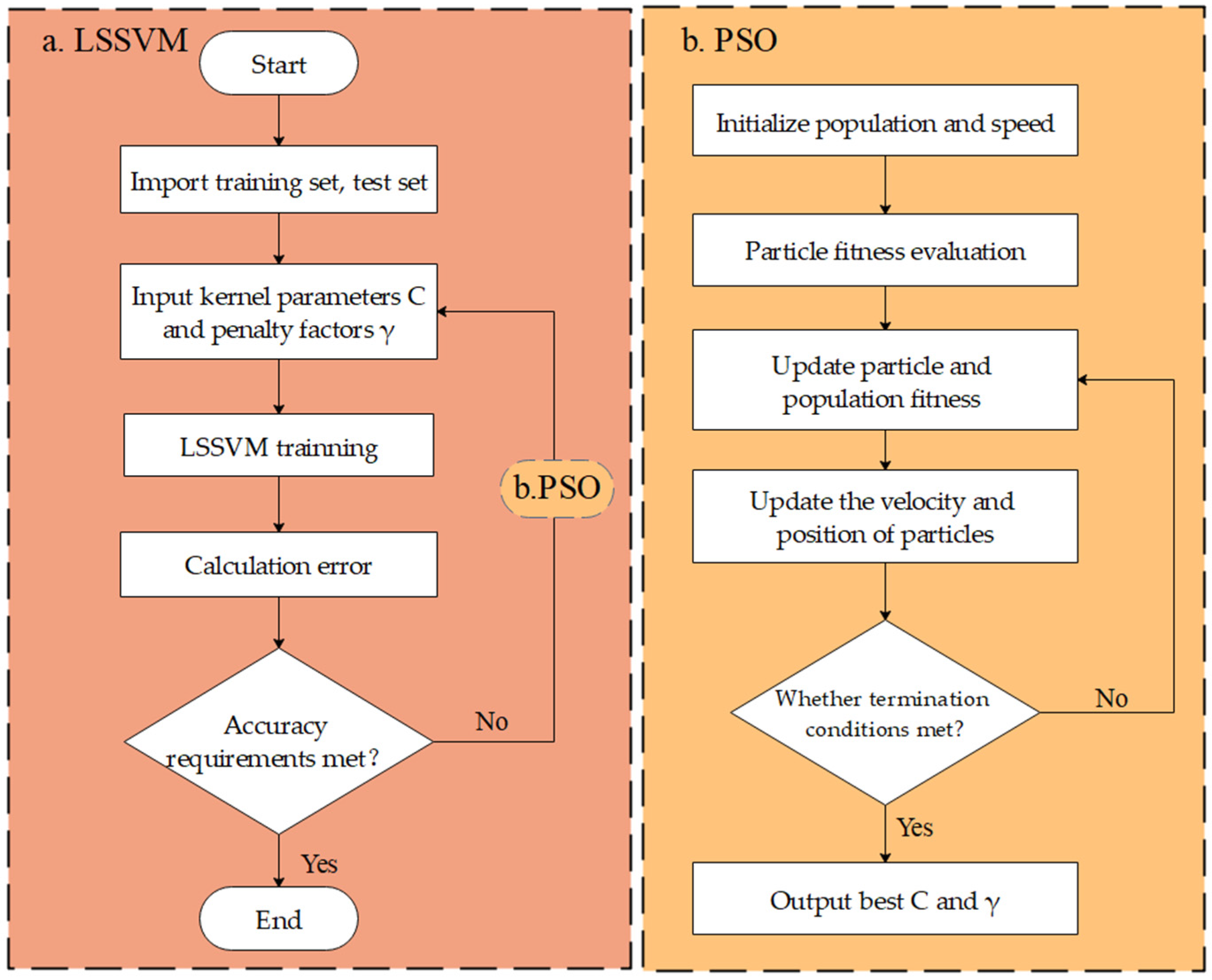
Figure 1 shows the overall process of the PSO-LSSVM algorithm. The kernel parameter C and penalty factor in the LSSVM play decisive roles in the accuracy of the model. Therefore, the PSO is utilized to optimize the C and the , and the process of the PSO algorithm is presented in Figure 1b. The specific steps are summarized:
- (a)
- Initialize parameters containing population size m, number of iterations , learning factor c, initial position , and initial velocity of the particles, etc.;
- (b)
- Predict learning samples by the particle vectors in the LSSVM. A prediction error of the current position of each particle is regarded as a fitness value of each particle. By comparing the current fitness value of each particle with its optimal fitness value, the current position is taken as the optimal position if the former is better than the latter;
- (c)
- Compare the adaptation value of each particle’s optimal position with the adaptation value of the population’s optimal position. If the former is better than the latter, this particle’s optimal position is replaced with the population’s optimal position;
- (d)
- Calculate an inertial weight and update the and of each particle by Equations (5) and (6);
- (e)
- Judge whether the maximum iteration is achieved or the accuracy requirement is satisfied. If any condition is reached, the procedure is ended and the optimal solution is found. Contrarily, step (b) will continue to be executed, and a new round of searches will be conducted.
2.5. Prediction Performance Measure
After training the prediction model, the predicted results are analysed using the coefficient of determination R2, Root Mean Square Error (RMSE), and Mean Absolute Error (MAE). R2 is the percentage of explainable variation to the total variation. A model with R2 of closely 1 means better performance results. The RMSE is used to reflect the deviation between the predicted value and the measured value. The MAE reflects the actual situation of the prediction error. The smaller the RMSE and the MAE, the higher the accuracy of the model. They are calculated as follows.
where is the measured value, is the predicted value, and represent their average values respectively, and N is the total number of samples.
3. Case Study
3.1. Geological Condition
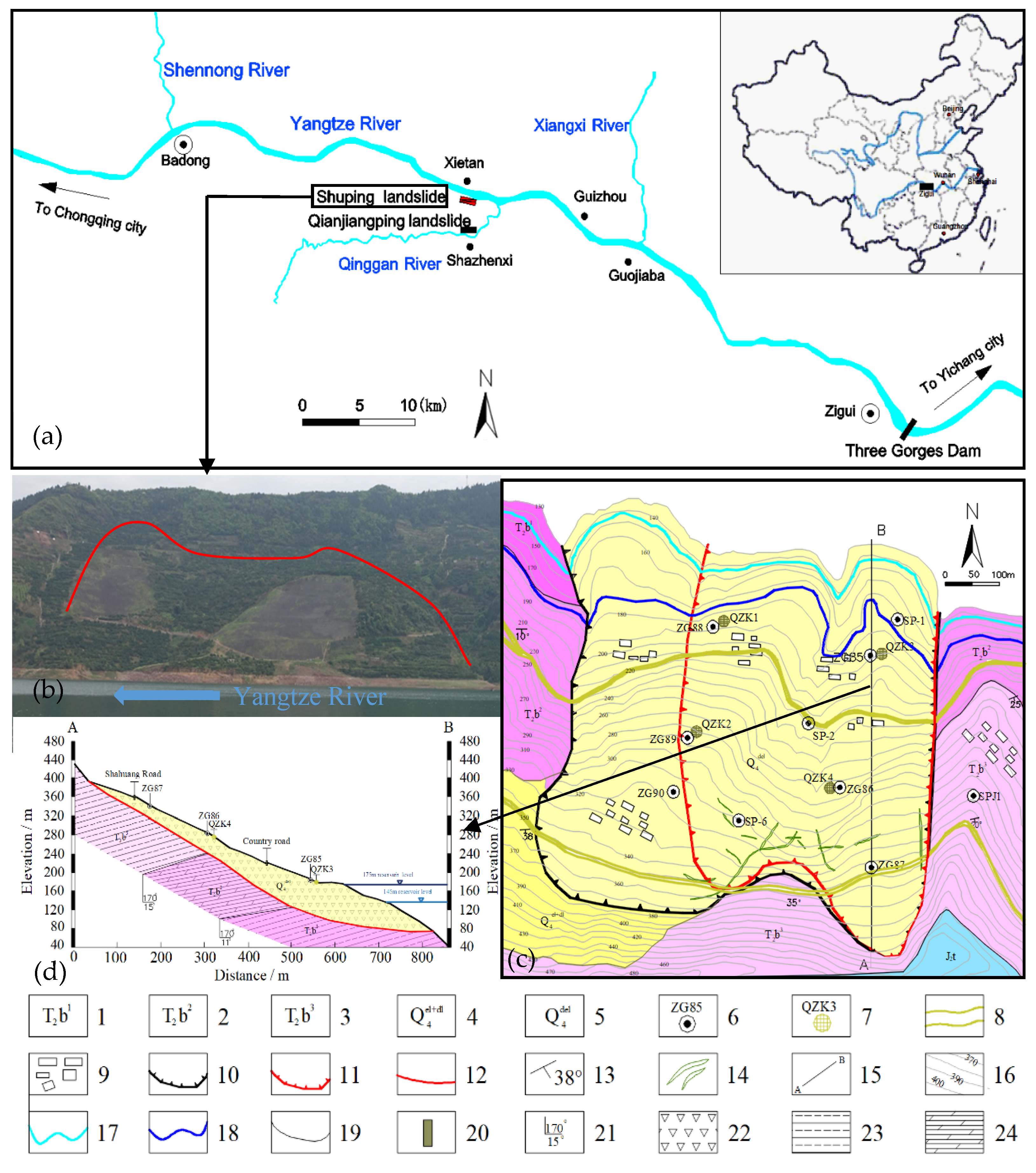
The Shuping Landslide is an unstable slope on the southern bank of the Yangtze River (Figure 2). The first level platform in this landslide is at 170 m elevation, and the second level platform is at 300 m elevation. Usually, the second level platform is a portion of the landslide back scarp. The overall spatial shape of the Shuping landslide is similar to an armchair, with gullies on both sides. The shear outlet elevation at the head scarp is about 70 m below the RWL. The landslide is approximately 800 m in length and 700 m in width. Shuping Landslide has a total area of approximately 55 × 104 m2, a thickness of 20–70 m, and a total volume of 2750 × 104 m3. The primary deformation region is in the center and east of the landslide, with the volume of approximately 1575 × 104 m3 [27].
The strata of the Shuping landslide area ranges from the first to third members of the Triassic Badong Formation (T2b1–3). The first section of the Badong Formation (T2b1) has light grey and grey-green marl interbedded with mudstone and shale, the second section (T2b2) has purple-red mudstone and argillaceous siltstone interbedded, and the third section (T2b3) has greyish brown and light grey argillaceous limestone [28,29].
According to a field geological investigation, the main component of the sliding zone the Shuping landslide is yellow-brown residual gravel soil with a particle size of 1–15 cm, and an angular or subangular shape. The landslide is divided into two main deformation regions, the east landslide region and the west landslide region. The sliding zone of the east landslide region is the contact strip between the accumulation layer and bedrock. The sliding soil of the landslide is mostly formed of yellow-brown, cyan-grey, or purple silty clay with sandstone, mudstone, and limestone gravel with a thickness of 0.6–1.0 m. In the west landslide zone, there is a two-layer sliding zone. The shallow sliding zone is developed in the slope deposit and is made up of yellowish-green silty clay, sandstone, or mudstone breccia with a thickness of 1.0–1.2 m. The deep sliding zone that is the contact strip between the accumulation layer and the bedrock zone has a thickness of 1.1–1.7 m, and is mostly made up of brown-yellow, purple-red silty clay, mudstone, or sand-mudstone breccia. The sliding bed is a typical sliding red-rock of the Triassic Badong Formation. In Figure 2d, the view of geologic profile is also displayed.
3.2. Deformation Characteristics
3.2.1. Ground Deformation Characteristics
The Shuping landslide is an ancient landslide, which has shifted the main sliding direction several times. Since the TGR began impounding in 2003, the landslide has been constantly deformed. Particularly, the landslide has suffered significant deformation during the period from May to August every year [30].
Since October 2003, the landslide deformation mainly occurred near the head scarp. In January 2004, obvious ground cracks occurred on the landslid. At the margin of the eastern part of the landslide, a shear crack with a length of about 100 m extends in the north-south direction. Large cracks that extend sporadically from east to west and progressively shift from NEE to NW may be seen along the Shahuang Road at the back scarp of the landslide. The total length of these cracks is over 400 m. Herein, the maximum length of a single crack exceeds 10 m. Furthermore, due to the generation of the cracks in their house walls, all native people have been relocated [31].
After April 2007, surface deformation phenomena have been observed increasingly. Transverse cracks have formed on the steep slope at the back scarp of the landslide and the Shahuang Road. These cracks have a width of 5–8 cm, length of 20–40 m, and depth of approximately 10–20 cm. Tensile cracks have started to appear at the back scarp on the western side of the landslide and are gradually moving in the direction of the northwest. The heavy rainfall damaged the stability of the landslide several times in August 2008. Numerous settlement cracks formed on the Shahuang Road at the border region of the eastern landslide zone, which caused the subgrade to collapse. At the same time, the cracks in this direction continue to grow downward along the east border of the landslide, with a total length of roughly 100 m and a width of 0.5–3 cm. Finally, a small-scale collapse has occurred continuously in the Shuping landslide.
The main deformation zone has basically formed since May 2009 due to the ongoing development of landslide deformation. At the west margin of the major deformation zone, a series of pinnate shear-tension cracks can be found, with considerable overall extension. The cracks usually sink by 20–50 cm, open by 2–20 cm, and strike at 300–360 degrees, crossing the road at the lower part of the slope to the gully. The original cracks in the main deformation zone are continuously extending. The deformation in the eastern part is dominated by closed shear cracks, while the deformation at the back scarp is dominated by tensile cracks.
In 2014, the deformation of the main deformation zone became more serious. For example, the initial cracks at the landslide boundary have gradually extended and expanded. The shear cracks at the east boundary and the tensile cracks at the back scarp boundary were further connected. Additionally, shear cracks and tension cracks on the west boundary of the landslide were distributed in the echelon, and most of them are connected. Therefore, in August 2014, some emergency measures were taken to improve the stability of the landslide.
3.2.2. Analysis of Test Data
Special monitoring methods to monitor deep displacement and surface displacement have been conducted in the Shuping landslide since June 2003, as shown in Figure 2.
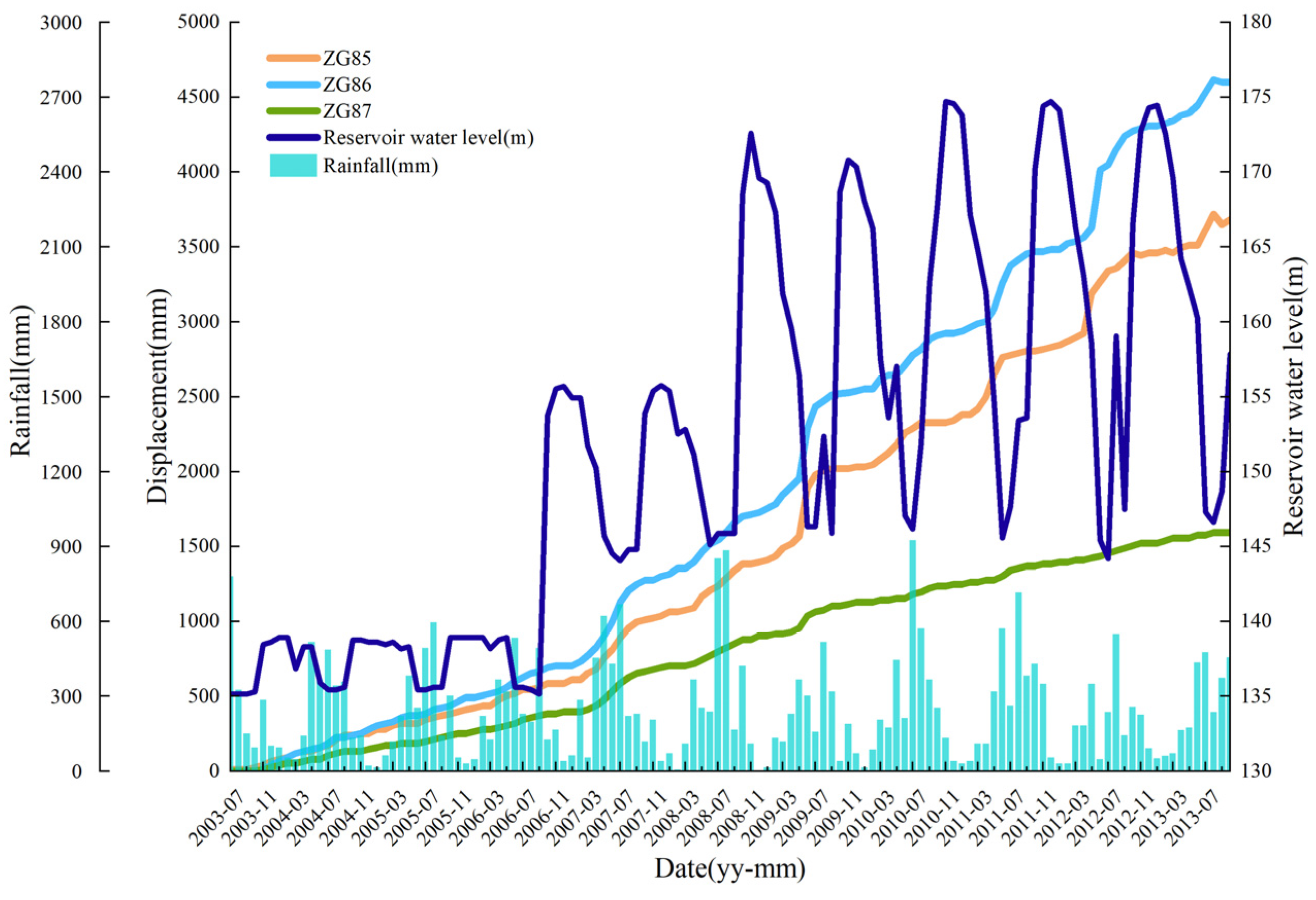
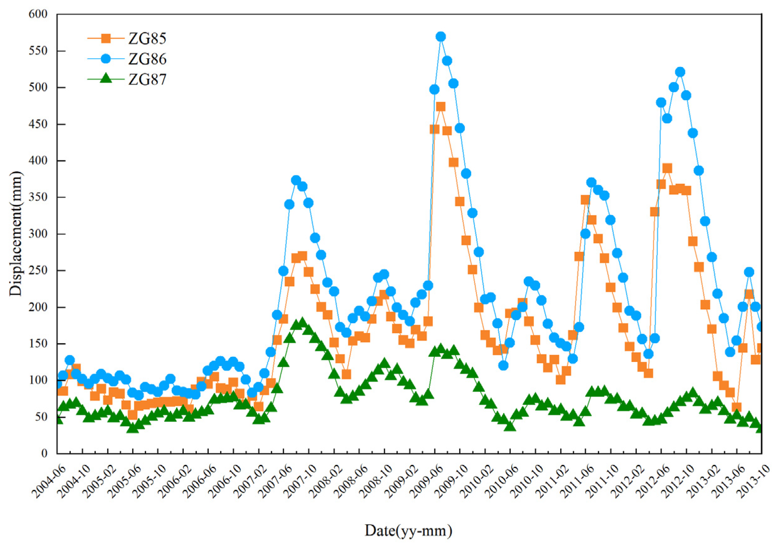
The ZG85, ZG86, ZG87 are located in the front, middle and rear of the landslide, so these three representative GPS stations are selected for analysis. Figure 3 depicts the CD of three monitoring stations at the Shuping landslide. The displacement of the Shuping landslide occurs mostly in the main deformation zone, and the displacement has typical step-type characteristics. The curves of ZG85 and ZG86 show a similar pattern, indicating that the landslide is deforming in a synchronized and step-type manner. The monitoring curve exhibits an obvious rising tendency every year from May to August, while keeping steady from October to April of the following year. In other words, the landslide displacement rises gradually in the summer every year. Notably, in 2007, 2009, 2011, and 2012, the displacement changes were evidently larger than in other years, in which the largest increment is in June and July.
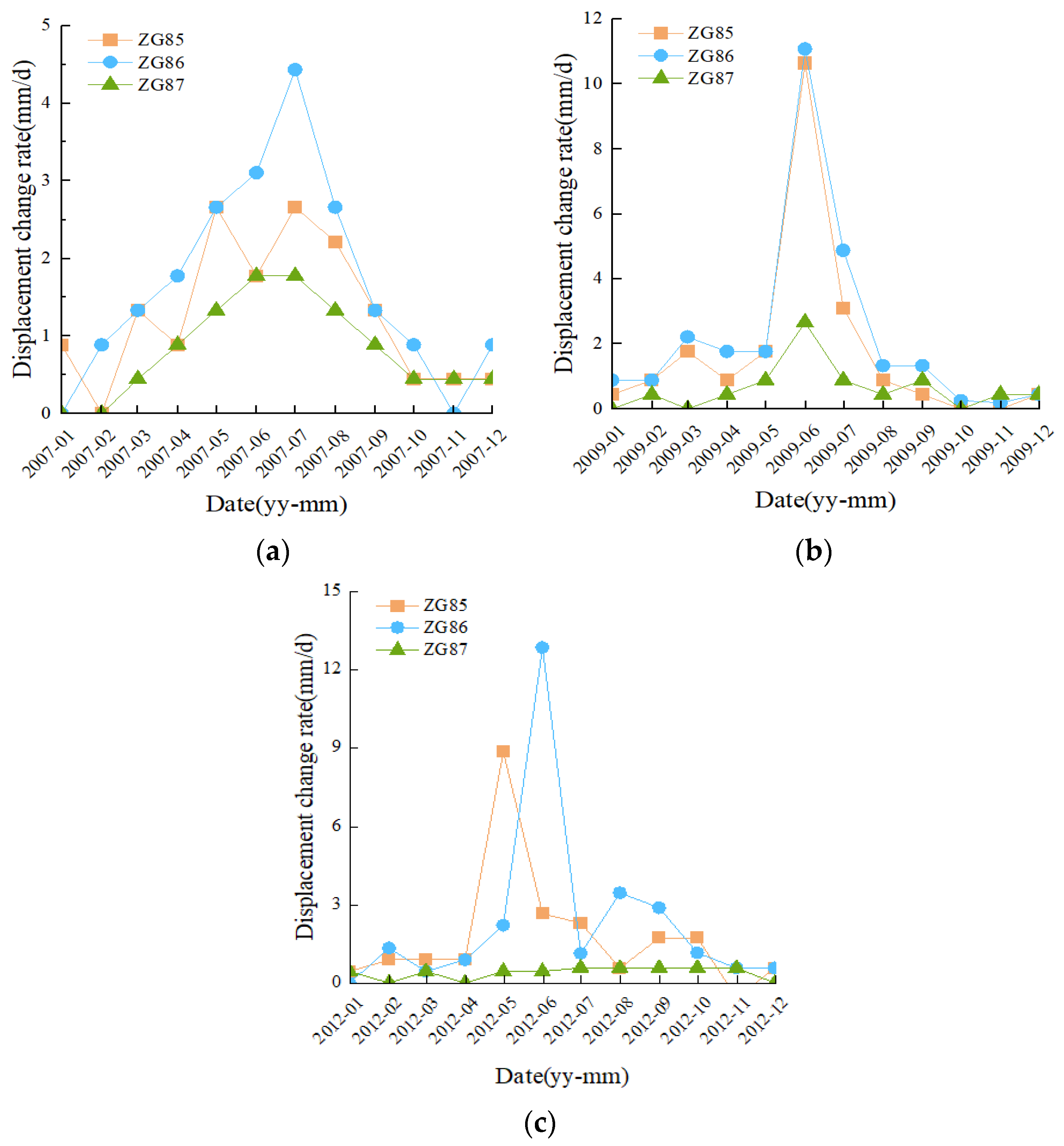
Figure 4 displays the daily displacement change rate in 2007, 2009, and 2012, and the curves of the three monitoring stations exhibit great fluctuation. In June and July each year, the daily displacement change rate of every monitoring station reaches the maximum, and the landslide occurs with serious deformation. Afterward, the daily displacement change rate progressively diminishes. For instance, the daily displacement change rate at monitoring station ZG86 exceeded 12.85 mm/d in June 2012, but was only about 2 mm/d in other months. The analysis reveals that the landslide deformation is characterized by the step-type and is affected by the rise and drop of the RWL and seasonal rainfall.
3.3. Triggering Factors Analysis
3.3.1. Foundation of Geological Factors
Landslides are possible on any slope with a gradient greater than 10°. The Shuping landslide is located on the Yangtze River’s south bank, with an average gradient of about 25 degrees. The landslide mass’s landform is a combination of steep and slow. The head scarp of the landslide is below the Yangtze River, and gullies have developed on both sides. Therefore, the landslide has a good free face. These unique topographic features provide an underpinning for the occurrence and progression of a landslide.
The Badong Formation, in which soft and hard rocks are interbedded, is the stratum of the Shuping landslide. A mudstone weak layer is easily worn and rich in montmorillonite, Ili stone, and other minerals. The weak layer gradually evolved into a sliding surface when it came into contact with water. Therefore, the slippery rock stratum in the landslide area serves as the structural foundation for the deformation of the landslide. In addition, under the action of gravity, the weak area at the bottom of the sliding body undergoes creep and pulls the upper rock and soil masses to produce tension deformation.
Furthermore, fissures regularly develop in the landslide area as a result of regional tectonic action, and their occurrences coincide with the landslide orientation, offering a free face for landslide development.
3.3.2. Effects of Reservoir Water Level and Rainfall
During the operation of the Three Gorges Dam, the RWL is adjusted with the seasons. The RWL ranges between 145 m and 175 m throughout a typical hydrological year. The RWL usually decreases to its lowest level of 145 m in the summer for flood control. In the dry season, the RWL maintains 175 m to enable electricity generation and shipping. Typically, the RWL reaches its lowest level in June and July and its highest level in October and November.
Figure 3 presents the relationships between the CD of the Shuping landslide with the rainfall and the RWL. Obviously, the sharp increase in landslide deformation often happens between May and August each year when the RWL is in a dropping stage or there is heavy rainfall. From October to March of the following year, the landslide displacement essentially stays flat. In the meantime, the RWL is in the high-level change stage with less rainfall. This demonstrates that the drop in the RWL and seasonal rainfall affected the displacement rate of the Shuping landslide. Moreover, the displacement of the landslide occurs after the decline of the RWL, characterized by a hysteresis effect.
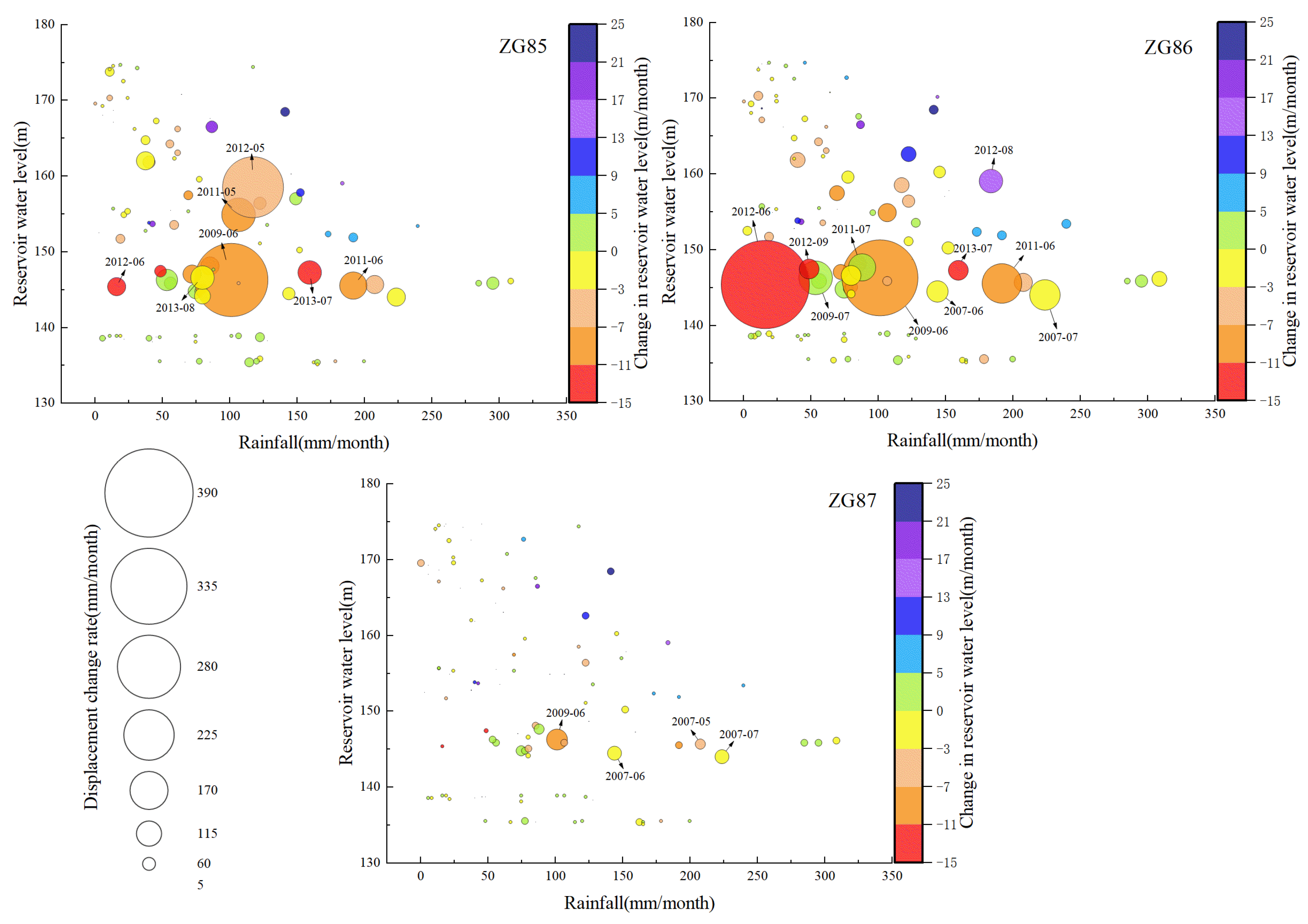
Figure 5 shows the relationships between the monthly displacement change rate of the landslide and the change in RWL, the rainfall more intuitively. The size of the bubbles represents the monthly displacement change rate. Big bubbles concentrate at the RWL of 145 m, while the range of the RWL changes from −3 to −11 m every month. The bubbles in ZG87 are overall smaller than those in ZG85 and ZG86. Besides, Figure 2c shows that ZG85 is at the head scarp of the landslide, ZG86 is at the midsection, and ZG87 is at the back scarp of the landslide. The displacement of the landslide at the back scarp is much smaller than that of the landslide at the head scarp, which means that the Shuping landslide is retrogressive.
The two largest bubbles in ZG85 are in June 2009 and May 2012, while in ZG86 they are in June 2012 and June 2009. This is consistent with the situation shown in Figure 4. Since the 175 m impounding of the TGR in October 2008, the RWL drops rapidly to prevent flooding from June to July every year. In the meantime, the displacement of the landslide is also relatively large. Especially in 2009 and 2012, the displacement of the landslide reaches 319 mm/month and 266 mm/month, respectively. The result indicates that the decline of the RWL has a greater impact on the landslide deformation.
However, the bubbles in the cold color system are smaller, which indicates that the rise of the RWL has little influence on the landslide displacement. On the other hand, large bubbles mostly occur above 100 mm of rainfall, which indicates that rainfall also influences the landslide displacement. However, the bubbles in areas of heavy rainfall are smaller than those in the warm color system, indicating that the impact of the rainfall on the landslide displacement is less than that of the drop of the RWL. In conclusion, the displacement of the Shuping landslide is affected by comprehensive factors.
The main component of the sliding body in the Shuping landslide is weakly permeable silty clay with gravel. When the RWL rises, water seeps into the sliding body. During this period, the RWL is higher than the groundwater level in the sliding body due to the slow permeation rate. Therefore, the landslide is not easy to deform due to the existence of the water pressure. When the RWL drops, the groundwater in the sliding body drains to the Yangtze River. As the permeability of the sliding body is poor, the dropping rate of the groundwater is much lower than that of the RWL. Therefore, the osmotic pressure is formed with the direction of pointing to the empty face of the reservoir, which is conducive to the landslide deformation. At the same time, most rock and soil masses are still saturated due to the drops of groundwater moving slowly through the sliding body, which increases the self-weight of the landslide body, and makes it easier for the landslide to slide. Similarly, the landslide deformation under this condition exhibits the hysteresis effect. The higher the RWL dropping rate, the more obvious the hysteresis effect and the greater the landslide deformation. Therefore, the deformation of the Shuping landslide is greatly affected by the drop in the RWL, so the Shuping landslide is a typical reservoir downward landslide.
Additionally, rainfall infiltration also raises the self-weight of the landslide, leading to the generation of pore seepage pressure. Under these conditions, the shear strength of the rock and soil mass decreases. As shown in Figure 3, the steep rise of the CD from 2007 to 2013 is the same as that of the strong rainfall period. Therefore, rainfall is also one of the important influencing factors in the displacement of the Shuping landslide.
4. Results
4.1. Training Process
In this study, the TSM is applied to decompose the landslide displacement into the TTD and the PTD. The PTD is predicted by the PSO-LSSVM model. Taking the monitoring stations ZG85, ZG86, and ZG87 as examples, the monitoring data from June 2004 to October 2011 is used as the training data, and the data from November 2011 to October 2013 is used as the prediction data.
Using Equation (4), the TTD of three monitoring stations is extracted. According to the TSM, the CD of the landslide is expressed as the sum of the TTD and the PTD. Therefore, the value of the PTD is obtained by subtracting the calculated TTD from the CD. The PTD of the monitoring stations is shown in Figure 6.
The accuracy of models is directly proportional to the influence factors. Therefore, the grey correlation analysis is utilized to evaluate the correlations between the displacement and influence factors. Based on the analysis in Section 3, the PTD of the landslide is mainly affected by rainfall and RWL. In addition, the correlation of the displacement changes in a single month, two months, three months, a half year, and one year are calculated to analyse the influence of different times on the increments in the PTD of the landslide according to the grey correlation analysis (Table 1). The value of ranges from [0, 1]. The larger the value, the higher the correlation between the two factors. Table 1 shows that the correlation of the increments on the PTD in a half year is the largest, so this factor is selected as the influence factor of the PTD.
According to the grey correlation analysis, the correlation degree between each influence factor and the PTD is calculated. Table 2 presents the correlations for each influence factor. The four influence factors are closely related to the PTD due to > 0.8, which affords a theoretical foundation for the accurate prediction of the model.
In summary, a total of five parameters, including rainfall over the previous month, rainfall over the previous two months, RWL, change in RWL over the previous month and period displacement over the previous half year, are picked as the input variables.
Following the selection of the influence factors, they are fed into the model for training. In this study, the PSO-LSSVM is used to predict the PTD, and the following are the specific operation steps:
- (a)
- Divide the data set. The PTD from June 2004 to October 2011 is considered as the training data, and the two years of data from November 2011 to September 2013 are considered as the prediction data;
- (b)
- Set the parameters in the PSO. Supposing that the penalty factor C is [0.1, 1000], the kernel parameter is [0.01, 1000], the number of the particle swarm is 20, the maximum number of iterations is 200, the learning factor = = 1.5, and the inertial weight ω = 0.5;
- (c)
- Determine the value of optimization parameters;
- (d)
- Train the LSSVM model. The optimal penalty factor C is installed as 229.12, and the kernel parameter is installed as 0.01 in the LSSVM, obtained by the optimization of the PSO. Afterward, the fitness value of the model is calculated by the optimal parameters.
4.2. Results and Analysis
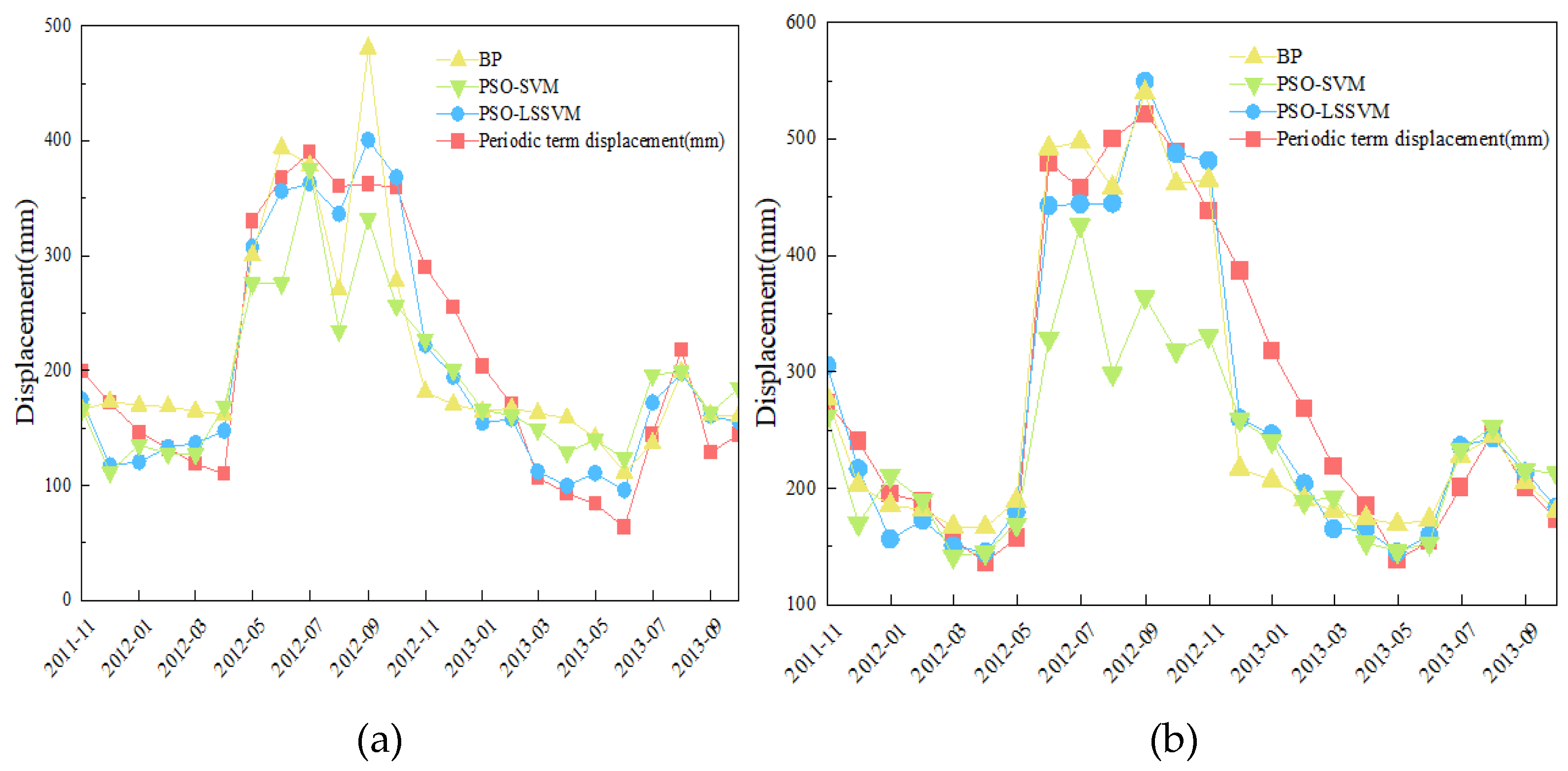
To contrast the applicability of the PSO-LSSVM model, the BP model and the PSO-SVM model are also constructed to predict the PTD of three monitoring stations of the Shuping landslide. The predicted results are shown in Figure 7, and Table 3 shows the error of each model.
In ZG85 (Figure 7a), the BP model has particularly large deviations from predicted results in August 2012 and September 2012. Therefore, the R2 of the BP model is the smallest of the three models. Except for individual points, both the BP model and the PSO-SVM model predicted results inferior to the PSO-LSSVM model at each point. For this reason, the MAE values and RMSE values of the PSO-LSSVM model are much smaller than the others. In ZG86 (Figure 7b), the PSO-SVM model had poor prediction from June 2012 to February 2013. Thus, the MAE and RMSE values of the model are exceptionally large. In ZG87 (Figure 7c), the predicted results of the PSO-SVM model are generally poor, and the predicted results of the BP model are better than those of the PSO-LSSVM model except for August 2012 and October 2012. Therefore, the R2 of the BP model is closer to 1, while that of the PSO-SVM model is the smallest. It means that the single prediction of the BP model is quite good. Overall, the PSO-LSSVM model shows good predicted results at the three monitoring stations, which means that the model is stable and accurate.
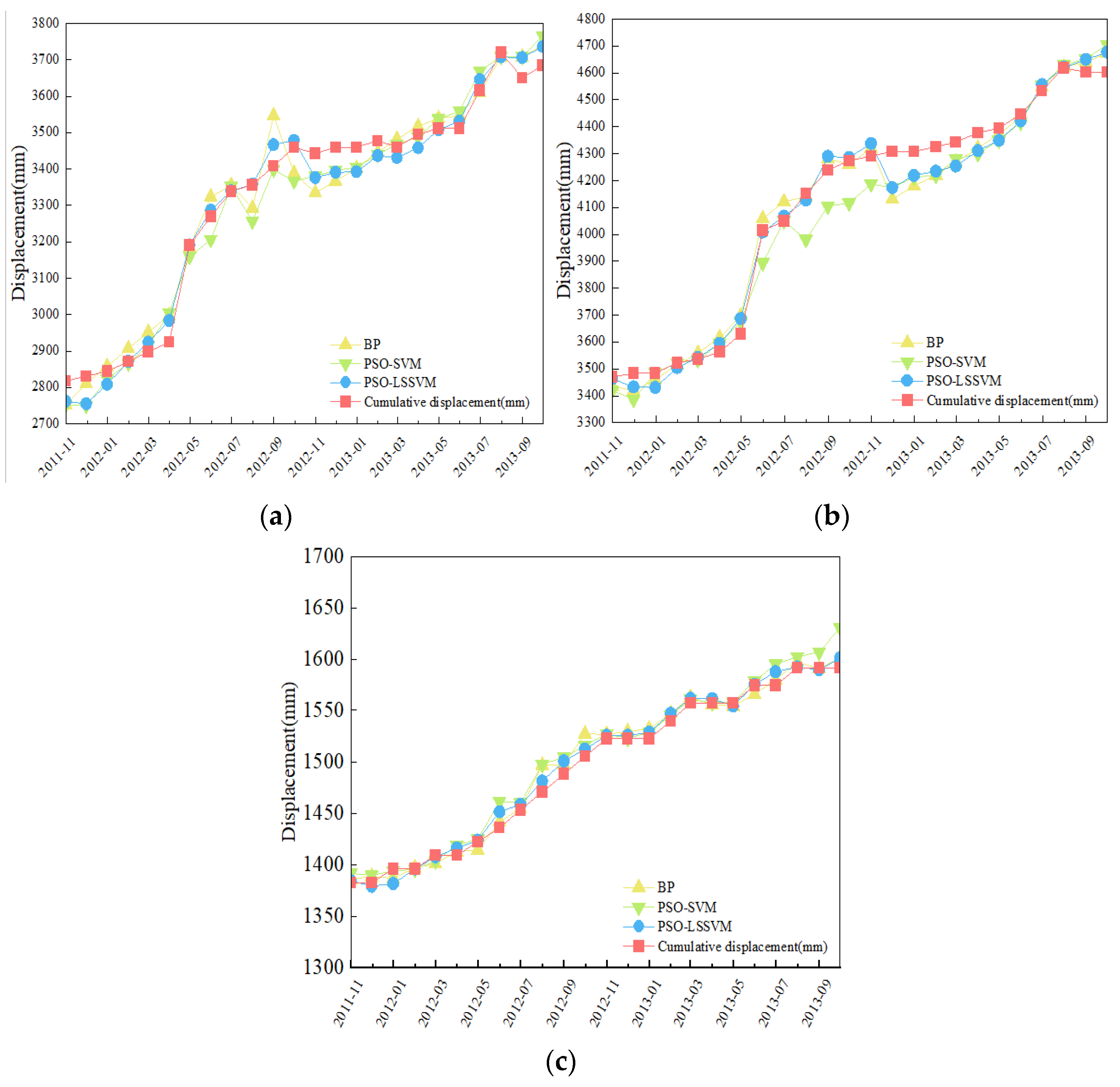
In addition, to further demonstrate the superiority of the model, we also need to predict TTD. Because the TTD approximates monotonous increment, a simple least squares method with a better effect can be used to fit it. The CD is fitted by adding the two prediction values according to the TSM. Figure 8 presents the CD predicted results, and Table 4 shows the error of the CD for each model.
The predicted results of each prediction model are quite different near the abrupt point of the CD in ZG85, as shown in Figure 8a. However, because the PSO-LSSVM model has the smallest deviation value, its predicted results are better than those of the BP model and the PSO-SVM model. Additionally, the prediction performance of the PSO-SVM in ZG86 is significantly lower than that of the other two prediction models. Three models show a good fit result in the landslide prediction of ZG87, which can be seen in Figure 8c. In total, in the PSO-LSSVM model, the R2 of three monitoring stations is larger than 0.98, and the RMSE values are the smallest among the three models. Thus, the PSO-LSSVM model has good accuracy in the landslide displacement prediction.
5. Discussion
As shown in Figure 3, the deformation of the Shuping landslide exhibits step-type characteristics when the surface monitoring data are analysed. Based on the monitoring data for ZG85, the deformation increases with time. The possible situation is that sliding might have occurred on the Shuping landslide if no treatments had been employed. Therefore, some emergency treatments, such as unloading, were conducted in 2014.
Water also affects landslide deformation. Since information on rainfall and RWL is easy to collect, it is often used for quantitative analysis of landslides. The displacement change rate of the Shuping landslide is more influenced by the decrease in RWL compared with rainfall, and it has an obvious lagging effect. Therefore, RWL scheduling needs to be planned in advance according to meteorological forecasts to avoid a faster rate of water level decline, which will cause damage to the slope.
The establishment of a landslide prediction model by machine learning is a hot research direction in landslide prediction. In addition to the selection of models, the selection of input variables is also important. The input of variables with high correlation is effective in improving the accuracy of the model. The results show that there is a significant difference in the correlation between the PTD and displacement with different time differences. As a result, it is critical to investigate the factors that influence landslide deformation in its early stages.
To prove the predictive effect of the PSO-LSSVM model, the BP model and the PSO-SVM model were established under the same conditions. The results of displacement prediction in Section 4 show that the PSO-LSSVM model has the best prediction effect because of the minimum deviation of the predicted value at the point of trend break. The BP model is easy to fall into a local minimum by the gradient descent method, so it is hard to find the global optimal solution, which causes large errors in some prediction points. Furthermore, the old sample in the BP algorithm will be forgotten after learning the new sample, which leads to a large span between adjacent predictions during the model training (Figure 7a). The SVM model is sparse, so it can sort the data well and has strong stability. However, the SVM model has a higher Lagrange multiplier dependence, which is difficult to find, so the fitting accuracy of the PSO-SVM model is not good. The LSSVM model not only inherits the advantages of the SVM model, but also improves the calculation of Lagrange multipliers, which makes the model more accurate. Therefore, among the three models, the PSO-LSSVM model has both accuracy and stability and can provide reliable reference materials for landslide prediction.
6. Conclusions
The Shuping landslide is an ancient landslide, characterized by constant deformation. The landslide displacement changes with time into a step-type shape. Combined with the rainfall and the RWL, the deformation of the landslide is strongly influenced by heavy rainfall and the decline of the RWL, characterized by a typical hysteresis effect.
According to the TSM, the CD of the landslide is decomposed into the PTD and the TTD. The PSO-LSSVM model is established to predict the PTD of the landslide by selecting five input variables using the grey correlation analysis, including rainfall over the previous month, rainfall over the previous two months, the RWL, change in RWL over the previous month and period displacement over the previous half year. Additionally, the TTD was predicted using a least squares model. The rationality of the PSO-LSSVM model is verified by contrasting it with the BP model and the PSO-SVM model based on R2, MAE, and RMSE. In the CD predicted results, the R2 of the PSO-LSSVM model in three monitoring stations is larger than 0.98, and the MAE values and the RMSE values are the smallest among the three models. The results reveal that the PSO-LSSVM model has good accuracy and has a certain application value in landslide prediction.
Author Contributions
Methodology, W.J.; software, W.J. and D.L.; validation, W.J. and T.W.; formal analysis, W.J.; investigation, W.J. and W.G.; resources, T.W.; data curation, W.J., Z.Q., Y.W. and D.H.; writing—original draft preparation, W.J.; writing—review and editing, W.J. and T.W.; visualization, W.J.; supervision, M.H.; project administration, T.W. All authors have read and agreed to the published version of the manuscript.
Funding
The work was funded by the National Natural Science Foundation of China (No. 42002268); Science and technology program of Tibet Autonomous Region (XZ202202YD0007C); Open Fund of Badong National Observation and Research Station of Geohazards (No. BNORSG-202204).
Data Availability Statement
The data that support the findings of this study are available on request from the corresponding author upon reasonable request.
Conflicts of Interest
The authors declare no conflict of interest.
References
- Su, Z.; Wang, Y.; Zhang, H. Study on the Failure Mechanism, Safety Grading and Rainfall Threshold of Landslide Caused by Typhoon Rainstorm. Geotech. Geol. Eng. 2022, 40, 2201–2211. [Google Scholar] [CrossRef]
- Tang, H.; Wasowski, J.; Juang, C.H. Geohazards in the three Gorges Reservoir Area, China–Lessons learned from decades of research. Eng. Geol. 2019, 261, 105267. [Google Scholar] [CrossRef]
- Li, C.; Fu, Z.; Wang, Y.; Tang, H.; Yan, J.; Gong, W.; Yao, W.; Criss, R.E. Susceptibility of reservoir-induced landslides and strategies for increasing the slope stability in the Three Gorges Reservoir Area: Zigui Basin as an example. Eng. Geol. 2019, 261, 105279. [Google Scholar] [CrossRef]
- Ren, F.; Wu, X.; Zhang, K.; Niu, R. Application of wavelet analysis and a particle swarm-optimized support vector machine to predict the displacement of the Shuping landslide in the Three Gorges, China. Environ. Earth Sci. 2015, 73, 4791–4804. [Google Scholar] [CrossRef]
- Huang, F.; Yin, K.; Zhang, G.; Gui, L.; Yang, B.; Liu, L. Landslide displacement prediction using discrete wavelet transform and extreme learning machine based on chaos theory. Environ. Earth Sci. 2016, 75, 1376. [Google Scholar] [CrossRef]
- Huang, F.; Huang, J.; Jiang, S.; Zhou, C. Landslide displacement prediction based on multivariate chaotic model and extreme learning machine. Eng. Geol. 2017, 218, 173–186. [Google Scholar] [CrossRef]
- Lian, C.; Zeng, Z.; Yao, W.; Tang, H. Ensemble of extreme learning machine for landslide displacement prediction based on time series analysis. Neural Comput. Appl. 2014, 24, 99–107. [Google Scholar] [CrossRef]
- Goh, A.T.C. Back-propagation neural networks for modeling complex systems. Artif. Intell. Eng. 1995, 9, 143–151. [Google Scholar] [CrossRef]
- Zhu, X.; Ma, S.; Xu, Q.; Liu, W. A WD-GA-LSSVM model for rainfall-triggered landslide displacement prediction. J. Mt. Sci. 2018, 15, 156–166. [Google Scholar] [CrossRef]
- Fang, K.; Tang, H.; Li, C.; Su, X.; An, P.; Sun, S. Centrifuge modelling of landslides and landslide hazard mitigation: A review. Geosci. Front. 2023, 14, 101493. [Google Scholar] [CrossRef]
- Meyer, D.; Leisch, F.; Hornik, K. The support vector machine under test. Neurocomputing 2003, 55, 169–186. [Google Scholar] [CrossRef]
- Han, H.; Shi, B.; Zhang, L. Prediction of landslide sharp increase displacement by SVM with considering hysteresis of groundwater change. Eng. Geol. 2021, 280, 105876. [Google Scholar] [CrossRef]
- Ma, J.; Wang, Y.; Niu, X.; Jiang, S.; Liu, Z. A comparative study of mutual information-based input variable selection strategies for the displacement prediction of seepage-driven landslides using optimized support vector regression. Stoch. Environ. Res. Risk Assess. 2022, 36, 3109–3129. [Google Scholar] [CrossRef]
- Wang, Y.; Tang, H.; Huang, J.; Wen, T.; Ma, J.; Zhang, J. A comparative study of different machine learning methods for reservoir landslide displacement prediction. Eng. Geol. 2022, 298, 106544. [Google Scholar] [CrossRef]
- Zhang, Y.; Chen, X.; Liao, R.; Wan, J.; He, Z.; Zhao, Z.; Zhang, Y.; Su, Z. Research on displacement prediction of step-type landslide under the influence of various environmental factors based on intelligent WCA-ELM in the Three Gorges Reservoir area. Nat. Hazards 2021, 107, 1709–1729. [Google Scholar] [CrossRef]
- Wen, T.; Tang, H.M.; Wang, Y.K.; Lin, C.Y.; Xiong, C.R. Landslide displacement prediction using the GA-LSSVM model and time series analysis: A case study of Three Gorges Reservoir, China. Nat. Hazards Earth Syst. Sci. 2017, 17, 2181–2198. [Google Scholar] [CrossRef]
- Zhang, Y.; Tang, J.; He, Z.; Tan, J.; Li, C. A novel displacement prediction method using gated recurrent unit model with time series analysis in the Erdaohe landslide. Nat. Hazards 2021, 105, 783–813. [Google Scholar] [CrossRef]
- Gao, W.; Dai, S.; Chen, X. Landslide prediction based on a combination intelligent method using the GM and ENN: Two cases of landslides in the Three Gorges Reservoir, China. Landslides 2020, 17, 111–126. [Google Scholar] [CrossRef]
- Li, S.; Wu, N. A new grey prediction model and its application in landslide displacement prediction. Chaos Solitons Fractals 2021, 147, 110969. [Google Scholar] [CrossRef]
- Zhang, Y.; Tang, J.; Liao, R.; Zhang, M.; Zhang, Y.; Wang, X.; Su, Z. Application of an enhanced BP neural network model with water cycle algorithm on landslide prediction. Stoch. Environ. Res. Risk Assess. 2021, 35, 1273–1291. [Google Scholar] [CrossRef]
- Hecht-Nielsen; Robert. Theory of the backpropagation neural network. Neural Netw. 1988, 1, 445. [Google Scholar] [CrossRef]
- Zeng, J.; Tan, Z.H.; Matsunaga, T.; Shirai, T. Generalization of Parameter Selection of SVM and LS-SVM for Regression. Mach. Learn. Knowl. Extr. 2019, 1, 745–755. [Google Scholar] [CrossRef]
- Zhou, C.; Yin, K.; Cao, Y.; Intrieri, E.; Ahmed, B.; Catani, F. Displacement prediction of step-like landslide by applying a novel kernel extreme learning machine method. Landslides 2018, 15, 2211–2225. [Google Scholar] [CrossRef]
- Deng, W.; Yao, R.; Zhao, H.; Yang, X.; Li, G. A novel intelligent diagnosis method using optimal LS-SVM with improved PSO algorithm. Soft Comput. 2019, 23, 2445–2462. [Google Scholar] [CrossRef]
- Miao, F.; Wu, Y.; Xie, Y.; Li, Y. Prediction of landslide displacement with step-like behavior based on multialgorithm optimization and a support vector regression model. Landslides 2018, 15, 475–488. [Google Scholar] [CrossRef]
- Cai, Z.; Xu, W.; Meng, Y.; Shi, C.; Wang, R. Prediction of landslide displacement based on GA-LSSVM with multiple factors. Bull. Eng. Geol. Environ. 2016, 75, 637–646. [Google Scholar] [CrossRef]
- Wang, F.; Zhang, Y.; Huo, Z.; Peng, X.; Araiba, K.; Wang, G. Movement of the Shuping landslide in the first four years after the initial impoundment of the Three Gorges Dam Reservoir, China. Landslides 2008, 5, 321–329. [Google Scholar] [CrossRef]
- Wu, Q.; Tang, H.; Ma, X.; Wu, Y.; Hu, X.; Wang, L.; Criss, R.; Yuan, Y.; Xu, Y. Identification of movement characteristics and causal factors of the Shuping landslide based on monitored displacements. Bull. Eng. Geol. Environ. 2019, 78, 2093–2106. [Google Scholar] [CrossRef]
- Wen, T.; Tang, H.; Huang, L.; Wang, Y.; Ma, J. Energy evolution: A new perspective on the failure mechanism of purplish-red mudstones from the Three Gorges Reservoir area, China. Eng. Geol. 2020, 264, 105350. [Google Scholar] [CrossRef]
- Huang, D.; Gu, D.M.; Song, Y.X.; Cen, D.F.; Zeng, B. Towards a complete understanding of the triggering mechanism of a large reactivated landslide in the Three Gorges Reservoir. Eng. Geol. 2018, 238, 36–51. [Google Scholar] [CrossRef]
- Wu, Q.; Xu, Y.; Tang, H.; Fang, K.; Jiang, Y.; Liu, C.; Wang, L.; Wang, X.; Kang, J. Investigation on the shear properties of discontinuities at the interface between different rock types in the Badong formation, China. Eng. Geol. 2018, 245, 280–291. [Google Scholar] [CrossRef]
Figure 1.
The flow chart of the combination algorithm.

Figure 2.
Basic information of Shuping landslide. (a) Location of the Shuping landslide, modified from [31]. (b) Photo of the Shuping landslide. (c) Topographic map of the Shuping landslide displayed at the monitoring stations. (d) Geologic profile of section A–B. Note: 1, Siltstone mixed with mudstone and shale in T2b1; 2, Limestone and marble in T2b2; 3, Mudstone and siltstone in T2b3; 4, Quaternary residual slope deposits; 5, Quaternary landslide deposits; 6, Ground surface GPS monitoring stations and numbers; 7, Deep inclinometer hole and its number; 8, Road; 9, Buildings; 10, Landslide boundary; 11, Landslide boundary of main sliding area; 12, Sliding belt; 13, Rock occurrence; 14, Long ground fissures; 15, Sectional line; 16, Contour elevation; 17, The lowest RWL line; 18, the highest RWL line; 19, Stratum boundary; 20, Road in section; 21, Formation occurrence; 22, Quaternary landslide deposits; 23, Silty mudstone; 24, Argillaceous limestone.

Figure 3.
The correlation of the CD, rainfall and RWL with time.

Figure 4.
Daily displacement change rate at each monitoring station: (a) 2007; (b) 2009; (c) 2012.

Figure 5.
Correlation of monthly displacement change rate at each monitoring station with the RWL, rainfall, and the change in the RWL.
Figure 5.
Correlation of monthly displacement change rate at each monitoring station with the RWL, rainfall, and the change in the RWL.

Figure 6.
Extracted value of the PTD of each monitoring station.

Figure 7.
The PTD predicted result: (a) ZG85; (b) ZG86; (c) ZG87.


Figure 8.
The CD predicted results: (a) ZG85; (b) ZG86; (c) ZG87.


Table 1.
Correlation of displacement change at different times with the PTD of each monitoring station.
Table 1.
Correlation of displacement change at different times with the PTD of each monitoring station.
| Correlation ( ) | ZG85 | ZG86 | ZG87 |
|---|---|---|---|
| Period displacement over previous month | 0.855 | 0.842 | 0.822 |
| Period displacement over two previous months | 0.871 | 0.863 | 0.836 |
| Period displacement over three previous months | 0.844 | 0.882 | 0.849 |
| Period displacement over previous half year | 0.921 | 0.931 | 0.890 |
| Period displacement over previous year | 0.788 | 0.804 | 0.899 |
Table 2.
Correlation of the influence factor with the period term of each monitoring station.
| Correlation ( ) | ZG85 | ZG86 | ZG87 |
|---|---|---|---|
| Rainfall over previous month | 0.849 | 0.843 | 0.862 |
| Rainfall over previous two months | 0.845 | 0.861 | 0.866 |
| RWL | 0.851 | 0.818 | 0.808 |
| Change in RWL over previous month | 0.837 | 0.852 | 0.844 |
Table 3.
The error of the PTD of each model.
| Model | BP | PSO-SVM | PSO-LSSVM | |
|---|---|---|---|---|
| R2 | ZG85 | 0.7157 | 0.7955 | 0.9095 |
| ZG86 | 0.8631 | 0.8079 | 0.9091 | |
| ZG87 | 0.8047 | 0.4813 | 0.7727 | |
| MAE | ZG85 | 45.3365 | 45.8643 | 26.9320 |
| ZG86 | 33.1825 | 58.2599 | 30.7913 | |
| ZG87 | 6.4461 | 9.6564 | 5.5371 | |
| RMSE | ZG85 | 55.3498 | 54.5718 | 31.9132 |
| ZG86 | 49.8766 | 83.9435 | 41.6055 | |
| ZG87 | 8.4063 | 13.1436 | 7.2638 | |
Table 4.
The error of the CD of each model.
| Model | BP | PSO-SVM | PSO-LSSVM | |
|---|---|---|---|---|
| R2 | ZG85 | 0.9607 | 0.9718 | 0.9810 |
| ZG86 | 0.9753 | 0.9680 | 0.9823 | |
| ZG87 | 0.9875 | 0.9834 | 0.9932 | |
| MAE | ZG85 | 47.5004 | 45.4348 | 34.6488 |
| ZG86 | 49.5306 | 69.0451 | 44.5890 | |
| ZG87 | 7.2304 | 9.7076 | 5.7296 | |
| RMSE | ZG85 | 57.8430 | 54.1392 | 42.4378 |
| ZG86 | 64.1690 | 86.0639 | 55.4179 | |
| ZG87 | 9.2874 | 13.6112 | 7.3380 | |
Disclaimer/Publisher’s Note: The statements, opinions and data contained in all publications are solely those of the individual author(s) and contributor(s) and not of MDPI and/or the editor(s). MDPI and/or the editor(s) disclaim responsibility for any injury to people or property resulting from any ideas, methods, instructions or products referred to in the content. |
© 2023 by the authors. Licensee MDPI, Basel, Switzerland. This article is an open access article distributed under the terms and conditions of the Creative Commons Attribution (CC BY) license (https://creativecommons.org/licenses/by/4.0/).
Share and Cite
MDPI and ACS Style
Jia, W.; Wen, T.; Li, D.; Guo, W.; Quan, Z.; Wang, Y.; Huang, D.; Hu, M. Landslide Displacement Prediction of Shuping Landslide Combining PSO and LSSVM Model. Water 2023, 15, 612. https://doi.org/10.3390/w15040612
AMA Style
Jia W, Wen T, Li D, Guo W, Quan Z, Wang Y, Huang D, Hu M. Landslide Displacement Prediction of Shuping Landslide Combining PSO and LSSVM Model. Water. 2023; 15(4):612. https://doi.org/10.3390/w15040612
Chicago/Turabian StyleJia, Wenjun, Tao Wen, Decheng Li, Wei Guo, Zhi Quan, Yihui Wang, Dexin Huang, and Mingyi Hu. 2023. "Landslide Displacement Prediction of Shuping Landslide Combining PSO and LSSVM Model" Water 15, no. 4: 612. https://doi.org/10.3390/w15040612
Note that from the first issue of 2016, this journal uses article numbers instead of page numbers. See further details here.