Patterns in the Course of Gas Production Rates in Anaerobic Digestion—Prediction of Gas Production Rates Based on Deconvolution and Linear Regression

Abstract

Anaerobic digestion, including the gas storage and the CHP unit plays a key role in energy management of water ressource recovery facilities (WRRF). By demand-driven feeding management, a higher degree of utilization of the gas storage tanks can be achieved, which means that a greater decoupling of energy demand and energy generation is taking place. In this context, the predictability of the produced gas volume plays an important role. In this study, a concept was suggested to forecast gas production rates without the need for any analytical substrate characterization. Substrates lead to specific patterns in the course of the gas production rates, which can be fitted using Gaussian functions. As the parameters describing the Gaussian functions have a good correlation to the amount of substrate fed to the digester a prediction of the rates is possible. Within this study a coefficient of determination 82.9% over a period of 5 days was achieved.

1. Introduction

Above all, the sewage sludge treatment with the combined heat and power plants (CHP) offers good opportunities to decouple energy consumption and energy production on water resource recovery facilities (WRRF), especially since the effects on the wastewater treatment processes within the WRRF remains largely unaffected. The degree of flexible operation, i.e., the ability to generate a certain amount of electricity at a certain point in time, is directly related to the size and flexibility of the CHP units, the available gas storage capacity and the gas production rate. In order to make the interaction of substrate storage, digestion, gas storage and CHP as efficient as possible, all processes must be projectable. In other words, the following points must be known at all times:

• available amount and type of substrate
• gas production rates
• current gas storage capacities
• gas utility rate

In this context, the prediction of the produced gas volume plays a key role. In the past, numerous models for forecasting biogas quantities have been developed. These can be divided into static and dynamic models as well as deterministic and empirical models. Many models and equations are available to calculate produced gas volumes based on VSS, COD or carbon content or stoichiometric approaches e.g., Buswell Equation [1]. Using the theoretical conversion factor of 0.35 NLCH${}_4$/g COD the theoretical maximum gas volume can be calculated knowing the COD content of the substrate [2]. However, these approaches do not incorporate the dynamic characteristics of the anaerobic process. Deterministic models describe mathematically the underlying chemical, physical and biological processes. They are based on abstracting reality by defining only the essential process steps within a causality. Processes that do exist in reality, but are of secondary importance for the cause-effect relationship, are neglected. Thus a simplification of reality is created. In anaerobic degradation, the individual process steps are usually linked by a chain of zero-, first- and second-order kinetics. An overview of developed deterministic models is given in [3,4]. With the Anaerobic Digestion Model 1 (ADM1) [5] a mature deterministic dynamic model is available, able to describe the anaerobic processes in detail, allowing predictions on biogas volumes and conclusions on process stability. For this reason, the ADM1 was used in numerous works as the basis for control mechanisms [6,7]. Due to the high level of analytical work involved, the ADM1 in particular has only prevailed in the academic and planning environment. The original ADM1 defines 19 processes and requires the analysis of 64 parameters in order to characterize the input substrate and digester state. In addition, various constants have to be determined to characterize process kinetics, sometimes in a time-consuming manner, using a Biomethane potential tests (BMP) among others. Weinrich succeeded in systematically simplifying ADM1. He reduced the model to 4 process steps that were only described with first-order kinetics [8]. Lafratta introduced a model which is based only on 3 sequential first-order reactions and reduced necessary analysis of the substrate to the parameter VS, VFA, and acetic acid concentration [3]. While there are other models which require a smaller amount of analytical work (e.g., [3,8,9]), still chemical analysis remains a limiting factor, especially taking into account the changing substrate characteristics. The implementation of the ADM1 with the intention of actively controlling the digester is currently unknown. In his thesis, Maucky [7] presented a model predicted controller (MPC) based on the adapted ADM1 model according to Weinrich [8]. Continuously certain parameters of the model are optimized based on continuously measured data. As the descriptive function of the model is lost and the model parameters are solely optimized with regard to gas production, the question arises as to whether significantly simpler methods without a descriptive character do lead to the same results, so that the prediction is possible without complex chemical analysis and calibration.

Empirical models do not incorporate mathematical equations which derive from physical, chemical and biological processes but from analysis of time series data [10]. Computational intelligence and machine learning in particular had a major impact on empirical modeling. Recently many approaches based on Artificial Intelligence like neural networks (NN) were published [11,12,13]. An overview of different approaches is given in [14]. Jeong [11] presented a hybrid deep-learning architecture for forecasting biogas production. In the model, 17 input parameters of a large-scale plant, including inflows, SRT, mass loadings of BOD, COD, suspended solids, total nitrogen and total phosphorous among others, were taken into account. NN is known to depend on huge amounts of data to provide satisfying results [14]. However, in large-scale facilities the amount of data e.g., characterization of input sludges and co-substrates are limited and TS, COD or others are rarely measured on a daily basis. Continuously measuring sensors that could support the implementation of NN are not yet available. Due to the above mentioned limitations, there is a need for models that can be used for feeding control without significant additional effort in the operation of digesters to forecast the gas volume in an hourly resolution and thus can contribute to an efficient feeding management. Dittmer provided a linear regression model to predict gas production rates as a function of the amount of substrate. The influence of previous substrate additions is taken into account in the regression model, based on a cross-correlation analysis [15]. This model does not require any analytical effort.

As part of this work, an empirical method is presented in which past gas production curves are deconvoluted and a prognosis of future gas production rates are predicted using simple linear regression. The method also does not require any chemical analyses.

The numerous constituents of the substrates used in anaerobic digestion are subject to individual biological degradation processes, which are characterized by different conversion rates. Gallert and Winter [16] are illustrating the generalized metabolic pathways of proteins, carbohydrates and lipids. Within anaerobic systems, it could be shown that hydrolysis in particular is assumed to be the limiting process step [17,18]. Hydrolysis involves the solubilization of undissolved particulate matter and the biological decomposition of complex polymers into dimers and monomers using enzymes. Lipids are degraded to fatty acids, proteins to amino acids and carbohydrates into simple sugars. In anaerobic systems, hydrolysis is often mathematically described by first-order kinetic model [4]. Figure 1 shows hydrolytic constants $\left[d^{-1}\right]$ determined by Christ et al. [19] (at 55 °C), O’Rourke (1968) and Garcia-Heras (2003) for carbohydrates, proteins and lipids. The differences of the $k_{hyd}$-values indicate the different degradation velocities between these substrate groups.

All authors show differences between the three fractions with regard to the mean and the range of the $k_{hyd}$-values. It is reasonable to assume for a mixture that there is a time dependency between a constituent and its relative share on the amount of methane produced on the time axis. Depending on the constituents of the substrate specific patterns in the course of gas production rate should be observed. From numerous works, e.g., Hubert et al. 2019 a. o. it is known that the gas production rate follows a certain pattern after feeding organic substrates. With regard to raw sludge (mixture of primary and excess sludge), a very pronounced peak approx. 0.5–2 h after substrate addition is followed by a broad shoulder [24]. Depending on the organic load the production rate reaches an almost steady state after several hours. In addition, depending on the substrate used and the conditions in the reactor including chemical, biological and physical properties, further peaks and peak shoulders could be observed. In the present study it was investigated if the course of gas production rate can be described mathematically and thus allowing a statement about the future gas production rates without a characterization of the input substrate. In fact the identification of specific patterns could potentially give a feedback on the quantitative composition of the substrate as well as on the digester status. Although the latter is not part of the present study, it will be determined in further studies.

2. Materials and Methods

2.1. Reactor Setup

A semi-continuously fed reactor with a working volume of 15 L was used for the investigations. The reactor was fed one to two times a day with varying amounts of sludge. Digested sludge was removed from the reactor daily. The operating temperature was set to 37 ${}^{\circ }\mathrm{C}$. Hydraulic retention time was 15 days. The reactor was stirred continuously. The substrate consisted of a mixture of primary and secondary sludge in a ratio of 1:1. The sludge was taken from a nearby WRRF with 50.000 PE. The samples were immediately mixed, portioned and stored in the freezer. Samples were thawed to room temperature prior to addition into the reactor. OLR ranged between $0.9$ and $6.7$ kg TVS/(${\mathrm{m}}^3$ · day) averaging an OLR of $3.2$ kg TVS/(${\mathrm{m}}^3$ · day) throughout the investigation, which is in the range of recommended values taking into account a biodegradability of the sludge of around 50% [25]. An overview of the operating parameters is given in

Table 1. Operating parameters of the digester.

Parameter	Unit	Value
T	${}^{\circ }\mathrm{C}$	37
HRT	d	15
OLR	kgTVS/(m${}^3$$·$ d)	3.2
TS${}_{Substrate}$	%	6.2
TS${}_{Digestate}$	%	3.9
Methane content	%	65

.

2.2. Analytical Methods

The mixed sewage sludge SS as well as the digested sludge was analyzed for TS, TVS, COD and organic acids (C2–C6). TS and TVS of the digested sludge were analyzed gravimetrically by drying at 105 °C and subsequent incinerating at 550 °C. The organic acids were measured once a week using gas chromatography (Agilent Technologies 6890 N; capillary column Agilent J&W HP-FFAP) after filtrating the samples with a 0.45 µm syringe filter and acidifying. The chemical oxygen demand (COD) was analyzed for the input sludge as well as for the digested sludge using cell test (Spectroquant, Merck, Darmstadt, Germany). Gas quantity was recorded via online gas counter (Ritter TG 0.5), and the values were normalized to standard temperature and pressure conditions using Equation (1).

$$V_N=V\frac{p_e·273.15\mathrm{K}}{(t_b+273.15\mathrm{K})·1013.25\mathrm{mbar}}$$

(1)

The volume was plotted in 5 min intervals. Gas was collected in sample bags for 6 h. After 6 h the gas composition in the bags was determined. Gas quality (${\mathrm{CH}}_4,{\mathrm{CO}}_2$) was measured with an infrared-based biogas analyzer (Pronova SSM 6000). The sampling bags were emptied after each measurement. All analysis were conducted according to the analytical methods specified by the German Institute for Standardization (DIN), which are in accordance to the APHA Standard methods.

2.3. Doping of Sewage Sludge with Glycerin

In a preliminary test, 25 g of glycerin was fed into a continuously operated reactor. A week later, 850 g of sewage sludge was spiked with 20 g of glycerin. The intention was to observe the extent to which characteristic curves of the gas production rate are maintained with changing substrate composition.

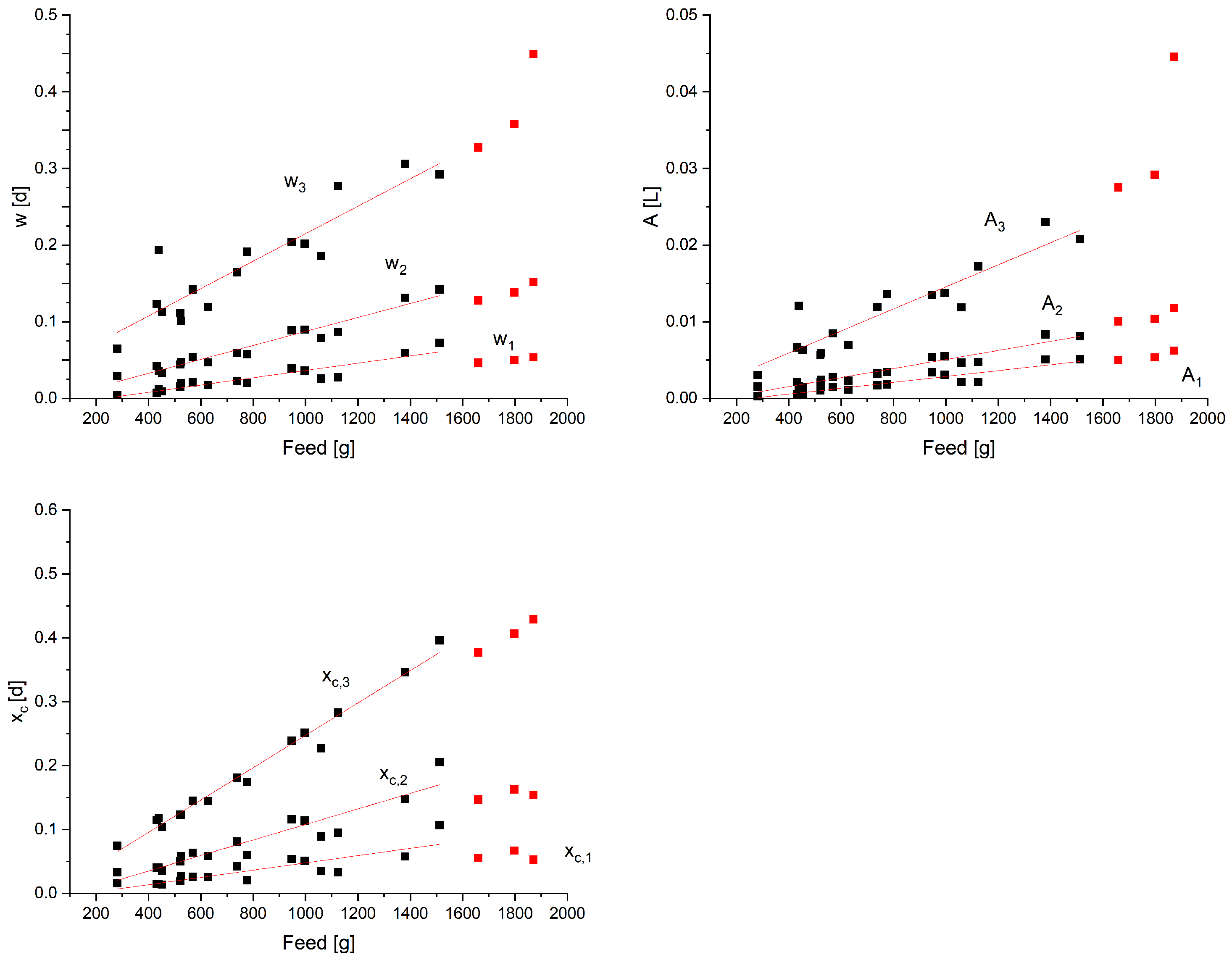
2.4. Deconvolution of Gas Production Rates and Correlation Analysis

A 1:1 mixture of primary sludge and excess sludge was fed into the reactor daily over a period of 21 days. The biogas quantities were automatically recorded in an interval of 5 min. All values of the gas production rate > $3.0$ NL/$\mathrm{h}$, which occurred because of the gas displacement by the feed were deleted from the raw data. Origin 2019 was used for mathematical deconvolution. Deconvolution is a transformation process in which a function is split into several sub-functions using mathematical operators. The sum of the sub-function returns the original function vice versa. This method is used, for example, in spectroscopy to separate overlapping peaks in order to quantify substances in heterogeneous samples. Gaussian fit was chosen for deconvolution. Gaussian function $G\left(x\right)$ is defined as (2):

$$G\left(x\right)=y_0+\frac{A}{w·{\left(\frac{\pi }{2}\right)}^2}{e}^{\frac{-2{(x-x_c)}^2}{w^2}}$$

(2)

y	peak baseline
w	peak width
A	peak area
$x_c$	peak center

Deconvolution was executed starting from the time where the substrate was introduced into the digester until approximately two hours after the gas production curve reached an almost steady-state. The course of gas production rate was split into three Gaussian curves The parameters $w_i,A_i,x_{c,i}$ obtained from the deconvolution were examined for a correlation to the amount of substrate added to the reactor.

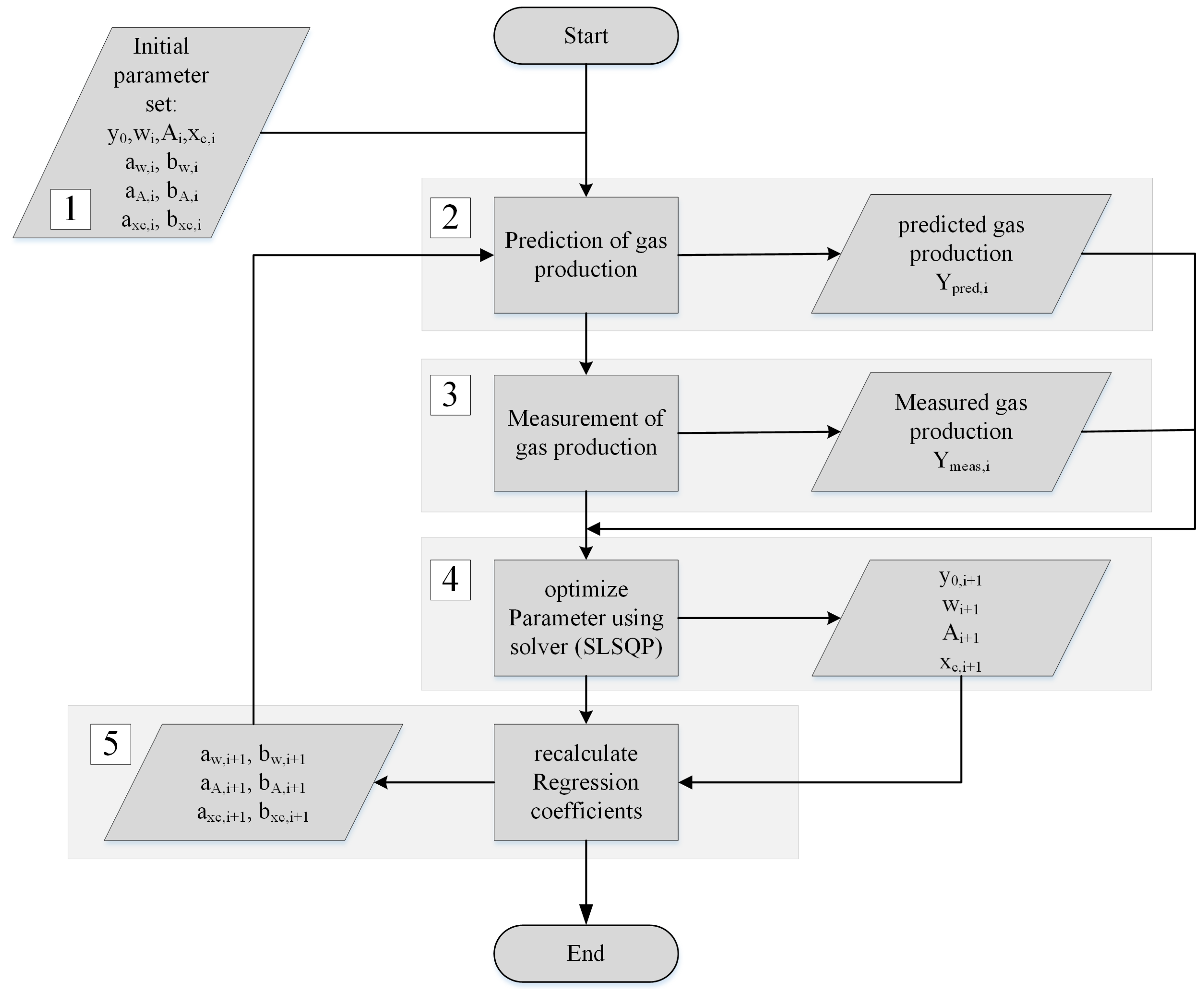
2.5. Derivation of a Model Scheme and Implementation in Python

Based on the previous investigation a model schema is proposed and was implemented in python. Parameters were optimized within Python using scipy.optimize. The optimization problem was solved using Sequential Least-Squares Programming (SLSQP) [26]. Optimization objective was to minimize the mean squared deviation between the measured gas production values and the predicted values across all data points (Equation (3)). The model was validated using the same data as described above. As initial parameters the values of the first three feeding events received from the deconvolution with Origin 2019 were taken but altered moderately.

$$obj=min\sum _{t=0}^t{(y_{measured}-y_{predicted})}^2$$

(3)

In order to avoid a possible arbitrary optimization results for example peaks becoming negative, several constraints were set. At the time of substrate feeding $t_0=0$ the following condition was set:

$$y_0+\sum G\left(t_0\right)=y_0$$

(4)

The range in which the variables can be optimized between two optimization steps was restricted. The boundaries are listed in

Table 2. Boundaries set for w${}_i$, A${}_i$ and x${}_{c,i}$.

Parameter	Boundary
$w_i$	$\pm w_{i,init}$
$A_i$	$\pm A_{i,init}$
$x_{c,i}$	$\pm \frac{x_{c,i,init}}{2}$

. Regression was calculated according to the Equations (6)–(8).

$$y=a+b·x$$

(5)

$$b=\frac{\sum x_i·y_i-n·\overline{x}·\overline{y}}{\sum {x_i}^2-n·{\overline{y}}^2}$$

(6)

$$a=\overline{y}-b·\overline{x}$$

(7)

3. Results and Discussion

3.1. Doping of Sewage Sludge with Glycerin

It was assumed that the peaks can quantitatively be assigned to certain substance groups and their underlying degradation processes and that the area of the occurring peaks is linearly dependent on the amount of substrate added. Figure 2 shows exemplarily gas production rates after directly feeding glycerin in (a) and after feeding raw sludge which was spiked with glycerin (b). Obviously, the peak in (a) which occurs around 12.5 h after the feed is related to glycerin. In (b) the first series of peaks occuring between 0 and 7.5 h is characteristic for sewage sludge as observed in several publications in the literature [24,27]. The second peak in (b) is related to glycerin once again. Although there is a clear influence of the raw sludge on the shape of the glycerin peak there is still a clear similarity given in the shape and the time-dependent occurrence in comparison to the glycerin peak in (a). Looking at the area of the intersection of both courses (a) and (b) and the glycerin course in (a), the ratio of the two areas is almost directly proportional to the amount of glycerin. This substantiates to some extent the idea that peaks can be assigned to substance groups. Furthermore, the idea and these results are so far in good agreement with today’s knowledge of biological degradation processes of different substrates and the different kinetic constants. Specific substances (e.g., proteins, lipids, carbohydrates) are following specific degradation and metabolic pathways with the involvement of specific microorganisms and enzymes. It is understandable that the different kinetics have to lead to different time frames where methane is produced from specific substrates. Yet it is known that specific substrates will have an influence on metabolic pathways. It was shown that carbohydrates will have an influence on the degradation process of proteins [28,29] which will blur specific patterns. Also there will be a change in the microbial community and thus in the specific patterns with changing substrate composition [30,31,32]. So a key factor in observing specific patterns in the course of gas production rates is the rate and extent of substrate alteration in time.

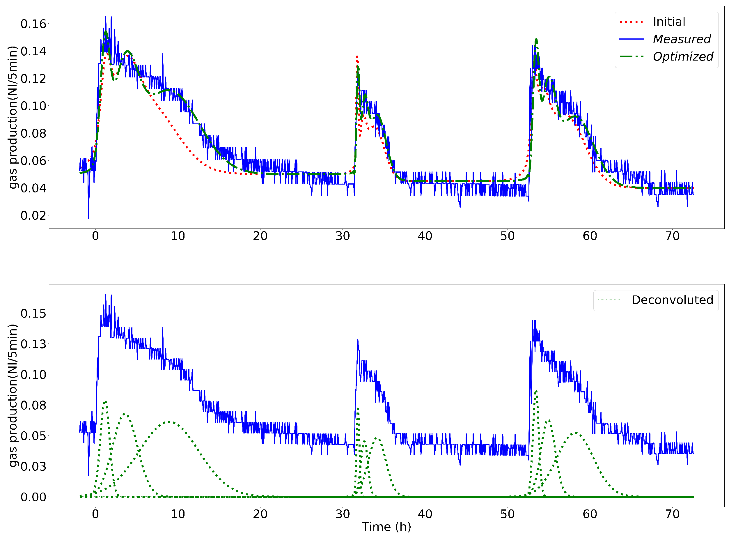
3.2. Deconvolution of the Course of Gas Production Rates and Correlation Analysis

The preliminary test described above gave rise to the idea of disassembling the course of gas production rates into individual functions and to the question of how the individual functions are related to different fractions of the substrate used.

First, the curves of the gas production rate, which were already available from various experiments in the past, were evaluated. The different curves were fitted with different functions, including the Lorentz, Voigt, LogNormal and Gaussian functions. Although all functions partially showed good fitting properties as well, they didn’t seem to be as robust using Origin 2019 as the Gaussian fit and failed to properly fit the course of production rate in many cases. However, these functions could still be taken into account in further studies. According to the OL differences in the distinctness of the curves can be observed. This showed that the density of the data points is of great importance for characterizing the curves. With high OLR, a data density of 15-min intervals is sufficient. If the organic load per feed is reduced to less than 1 kgTVS/(m${}^3$$·$d), a higher resolution of 5-min intervals and less is required. Furthermore, it turned out that a fit with two Gaussian functions provided sufficiently good results for low OLR < 1.0 kgTVS/(m ${}^3$$·$d). However, three Gaussian functions were required for higher organic loads. Throughout the recommended values for the OLR according to DWA M 368 [25] curves could be described by three Gaussian functions as shown in Figure 3.

To estimate the correlation between the parameters of the Gaussian functions and the amount of feed, varying amounts of raw sludge were added daily to the reactor and each resulting curve was broken down into three functions using Gaussian fit as described above. In total, 19 days respectively 20 feeding events were evaluated. The raw data of the gas production rates within 20 days is shown in Figure 4. The extreme values observed in the plot can be explained by the gas measurement system analyzing gas composition every 6 h and displaced volume by the feed. Only extreme values above $3.0$ NL/h were eliminated from the data set (see Figure 4). HRT and the resulting OLR were moderate being 15 days and 3.2 kgTVS/(m${}^3$$·$d) averaged over the observation time. These values are within the recommended range as described in the literature. Nevertheless, for individual feeding events recommended values were clearly exceeded. The reactor was in a stable state throughout the experiment showing a low concentration of organic acids of less than 100 mg/L and normal concentrations of methane of 65% on average in the gas phase. Specific gas production was 420 NL/kgTVS which is an average value for an anaerobic digester. Gas production curves were well pronounced. Depending on the amount of substrate added, the curves were observable between 4 h (Peak 4) at an organic load of 0.86 g TVS/L per feed and 25 h at an organic load of 6.5 g TVS/L per feed (Peak 15). The maximum gas production rate was between 1.2 NL/h and 2.04 NL/h occurring after 25 and 70 min after feeding. The baseline of the gas production rate was between 0.46 and 0.66 NL/h. Depending on the amount of substrate added, the total area of the curve contributed between 36% and 68% to the total gas volume within the time when the curve was observable. The COD equivalents of the peak area ranged between 3 g COD and 33 g COD calculated with a specific methane production of 0.35 m${}^3$ CH ${}_4$/kgCOD${}_{degraded}$ [2]. The amount of COD of the added substrate ranged from 13 g COD to 100 g COD per feed. On average, the COD-equivalent of the curves, which corresponds to degraded COD, was around 25% (20–37%) of the COD of the substrate added. After the curve the gas production rate turns into a linear slope. Figure 4 shows an example of the COD balance for the gas production rate curve 7.

From 20 analyzed gas production rate curves 19 curves could successfully be deconvoluted. The only curve that couldn’t be deconvoluted was at an OLR of $6.7$ g TVS/L (Peak 15) due to the high OLR as well as the circumstance that the rate didn’t return to the level of the baseline prior to the next feeding event. As expected, the peak area A and the width w increased with the amount of substrate added. Furthermore, a slight right shift on the time axes was observed for $x_c$ the higher the feed. The correspondingly derived parameters $w_i,A_i,x_{c,i}$ were plotted against the amount of substrate added. The result is shown in Figure 5. A linear dependency is observed for all parameters.

Nevertheless, from an OLR of 5 g TVS/L on, the linearity is increasingly lost for several parameters e.g., $w_1$, $x_{c,2}$ (see Figure 5). It is assumed, that linearity would have been given for all parameters if the feeding interval would have been increased between feeding events 15 and 16. Because these values were far outside the recommended range, they were not included in the calculation of R². In future works, it could be assessed to what extent these findings could be used in order to identify digester overloading. Furthermore, curve 16 was supposed to be influenced by the feeding event 15 which could be an explanation that 16 also differed to a greater extent from the regression line. R² ranged between 0.73 and 0.98 indicating linearity verifying the assumptions made. An overview of all R² is given in

Table 3. Determined $R^2$-values for $w_i,A_i,x_{c,i}$ in relation to the amount of substrate added.

Peak	${\mathit{w}}_{\mathit{i}}$	${\mathit{A}}_{\mathit{i}}$	${\mathit{x}}_{\mathit{c}}{,}_{\mathit{i}}$
1	0.86	0.95	0.83
2	0.87	0.93	0.84
3	0.73	0.80	0.98

. During the experiment, the reactor was in a steady state, which means it was already adapted to the substrate. It is intuitive that in this case, the total peak area A which is representing the gas production especially of easily degradable fractions should be in a linear relationship with the amount of substrate added if substrate composition doesn’t change. For the given equilibria, stoichiometry according to Buswell [1] should apply. As the ratio between different fractions of the substrate or more precisely substances with equal degradation velocity doesn’t change, linearity should also be given for the “sub” areas $A_i$. According to first-order kinetics, the occurrence of the maximum rates on the time-axes shouldn’t change with changing input amounts. However, since the maximum gas production rates did change according to these investigations, this could mean, that the hydrolysis constants should be dependent on the amount of substrate added in first-order kinetic models. Trying to translate these findings to the processes in anaerobic digestion, a shift of the maximum production rate on the time-axes could be due to a longer mixing time at higher volumes. Since the energy provided for mixing the reactor did not vary, a corresponding dispersion of the substrate will take more time with larger amounts of substrate. Another aspect that could lead to a shift is, that different species are involved in the degradation of specific substrates. According to Fuhrer [33], who identified and quantified glucose metabolism in different bacterial species in aerobic systems, uptake velocities can differ significantly from species to species. When the supply of nutrients is low, the occurrence of the maximum turnover rates will mainly depend on those organisms that convert the quickest, while slower organisms could become more visible in the patterns of gas production rates when there is a high availability of nutrients. This could lead to a shift in the point in time of the maximum gas production rates. It could also be concluded that the different degradation pathways of a substrate, for example the degradation of glucose to acetic acid, propionic acid, butyrate, etc. (cf. [16]), are in terms of conversion rates not directly proportional to each other, depending to the amount of substrate. Production of necessary enzymes could also have an influence on $x_{c,i}$ as well as on w${}_i$. As $x_{c,i}$ is determined by the Gauss function and A has a linear character also w is supposed to have a certain linearity as those three are the only unknowns in the Gauss function. Uptake capacities could have an influence on the width w as well as the mixing. Nevertheless, the approach involves solely mathematical operations to find the best-fitting A, w and $x_{c,i}$ to characterize the gas production rate curves. This does not necessarily implement a description of the real processes in the digester. The extent to which the presented results allow statements about the possibility of deriving a quantitative assignment of the peaks to defined substrate fractions, describing the quality of the mixing or recognizing overloading and inhibitions is to be investigated in the future.

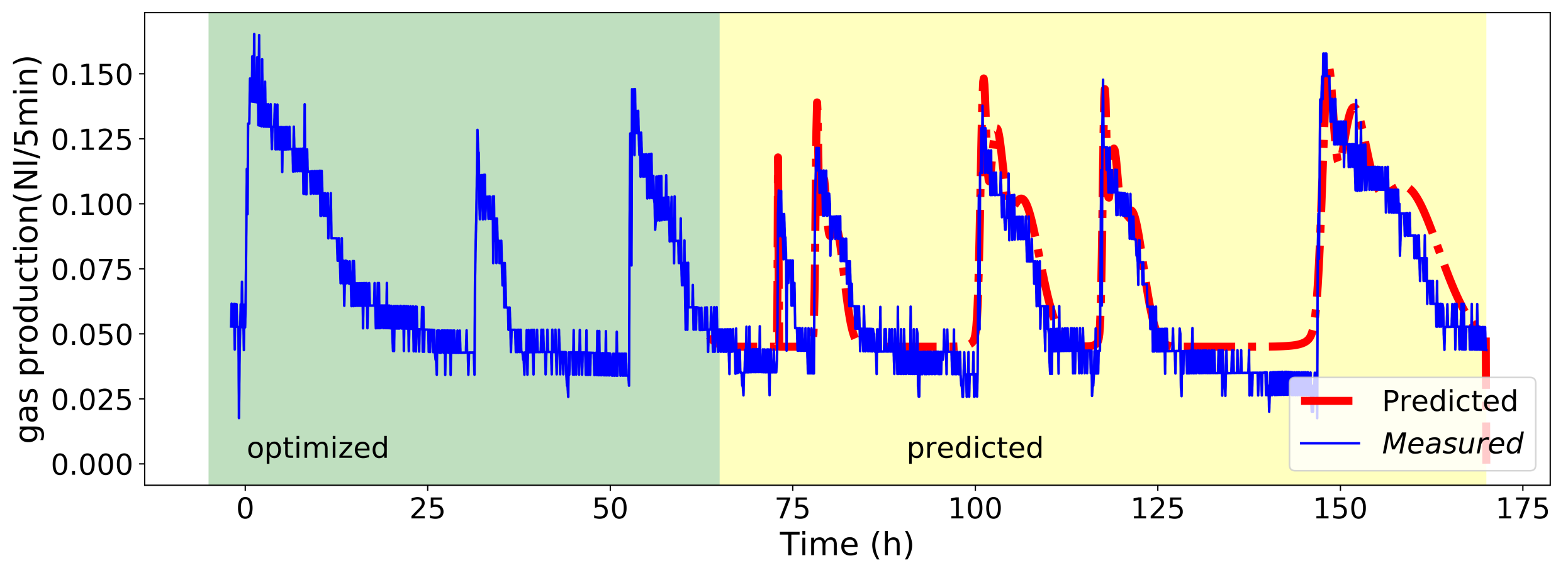
3.3. Model Scheme and Implementation in Python

The results allowed for a suggestion of a concept to predict gas production rates based on fitting previous gas production rate curves. The concept is based on the continuous sequence of five process steps:

1.

Define initial values

2.

Forecast of gas production rates with initial values

3.

Measurement of actual gas production

4.

Update values using least square fit

5.

Recalculate the regression gradient

Due to the low slope in the gas production rate following the pronounced peak, $y_0$ was defined as a constant that changes from feeding event to feeding event. The sequence is supposed to run after each feeding event. The schematic of the concept is shown in Figure 6. First, input values must be estimated (1). A forecast of the rates is calculated using the input values (2). Based on the scheduled amount of substrate $m_{input}$, the parameters of the Gauss function are calculated using the regression coefficients according to Equations (8)–(10). The gas production rate at time x can be determined according to Equation (11) by the sum of the individual Gaussian functions. The predicted rates are compared with the measured values (3) and the initially estimated parameters are optimized by minimizing the sum of squared errors for a defined time horizon (4). The coefficients of the linear regression for the Gaussian parameters are calculated based on the optimized values received from past gas production curves (5). With these values, a further forecast of the rates can be made depending on the amount of substrate added. The model could be further optimized by introducing a fourth Gaussian function representing the slow degradable fractions, replacing the baseline $y_0$. However, the solver used in this study failed to find suitable solutions for the parameters of a fourth Gaussian function, which could be due to the boundaries set or the solver itself. In order to predict the gas production of different substrates, e.g., raw sludge and a co-substrate, each substrate must go through the protocol separately. Finally, the sum of the Gaussian function is added.

$$w_i=a_{w,i}+b_{w,i}·m_{input}$$

(8)

$$A_i=a_{A,i}+b_{A,i}·m_{input}$$

(9)

$$x_{c,i}=a_{xc,i}+b_{xc,i}·m_{input}$$

(10)

$$y\left(x\right)=y_0+G_1\left(x\right)+G_2\left(x\right)+G_3\left(x\right)$$

(11)

The concept was then transferred into a Python script. A question that was still unclear was how many curves or which time horizon should be taken into account in order to optimize the values of $A,w,x_c$. The amount of feeding events respectively the time horizon is supposed to be dependent on the organic load and thus on how well the patterns are defined. Substrate characteristics will also have a major impact on the time horizon. An overall statement on the required time horizon is thus not feasible and will differ from case to case. In the following in each iteration step, three feeding events respectively three days were optimized. Figure 7 shows the result of the optimization of $w_i,A_i,x_{c,i}$ for each of the sub-functions.

For each curve, new values are obtained that can potentially be used to recalculate the regression constants as intended in step 4. It is not useful to consider all data points collected in the past, which means that in each loop several data points should be deleted and new ones should be added. In this study, regression was calculated using the parameters of the past three feeding events. The variation coefficients for regression parameters b for $w_i,A_i,x_{c,i}$ are given in

Table 4. Coefficient of variance of regression parameter b for $w_i,A_i$ and $x_{c,i}$.

Parameter	b
	%
$w_1$	51.7
$w_2$	24.7
$w_3$	31.7
$A_1$	28.9
$A_2$	18.0
$A_3$	24.0
$x_{c,1}$	28.4
$x_{c,2}$	14.6
$x_{c,3}$	10.4

. How many data points should be taken into account in order to calculate robustly the regression has still to be specified. It depends on how fast and intense substrate characteristics are changing over time on one side, and on the other on the changing dynamics of the processes within the reactor. With the regression constants, the gas production rate can now be predicted based on the amount of substrate added. Figure 8 shows the prediction and measured values in a 5-day forecast. Averaged over 6 iteration steps (with one iteration step including optimizing $w_i,A_i,x_{c,i}$ and $y_0$ for the past three gas production curves, recalculating the regression coefficients and forecasting gas production rates for the next 5 feeding events based on the scheduled amount of substrate) the difference between forecast and measured values over the period of 5 days was 5%. The coefficient of determination was calculated to be 82.9% on average over 6 iterations. This value is in a similarly good range as the results of the model presented by Lafratta [3], which were in the range of 72 and 87% within 24 h or the results by Poggio [34] using the ADM1 simulating gas production from food and green wastes (74.0–93.3%). The deep learning models introduced by Jeong et al. [11] achieved a coefficient of determination of 38 to 76%. Nevertheless, these models were used on full-scale WRRFs. The mean absolute percentage error (MAPE) averaged 17% for 6 iterations. Dittmer achieved scores of 13.87 and 18.13% with a model based on time series analysis. It must be pointed out that the scope of the investigation in this study was very limited and further data sets must be used for validation of the method described. The good prediction is also due to the fact that approx. 50% of the gas production can already be described by the baseline. It is assumed that this accuracy is sufficient to establish a feeding-management system in order to maximize the utilization efficiency of gas storage capacities. Considering that no analysis is required, the method can thus be considered very promising. However, the method cannot be used ubiquitously. While the properties of the sewage sludge will not change significantly over the course of the day, co-substrates can behave very differently. The properties can vary significantly from batch to batch. This would require substrate storage facilities of a corresponding size, so a certain degree of homogenization of the substrate properties can occur. In the case of effective feeding management a substrate storage for co-substrates is necessary after all.

As seen in the figure, predicted and measured values match very well at the beginning. The further the forecast extends into the future, the greater the deviations are becoming as the baseline changes according to the feeding history. From day 5, larger deviations between forecast and measurement are visible. This shows the need for constant recalculation in tight intervals. Table 4 shows the coefficient of variance of the parameters $w_i,A_i$ and $x_{c,i}$ calculated for 5 iteration steps. The values are high between 10 and up to 52% which is due to the small number considered for the calculation of the regression. The first Gaussian peak shows the highest variation. The first Gaussian peak is supposed to be tightly related to short-chain fatty acid (SCFA) concentration. Since it was not possible to guarantee the same acidification of the feeding samples (differences arose due to the differences in the sample quantity and the standing time before adding to the reactors), the large fluctuations can be partially explained. Nevertheless, the substrate used was homogenous over the observation period. In large-scale facilities, substrate characteristics will permanently vary to some extent leading to a higher discrepancy between forecast and measured values.

4. Conclusions

The prediction of the gas production rate in an anaerobic digester is of particular importance in order to establish a feeding management system. Due to the high analytical effort, developed models have not been able to establish themselves yet. Instead of descriptive models, simple, robust and, above all, practicable models are needed to predict gas production on large-scale facilities. As part of this work, it was shown that a good fit of the gas production rate curves is possible using the Gaussian function. The respective parameters of the Gaussian function also showed a high correlation with the amount of substrate given into the digester, which allows a prediction of the gas production rates via linear regression. The prediction can be carried out without any biological and chemical analysis. The optimization of the respective parameters is carried out continuously and thus adapts to the changing conditions of the substrate and the reactor. This system takes into account any influencing factors on gas production, without validating them since the continuous calibration is based solely on past gas volume measurements. The amount of gas displaced by the substrate added is taken into account, as is the quality of the mixing or stripping effects through continuous circulation. The method performed well. Substituting $y_0$ by a fourth Gaussian sub-function could probably further improve the performance. However, it must be noted that the investigations were carried out on experimental reactors and transferability to large-scale systems is still pending.

In this context, data-logging was not a limiting factor. Patterns were clearly observable collecting data in 5-min intervals. In large-scale facilities kinetics seems to be faster, so that the required resolution of corresponding patterns must be validated. Furthermore, large-scale facilities are much more complex and numerous influencing factors such as changes in pressure conditions, partial energy inputs from intermittent agitators can produce specific patterns themselves which could overlay patterns triggered by the feed. However, these influencing factors should be manageable and should be balanced out over a period of a few hours, which is the resolution that is relevant for an effective feeding management. Furthermore, moderate organic loads were considered within the scope of this work and robustness at higher OLR has still to be evaluated. In addition, the method was only validated on raw sludge. Transferability on co-substrates also needs further investigation. A greater challenge is the very inconsistent feeding of the digester on large scale facilities. The addition of numerous different substrates often does not follow any stringent rules and interference in the gas production patterns is supposed to occurre which could complicate finding a solution during the optimization process. In addition, unlike the experimental reactors, the feeding processes take significantly longer time, so that it could be difficult to assign the patterns to the respective event. Finally, it should be emphasized that this type of evaluation of the gas curves represents a new way of drawing conclusions about the substrate composition and the current conditions in the reactor itself. The description of existing patterns provides a very good basis for applying new mathematical/statistical approaches as well as AI especially if it is considered that continuously gas flow measurements are widely established and thus provide a huge resource of data. With this background, the assignability of different substrates to the deconvoluted peaks will be examined as well as the influence of operational parameters on $w_i,A_i$ and $x_{c,i}$.

References

1. Buswell, A.M.; Hatfield, W.D. Anaerobic Fermentation; Government Document, BULLETIN NO. 32; Illinois State Water Survey: Urbana, IL, USA, 1936. [Google Scholar]
2. Tchobanoglous, G.; Burton, F.L.; Boston, H.D.S. Wastewater Engineering: Treatment and Reuse, 4th ed.; Metcalf & Eddy Inc., Ed.; McGraw-Hill: New York, NY, USA, 2003. [Google Scholar]
3. Lafratta, M.; Thorpe, R.B.; Ouki, S.K.; Shana, A.; Germain, E.; Willcocks, M.; Lee, J. Development and validation of a dynamic first order kinetics model of a periodically operated well-mixed vessel for anaerobic digestion. Chem. Eng. J. 2021, 426, 131732. [Google Scholar] [CrossRef]
4. Gavala, H.N.; Angelidaki, I.; Ahring, B.K. Kinetics and Modeling of Anaerobic Digestion Process. In Biomethanation; Ahring, B.K., Angelidaki, I., de Macario, E.C., Gavala, H.N., Hofman-Bang, J., Macario, A.J.L., Elferink, S.J.W.H.O., Raskin, L., Stams, A.J.M., Westermann, P., et al., Eds.; Springer: Berlin/Heidelberg, Germany, 2003; pp. 57–93. [Google Scholar] [CrossRef]
5. Batstone, D.; Keller, J.; Angelidaki, I.; Kalyuzhnyi, S.; Pavlostathis, S.; Rozzi, A.; Sanders, W.; Siegrist, H.; Vavilin, V. The IWA Anaerobic Digestion Model No 1 (ADM1). Water Sci. Technol. 2002, 45, 65–73. [Google Scholar] [CrossRef] [PubMed]
6. Raeyatdoost, N.; Eccleston, R.; Wolf, C. Flexible Methane Production Using a Proportional Integral Controller with Simulation-Based Soft Sensor. Chem. Eng. Technol. 2019, 43, 75–83. [Google Scholar] [CrossRef]
7. Mauky, E.; Weinrich, S.; Jacobi, H.F.; Naegele, H.J.; Liebetrau, J.; Nelles, M. Model Predictive Control for Demand-Driven Biogas Production in Full Scale. Chem. Eng. Technol. 2016, 39, 652–664. [Google Scholar] [CrossRef]
8. Weinrich, S.; Nelles, M. Systematic simplification of the Anaerobic Digestion Model No. 1 (ADM1) – Model development and stoichiometric analysis. Bioresour. Technol. 2021, 333, 125124. [Google Scholar] [CrossRef]
9. Siegrist, H.; Vogt, D.; Garcia-Heras, J.L.; Gujer, W. Mathematical Model for Meso- and Thermophilic Anaerobic Sewage Sludge Digestion. Environ. Sci. Technol. 2002, 36, 1113–1123. [Google Scholar] [CrossRef]
10. Solomatine, D.; See, L.; Abrahart, R. Approaches and Experiences. In Practical Hydroinformatics: Computational Intelligence and Technological Developments in Water Applications; Abrahart, R.J., See, L.M., Solomatine, D.P., Eds.; Springer: Berlin/Heidelberg, Germany, 2008; pp. 17–30. [Google Scholar] [CrossRef]
11. Jeong, K.; Abbas, A.; Shin, J.; Son, M.; Kim, Y.M.; Cho, K.H. Prediction of biogas production in anaerobic co-digestion of organic wastes using deep learning models. Water Res. 2021, 205, 117697. [Google Scholar] [CrossRef]
12. Beltramo, T.; Klocke, M.; Hitzmann, B. Prediction of the biogas production using GA and ACO input features selection method for ANN model. Inf. Process. Agric. 2019, 6, 349–356. [Google Scholar] [CrossRef]
13. Güçlü, D.; Yılmaz, N.; Ozkan-Yucel, U.G. Application of neural network prediction model to full-scale anaerobic sludge digestion. J. Chem. Technol. Biotechnol. 2011, 86, 691–698. [Google Scholar] [CrossRef]
14. Andrade Cruz, I.; Chuenchart, W.; Long, F.; Surendra, K.; Renata Santos Andrade, L.; Bilal, M.; Liu, H.; Tavares Figueiredo, R.; Khanal, S.K.; Fernando Romanholo Ferreira, L. Application of machine learning in anaerobic digestion: Perspectives and challenges. Bioresour. Technol. 2022, 345, 126433. [Google Scholar] [CrossRef]
15. Dittmer, C.; Krümpel, J.; Lemmer, A. Modeling and Simulation of Biogas Production in Full Scale with Time Series Analysis. Microorganisms 2021, 9, 324. [Google Scholar] [CrossRef]
16. Gallert, C.; Winter, J. Bacterial Metabolism in Wastewater Treatment Systems. In Environmental Biotechnology: Concepts and Applications; WILEY-VCH Verlag GmbH & Co. KGaA.: Weinheim, Germany, 2004. [Google Scholar] [CrossRef]
17. Guo, H.; Oosterkamp, M.J.; Tonin, F.; Hendriks, A.; Nair, R.; van Lier, J.B.; de Kreuk, M. Reconsidering hydrolysis kinetics for anaerobic digestion of waste activated sludge applying cascade reactors with ultra-short residence times. Water Res. 2021, 202, 117398. [Google Scholar] [CrossRef]
18. Koch, K.; Drewes, J.E. Alternative approach to estimate the hydrolysis rate constant of particulate material from batch data. Appl. Energy 2014, 120, 11–15. [Google Scholar] [CrossRef]
19. Christ, O.; Wilderer, P.; Angerhöfer, R.; Faulstich, M. Mathematical modeling of the hydrolysis of anaerobic processes. Water Sci. Technol. 2000, 41, 61–65. [Google Scholar] [CrossRef]
20. Gujer, W.; Zehnder, A.J.B. Conversion Processes in Anaerobic Digestion. Water Sci. Technol. 1983, 15, 127–167. [Google Scholar] [CrossRef]
21. O’Rourke, J.; McCarty, P. Kinetics of Anaerobic Waste Treatment at Reduced Temperatures; Department of Civil Engineering: Technical Report; Stanford University: Stanford, CA, USA, 1968. [Google Scholar]
22. Garcia-Heras, J. Reactor Sizing, Process Kinetics and Modelling of Anaerobic Digestion of Complex Wastes. In Biomethanization of the Organic Fraction of Municipal Solid Wastes; IWA Publishing: London, UK, 2003. [Google Scholar]
23. Vavilin, V.; Fernandez, B.; Palatsi, J.; Flotats, X. Hydrolysis kinetics in anaerobic degradation of particulate organic material: An overview. Waste Manag. 2008, 28, 939–951. [Google Scholar] [CrossRef]
24. Hubert, C.; Steiniger, B.; Schaum, C. Residues from the Dairy Industry as Co-Substrate for the Flexibilization of Digester Operation. Water Environ. Res. 2019, 92, 534–540. [Google Scholar] [CrossRef]
25. Deutsche Vereinigung für Wasserwirtschaft, Abwasser und Abfall e.V. Code of practice DWA-M 368: Biological Stabilization of Sewage Sludge (“Merkblatt DWA-M 368: Biologische Stabilisierung von Klärschlamm”); Deutsche Vereinigung für Wasserwirtschaft, Abwasser und Abfall e. V.: Hennef, Germany, 2014; ISBN 978-3-944328-60-7. [Google Scholar]
26. Virtanen, P.; Gommers, R.; Oliphant, T.E.; Haberland, M.; Reddy, T.; Cournapeau, D.; Burovski, E.; Peterson, P.; Weckesser, W.; Bright, J.; et al. SciPy 1.0: Fundamental Algorithms for Scientific Computing in Python. Nat. Methods 2020, 17, 261–272. [Google Scholar] [CrossRef]
27. Lafratta, M.; Thorpe, R.B.; Ouki, S.K.; Shana, A.; Germain, E.; Willcocks, M.; Lee, J. Dynamic biogas production from anaerobic digestion of sewage sludge for on-demand electricity generation. Bioresour. Technol. 2020, 310, 123415. [Google Scholar] [CrossRef]
28. Deng, Z.; Poulsen, J.S.; Nielsen, J.L.; Spanjers, H.; van Lier, J.B. Unveiling AD mysteries: Why protein conversion is retarded when carbohydrates are present? In Proceedings of the International Water Association, 17th World Congress on Anaerobic Digestion, Ann Arbor, 17–22 June 2022.
29. Breure, A.M.; Mooijman, K.A.; van Andel, J.G. Protein degradation in anaerobic digestion: Influence of volatile fatty acids and carbohydrates on hydrolysis and acidogenic fermentation of gelatin. Appl. Microbiol. Biotechnol. 1986, 24, 426–431. [Google Scholar] [CrossRef]
30. Dargode, P.S.; More, P.P.; Gore, S.S.; Asodekar, B.R.; Sharma, M.B.; Lali, A.M. Microbial consortia adaptation to substrate changes in anaerobic digestion. Prep. Biochem. Biotechnol. 2022, 52, 924–936. [Google Scholar] [CrossRef] [PubMed]
31. De Francisci, D.; Kougias, P.G.; Treu, L.; Campanaro, S.; Angelidaki, I. Microbial diversity and dynamicity of biogas reactors due to radical changes of feedstock composition. Bioresource Technology 2015, 176, 56–64. [Google Scholar] [CrossRef] [PubMed]
32. Li, L.; He, Q.; Ma, Y.; Wang, X.; Peng, X. Dynamics of microbial community in a mesophilic anaerobic digester treating food waste: Relationship between community structure and process stability. Bioresour. Technol. 2015, 189, 113–120. [Google Scholar] [CrossRef] [PubMed]
33. Fuhrer, T.; Fischer, E.; Sauer, U. Experimental identification and quantification of glucose metabolism in seven bacterial species. J. Bacteriol. 2005, 187, 1581–1590. [Google Scholar] [CrossRef]
34. Poggio, D.; Walker, M.; Nimmo, W.; Ma, L.; Pourkashanian, M. Modelling the anaerobic digestion of solid organic waste— Substrate characterisation method for ADM1 using a combined biochemical and kinetic parameter estimation approach. Waste Manag. 2016, 53, 40–54. [Google Scholar] [CrossRef]
Figure 1. k h y d -values for carbohydrates, proteins and lipids evaluated by Christ et al. [19] (a), Gujer [20] with data of O’Rourke [21] (b) and Garcia-Heras [22] in [23] (c).
Water 15 00614 g001
Figure 2. Course of the gas production rate after feeding the reactor with glycerin (a) and after feeding with a sewage sludge sample spiked with glycerin (b). The diagram below shows the intersection of (a) and (b).
Water 15 00614 g002
Figure 3. Deconvolution of gas production rate curve 7 into three gaussian functions; COD-balance: Percentages represent the share of the COD-equivalents of the deconvoluted peaks on the amount of COD of the feed. For better illustration the course of gas production rate was flattend.
Water 15 00614 g003
Figure 4. Gas production rates during 20 days of reactor operation. Blue dots are representing the extreme values due to the feeding. The numbers are a sequential numbering of the gas production rate curves that occur after feeding. For better visualisation feeding events 8 to 12 were excluded.
Water 15 00614 g004
Figure 5. Linear relationship between w i , A i , x c , i and the amount of substrate added. Red dots represent OLR > 5 kg TVS/L. They were not taken into account in calculating R 2 .
Water 15 00614 g005
Figure 6. Proposed model scheme for prediction of gas production rates consisting of 5 steps.
Water 15 00614 g006
Figure 7. Gaussian fit of the curves 1, 2 and 3 (see Figure 4). Upper figure shows the fitted gas production rate course (green) in comparison to the measured (blue) and the course calculated with initial values (red). Lower figure shows the separated Gaussian functions (green) for each curve.
Water 15 00614 g007
Figure 8. Prediction of gas production rates from 5 feeding events. The first three curves are used to optimize the Gaussian parameters (green). Based on the optimized values the following 5 curves are predicted (yellow).
Water 15 00614 g008