
An Interpretable Recurrent Neural Network for Waterflooding Reservoir Flow Disequilibrium Analysis
by
 , and
, and
Yunqi Jiang
1,
Wenjuan Shen
2,
Huaqing Zhang
3,
Kai Zhang
1,4,*,
Jian Wang
3,* and
Liming Zhang
1 1
School of Petroleum Engineering, China University of Petroleum East China—Qingdao Campus, Qingdao 266580, China
2
Dagang Oilfield Group Ltd. Company, Tianjin 300280, China
3
College of Sciences, China University of Petroleum East China—Qingdao Campus, Qingdao 266580, China
4
School of Civil Engineering, Qingdao University of Technology, Qingdao 266520, China
*
Authors to whom correspondence should be addressed.
Water 2023, 15(4), 623; https://doi.org/10.3390/w15040623
Submission received: 14 January 2023
/
Revised: 1 February 2023
/
Accepted: 2 February 2023
/
Published: 5 February 2023
(This article belongs to the Section Urban Water Management)
Abstract
:Waterflooding is one of the most common reservoir development programs, driving the oil in porous media to the production wells by injecting high-pressure water into the reservoir. In the process of oil development, identifying the underground flow distribution, so as to take measures such as water plugging and profile control for high permeability layers to prevent water channeling, is of great importance for oilfield management. However, influenced by the heterogeneous geophysical properties of porous media, there is strong uncertainty in the underground flow distribution. In this paper, we propose an interpretable recurrent neural network (IRNN) based on the material balance equation, to characterize the flow disequilibrium and to predict the production behaviors. IRNN is constructed using two interpretable modules, where the inflow module aims to compute the total inflow rate from all injectors to each producer, and the drainage module is designed to approximate the fluid change rate among the water drainage volume. On the spatial scale, IRNN takes a self-attention mechanism to focus on the important input signals and to reduce the influence of the redundant information, so as to deal with the mutual interference between the injection–production groups efficiently. On the temporal scale, IRNN employs the recurrent neural network, taking into account the impact of historical injection signals on the current production behavior. In addition, a Gaussian kernel function with boundary constraints is embedded in IRNN to quantitatively characterize the inter-well flow disequilibrium. Through the verification of two synthetic experiments, IRNN outperforms the canonical multilayer perceptron on both the history match and the forecast of productivity, and it effectively reflects the subsurface flow disequilibrium between the injectors and the producers.
1. Introduction
Waterflooding is known as “secondary recovery”, aiming to inject water into the reservoir to maintain the formation pressure close to the initial pressure, and to displace oil from the rock pores. Characterizing the flow disequilibrium between injection and production wells, and identifying the high conductivity channels, is the fundamental work to take hydrodynamic adjustment measures, such as water plugging. In this way, water channeling in production wells can be effectively prevented, and the oil recovery of the reservoir can be enhanced. Therefore, it is an important work of oilfield management to invert the non-equilibrium of underground flow, by using the dynamic rate and pressure signals, which are the most easily obtained data in the oilfield. For an oil reservoir, the injection signals such as bottom hole pressure (BHP) and water injection rates (WIRs) of the injectors can be regarded as the interference to the geological system, and the BHP and liquid production rates (LPRs) of producers can be regarded as the feedback. The multiphase flow in porous media is a complex and invisible process with strong uncertainty, because the flow distribution is affected not only by the fluid properties (such as viscosity) [1,2], but also by the heterogenous petrophysical properties (such as porosity, permeability, etc.) of the formation [3,4,5].
The complex nonlinear correlation between injection and production signals is mainly reflected in two aspects: the spatial and temporal scale of the oil reservoir development. On the spatial scale, the injection–production signals constitute a complex nonlinear system, where the production behaviors are not only decided by multiple injection wells, but also influenced by the mutual interference from surrounding producers. Specifically, if an injector-producer group is in the high permeability area, the injected water can easily flow to the production well along the high conductivity channel. Hence, the dynamic signals of this injector are of great significance to the production behaviors of the producer. However, if there are no connecting relationships between some injectors and the analyzed producer, the injection signals may be useless or even detrimental to the analysis of the productivity behaviors of this producer. On the temporal scale, the injection–production signals are typical time series data, and the injected water needs a period of time to reach the bottom of the producers, so the production signals have a certain time lag. In other words, the historical water injection would influence the current production signals. The reservoir numerical simulators can accurately reflect the underground flow disequilibrium, but they are based on grid computing, requiring the permeability, porosity, saturation and other geological properties of each grid, which are very expensive to acquire through well logging. Additionally, with the increase in reservoir scale, the calculation cost of the numerical simulator also increases, and it takes tens of minutes or even hours to complete a simulation [6]. To save modeling time and economic cost, a series of models for finding injection production mapping relationships have been proposed, mainly including: reservoir-seepage-knowledge-based models and machine-learning (ML)-based models.
Developed on the material balance partial differential equations (PDEs), Yousef, Gentil, and Jensen and Lake [7] propose the capacitance resistance model (CRM), aiming to use the BHP (both injectors and producers) and WIRs data to approximate the LPRs for each producer. CRM employs the time constant and connectivity coefficient to indicate the time lag and attenuation of the LPRs to the BHP and WIRs, and the volume fraction of injected water between each injection well and a specified production well. Based on the primary CRM, a number of variants have been put forward in the last decade. Naudomsup and Lake [8] incorporate the miscible-displacement-theory-based tracer model with CRM, increasing the precision of tracer matching. In this combined model, both the small-scale heterogeneity and large-scale heterogeneity can be characterized by the Péclet number and the Koval factor, respectively. Temizel, Artun, and Yang [9] combine the Buckley–Leverett theory with CRM, deriving an oil fractional-flow function with the Y-function, improving the CRM’s performance on oil rate forecast. Gubanova, Orlov, Koroteev, and Shmidt [10] modify the original CRM by replacing the constant connectivity weights with changeable ones, which widens the applicability, such as the shut-in and workover stages. Moreover, the modified CRM adopts the vectorized form and advanced optimization technology, effectively speeding up the training procedure. Based on CRM, Arouri, Lake and Sayyafzadeh [11] propose a bilevel approach to solve the bilevel optimization of well placement and control settings. On the inner loop, Adam-simultaneous perturbation stochastic approximation (SPSA) is employed to assist CRM to optimize the injection–production schedule. On the outer loop, CRM adopts the particle swarm optimization (PSO) algorithm to generate different initial well location solutions, and to optimize these solutions until it finds the well placement scheme with biggest net present value (NPV).
The inter-well numerical simulation model (INSIM) is another important physical knowledge-based model, which simplifies the reservoir into a number of volume flow units, avoiding the complicated and time-consuming grid calculation of commercial simulators [12]. Derived from the Buckley–Leverett theory and the material balance equation, INSIM can both infer the flow disequilibrium of each injector–producer pair, and forecast the production behaviors (LPRs and water cut). To extend the performance and applicability of INSIM, INSIM with front tracking, INSIM-FT [13,14] is proposed, outperforming INSIM on saturation computation and history matching; INSIM-FT-3D [15] considers the gravity effect and can be used in the simulation of three-dimensional waterflooding reservoirs; INSIM-BHP [16] can provide accurate history matching, prediction, and injection–production optimization for a 3D waterflooding reservoir with slanted wells.
Machine-learning (ML)-based approaches are expected to model the complicated injection–production relationships via their powerful learning ability. The multilayer perceptron (MLP) is used in the simulation of waterflooding reservoirs, which can reflect the inter-well connectivity by computing the products of the weight matrices between the input-hidden-layer and hidden-output-layer [17,18]. Furthermore, Mo et al. [19] employ a deep convolutional encoder–decoder network to evaluate the uncertainty of the subsurface flow among the porous media, to tackle the high-dimensional saturation discontinuity problems in the surrogate strategies. Carpenter [20] adopts a long short-term memory (LSTM) to estimate the multiphase flow rates and back-allocation, which obtains great accuracy in both the simulated and actual field data. Based on Bayesian Markov chain Monte Carlo (MCMC) and LSTM, Zhang et al. [21] propose Bayesian-LSTM MCMC to reduce the uncertainty in subsurface flow modeling, improving the accuracy and robustness of the workflow. These machine-learning approaches could effectively model the mapping relationships from water injection signals to production signals via their powerful learning ability. Furthermore, the challenge for these machine-learning models is that seldom seepage-physics-knowledge is considered in the model’s learning framework, so that the interpretability of the modeled results cannot be guaranteed.
To combine the merits of reservoir-seepage-knowledge-based models and machine-learning models, we propose an interpretable recurrent neural network (IRNN). The proposed model adopts a novel learning framework embedded with the material balance equation, and incorporates an inflow module and a drainage module to simulate the multiphase flow behaviors. The inflow module aims to calculate the total inflow rate from every injector to the specific producer, and the drainage module is used to simulate the fluid change rate of the water drainage volume. Furthermore, the self-attention mechanism is used in IRNN to help the model to focus on the important information of the WIRs and the BHP signals, effectively considering the impact of mutual interference between injector–producer groups on the reservoir spatial scale. In addition, IRNN utilizes the recurrent neural network structures to memorize the valuable information of the historical input data, so as to improve the performance on predicting complex time series (such as water cut). Furthermore, a Gaussian kernel function is introduced in the proposed model to measure the flow disequilibrium, which takes account into the boundary constraint to ensure the rationality of the characterization results.
The rest of this paper is laid out as follows. Section 2 introduces the material balance equation and the development of IRNN. The performance of the proposed model and the traditional ML-based model (MLP) on two synthetic models, including the three-channel model and Olympus model, are demonstrated and discussed in Section 3. Finally, we summarize this paper in Section 4.
2. Methodology
2.1. Material Balance Equation of the Waterflooding Reservoir
For a waterflooding reservoir, the production behaviors of the producers are mainly affected by two aspects: the water injection effect and the fluid change effect of the drainage volume (caused by the compressibility of the porous media and fluids). Considering the waterflooding reservoir as a geological system with a closed boundary, and assuming that there are S injectors and Q producers, the productivity of producer q can be expressed as:
where s and q are the indexes of the injectors and producers, respectively; is the average formation pressure, t is the time step, C represents the total compressibility coefficient of the porous media and fluids, V is the water drainage volume, i(t) and o(t) are the water injection rates (WIRs) and liquid production rates (LPRs), respectively, and denotes the disequilibrium factor, which is the injection volume fraction from injector s toward producer q. means that the sum of the injection volume fractions for each injector equals 1. Equation (1) is the material balance equation for the waterflooding reservoir, which is the foundation of the reservoir-seepage-knowledge-based models. As mentioned above, the LPRs mainly come from the contributions of two parts: the water injection effect (the first right-hand item) and the fluid change effect of the drainage volume (the second right-hand item).
For given injectors and producers, C and V in Equation (1) can be regarded as constants, so that the fluid change effect can be seen as a function of the average formation pressure , and time t:
where represents the fluid change effect among the drainage volume, and () is the mapping function from t to . During the oil development process, the average formation pressure is influenced by the water injection of the injectors, and the liquid production from the producers. In the oil field, the most available data are the WIRs, LPRs, and bottom hole pressure (BHP). Therefore, in IRNN, we propose the use of the WIRs and BHP data of injectors and producers to approximate Equation (2):
where and are the BHP data of the injection wells and production wells, respectively, and () represents the nonlinear mapping function.
2.2. Development of the Interpretable Recurrent Neural Network
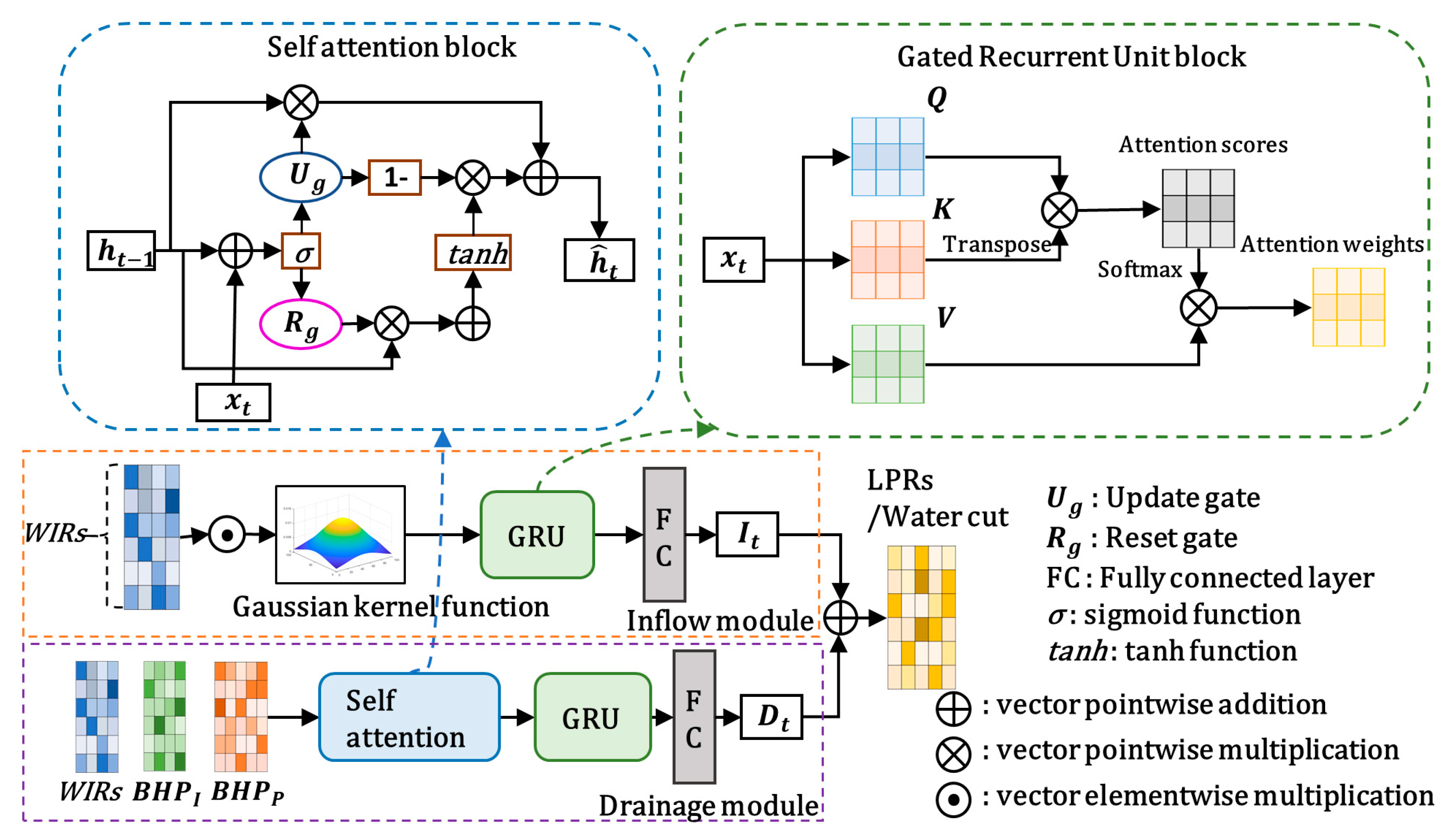
In the spatial scale of the waterflooding reservoir, the production behaviors of each producer are not only determined by its production schedules, but they are also influenced by the signals of other injectors and producers. Thus, the mutual interference of injector–producer groups should be considered in the simulation of the underground multiphase flow of the porous media. Furthermore, the injection and production signals can be recognized as the disturbance and the feedback of the underground geological system, which are complicated nonlinear time series with time lags. The injected water has to flow through the heterogeneous formation for several days, and even several weeks, to reach the bottom of the production wells. Therefore, the production signals are affected by the continuous historical injection signals on the temporal scale. The structures of IRNN are shown in Figure 1, including the inflow module and the drainage module. To take the mutual interference of injector–producer groups into account, the self-attention mechanism is introduced in IRNN to make the model pay more attention to the vital injection–production information. In addition, the recurrent neural network block is used in IRNN to enhance the ability to tackle time series data, by memorizing important historical dynamic signals. Thus, coupling the inflow module and the drainage module, IRNN can simulate the production behaviors based on the material balance equation.
The fluid change effect on the drainage volume is approximated by the drainage module, as shown in Figure 1. We use E = {} to indicate the input data set of the drainage module. The self-attention block can assign different attention weights to the input data, E, thereby making IRNN focus on the features that have important influences on the productivity signals. There are three matrices in the self-attention block, as shown in Figure 1, as denoted by Q, K, and V, which are transformed from the input vectors by the vectors of queries, keys, and values. The attention weights are computed by:
where is the number of columns of K, and T represents the transpose operation.
The gated recurrent unit (GRU) is a variant of LSTM, which has similar fitting and predicting accuracy, but uses simplified model structures. GRU adopts the update gate to decide how much information of the past data needs to be transferred to the future, and employs the reset gate to determine how much of the past data to forget. In this way, the important response signals of the past data can be preserved, and the redundant or useless signals would be eliminated. The update gate is calculated by:
where and are the weight matrices of the update gate for the current input and the previous hidden state , respectively; and is the sigmoid activation function.
The reset gate is computed as follows:
where and are the weight matrices of the reset gate for the current input and the previous hidden state .
Then, the candidate hidden state can be calculated based on Equations (5) and (6):
where and are the weight matrices of the current hidden state, and denotes the vector elementwise multiplication.
Next, the new memory content can be given as:
With the given input data set E, the drainage module can obtain the attention weights via the self-attention block, and the weights are fed to the GRU block to generate the , and then through a fully connected (FC) layer to generate the fluid change rate among the drainage volume, :
where () and represent the computation provided by the self-attention block and GRU block, respectively, is the weight matrix of the fully connected layer in the drainage module.
The inflow module aims to compute the total inflow rates to the considered producer, and to characterize the disequilibrium factors, . In this module, we adopt a Gaussian kernel function with zero mean and unit variance to quantitively evaluate the injection volume distribution ratio for each injector–producer group, which can be expressed as:
Assuming that there are S injectors and Q producers, the matrix of the disequilibrium factors, , can be written as:
The motivation for using the Gaussian kernel function to infer the disequilibrium factors comes from the study of feature selection in the machine learning field. Chakraborty and Pal [22] propose using an exponential function to select the important features, because these monotonic differentiable functions would allocate large values to the features that are important to the learning task, and assign small values to the redundant or harmful features. Similarly, the important vectors of the corresponding injectors in WIRs, are expected to obtain big values via the Gaussian kernel function. In this way, the inter-well flow disequilibrium can be characterized in the inflow module, where the bigger the disequilibrium factor, the bigger the injection volume fraction of the injector-producer group. With the given WIRs data, the final output of the inflow module can be computed through the Gaussian function, a GRU block, and a fully connected layer in turn, which can be given as:
where is the weight matrix of the fully connected layer in the inflow module.
According to the material balance equation, the modeled LPRs can be obtained from the outputs of the inflow module and the drainage module, as shown in Figure 1:
where represent the estimated LPRs for the production wells. In this paper, we take the mean square error (MSE) function as the loss evaluation function, and considering the boundary constraint of the disequilibrium factors, the total loss function of IRNN can be written as:
where T is the length of the time steps; and is the coefficient of the regularization item. It should be noted that we still use this framework to estimate and to forecast the water cut of the production wells, where the outputs are replaced by the water cut data. The training pseudocode for IRNN is demonstrated in Algorithm 1.
| Algorithm 1: The training pseudocode for IRNN. | |
| Input:WIRs, water injection rates; BHPI and BHPP, BHP data of the injectors and producers, respectively Output: Estimated liquid production rates, | |
| 1 | / Start training / |
| 2 | While stop criteria is not met |
| 3 | / Drainage module computation / |
| Calculate the fluid change rate among the drainage volume, according to Equation (9); | |
| 4 | / Inflow module computation / |
| Calculate the total inflow rates for Q producers, according to Equation (12); | |
| 5 | / Modeled liquid production rates computation / |
| Calculate the modeled liquid production rates, , according to Equation (13); | |
| 6 | / Loss evaluation / |
| Compute the total loss of IRNN, , using Equation (14); | |
| 7 | / Model parameters optimization / |
| Optimize weight matrices and the independent variables of Equation (10). | |
| 8 | End while |
| 9 | / End training / |
3. Results and Discussion
In this paper, two reservoir models are implemented to test the performance of IRNN and the classical recurrent neural network, MLP. The first model names a three-channel model, which is a two-dimensional synthetic reservoir model used in the works of [23,24]. The second model is the Olympus reservoir, which is an offshore oil field model with 16 layers in the North Sea. Both models are simulated by ECLIPSE (Schlumberger Ltd., Houston, TX, USA) in this paper. Both IRNN and MLP are implemented on a Pytorch framework by Python 3.7.6, and they are optimized using the Adam optimization algorithm. MLP takes the tanh function as the activation function, and the number of hidden layer nodes is 15. IRNN adopts the mini-batch processing method with the batch size of 10, and the detailed hyperparameters used in IRNN are listed in Table 1, which are optimized by the Hyperopt library. The candidate sets of hidden nodes of the GRU block, and hidden nodes of queries, keys, and values of the self-attention block and hidden nodes of the fully connected layer are {10, 15, 20, 25, 30}. The candidates of batch size are {5, 10, 15, 20}. The candidate sets of the initial learning rate and the coefficient of the regularization item are {0.01, 0.02, 0.03, 0.04, 0.05}. To ensure the fairness of the comparison experiments, the results shown in this paper are the average of 10 runs.
3.1. Three-Channel Model
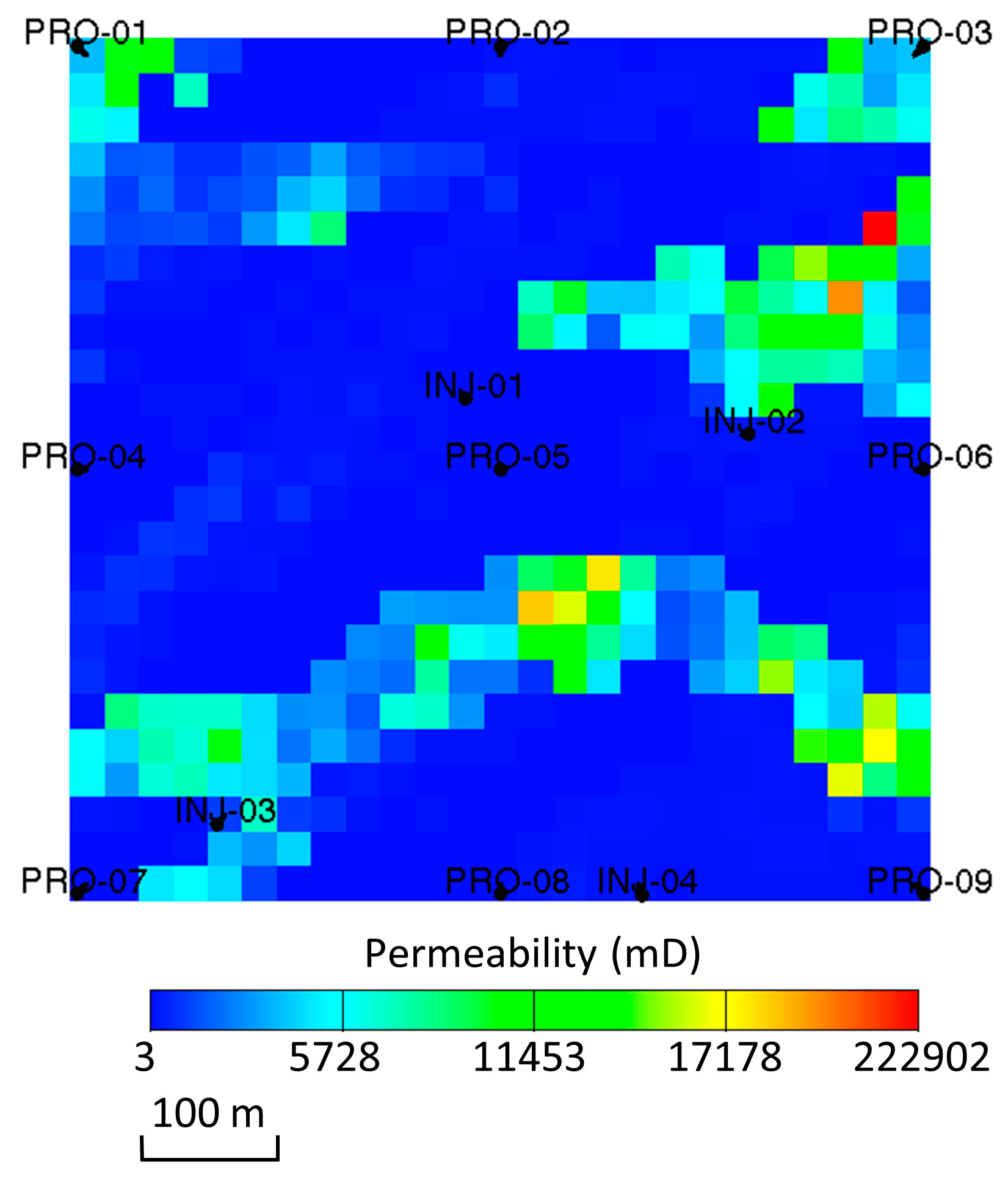
The three-channel model consists of 25 × 25 × 1 grids, with 100, 100, and 10 ft in the X, Y, and Z directions, respectively. There are four injection wells and nine production wells in this model, producing around 2670 days (1380 time steps). The porosity is 0.2 and the initial oil saturation is 0.8 for all grids, and the detailed geological properties of this synthetic model can be found in Table 2. The permeability distribution is demonstrated in Figure 2.
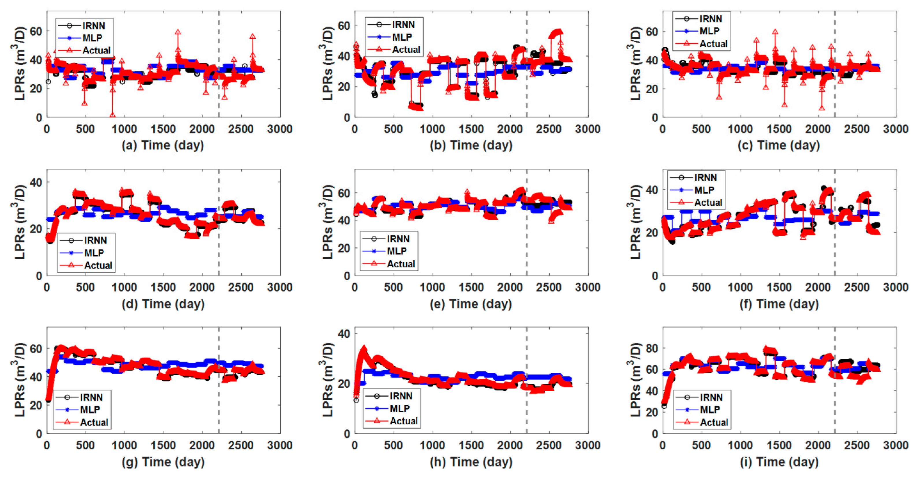
The history matching and predicting results obtained by IRNN and MLP are shown in Figure 3, which are divided by the grey dashed lines. In general, IRNN outperforms MLP on both history matching and the forecast of the liquid production rates on nine producers, since the black curves obtained via IRNN have a better consistency with the actual values (the red lines) than the blue lines obtained via MLP. In detail, MLP seems to have fair performances on the producers with relatively smooth producing rates, as shown in Figure 3a,c,e, where the general trends of the actual LPRs can be fitted and predicted via MLP. In contrast, it is difficult for this classical ML model to make a precise estimation and prediction on the other production wells with violent shocks, as shown in Figure 3b,d,f–i. These fluctuations of the LPRs signals come from the interference of the pulsed water injections, which would increase the complexity of the injection–production relationships. As shown in Figure 3, the proposed model enables to fit and to forecast the LPRs with great accuracy, not only on the producers with smooth production curves, but also on the producers with complex wave curves. The results of the LPR curves illustrate that the fitting and generalization ability of the proposed model is fully enhanced, because the self-attention mechanism can help IRNN to focus on the important injection signals on a reservoir spatial scale.
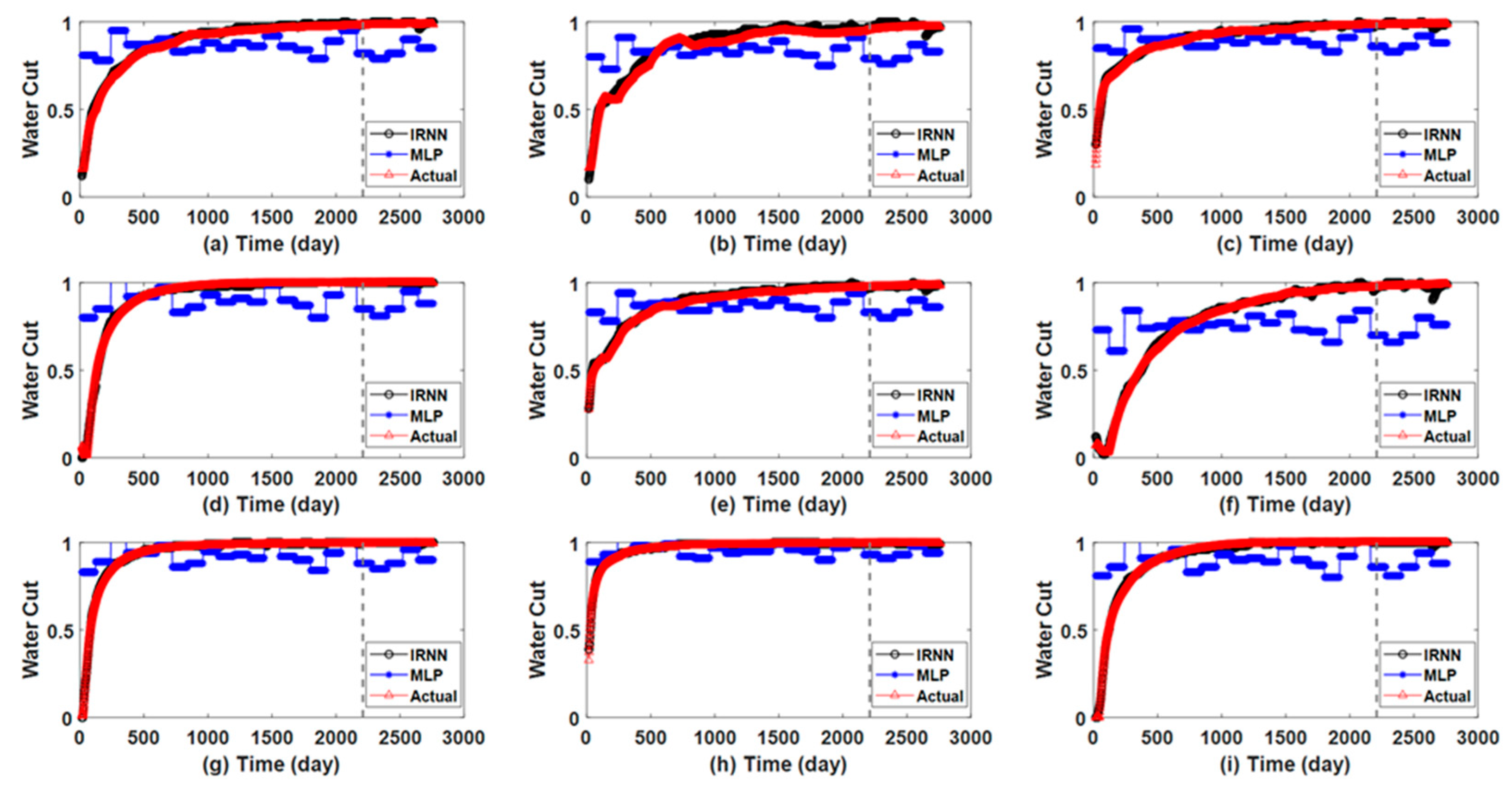
Although there is mutual interference between different injector–producer groups, the correlation between the water injection signals and the liquid production signals is still strong. This is because the total water injection volume basically equals the total liquid production volume, where the difference between the two values is from the fluid volume change among the drainage volume caused by compressibility. Thus, the machine learning models can establish the mapping relationships from the injection data to the production data through their strong learning ability. However, the water cut curves are more difficult to fit and to predict than the LPRs, since the water cut is mainly determined by the oil saturation distribution of the producers. Therefore, it is a challenge for pure machine learning models without physical knowledge to forecast the water cut using the injection rate and the pressure data. Figure 4 shows the results of the water cut curves obtained via MLP and IRNN, and the actual ones of the simulator. It is easy to find that MLP displays a poor performance on all producers, where the blue curves obtained via MLP significantly deviate from the red curves generated by the simulator. Compared with the results of LPRs, the history matching and predicting results of the water cut of MLP are much poorer, because there is strong hysteresis and nonlinearity between the injection signals and the water cut. As can be seen from Figure 4a–i, IRNN still shows a great performance on the estimation and forecast of the water cut curves on all producers, where the black curves are almost the same as the actual red curves. The results prove that the recurrent neural network structure of IRNN can effectively tackle the time delay from the injection signals to the water cut, and it is feasible to improve the model’s performance by embedding the seepage-physics-knowledge into the learning framework.
Table 3 lists the computation error and time of the proposed model, and the MLP of the three-channel model. It is easy to find that IRNN has higher history matching and prediction accuracies than MLP on both LPRs and water. For example, the history matching and prediction errors of LPRs obtained via IRNN are 0.0124 and 0.0203, which decrease by 86.71% and 91.76% than the errors (0.0933 and 0.2465) obtained via MLP. Furthermore, the history matching error of water cut of the proposed model (0.0017) is more than one order of magnitude lower than that of MLP (0.0242), and so are the prediction errors (4.9051 × 10⁻⁴ for IRNN and 0.0225 for MLP). It can be understood that the high-precision results of the proposed model are at the cost of a higher computing time cost. As listed in Table 3, both the training time costs of LPRs and the water cut of IRNN (208.9531 and 170.5313 s, respectively) are higher than those of MLP (24.1563 and 16.3875 s, respectively), but the prosed model still can finish the training process within several minutes. Thus, the accuracy of the proposed model is significantly improved at the expense of a part of the calculation time.
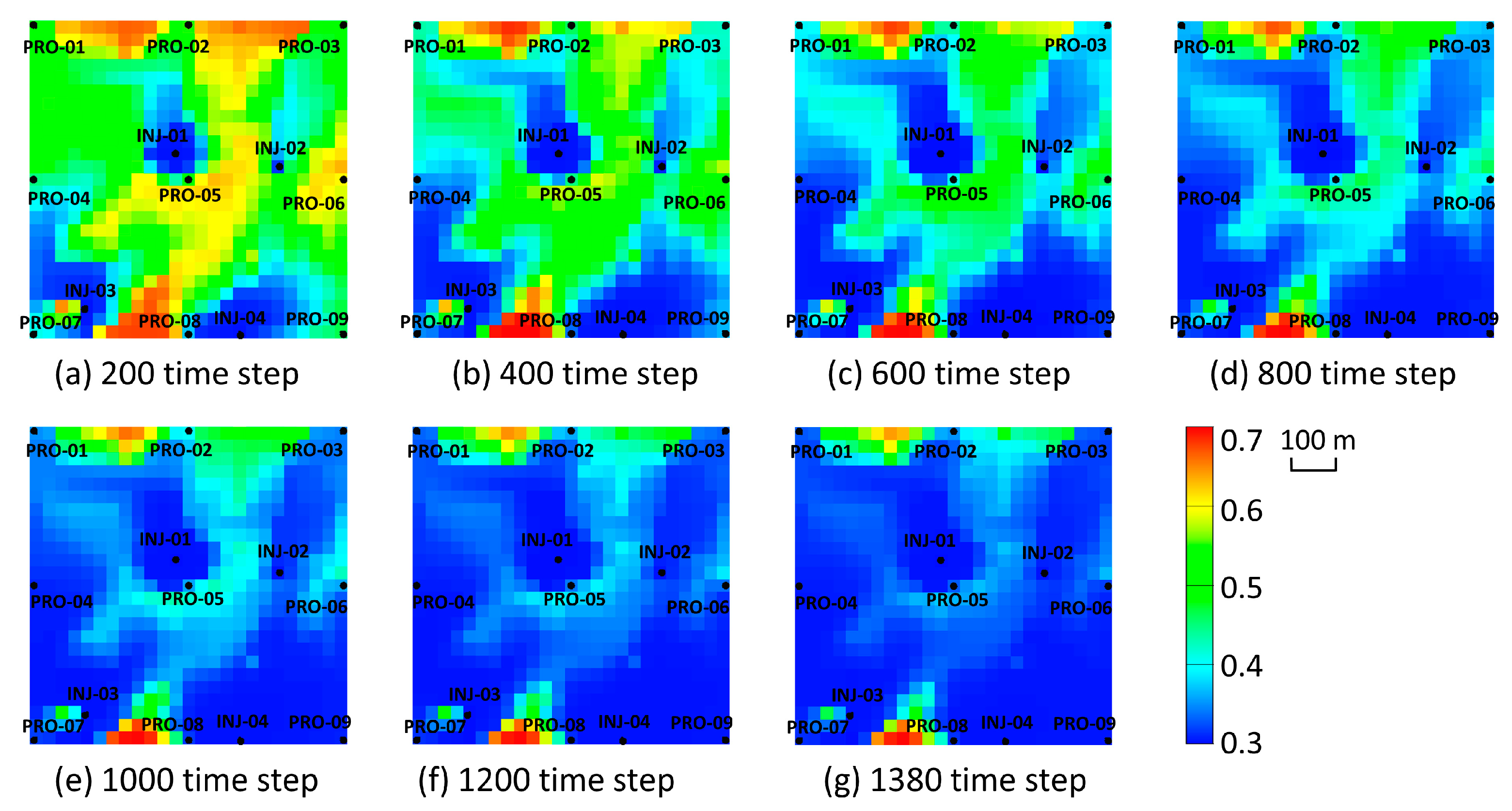
Figure 5a–g displays the oil saturation fields at different time steps of the three-channel case, from which we can observe the underground flow disequilibrium conditions. For instance, it is easy to find that the majority of the injected water of INJ-01 flows into PRO-01, and a small part flows into PRO-05. This is because there is a high-permeability area between INJ-01 and PRO-01, and the permeability distribution between INJ-01 and PRO-05 is very low, as shown in Figure 2. Hence, even PRO-05 is closer to INJ-01 than PRO-01, and the water is more likely to flow into the latter. A similar flow disequilibrium phenomenon can be found in INJ-02-PRO-03, since there is also a high-permeability area between this injector and producer. In addition, it is easier for the injected water of INJ-03 to displace the oil along the high-permeability channel to PRO-05 and PRO-04 than PRO-07, even though it is the nearest producer for INJ-03. Furthermore, there is no big difference in the permeability distribution between INJ-04-PRO-08 and INJ-04-PRO-09, so that the flow disequilibrium is not obvious between these two injector–producer groups.
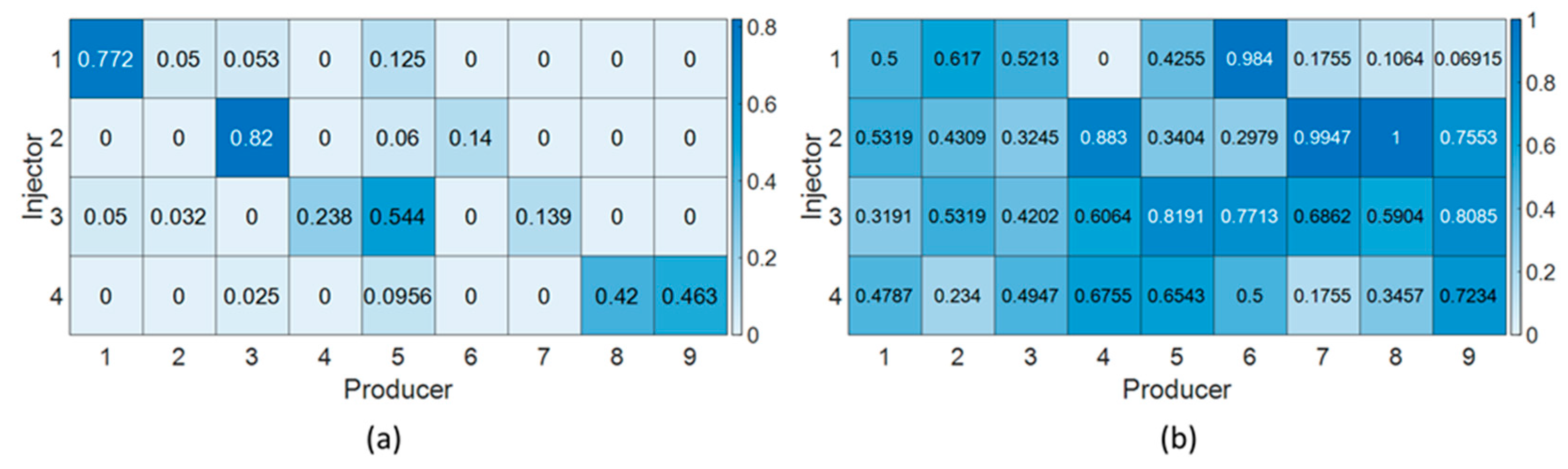
Based on the above analysis, we can test the performance of the proposed model and MLP on characterizing the inter-well flow disequilibrium. As shown in Figure 6a, the injector–producer groups located in the high-permeability area are successfully inferred via IRNN, where INJ01-PRO-01, INJ02-PRO-03, INJ03-PRO-05, INJ03-PRO-04 obtain the disequilibrium factors with 0.772, 0.82, 0.544, and 0.238, respectively. Additionally, INJ04-PRO-08 and INJ04-PRO-09, located on the homogeneous permeability area, are assigned to the values of 0.42 and 0.463 by IRNN, respectively. However, the disequilibrium factors computed by MLP cannot reflect the real inter-well flow distribution accurately. For example, the biggest disequilibrium factor of INJ-01 is assigned to INJ01-PRO-06 (0.984), which disagreed with the real oil saturation distribution in Figure 5. Moreover, the disequilibrium factor of INJ02-PRO-03 obtained via MLP is 0.3245, which is much smaller than the values of the following injector–producer groups: INJ02-PRO-08 (1.00), INJ02-PRO-07 (0.9947), and INJ02-PRO-04 (0.883), which are located in the low-permeability area. INJ03-PRO-05 is recognized by MLP, obtaining the disequilibrium factor with 0.8191, while the factors of INJ03-PRO-09 and INJ03-PRO-06 are 0.8085 and 0.7713, respectively, which is inconsistent with the permeability distribution shown in Figure 2 and the water driving process shown in Figure 5. In addition, MLP can characterize the connecting injector–producer pair INJ04-PRO-09 (with the factor of 0.7234), but the factor of INJ04-PRO-08 (0.3457) disagrees with the actual condition. Thus, the disequilibrium factors characterization results prove that IRNN is much more effective than the typical neural network in the quantitative analysis of the inter-well flow distribution, since the proposed model is integrated with the material balance equation and it takes account of the boundary constraint of the factors.
3.2. Olympus Model
The Olympus model is a benchmark reservoir model developed by TNO, inspired by an offshore oil field in the North Sea [25]. The Olympus field is three-dimensional, with 16 layers consisting of 192,750 active grids, and each grid is 50, 50, and 3 m in the x, y, and z axes, respectively. There are two zones in Olympus, where the top zone is a sedimentary environment of sandstone fluvial facies embedded in floodplain shales, and the bottom one consists of alternating layers of different grain size sands with a predetermined dip. Furthermore, there are 50 realizations of this model with different geological properties (permeability, porosity, initial oil saturation, and net-to-gross). We select realization 1 in this paper to test the performance of the proposed model. The Olympus model contains 11 producers and 7 injectors, producing around 7305 days (20 time steps). Figure 7 shows the permeability distribution of the Olympus model.
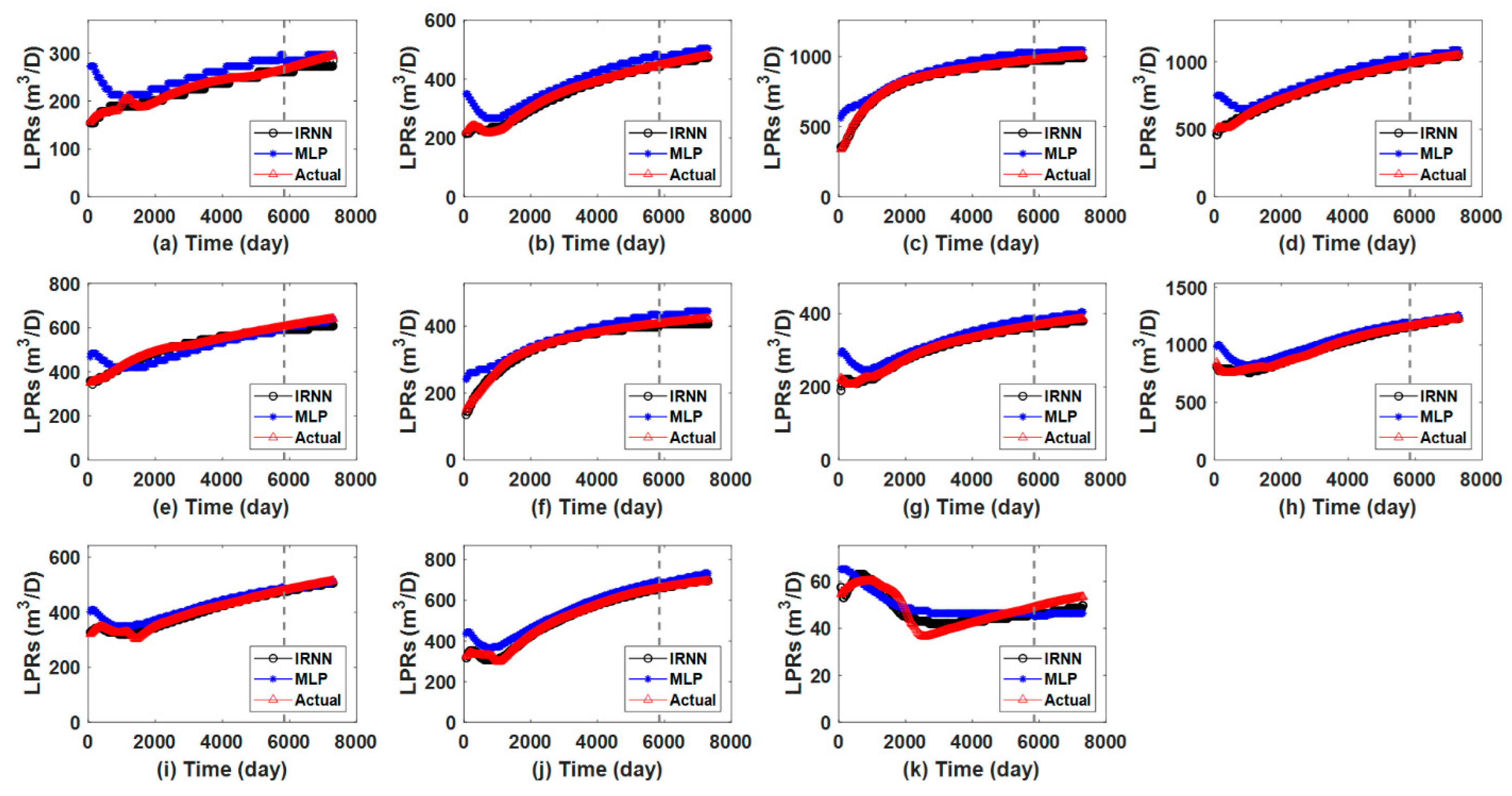
The estimated LPRs obtained via MLP and IRNN, and the observed LPRs generated by the simulator, are demonstrated in Figure 8. Different from the injection–production schedules in the three-channel model, there are no strong fluctuations in the injection and production signals in Olympus, and so the LPRs curves are much smoother than those in Figure 3. As expected, the proposed model shows a more powerful performance on the fitting and forecasting results of LPRs in the Olympus model. Specifically, as shown in Figure 8, in the early productivity fluctuating upward stage, MLP struggles to depict the details of the waves of LPRs, while the proposed model is capable of fitting the actual values with great accuracy. After that, during the stable increasing periods of LPRs, MLP provides a fair fitting and predicting result on the producers, except PRO-11, as shown in Figure 8k. In contrast with MLP, IRNN can match the history and predict the productivity behaviors of all producers with satisfactory accuracy. These results prove that the proposed model is effective for estimating and predicting productivity in complex heterogeneous reservoirs.
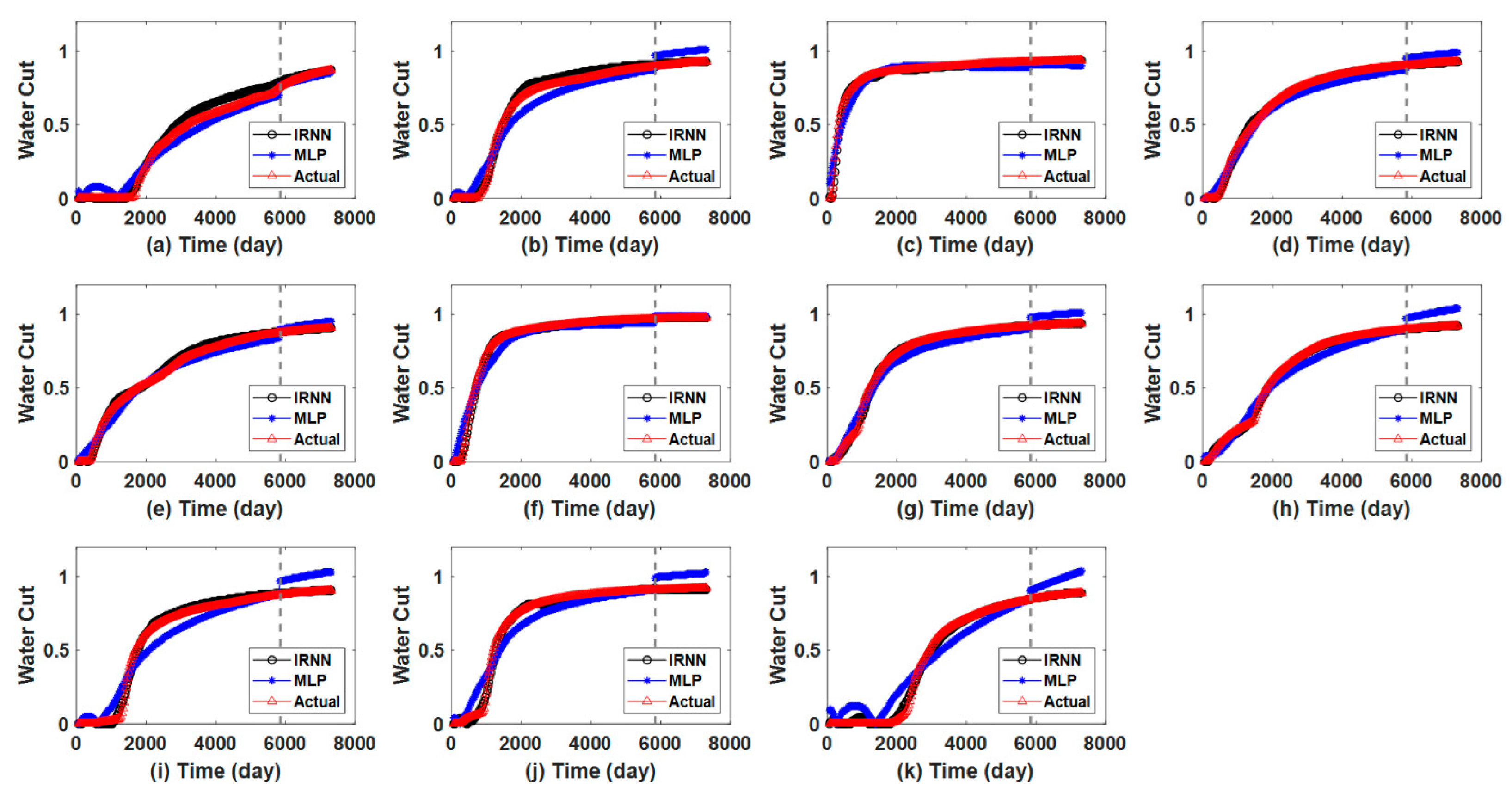
Figure 9 demonstrates the water cut curves modeled via MLP and IRNN, and the real curves provided by the simulator in the Olympus model. Generally, the main trend of the water cut curves can be fitted via MLP, while some details are not good. For instance, similar to the results of LPRs, there are some fluctuations of the water cut in the initial production startup stage, which cannot be accurately matched using MLP, as shown in Figure 9a,i–k. Furthermore, the performance of MLP on the forecast of the water cut curves is inconsistent with the true condition in Figure 9b,d,g–k, where the values obtained by MLP exceed 1. In contrast, the proposed model outperforms MLP on both the history matching and the prediction of the water cuts in all producers. The improvement of the performance of IRNN proves that the introduction of the material balance equation could effectively constrain the model outputs to within reasonable bounds, enhancing the robustness of IRNN. Furthermore, the recurrent neural network topology can help the model to significantly promote the ability to fit and to forecast a continuous time series.
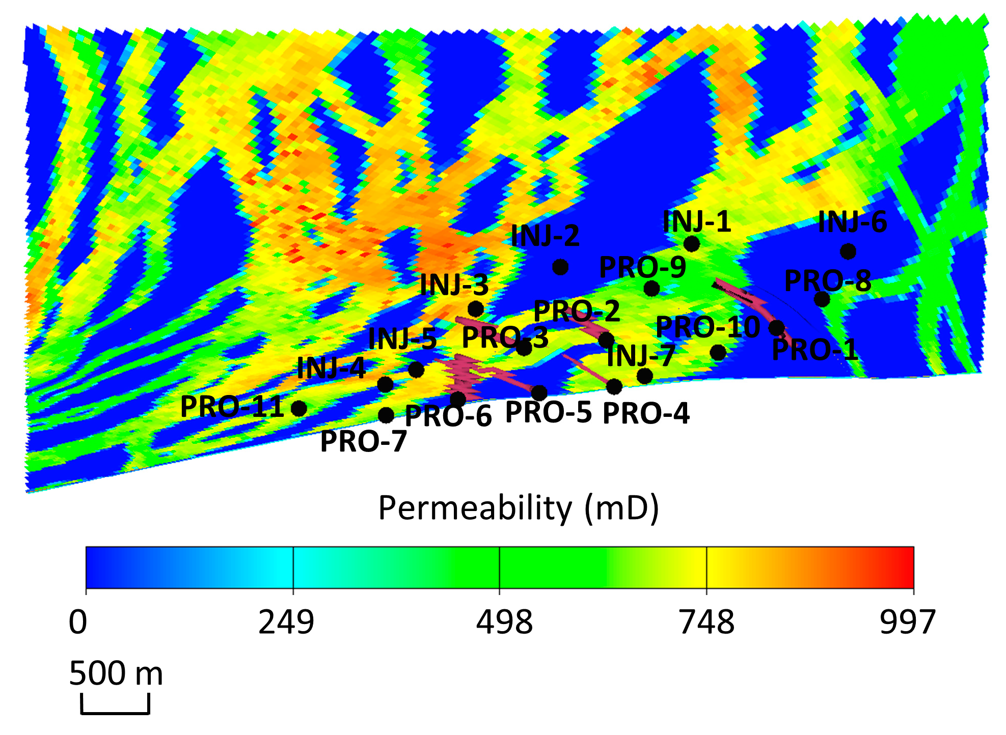
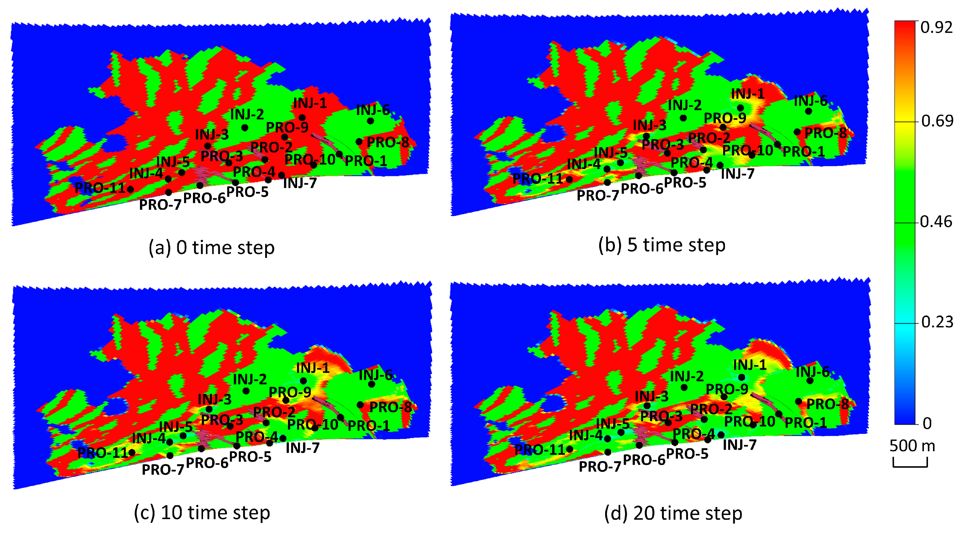
The oil saturation distribution at different time steps is demonstrated in Figure 10. As can be seen in Figure 7 and Figure 10, both the permeability and the initial oil saturation of the fluvial channels are high, so the injector–producer groups located in the channels can be considered to have strong connections, and the oil is easier to be driven by water than other low-permeability areas. As shown in Figure 10a–d, most of the injected water of INJ-1 flows to PRO-9, since this injector–producer pair is situated in the high-permeability channels, and the similar flow disequilibrium condition can be found in INJ-4-PRO-7, INJ-4-PRO-11, INJ-7-PRO-10, INJ-7-PRO-2, and INJ-7-PRO-4. Furthermore, the control volumes of the horizontal and deviated production wells are bigger than the vertical producers, and so their flow disequilibrium is influenced by the length and orientation of the well bores. For example, PRO-1 extends to the high-permeability area around INJ-1, so that the connectivity of this injector–producer pair would be strong, and so that similar strong connecting relationships can be found in INJ-3-PRO-3, INJ-5-PRO-5, and INJ-5-PRO-6. INJ-2 and INJ-6 are situated in the low-permeability area, as shown in Figure 7, so that the injected water of these two injectors would flow to the surrounding producers uniformly (PRO-2 and PRO-9 for INJ-2, and PRO-8 for INJ-6).
Table 4 lists the computation error and time of MLP and IRNN of the Olympus model. As expected, the proposed model outperforms MLP on both the history matching and forecast of the production behaviors. In terms of LPRs, the history matching and prediction errors of IRNN are 0.0066 and 1.4986 × 10⁻⁴, which are only 24.26% and 3.12% of those obtained via MLP. In addition, the history matching and prediction errors of the water cut of IRNN (0.0012 and 1.4271 × 10⁻⁴, respectively) are more than one order of magnitude lower than those of MLP (0.0137 and 0.0054, respectively). As listed in Table 4, although MLP costs less computation time (3.9843 s for LPRs and 3.0625 s for water cut) than IRNN, the proposed model can finish the calculation within tens of seconds. Therefore, at the cost of an acceptable increase in the calculation time, both the fitting and the prediction abilities of IRNN are significantly enhanced.
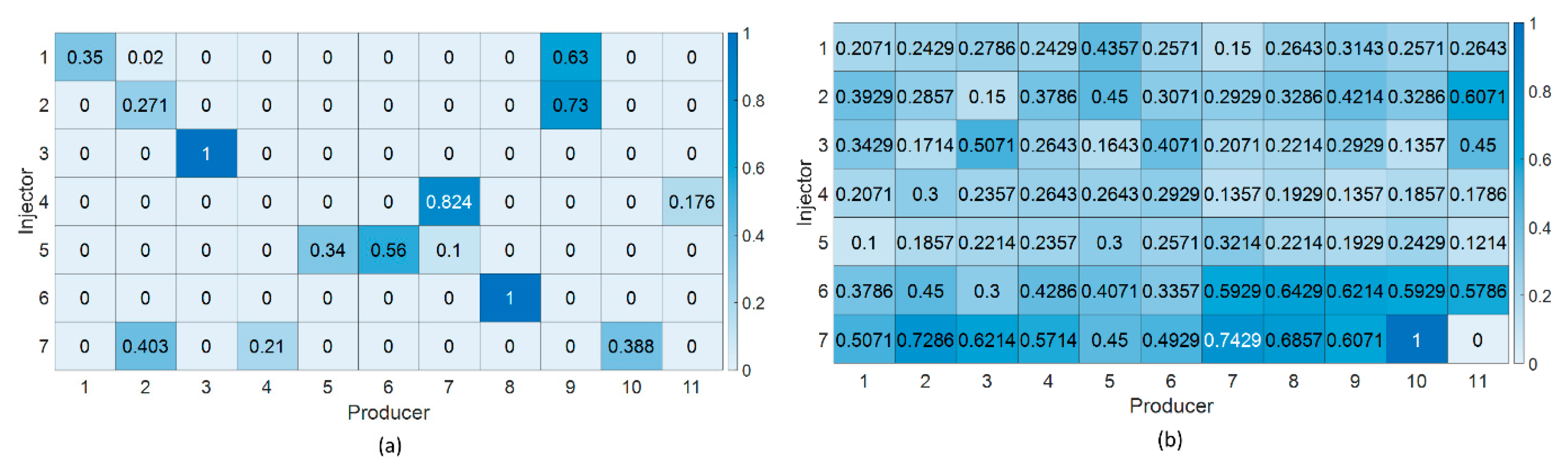
Figure 11 demonstrates the disequilibrium factors of the Olympus model calculated via IRNN and MLP. As shown in Figure 11a, the injector–producer pairs located in the high-permeability fluvial channels, such as INJ-1-PRO-9, INJ-4-PRO-7, INJ-4-PRO-11, INJ-7-PRO-10, INJ-7-PRO-2, and INJ-7-PRO-4 are characterized correctly via IRNN, obtaining the factors with 0.63, 0.824, 0.176, 0.388, 0.403, and 0.21, respectively. In addition, the injector–producer groups containing the horizontal or deviated production wells as discussed above, are also recognized successfully via IRNN, where INJ-1-PRO-1, INJ-3-PRO-3, INJ-5-PRO-5, and INJ-5-PRO-6 are assigned to the disequilibrium factors of 0.35, 1, 0.34, and 0.56 by IRNN, respectively. Furthermore, INJ-2-PRO-2, INJ-2-PRO-9, and INJ-6-PRO-8 with close well-distance, are also inferred accurately by IRNN, with the factors of 0.271, 0.73, and 1, respectively. However, as shown in Figure 11b, MLP only recognizes the strong connecting well pairs of INJ-3-PRO-3, INJ-5-PRO-5, INJ-6-PRO-8, and INJ-7-PRO-10, which obtain the factors of 0.5071, 0.3, 0.6429, and 1, respectively. Meanwhile, many injector–producer pairs that are located in the low-permeability areas are endowed with big disequilibrium factors, such as INJ-1-PRO-5 (0.4357), INJ-2-PRO-5 (0.45), INJ-6-PRO-7 (0.5929), and INJ-7-PRO-7 (0.7429). The disequilibrium factors calculated using MLP are not as sparse as the results obtained using IRNN, because there is no seepage-physics-knowledge (including the boundary constraint) in the development of MLP, leading to the fact that the characterization results cannot reflect the actual injection volume fractions accurately. In summary, IRNN demonstrates a better performance than MLP on the flow disequilibrium analysis of the Olympus model, proving the effectiveness of the physics-knowledge embedded learning framework.
4. Conclusions
In this paper, we propose an interpretable recurrent neural network (IRNN) to simulate the production behaviors, and to characterize the inter-well flow disequilibrium in waterflooding reservoirs, only using water injection rates and bottom hole pressure data. IRNN is established on the material balance equation, and thus, the seepage-physics-knowledge can be used to guide the learning process. IRNN consists of an inflow module and a drainage module, where the inflow module aims to compute the total water injection rates from all injectors to each producer, and the drainage module is used to estimate the fluid change rate among the water drainage volume. On the temporal scale, to improve the utilization efficiency of the historical information, the gated recurrent unit (GRU) block is employed in IRNN, so that the important historical injection–production data can be memorized. Furthermore, IRNN adopts the self-attention block to focus on the important injection–production signals, and to reduce the influence of useless information, so that the proposed model can capture the hydrodynamic characteristics on the spatial scale of the reservoir. Moreover, inspired by the work of feature selection, a Gaussian kernel function is introduced in IRNN to quantitatively measure the flow disequilibrium for each injector–producer group. Meanwhile, the boundary constraint of the disequilibrium factors is considered in the loss function of IRNN, to guarantee the rationality of the characterization results. The proposed model outperforms the classical neural network (MLP) on both the history matching and the prediction of production behaviors (including LPRs and water cut), and the analysis of inter-well flow disequilibrium on two synthetic reservoir models. Therefore, we believe that the proposed model provides a new way to integrate the seepage-physics-knowledge and the machine learning model, which is very valuable for improving the accuracy, interpretability, and robustness of the machine learning methods. In the future, we would like to use the proposed model to deal with other problems of waterflooding reservoirs, such as production optimization.
Author Contributions
Conceptualization, Y.J. and K.Z.; methodology, J.W. and H.Z.; software, Y.J. and H.Z.; validation, W.S.; formal analysis, Y.J. and W.S.; investigation, Y.J.; resources, K.Z. and L.Z.; data curation, Y.J. and W.S.; writing—original draft preparation, Y.J.; writing—review and editing, Y.J. and K.Z.; visualization, Y.J.; supervision, K.Z. and J.W.; project administration, K.Z.; funding acquisition, K.Z. All authors have read and agreed to the published version of the manuscript.
Funding
This work is supported by the National Natural Science Foundation of China under Grants 52274057, 52074340, and 51874335, the Major Scientific and Technological Projects of CNPC under Grant ZD2019-183-008, the Major Scientific and Technological Projects of CNOOC under Grant CCL2022RCPS0397RSN, the Science and Technology Support Plan for Youth Innovation of University in Shandong Province under Grant 2019KJH002, and 111 Project under Grant B08028.
Institutional Review Board Statement
Not applicable.
Informed Consent Statement
Not applicable.
Data Availability Statement
The data used in this paper are not publicly available due to limitations of consent for the original study, but they could be obtained from Dr. Jiang upon reasonable request.
Conflicts of Interest
The authors declare no conflict of interest. The funders had no role in the design of the study; in the collection, analyses, or interpretation of data; in the writing of the manuscript, or in the decision to publish the results.
References
- Xu, J.; Zhan, S.; Wang, W.; Su, Y.; Wang, H. Molecular dynamics simulations of two-phase flow of n-alkanes with water in quartz nanopores. Chem. Eng. J. 2022, 430, 132800. [Google Scholar] [CrossRef]
- Li, W.; Nan, Y.; Wen, X.; Wang, W.; Jin, Z. Effects of Salinity and N-, S-, and O-Bearing Polar Components on Light Oil–Brine Interfacial Properties from Molecular Perspectives. J. Phys. Chem. C 2019, 123, 23520–23528. [Google Scholar] [CrossRef]
- Sheng, G.; Su, Y.; Wang, W. A new fractal approach for describing induced-fracture porosity/permeability/ compressibility in stimulated unconventional reservoirs. J. Pet. Sci. Eng. 2019, 179, 855–866. [Google Scholar] [CrossRef]
- Wang, W.; Fan, D.; Sheng, G.; Chen, Z.; Su, Y. A review of analytical and semi-analytical fluid flow models for ultra-tight hydrocarbon reservoirs. Fuel 2019, 256, 115737. [Google Scholar] [CrossRef]
- Cai, J.; Jin, T.; Kou, J.; Zou, S.; Xiao, J.; Meng, Q. Lucas–Washburn Equation-Based Modeling of Capillary-Driven Flow in Porous Systems. Langmuir 2021, 37, 1623–1636. [Google Scholar] [CrossRef]
- Chen, G.; Li, Y.; Zhang, K.; Xue, X.; Wang, J.; Luo, Q.; Yao, C.; Yao, J. Efficient hierarchical surrogate-assisted differential evolution for high-dimensional expensive optimization. Inf. Sci. 2021, 542, 228–246. [Google Scholar] [CrossRef]
- Yousef, A.A.; Gentil, P.H.; Jensen, J.L.; Lake, L.W. A Capacitance Model To Infer Interwell Connectivity From Production and Injection Rate Fluctuations. SPE Reserv. Eval. Eng. 2006, 9, 630–646. [Google Scholar] [CrossRef]
- Naudomsup, N.; Lake, L.W. Extension of Capacitance/Resistance Model to Tracer Flow for Determining Reservoir Properties. SPE Reserv. Eval. Eng. 2018, 22, 266–281. [Google Scholar] [CrossRef]
- Temizel, C.; Artun, E.; Yang, Z. Improving Oil-Rate Estimate in Capacitance/Resistance Modeling Using the Y-Function Method for Reservoirs Under Waterflood. SPE Reserv. Eval. Eng. 2019, 22, 1161–1171. [Google Scholar] [CrossRef]
- Gubanova, A.; Orlov, D.; Koroteev, D.; Shmidt, S. Proxy Capacitance-Resistance Modeling for Well Production Forecasts in Case of Well Treatments. SPE J. 2022, 27, 3474–3488. [Google Scholar] [CrossRef]
- Arouri, Y.; Lake, L.W.; Sayyafzadeh, M. Bilevel Optimization of Well Placement and Control Settings Assisted by Capacitance-Resistance Models. SPE J. 2022, 27, 3829–3848. [Google Scholar] [CrossRef]
- Zhao, H.; Kang, Z.; Zhang, X.; Sun, H.; Cao, L.; Reynolds, A.C. INSIM: A Data-Driven Model for History Matching and Prediction for Waterflooding Monitoring and Management with a Field Application. In Proceedings of the SPE Reservoir Simulation Symposium, Houston, TX, USA, 23 February 2015. [Google Scholar]
- Guo, Z.; Chen, C.; Gao, G.; Vink, J. Enhancing the Performance of the Distributed Gauss-Newton Optimization Method by Reducing the Effect of Numerical Noise and Truncation Error With Support-Vector Regression. SPE J. 2018, 23, 2428–2443. [Google Scholar] [CrossRef]
- Zhang, Y.; He, J.; Yang, C.; Xie, J.; Fitzmorris, R.; Wen, X.-H. A Physics-Based Data-Driven Model for History Matching, Prediction, and Characterization of Unconventional Reservoirs. SPE J. 2018, 23, 1105–1125. [Google Scholar] [CrossRef]
- Guo, Z.; Reynolds, A.C. INSIM-FT-3D: A Three-Dimensional Data-Driven Model for History Matching and Waterflooding Optimization. In Proceedings of the SPE Reservoir Simulation Conference, Society of Petroleum Engineers, Galveston, TX, USA, 20–22 February 2019; p. SPE–193841-MS. [Google Scholar]
- Li, Y.; Onur, M. INSIM-BHP: A physics-based data-driven reservoir model for history matching and forecasting with bottomhole pressure and production rate data under waterflooding. J. Comput. Phys. 2023, 473, 111714. [Google Scholar] [CrossRef]
- Artun, E. Characterizing interwell connectivity in waterflooded reservoirs using data-driven and reduced-physics models: A comparative study. Neural Comput. Appl. 2017, 28, 1729–1743. [Google Scholar] [CrossRef]
- Jensen, J. Comment on “Characterizing interwell connectivity in waterflooded reservoirs using data-driven and reduced-physics models: A comparative study” by E. Artun DOI 10.1007/s00521-015-2152-0. Neural Comput. Appl. 2016, 28, 1–2. [Google Scholar] [CrossRef]
- Mo, S.; Zhu, Y.; Zabaras, N.; Shi, X.; Wu, J. Deep Convolutional Encoder-Decoder Networks for Uncertainty Quantification of Dynamic Multiphase Flow in Heterogeneous Media. Water Resour. Res. 2019, 55, 703–728. [Google Scholar] [CrossRef]
- Carpenter, C. Machine Learning Improves Accuracy of Virtual Flowmetering and Back-Allocation. J. Pet. Technol. 2019, 71, 77–78. [Google Scholar] [CrossRef]
- Zhang, Z.; He, X.; AlSinan, M.; Kwak, H.; Hoteit, H. Robust Method for Reservoir Simulation History Matching Using Bayesian Inversion and Long-Short-Term Memory Network-Based Proxy. SPE J. 2022, 1–25. [Google Scholar] [CrossRef]
- Chakraborty, R.; Pal, N.R. Feature Selection Using a Neural Framework With Controlled Redundancy. IEEE Trans. Neural Netw. Learn. Syst. 2015, 26, 35–50. [Google Scholar] [CrossRef]
- Chen, G.; Zhang, K.; Xue, X.; Zhang, L.; Yao, J.; Sun, H.; Fan, L.; Yang, Y. Surrogate-assisted evolutionary algorithm with dimensionality reduction method for water flooding production optimization. J. Pet. Sci. Eng. 2020, 185, 106633. [Google Scholar] [CrossRef]
- Chen, G.; Zhang, K.; Zhang, L.; Xue, X.; Ji, D.; Yao, C.; Yao, J.; Yang, Y. Global and Local Surrogate-Model-Assisted Differential Evolution for Waterflooding Production Optimization. SPE J. 2020, 25, 105–118. [Google Scholar] [CrossRef]
- Fonseca, R.-M.; Rossa, E.; Emerick, A.; Hanea, R.G.; Jansen, J.-D. Overview Of The Olympus Field Development Optimization Challenge. In Proceedings of the 16th European Conference on the Mathematics of Oil Recovery, ECMOR 2018, Barcelona, Spain, 3–6 September 2018. [Google Scholar]
Figure 1.
The architecture of the interpretable recurrent neural network.

Figure 2.
Permeability distribution of the three-channel model.

Figure 3.
The liquid production rate curves of the three-channel model. The red lines with triangles represent the actual results obtained by the simulator, the black lines with circles represent the results obtained via IRNN, and the blue lines with dots are the results obtained via MLP. The history matching and predicting periods are divided by the grey vertical dashed line. From PRO-01 to PRO-09, the liquid production rates of 9 producers are demonstrated in (a–i) successively.

Figure 4.
The water cut curves of the three-channel model. The red lines with triangles represent the actual results obtained by the simulator, the black lines with circles represent the results obtained via IRNN, and the blue lines with dots are the results obtained via MLP. The history matching and predicting periods are divided by the grey vertical dashed line. From PRO-01 to PRO-09, the water cut curves of 9 producers are demonstrated in (a–i) successively.

Figure 5.
The oil saturation distribution at different time steps of the three-channel model.

Figure 6.
The disequilibrium factors of the three-channel model. (a): The results obtained via IRNN; (b) The results obtained via MLP.
Figure 6.
The disequilibrium factors of the three-channel model. (a): The results obtained via IRNN; (b) The results obtained via MLP.

Figure 7.
Permeability distribution of Olympus model.

Figure 8.
The liquid production rate curves of Olympus model. The red lines with triangles represent the actual results obtained by the simulator, the black lines with circles represent the results obtained via IRNN, and the blue lines with dots are the results obtained via MLP. The history matching and predicting periods are divided by the grey vertical dashed line. From PRO-1 to PRO-11, the liquid production rates of 11 producers are demonstrated in (a–k) successively.

Figure 9.
The water cut curves of the Olympus model. The red lines with triangles represent the actual results obtained by the simulator, the black lines with circles represent the results obtained via IRNN, and the blue lines with dots are the results obtained via MLP. The history matching and predicting periods are divided by the grey vertical dashed line. From PRO-1 to PRO-11, the water cut curves of 11 producers are demonstrated in (a–k) successively.

Figure 10.
The oil saturation distribution at different time steps of Olympus model.

Figure 11.
The disequilibrium factors of Olympus model. (a): The results obtained via IRNN; (b) The results obtained via MLP.
Figure 11.
The disequilibrium factors of Olympus model. (a): The results obtained via IRNN; (b) The results obtained via MLP.


Table 1.
The hyperparameters used in IRNN.
| Hyperparameter | IRNN |
|---|---|
| Hidden nodes of GRU block | 15 |
| Hidden nodes of queries, keys, and values of self-attention block | 10 |
| Hidden nodes of fully connected layer | 15 |
| Batch size | 10 |
| Initial learning rate | 0.03 |
| Coefficient of regularization item | 0.02 |
Table 2.
Geological properties of the three-channel model.
| Reservoir Properties | Values |
|---|---|
| Model scale | 25 × 25 × 1 |
| Grid size | 100 × 100 × 10 ft |
| Depth | 4800 ft |
| Initial pressure | 4000 psi |
| Initial temperature | 100 °C |
| Pore compressibility | 6.9 × 10⁻⁵ psi−1 |
| Porosity | 0.20 |
| Initial oil saturation | 0.80 |
| Oil density | 900 kg/m3 |
| Oil viscosity | 2.2 cP |
| Water density | 1000 kg/m3 |
| Water viscosity | 0.5 cP |
Table 3.
The computation error (MSE) and time (seconds) of both MLP and IRNN of the three-channel model.
Table 3.
The computation error (MSE) and time (seconds) of both MLP and IRNN of the three-channel model.
| MLP | IRNN | |
|---|---|---|
| History matching error of LPRs | 0.0933 | 0.0124 |
| Prediction error of LPRs | 0.2465 | 0.0203 |
| History matching error of water cut | 0.0242 | 0.0017 |
| Prediction error of water cut | 0.0225 | 4.9051 × 10⁻⁴ |
| Training time of LPRs | 24.1563 s | 208.9531 s |
| Training time of water cut | 16.3875 s | 170.5313 s |
Table 4.
The computation error (MSE) and time (seconds) of both MLP and IRNN of Olympus model.
| MLP | IRNN | |
|---|---|---|
| History matching error of LPRs | 0.0272 | 0.0066 |
| Prediction error of LPRs | 0.0320 | 1.4986 × 10⁻⁴ |
| History matching error of water cut | 0.0137 | 0.0012 |
| Prediction error of water cut | 0.0054 | 1.4271 × 10⁻⁴ |
| Training time of LPRs | 3.9843 s | 71.5156 s |
| Training time of water cut | 3.0625 s | 64.9062 s |
Disclaimer/Publisher’s Note: The statements, opinions and data contained in all publications are solely those of the individual author(s) and contributor(s) and not of MDPI and/or the editor(s). MDPI and/or the editor(s) disclaim responsibility for any injury to people or property resulting from any ideas, methods, instructions or products referred to in the content. |
© 2023 by the authors. Licensee MDPI, Basel, Switzerland. This article is an open access article distributed under the terms and conditions of the Creative Commons Attribution (CC BY) license (https://creativecommons.org/licenses/by/4.0/).
Share and Cite
MDPI and ACS Style
Jiang, Y.; Shen, W.; Zhang, H.; Zhang, K.; Wang, J.; Zhang, L. An Interpretable Recurrent Neural Network for Waterflooding Reservoir Flow Disequilibrium Analysis. Water 2023, 15, 623. https://doi.org/10.3390/w15040623
AMA Style
Jiang Y, Shen W, Zhang H, Zhang K, Wang J, Zhang L. An Interpretable Recurrent Neural Network for Waterflooding Reservoir Flow Disequilibrium Analysis. Water. 2023; 15(4):623. https://doi.org/10.3390/w15040623
Chicago/Turabian StyleJiang, Yunqi, Wenjuan Shen, Huaqing Zhang, Kai Zhang, Jian Wang, and Liming Zhang. 2023. "An Interpretable Recurrent Neural Network for Waterflooding Reservoir Flow Disequilibrium Analysis" Water 15, no. 4: 623. https://doi.org/10.3390/w15040623
Note that from the first issue of 2016, this journal uses article numbers instead of page numbers. See further details here.