

A Combined Stochastic–Analytical Method for the Assessment of Climate Change Impact on Spring Discharge

1
Institute of Environmental Management, University of Miskolc, H-3515 Miskolc-Egyetemváros, 3515 Miskolc, Hungary
2
National Laboratory for Water Science and Water Security, University of Miskolc, H-3515 Miskolc-Egyetemváros, 3515 Miskolc, Hungary
3
Centre for Karst Hydrogeology, Faculty of Mining & Geology, University of Belgrade, Djušina 7, 11000 Belgrade, Serbia
*
Author to whom correspondence should be addressed.
Water 2023, 15(4), 629; https://doi.org/10.3390/w15040629
Submission received: 13 December 2022
/
Revised: 30 January 2023
/
Accepted: 2 February 2023
/
Published: 6 February 2023
(This article belongs to the Special Issue Hydrogeology and Geochemistry of Karst Aquifers)
Abstract
:This study describes a novel methodology for the prediction of spring hydrographs based on regional climate model (RCM) projections, with the goal of evaluating climate-change impact on karstic-spring discharge. A combined stochastic–analytical modeling methodology to predict spring discharge was developed and demonstrated on the Bukovica spring catchment at the Durmitor National Park, Montenegro. As a first step, climate model projections of the EURO-CORDEX ensemble were selected; and then bias correction was applied based on historical climate data. The regression function between rainfall and peak discharge was established by using historical data. Baseflow recession was described by using a double-component exponential model, where hydrograph decomposition and parameter fitting were performed on the Master Recession Curve. Rainfall time series from two selected RCM scenarios were applied to predict future spring-discharge time series. Bias correction of simulated hydrographs was performed, and bias-corrected combined stochastic–analytical models were applied to predict spring hydrographs based on RCM-simulated rainfall data. Both simulated climate scenarios predict increasing peak discharges and decreasing baseflow discharges throughout the 21st century. The model results suggest that climate change is likely to exaggerate the extremities both in terms of climate parameters and spring discharge by the end of the century both for moderate (RCP 45) and pessimistic (RCP 85) CO2 emission scenarios. To investigate the temporal distribution of extremities throughout the simulated time periods, the annual numbers of flood and drought days were calculated. Annual predicted flood days show an increasing trend during the first simulation period (2021–2050) and a slightly decreasing trend during the second simulation period (2071–2100), according to the RCP45 climate scenario. The same parameter shows a stagnant trend for the RCP 85 climate scenario. Annual predicted drought days show a decreasing trend both for the RCP 45 and RCP 85 climate scenarios. However, the annual number of drought days shows a large variation over time. There is a periodicity of extremely dry years with a frequency between 5 and 7 years. The number of drought days seems to increase over time during these extreme years. The study confirmed that the applied methodology can successfully be applied for spring-discharge prediction and that it offers a new prospect for its wider application in studying karst aquifers and their behavior under different climate-change scenarios.
1. Introduction
Karst aquifers represent one of the globally most important sources for potable water supply. According to Stevanović [1], around 9.2% of the human population drinks karst water. In certain countries of Southeast Europe, which are mainly occupied by carbonate rocks, such as Slovenia or Austria, more than 50% of the total water consumption is supplied from karst aquifers. Montenegro has the highest utilization of karst water, with 80% of its territory occupied by uncovered carbonate karst [2] and about 90% of the population using karst water for drinking purposes [1]. However, even there, extended dry periods might result in the decrease or cessation of spring discharge and thus endanger the continuity of water supply which is based on karst water [3].
In the meanwhile, karst springs are not only important sources of water; they also represent a significant risk to the human population. Flash floods are unforeseen surges of spring water that often endanger the built environment and human life, and bacterial epidemics related to the rapid transport of contaminants in karst conduits during flood events represent significant health risks.
According to the climate projections of the Intergovernmental Panel on Climate Change (IPCC), significant temperature rise, together with alterations in the amount and frequency of precipitation, can be expected globally throughout the rest of the 21st century [4,5,6].
Climate change (CC) results in changes in the intensity, frequency, spatial extent, duration, and timing of extreme climate events, and it can cause unprecedented extreme events [7]. The observations gathered since 1950 prove the change in some extremes and that these changes result from anthropogenic influences, such as the increases in atmospheric greenhouse-gas concentrations.
Some of the greenhouse-gas-emission scenarios initially developed by the IPCC [5] commonly make climate projections by manipulating general circulation models/global climate models (GCMs), as was achieved in projects such as PRUDENCE [8], ENSEMBLES [9], or CORDEX [10]. However, there is no single CC scenario that is appropriate for all circumstances. The applied scenario should be chosen according to context and local conditions, while the accuracy of models depends on the grid scale and the ability to understand and measure climate processes [11].
Since the 1950s, a trend toward more intense and longer droughts has been experienced in some regions of the world. Because of reduced precipitation and/or increased evapotranspiration, droughts are predicted to intensify in the 21st century in many areas according to all model predictions. It is also expected that the frequency of heavy rainfall events will increase in the 21st century over many areas of the globe. This is especially the case at high latitudes and tropical regions, as well as during winter in the northern mid-latitudes. The intensity of tropical cyclones with heavy rainfalls is expected to increase with the continued warming resulting from greenhouse gas emissions. In some regions, such as parts of the Mediterranean Basin, despite the projected decrease in total precipitation, the intensity of heavy rainfall will increase [12].
Changing climate variables influence the hydrological cycle by impacting the surface runoff, evapotranspiration, and recharge of aquifer systems [13]. In the case of karst aquifers, spring discharge strongly correlated with rainfall. For this reason, climate change has direct impacts on water supplies based on karst springs [14].
The goal of the present paper is to outline a methodology for the prediction of spring-discharge time series based on forecasted-rainfall time series that were derived from regional climate model projections. For this purpose, a combined stochastic–analytical modeling approach was developed. The study aimed at modeling the direct impacts of climate change on spring hydrographs; it did not aim at simulating indirect impacts, such as increased groundwater extraction, land-use change, etc. The introduced methodology is demonstrated in the Dinaric karst, using the Bukovica spring catchment of the Drina River Basin, Šavnik municipality, Montenegro, as the example. This area is characterized by a high karstification rate, abundance of surface karst features, and the lack of surface hydrographic network. The Bukovica spring catchment belongs to the Durmitor national park, comprising the Tara River canyon, the deepest canyon in Europe, which is a UNESCO protected reserve.
The methodology presented in this article was developed during a regional study [15] that aimed to assess the impact of CC on this important natural reservation area and karst aquifer, which is the main water source for entire region. As the primary goal of this paper was to develop and demonstrate a methodology, only a limited set of climate model scenarios were investigated.
2. Precedents
Various authors have attempted to develop a mathematical characterization of spring hydrographs to provide spring-discharge predictions. These methods can be classified based on the investigated hydrograph duration and the representation of the physical processes behind the functioning of karst systems.
Time-series analyses investigate the hydrograph of a karst system during a succession of recharge events. These methods are based on mathematical operations, and their results cannot be directly related to physical characteristics. On the other hand, these methods can deal with long time series and have the ability for characterizing uncertainty related to the spatiotemporal heterogeneity of rainfall, recharge, and aquifer properties. Most of the methods used in time-series analysis were principally developed by Jenkins and Watts [16] and some later works. These investigations mainly focused on forecasting and data completion. The application of time-series analyses to the description of the functioning of karst aquifers first appeared in Mangin [17,18,19,20]. Some further applications of these methods were presented in [21,22,23,24,25]. Amongst others, Fiorillo et al. [26] performed statistical and specific correlation data analyses to establish the relationship between spring discharge and rainfall. Fiorillo and Doglioni [27] investigated the relation between rainfall and the discharge from two springs located at the base of different karst massifs in Southern Italy by cross-correlation analyses, for example.
Reservoir or ‘bucket’ models can provide simple input–output relationships between rainfall and spring discharge. Spring hydrographs are traditionally simulated by using reservoir models. The simplest model configuration includes two reservoirs: the first reservoir represents the low-permeability matrix discharging into the conduit system, while the second reservoir represents the high-permeability conduit system [28]. Several other components can be added, and reservoir configurations can be applied to better simulate the infiltration process and to obtain a better fit to spring discharge, as described in [29,30,31,32,33,34] and several other studies.
Analytical methods can be applied for obtaining quantitative information about the hydraulic and geometric properties of karst aquifers. The one-dimensional analytical solutions [35,36] and the two-dimensional analytical solutions provided by Kovács [37,38] showed that the recession coefficient (α) is proportional to the ratio T/SL2 where L is block size [L], T is the hydraulic transmissivity [L2T−1], and S is the storativity [-] of the rock matrix. The work of these authors made the estimation of conduit spacing and rock matrix hydraulic properties possible from hydrograph analysis.
Artificial neural networks (ANNs) or their subgroup of deep learning (DL) approaches offer an alternative possibility of modeling by being able to establish an input–output relationship automatically. The advantage of the ANN is that it does not necessitate a priori knowledge about the system it represents and is able to implement nonlinearity. A particular model called the multilayer perceptron can approximate any derivable function [39,40]. In hydrology, neural networks have been shown to be effective for the identification of rainfall–discharge (or water level) relation prediction applications [41,42,43,44]. In examining karst system modeling more specifically, the effectiveness of such models in simulating and short-term forecasting karst outlet discharge has also been proven [45,46]. However, more recent works have focused on the ability to interpret these models with actual physical meaning [47]. In the study of Kong-A-Siou et al. [48], rainfall-water-level models were proposed in addition to rainfall–discharge models.
As detailed above, several different methods have been developed and applied for the prediction of spring discharge. Each has its advantages and shortcomings. The main motivation for developing a new method was to integrate the advantage of stochastic methods of being able to deal with the spatial and temporal variability of rainfall with the advantage of analytical models of providing a physics-based description of flow processes.
3. Materials and Methods
3.1. Hydrograph Features
The plots of spring discharge versus time are referred to as spring hydrographs. Hydrographs consist of a succession of individual peaks, each of which represents the response of the aquifer given to a recharge event (Figure 1). Each hydrograph peak consists of a rising and a falling limb. The inflection point on the falling limb indicates the end of direct recharge. The steep segment before the inflection point is called the flood recession, while the flat segment after the inflection point is referred to as the baseflow recession. Quickflow originates from direct recharge through sinkholes and vertical shafts collecting water from sinking streams and from the epikarst. This component of hydrograph peaks is influenced by the topography, land use, soil and epikarst characteristics, and depth of the saturated zone. These properties might influence the proportion, temporal distribution, and temporal delay of quickflow compared to rainfall. Baseflow originates from water released from the low-permeability matrix blocks and is much less influenced by the temporal and spatial variations of rainfall than quickflow. The recharge of matrix blocks takes place through diffuse infiltration from the surface and through gradient inversion between the blocks and neighboring conduits (bank storage) [28].
3.2. Hydrograph Analysis
The first mathematical models of baseflow recession were provided by Boussinesq and later by Maillet [35,49]:
where Qt is the discharge [L3T−1] at time t; Q0 is the initial discharge [L3T−1] at an earlier time; and α is the recession coefficient [T−1], which is usually expressed in days. Plotted on a semi-logarithmic graph, this function is represented as a straight line with the slope α. This equation is usually adequate for describing karst systems at low water stages.
The earlier stages of baseflow recession usually deviate from the simple exponential formulaof Maillet [49]. Forkasiewitz and Paloc [50] realized that the decreasing limb of hydrograph peaks can usually be decomposed into several (usually three) exponential segments. These authors introduced the concept of hydrograph decomposition. During decomposition, exponential terms are fitted on the flattest section of a spring hydrograph and are successively subtracted from the residual hydrograph (Figure 2).
Forkasiewitz and Paloc [50] assumed that different segments of a spring hydrograph peak represent different parallel reservoirs, all contributing to the discharge of the spring.
Schoeller [51] assumed that successive exponential decreasing limbs on spring hydrographs are due to changes of flow regimes (from turbulent to laminar).
Kovács [37,38] provided an exact analytical solution to baseflow, and Kovács and Perrochet [52] showed that baseflow recession can be described as a sum of infinite number of exponential components:
These authors demonstrated that exponential components usually do not represent different permeability classes; instead, they are the consequence of transient phenomena during the emptying of low permeability matrix blocks.
3.3. Analytical Solution
The analytical solutions described in [37,38,52,53] were based on a conceptual model of karst visualized in Figure 3. This model comprises a rectangular conduit network immersed in the low-permeability rock matrix forming matrix blocks. The conduit network has one outlet, which is the karst spring. This simple but effective model can be described by defining the hydraulic parameters of the low-permeability matrix, the hydraulic parameters of the conduit system, the conduit spacing, and the spatial extent of the aquifer.
An analytical solution for diffusive flux from a two-dimensional asymmetric rectangular block encircled by uniform head boundary conditions can be expressed as follows [52]:
where initial conditions comprise uniform hydraulic head distribution over the block surface; and
where T [L2T−1] is the block transmissivity, S [-] is the block storativity, Lx and Ly [L] are the block size, and β [-] is the asymmetry factor. It follows from Equation (4) that
Kovács and Perrochet [52] demonstrated that, although baseflow can be expressed as the sum of an infinite number of exponential components, higher-order components vanish at early times of the recession process, and thus baseflow recession can be sufficiently approximated as the sum of three exponential components (Figure 4).
Kovács et al. [54] applied the above 2D analytical solution for to derive hydraulic and geometric parameters and investigate the hydrodynamic functioning of the Bükk karst system located in NE Hungary. Kovács [55] introduced a quantitative method for the classification of strongly heterogeneous (karst and fractured) hydrogeological systems based on the above analytical solution.
3.4. Methodology
According to Hiscock [13] and Allen [56], by coupling climate model projections with observed historical data of a spring’s discharge, it is possible to establish a correlation or cross-correlation between climate elements and the groundwater regime [13,56].
Reservoir models establish a direct mathematical relationship between rainfall and spring discharge. The assumption behind this approach is that rainfall data are representative of the entire catchment, and rainfall is homogeneous both in space and in time during the timesteps applied in the model. Moreover, the rainfall–runoff model applied is based on uniform runoff and uniform evapotranspiration over an entire catchment for each timestep. These are the general limitations of applying a one-dimensional model in a distributed space.
In reality, rainfall data include the following uncertainties:
- While rainfall is distributed in space, rainfall data are punctual or originate from interpolation between discrete data points.
- While rainfall is distributed in time, rainfall data are discretized in time, and each timestep includes aggregated values of rainfall.
- Weather stations are often located outside of the studied catchment.
- Furthermore, the prediction of discharge is based on regional climate model outputs with a spatial resolution of 12.5 km.
For this reason, establishing an explicit relationship between rainfall data and spring discharge might be problematic or misleading.
Although discharge peaks show a reasonable correlation with daily rainfall data, spring baseflow has insufficient correlation with rainfall. This is a direct consequence of the physical functioning and the dual hydraulic behavior of karst. While the hydrograph peaks (flood) originate from direct recharge into the saturated part of an aquifer, the baseflow originates from the release of water infiltrated into and stored in the low-permeability matrix blocks. The baseflow is temporally delayed compared to discharge peaks, which result from quick aquifer reaction to rainfall. For this reason, it is not possible to describe these two different physical processes with one regression function. While flood discharges can be approximated through the application of regression functions between rainfall and discharge, the description of baseflow discharge requires the application of physics-based analytical functions.
A novel combined stochastic–analytical method is introduced in this paper for the characterization of spring hydrographs based on measured daily rainfall data. Other deterministic factors which also influence the hydrogeological regime of karst aquifers, such as land cover, vegetation, soil type, unsaturated zone thickness, epikarst characteristics, and aquifer characteristics, are not considered separately in this methodology. Similarly, water-budget components, such as evapotranspiration and surface runoff, are not required to be calculated. Consequently, the introduced method provides a simpler, but more efficient way for modeling spring discharge.
Such a combined modeling method involved the establishment of regression functions between rainfall and peak discharge, and the simulation of peak discharge based on future rainfall time series predicted by regional climate models.
The baseflow component of spring discharge was simulated by using two-dimensional analytical solutions introduced by Kovács [37,38,52]. Fitting parameters were calibrated based on available historical rainfall and discharge data.
The prediction of future spring-discharge time series comprised the following steps (Figure 5):
- Selection of climate projections assumed to describe future climate conditions. Out of several possible combinations, the selected climate model included the RCP4.5 and RCP8.5 radiative forcing scenarios. The investigated regional climate models are provided in Table 1;
- Selection of hydrograph peaks and creation of peak-discharge dataset;
- Setting up regression models between rainfall and peak discharge;
- Establishment of a Master Recession Curve (MRC);
- Hydrograph decomposition for determining recession coefficients and the baseflow component of spring discharge;
- Simulation of spring discharge for the calibration period, using measured rainfall and comparison between measured and simulated hydrographs;
- Calibration of the combined stochastic–analytical model through the adjustment of initial values of baseflow components;
- Simulation of spring discharge, making use of rainfall time series from RCM projections for the calibration period;
- Determining the bias correction model of RCM-simulated spring hydrograph by regression analysis, using measured hydrograph;
- Simulation of predictive hydrographs based on the calibrated combined stochastic–analytical model and bias correction of simulated discharge time series.
- Analysis and descriptive statistics of predictive model results.
In our analysis, the daily bias-adjusted data, as provided by EURO-CORDEX, were used [10,57,58]. These include a whole ensemble with different bias adjustments to quantify ensemble averages and uncertainties. The bias-correction technique employed [59] was originally developed by Piani et al. [60,61]. The applied method is based on the calculation of a parametric transfer function.
The applied RCM projections with lowest bias were selected from 15 models of the EURO-CORDEX ensemble based on the distribution-based scaling method [62]. This method is designed to preserve the future variability of RCM data. In this study, high-resolution reanalysis data, which were statistically downscaled to a grid spacing of 5 km for the period 1989–2010, using the MESAN downscaling scheme, were applied [63]. A reanalysis run is a run with a dynamical climate model that is regularly nudged toward observations. When comparing the bias-adjusted ensemble with the gridded observations in terms of spatially averaged monthly values, we obtain reduced ensemble average RMSEs of 1.2 °C and 20 mm and reduced mean bias errors of 0.97 °C and 12 mm for near-surface air temperature and precipitation, respectively. This was considered appropriate for our purposes. To assess the effect of different scenarios, we investigated the Representative Concentration Pathway (RCP) scenarios [64] RCP4.5 and RCP8.5, which include additional radiative forcing values in the year 2100 of 4.5 W/m2 and 8.5 W/m2 compared to pre-industrial values. In the RCP8.5 scenario, greenhouse gas emissions rise throughout the 21st century, and a global increase of near-surface air temperatures between 2.6 °C and 4.8 °C in 2081–2100 compared to 1986–2005 is likely [65]. This scenario corresponds to the current CO2 emission pattern.
In the RCP4.5 scenario, greenhouse gas emissions peak around 2040 and decline afterward, and a global increase of near-surface air temperatures between 1.1 °C and 2.6 °C in 2081–2100 compared to 1986–2005 is likely [65]. This scenario is a moderate scenario. Still, in RCP4.5, it is more likely than not that the global near-surface temperature change exceeds 2 °C at the end of the 21st century, relative to the 1850–1900 conditions [65].
Due to available data of Bukovica spring discharge, our analysis included one historical period (2008–2010) and two predictive periods: 2021–2050 and 2071–2100.
Concerning the fact that discharge data were available from only a short measurement period (three years), we decided to use all of these data for model calibration rather than splitting the dataset and performing model validation. This might increase model uncertainty, but the relatively low estimation error and the satisfactory fit between simulated and measured values verify the efficiency of the proposed method. The uncertainties and level of confidence of the method can be better evaluated if a longer historical dataset is available.
A list of the selected climate model scenarios applied for discharge modeling is indicated in Table 1.
CNRM-CM5 is an Earth system model that was designed at the French National Centre for Meteorological Research to run climate simulations. It consists of several existing models designed independently and coupled through the OASIS software developed at CERFACS [66]. The CLMcom-CCLM4-8-17 RCM data of CORDEX simulations with the CCLM4-8-17 regional climate model for Europe, high resolution (EUR-11), are provided by CLMcom [67].
Based on the analysis of several climate model projections, the climate-modeling study [15] concluded that, at the annual level, in the observed period, there was an increase in precipitation in the western sections of the basin, whereas decreased precipitation was observed in the east and southeast part.
The ensemble average predicts a decrease of precipitation during summer months of up to 17 mm (20% of the observed value in November during the historical period). During the winter months and in particular November, an increase of precipitation of up to 28 mm was predicted (15% of the observed value in November during the historical period). The calculated climate-change signal (CCS) for precipitation shows larger spatial differences of up to 40 mm; however, this is only for small areas within the catchment area. In general, the pixels in the southern part of Drina River Basin, closer to the Adriatic Sea, which also receives more precipitation in the historical period, show stronger CCSs than the pixels farther away from the sea [15].
4. Test Site
The Bukovica catchment is located in the Durmitor area in the northern part of Montenegro. In general, the topography of Northern Montenegro was formed during the tectonic movements and uplifting of the Dinaric mountain system, which extends along the northwest–southeast direction, and parallel with the Adriatic coast.
The study area belongs to the Durmitor and Sinjajevina Mts. Foothills, which comprise karstified Mesozoic rocks. After the retreat of seawater in the late Mesozoic, the carbonate rocks were uplifted, intensively folded, and exposed to weathering, which resulted in the high karstification degree of the rock mass.
During the Pleistocene, the area underwent intensive glaciation and structural and morphological evolution. The intensive karstification resulted in the formation of a large variety of karstic features. Karstic aquifers were formed within a very thick (over 3000 m) complex of Mesozoic limestones and dolomites.
Within this karstified mountainous system stretching to 2500 m above sea level, underground and surface karst forms developed, along with glacial lakes and other features. The recharge of karst aquifers takes place in diffuse form from precipitation and in concentrated form from sinking rivers. The average value of effective infiltration is approximately 70%, while the depth of the water table is estimated to be more than 300 m in most of the catchment.
As a result of intensive karstification, a network of highly permeable underground channels acts as preferential pathways for intensive groundwater circulation. The groundwater flow directions were defined by several tracing tests, which showed an average apparent flow velocity of 0.025 m/s [68]. The drainage of karst aquifers takes place over several very large springs. Glava Bukovice is the main and largest spring in the Eastern Durmitor foothill (Figure 6).
The downstream part of the Bukovica River cuts through Lower Triassic low-permeability rocks and receives water from several tributaries. Before their confluence in Tušinja village, the discharge was measured at the hydrological station of Timar. The inflow between the river source and this section mostly results from underground drainage, as not many tributaries exist in between.
Discharge data were available for the period between 21 July 2006 and 28 August 2007 and between 1 January 2008 and 31 December 2010. Because of the significant gap in the time series, only the second, longer section could be applied for the calibration of the regression model.
5. Simulating Discharge Peaks by Regression Analysis
Discharge peaks were simulated by using classical regression analysis.
As an initial step of the regression analysis, the cross-correlation between daily rainfall and daily discharge was calculated. The results for the time lags between 1 and 10 days are indicated in Figure 7.
It can be clearly seen from Figure 7 that the highest correlation exists forzero time lag, meaning that the system has a quick reaction to rainfall and that the time lag between rainfall peaks and spring-discharge peaks is less than 12 h. For this reason, a regression analysis was performed on daily raw data between rainfall and spring discharge. One of the main advantages of the proposed methodology is that it can be applied in situations when the lag time of the system is shorter than the temporal resolution of field observations. In such situations, classical hydrological modeling methods would be inefficient to capture the transfer function.
We need to acknowledge the following:
- Spring discharge is a combination of quickflow (originating from concentrated recharge) and baseflow (originating from diffuse recharge and water release from the rock matrix);
- Quickflow is directly related to rainfall;
- Baseflow is delayed by diffusive processes compared to rainfall.
For these reasons, the first step of our analysis is to find a correlation between rainfall and spring-discharge peaks. Only these data were applied in regression analysis, as baseflow was simulated through analytical models.
To identify discharge peaks, hydrograph segments with at least two, five, and ten days of undisturbed rising and then undisturbed falling discharge were selected. A comparison of these criteria indicated that data points preceded by two days of monotonously rising discharge and followed by two days of monotonously falling discharge best coincide with measured discharge peaks (Figure 8).
As the goal was to simulate peak discharge as a first step, a simple squared-X regression model was applied without constant. Based on the temporal distribution of discharge data, the general form of the best regression function is as follows (Figure 9):
where Qmax is the peak discharge (m3/s), and p is the daily precipitation (mm).
The analysis of the fitted regression model has the following error statistics (Table 2):
The R-Squared statistic indicates that the model as fitted explains 66.5% of the variability of discharge peaks. The correlation coefficient equals 0.82, indicating a moderately strong relationship between the variables. The standard error of the estimate shows the standard deviation of the residuals to be 4.86. The mean absolute error (MAE) of 3.82 is the average value of the residuals.
6. Simulating Baseflow by Analytical Model
As explained in the previous chapters, baseflow of karst springs originates from the diffusive emptying of low-permeability matrix blocks [28]. As the recession process is temporally delayed compared to the rainfall event, it cannot be mathematically described using regression functions between rainfall and discharge.
Instead, analytical models can be applied to characterize baseflow. To obtain a simple, but satisfactory mathematical formula describing baseflow at the Bukovica spring, the Master Recession Curve (MRC) was created from the available discharge dataset. We applied the Hybrid Genetic Algorithm [69] for the generation of a Master Recession Curve. The method of genetic algorithms is considered to be a part of artificial intelligence group of methods. Genetic algorithms are based on the principles of Darwin’s evolutionary theory and can be described as stochastic search methods. The method is described in [69]. The MRC of the Bukovica dataset is indicated in Figure 10.
Based on curve fitting and decomposition of the MRC of the Bukovica hydrograph, baseflow recession can be mathematically described using the following formula:
where Qpeak is calculated from rainfall data, using the regression function described in the previous chapters.
The simulated hydrograph is indicated in Figure 11. The box-and-whisker plot of measured and simulated hydrographs is indicated in Figure 12.
The comparison between measured and simulated discharge data indicates a slight deviation for mid-range discharges, but an excellent fit for peak and baseflow discharges.
According to the combined model, the complete hydrographs were estimated making use of the regression function and the above simplified analytical solution.
A statistical comparison between measured discharge and applied models is summarized in Table 3.
The flow duration curve of the model and measurements is indicated in Figure 13. A flow duration curve illustrates the percentage of time a given streamflow was equaled or exceeded during a period of time. In other words, a flow duration curve provides a graphical representation of the hydraulic behavior of a catchment under various flow conditions.
The goodness of fit of the proposed model was evaluated by using the Nash–Sutcliffe efficiency (NSE) and the Kling–Gupta efficiency (KGE).
The Nash–Sutcliffe efficiency (NSE) is a normalized statistic that determines the relative magnitude of the residual variance compared to the measured data variance [70]. The Nash–Sutcliffe efficiency indicates how well the plot of observed versus simulated data fits the 1:1 line.
The Kling–Gupta efficiency was developed by Gupta et al. [71] to provide a diagnostically interesting decomposition of the Nash–Sutcliffe efficiency (and hence MSE), which facilitates the analysis of the relative importance of its different components (correlation, bias, and variability) in the context of hydrological modeling. Kling et al. [72] proposed a revised version of this index to ensure that the bias and variability ratios are not cross-correlated.
According to Knobel et al. [73], the negative NSE values indicate ‘bad’ model performance, whereas positive values indicate ‘good’ model performance. If the mean flow is used as a KGE benchmark, all model simulations with −0.41 < KGE < 1 could be considered to have a reasonable performance. The calculated NSE = 0.349 and KGE = 0.613 thus indicate a reasonable model fit.
Furthermore, the model seems to slightly underestimate the mid-range discharge; this is a consequence of smaller peaks neglected by the model. This will be corrected by using bias-correction techniques. In summary, the model provides a good estimate in the low and high discharge range, which is the main focus of our study.
7. Comparison of Measured vs. Projected Rainfall Data (2006–2010)
Generally speaking, the Drina River Basin is located in the transitional zone between the Mediterranean and the moderate continental types of the pluviometric regime; accordingly, both types affect the precipitation regime [74]. Based on observations taken between 1980 and 2005, there was an increase in precipitation in the western sections of the basin, whereas decreased precipitation was observed to the east of Bijelo Polje and in the Plav region at the annual level. Parallel with rainfall changes, a statistically significant temperature increase was observed throughout the studied area at the annual level. It was most pronounced in the western and northwestern areas and was considerable in the southeastern section of the basin. The greatest increase occurred between May and August (Figure 14).
Regional climate modeling of the study area was undertaken by Stevanović and Blagojević [15]. The ensemble average comprising 15 combinations of GCM/RCM models predicted a decrease of precipitation during summer months of up to 17 mm (20% of the observed value during the historical period). During the winter months and, in particular, November, there is a predicted increase of precipitation of up to 28 mm (15% of the observed value in November during the historical period of 1980–2005). The model runs that capture the temperature well with RMSE values ranging from 1.1 °C to 1.2 °C also captured the precipitation well with RMSE values of 31 mm to 34 mm. The three most accurate models were selected and bias-adjusted for future scenario simulations by the authors (GCM/CNRM-CERFACS-CNRM-CM5—RCM/CLMcom-CCLM4-8-17, GCM/MPI-M-MPI-ESM-LR—RCM/SMHIRCA4, and GCM/ICHEC-EC-EARTH—RCM/CLMcom-CCLM4-8-17). When comparing the bias-adjusted ensemble with the gridded observations in terms of spatially averaged monthly values, reduced ensemble average RMSEs of 1.2 °C and 20 mm and reduced mean bias errors of 0.97 °C and 12 mm for near-surface air temperature and precipitation were obtained. Based on the analysis of ensemble averages, both temperature and precipitation are well represented by the ensemble averaged values, with mean absolute errors of 1.1 °C and 17 mm, respectively
As stated above, for the purpose of discharge modeling, we applied one RCM projection (CNRM-CERFACS-CNRM-CM5) and two RPC scenarios (RCP45, RCP85) to demonstrate our methodology. As projected, rainfall data are used for calculating future discharges, so it was necessary to investigate the uncertainty of the applied climate model predictions, as these uncertainties will be inherited in predicted discharges.
The studied historical rainfall data at the Bukovica catchment cover the period of available spring-discharge data from 12 April 2006 to 31 December 2010.
The comparison of regional climate model projections with measured rainfall data is indicated in Table 4 and Table 5.
Table 5 shows the mean for each RCP scenario. It also shows the standard error of each mean and displays an interval around each mean. The intervals currently displayed are based on Fisher’s least significant difference (LSD) procedure. They are constructed in such a way that if two means are the same, their intervals will overlap 95.0% of the time.
The box-and-whisker plot of measured and projected rainfall is shown in Figure 15.
- The rainfall statistics indicate that the mean value is similar for each scenario and also for measured data and range between 3.9 and 4.5 mm/day;
- While the maximum values of rainfall range between 87 and 96 mm for model scenarios, they are significantly higher in reality (115 mm/day).
Based on the comparison between RCM projections and measured rainfall data, it seems that the applied climate model projections underestimate rainfall for p > 20 mm/day, and the RCM models fail at representing high-intensity rainfall events. This needs to be taken into account when interpreting simulated discharge.
8. Comparison of Measured vs. Projected Discharge (2006–2010)
The prediction of peak discharge at Bukovica was calculated based on the simple squared-X model, using the regression function:
The baseflow discharge at Bukovica was calculated by using the analytical model (7).
The discharge time series were calculated for three periods, as discussed previously.
In each case, discharge was calculated from the two RCM scenarios listed in Table 1, so that the statistics of the different scenarios are comparable over time. As explained in the previous section, predicted changes in discharge pattern will reflect the behavior of downscaled numerical climate models. Each discharge prediction will inherit the uncertainties and assumptions involved in the global and regional climate projections.
The predicted discharge time series of the 2006–2010 time period are shown in Figure 16. The flow duration curves of the various scenarios are indicated in Figure 17. The statistics of discharge predictions are indicated in Table 6. The box-and-whisker plot of discharge data is indicated in Figure 18.
The summary statistics in Table 6 and comparative Figure 17 and Figure 18 indicate that discharge predictions based on the regional climate model projections underestimate both baseflow and peak discharges. The flow duration curve in Figure 17 also shows that the models derived from climate projections underestimate predicted discharge for all discharge ranges. This is in good correspondence with the results of the statistical analysis of rainfall projections (Table 4 and Table 5; Figure 15), which indicated that the applied RCM’s underestimate daily rainfall.
9. Bias Correction of Rainfall–Discharge Models
Bias correction of RCM rainfall projections was undertaken as part of the EURO-CORDEX climate modeling [62], and corrected rainfall datasets were utilized as input data for our model.
The comparison between measurements and discharge models based on RCM climate projections indicated deviations between measurements and predictions. The primary reasons for these deviations lie within the uncertainties of climate model predictions, as proven by the comparison between bias-corrected climate projections and rainfall measurements. The secondary reason lies within the uncertainty of the rainfall–discharge model, as indicated in Figure 13. However, based on Figure 17, it is evident that the bias originating from the uncertainty of the bias-corrected RCM climate projection is still significantly higher than the bias arising from the uncertainty of the rainfall–discharge model.
To achieve accurate predictive simulations, bias correction of predictive rainfall–discharge model was undertaken by means of regression analyses between predicted and measured spring hydrographs. A second-order polynomial regression provided the most accurate results for both predictive data series.
For Scenario 1, the following regression function was derived:
Qmeasured = 0.0587 + 2.64 × Q1 − 0.037 × Q12
For Scenario 2, the following regression function was derived:
Qmeasured = 0.0583 + 2.37 × Q2 − 0.031× Q22
The comparison between raw and bias-corrected discharge predictions is depicted in Figure 19. The figure clearly indicates the increase in peak discharge values after bias correction for both scenarios.
The flow duration curves of raw and bias-corrected discharge predictions are indicated in Figure 20. These curves indicate that the bias-correction efficiently improves the fitting of predicted spring hydrographs with the measured values in every discharge range.
10. Discharge Predictions
The primary goal of this study was to provide spring-discharge predictions based on RCM projections to evaluate the climate-change impact on spring discharge. Predictive modeling was undertaken for two 30-year periods, namely 2021–2050 and 2071–2100. We applied the bias-corrected combined stochastic–analytical model to calculate future spring discharge from RCM-simulated rainfall data.
10.1. Predictive Simulations for 2021–2050
The predicted spring hydrographs derived from the RCMs of Scenario 1 and Scenarios 2 RCMs are indicated in Figure 21. Summary statistics are indicated in Table 7. Flow duration curves are indicated in Figure 22, while the box-and-whisker plots are indicated in Figure 23.
The scenario models of the 2021–2050 simulation period indicate the following:
- Peak discharge largely increased for Scenario 1;
- Peak discharge remained quasi-stagnant for Scenario 2;
- Mid-range discharge increased for Scenario 1;
- Mid-range discharge decreased for Scenario 2;
- Baseflow discharge decreased for both scenarios.
10.2. Predictive Simulations for 2071–2100
The predicted spring hydrographs derived from the Scenario 1 and Scenario 2 RCMs are indicated in Figure 20. Summary statistics are indicated in Table 8. Flow duration curves are indicated in Figure 21, while the box-and-whisker plot is indicated in Figure 22.
The scenario models of the 2071–2100 simulation period indicate the following:
- Peak discharges increase for both scenarios;
- Mid-range discharge increases for Scenario 1;
- Mid-range discharge decreases for Scenario 2;
- Baseflow discharge decreases for both scenarios.
11. Discussion and Conclusions
The primary goal of this study was to provide spring-discharge predictions based on RCM projections to evaluate the climate-change impact on spring discharge. A novel combined stochastic–analytical modeling of discharge hydrographs was developed and demonstrated at the Bukovica spring catchment, Montenegro.
A regression function between rainfall and peak discharge was established by using only available systematically collected historical data between 2008 and 2010.
Baseflow recession was described by using a double-component exponential model, where hydrograph decomposition and parameter fitting were performed on the Master Recession Curve.
Rainfall time series from two selected RCM scenarios were applied to predict future discharge time series. Predictive modeling was undertaken for the periods 2006–2010, 2021–2050, and 2071–2100. Bias correction of simulated hydrographs was performed by using a polynomial regressive model. We applied the bias-corrected combined stochastic–analytical model to calculate future spring discharge from RCM-simulated rainfall data.
The summary statistics (Table 9) and Figure 24 of Scenario 1 predictive models indicate the following:
- Peak discharge considerably increases during the first half of the 21st century and remains high after that;
- Average discharge increases gradually throughout the 21st century;
- Baseflow discharge decreases during the first half of the 21st century and remains stagnant after that.
The summary statistics (Table 10) and the flow duration curve (Figure 25) of Scenario 2 predictive models indicate the following:
- Peak discharge drops during the first half of the 21th century and considerably increases during the second half of the 21st century;
- Average discharge gradually drops throughout the 21st century;
- Baseflow discharge decreases during the first half of the 21st century and remains stagnant after that.
To investigate the temporal evolution of spring discharge throughout the predicted periods, the annual numbers of flood and drought days were calculated and visualized. Flood condition was defined by discharge exceeding 10 m3/s, whereas drought was defined by discharge values below 0.1 m3/s. Figure 26 indicates the annual flood and drought days for predictive Scenario 1. Figure 27 indicates the annual flood and drought days for predictive Scenario 2.
The Scenario 1 model (Figure 26) indicates that the number of annual flood days varies between 0 and 32 according to Scenario 1 during the first simulation period (2021–2050) and between 1 and 30 during the second simulation period. The linear regression fitted on predictive data shows an increasing trend over time during the first simulation period and a slightly decreasing trend during the second simulation period. The annual number of flood days shows relatively little variation compared to the number of drought days.
With respect to baseflow, the Scenario 1 model (Figure 26) indicates that the number of annual drought days varies between 0 and 137 according to Scenario 1 during the first simulation period (2021–2050) and between 0 and 93 during the second simulation period. The linear regression fitted on predictive data shows a decreasing trend over time during both simulation periods. At the same time, the annual number of drought days shows a large variation over time. While the average number of drought conditions is between 20 and 40 days annually, in extreme years, it exceeds 80 days. There seems to be a periodicity of extreme years with a period between 5 and 7 years.
The Scenario 2 model (Figure 27) indicates that the number of annual flood days varies between 0 and 17 according to Scenario 2 during the first simulation period (2021–2050) and between 0 and 19 during the second simulation period. The linear regression fitted on predictive data shows a close to stagnant trend over time during both simulation periods. The annual number of flood days shows relatively little variation compared to the number of drought days.
With respect to baseflow, the Scenario 2 model (Figure 27) indicates, that the number of annual drought days varies between 0 and 137 according to Scenario 2 during the first simulation period (2021–2050) and between 0 and 256 during the second simulation period. The linear regression fitted on predictive data shows a decreasing trend over time for both simulation periods. At the same time, the annual number of drought days shows a large variation over time. While the average number of drought conditions is between 0 and 50 days annually, in extreme years, it exceeds 150 days. There seems to be a periodicity of extreme years with a period between 5 and 7 years. The number of drought days seems to increase over the simulated period during these extreme years.
By the integration of scenario model results, we can summarize the following:
- Peak discharge is predicted to increase by the end of the 21st century according to both scenarios.
- Baseflow discharge is predicted to drop by the end of the 21st century according to both scenarios.
- While Scenario 1 predicts an increase in average spring discharge, Scenario 2 predicts a decrease in average discharge.
- The annual number of flood days shows little variation and no significant trend over the simulation periods.
- The annual number of drought days shows a decreasing trend over time. At the same time, the annual number of drought days shows a large variation over time.
- There seems to be a periodicity of extremely dry years with a periodicity between 5 and 7 years.
- The number of drought days during extremely dry years seems to increase over the simulated period according to Scenario 2 (no clear trend for Scenario 1).
The different climate scenarios predict different tendencies for average spring discharge. Although this can influence the water budget and water resource management, it does not seem to influence the tendencies of extreme events. The model results confirm the general observation that climate change is likely to exaggerate the extremities both in terms of climate parameters and spring discharges by the end of the century both for moderate and pessimistic CO2 emission scenarios. Multi-annual variations seem to play an important role in the length of extreme events.
The applied novel methodology is suitable for simulating the temporal distribution and magnitude of discharge peaks and provides a physics-based description of baseflow recession; thus, it may represent an effective tool for climate-impact studies of karst regions.
One of the main advantages of the proposed methodology is its flexibility. Every component of it can be modified or replaced by another method and tailored to the actual site conditions. It facilitates the application of various regression models (such as non-linear or logistic regression, for example) and various baseflow models. The main idea behind the introduced method is the coupling of stochastic flood discharge estimation and physics-based baseflow estimation.
Another advantage of the proposed methodology is that it can be applied in situations when the time lag of the investigated system response is shorter than the temporal resolution of field data (e.g., infra-daily system response and daily data). In such situations, classical hydrological modeling methods would be inefficient to capture the transfer function.
The presented study has the following limitations:
- Modeling was undertaken based on the data that were available at the time that this work commenced. Continuous discharge time series applied for model calibration (i.e., establishment of regression functions) were available only for three years, while model predictions had to be provided for 80 years. This resulted in the uncertainty of model predictions.
- Predicted discharge time series reflect the results of downscaled numerical climate models. Discharge prediction thus inherits the uncertainties and assumptions involved in the regional climate projections.
- The applied method is based on regression between rainfall and discharge. The other components of the water budget, such as runoff and evapotranspiration, are only implicitly represented in the model, which entails the uncertainty of the results.
- The methodology introduced in this paper proved to be efficient and is assumed to be applicable to other sites. However, further testing is required on sites with different karst characteristics and longer calibration and validation data series available.
- The goal of the study was to develop and test the utilization of a combined stochastic–analytical method, rather than investigating the climate sensitivity of a geographical area. For this reason, only two scenarios of one regional climate model projection were applied. Additional model projections would provide a more detailed picture of the spring behavior of the investigated site.
Author Contributions
Conceptualization, A.K. and Z.S.; methodology, A.K.; formal analysis, A.K.; investigation, A.K. and Z.S.; writing, A.K. All authors have read and agreed to the published version of the manuscript.
Funding
The publication of this article was carried out within the framework of the Széchenyi Plan Plus program, with the support of the RRF 2.3.1 21 2022 00008 project.
Data Availability Statement
The climate projection data supporting the reported results can be downloaded from the Euro-Cordex website euro-cordex.net.
Conflicts of Interest
The authors declare no conflict of interest. The funders had no role in the design of the study; in the collection, analyses, or interpretation of data; in the writing of the manuscript; or in the decision to publish the results.
References
- Stevanović, Z. Karst waters in potable water supply: A global scale overview. Environ. Earth Sci. 2019, 78, 662. [Google Scholar] [CrossRef]
- Chen, Z.; Auler, A.S.; Bakalowicz, M.; Drew, D.; Griger, F.; Hartmann, J.; Jiang, G.; Moosdorf, N.; Richts, A.; Stevanović, Z.; et al. The World Karst Aquifer Mapping Project—Concept, mapping procedure and map of Europe. Hydrogeol. J. 2017, 25, 771–785. [Google Scholar] [CrossRef]
- Nerantzaki, S.D.; Nikolaidis, N.P. The response of three Mediterranean karst springs to drought and the impact of climate change. J. Hydrol. 2020, 591, 125296. [Google Scholar] [CrossRef]
- Hengeveld, H.G. A Discussion of Recent Simulations with CGCM. Climate Change Digest; Environment Canada Special Edition CCD 00-01; Environment Canada, 2000; 32p. [Google Scholar]
- Mearns, L.O.; Hulme, M.; Carter, T.R.; Leemans, R.; Lal, M.; Whetton, P. Climate scenario development. In Climate Change 2007: The Physical Science Basis. Contribution of Working Group I to the Fourth Assessment Report of the Intergovernmental Panel on Climate Change; Solomon, S., Qin, D., Manning, M., Chen, Z., Marquis, M., Averyt, K.B., Tignor, M., Miller, H.L., Eds.; Cambridge University Press: Cambridge, UK; New York, NY, USA, 2007; pp. 739–768. [Google Scholar]
- Le Treut, H.; Somerville, R.; Cubasch, U.; Ding, Y.; Mauritzen, C.; Mokssit, A.; Peterson, T.; Prather, M. Historical Overview of Climate Change. In Climate Change 2007: The Physical Science Basis Contribution of Working Group I to the Fourth Assessment Report of the Intergovernmental Panel on Climate Change; Solomon, S.D.Q., Manning, M., Chen, Z., Marquis, M., Averyt, K.B., Tignor, M., Miller, H.L., Eds.; Cambridge University Press: Cambridge, UK; New York, NY, USA, 2007. [Google Scholar]
- Seneviratne, S.I.N.; Nicholls, D.; Easterling, C.M.; Goodess, S.; Kanae, J.; Kossin, Y.; Luo, J.; Marengo, K.; McInnes, M.; Rahimi, M.; et al. 2012: Changes in climate extremes and their impacts on the natural physical environment. In Managing the Risks of Extreme Events and Disasters to Advance Climate Change Adaptation; A Special Report of Working Groups I and II of the Intergovernmental Panel on Climate Change (IPCC); Field, C.B.V., Barros, T.F., Stocker, D., Qin, D.J., Dokken, K.L., Ebi, M.D., Mastrandrea, K.J., Mach, G.-K., Plattner, S.K., Allen, M., et al., Eds.; Cambridge University Press: Cambridge, UK; New York, NY, USA, 2012; pp. 109–230. [Google Scholar]
- Christensen, J.H.; Carter, T.R.; Rummukainen, M.; Amanatidis, G. Evaluating the performance and utility of regional climate models: The PRUDENCE project. Clim. Change 2007, 81, 1–6. [Google Scholar] [CrossRef]
- van der Linden, P.; Mitchell, J.F.B. (Eds.) ENSEMBLES: Climate Change and Its Impacts: Summary of Research and Results from the ENSEMBLES Project; Met Office Hadley Centre: Exeter, UK, 2009; 160p. [Google Scholar]
- Giorgi, F.; Jones, C.; Asrar, G.R. Addressing climate information needs at the regional level: The CORDEX framework. World Meteorol. Organ. (WMO) Bull. 2009, 58, 175. [Google Scholar]
- Harris, G.R.; Collins, M.; Sexton, D.M.H.; Murphy, J.M.; Booth, B.B.B. Probabilistic projections for 21st century European climate. Nat. Hazards Earth Syst. Sci. 2010, 10, 2009–2020. [Google Scholar] [CrossRef]
- Lionello, P.; Scarascia, L. The relation between climate change in the Mediterranean region and global warming. Reg. Environ. Change 2018, 18, 1481–1493. [Google Scholar] [CrossRef]
- Hiscock, K.; Sparkles, R.; Hodgson, A. Evaluation of future climate change impacts on Europe groundwater resources. In Climate Change Effects on Groundwater Resources: A Global Synthesis of Findings and Recommendations; Treidel, H., Martin-Bordes, J.L., Gurdak, J., Eds.; CRC: Boca Raton, FL, USA, 2012; pp. 351–366. [Google Scholar]
- Hartmann, A.; Goldscheider, N.; Wagener, T.; Lange, J.; Weiler, M. Karst water resources in a changing world: Review of hydrological modeling approaches. Rev. Geophys. 2014, 52, 218–242. [Google Scholar] [CrossRef]
- Stevanović, Z.; Blagojević, M. (Eds.) Hydrogeology and Climate Changes Impact on Aquifer Systems of Drina River Basin; Ministry of Agriculture, Forestry and Water Management of Montenegro: Podgorica, Montenegro, 2021; p. 315. [Google Scholar]
- Jenkins, G.M.; Watts, D.G. Spectral Analysis and Its Applications; Holden Days: San Francisco, CA, USA, 1968. [Google Scholar]
- Mangin, A. Etude des débits classés d’exutoires karstiques portant sur un cycle hydrologique. Ann. Spéléologie 1971, 28, 21–40. [Google Scholar]
- Mangin, A. Contribution a l‘Étude Hydrodynamique des Aquifères Karstiques. Ph.D. Thesis, Institut des Sciences de la Terre de l‘Université de Dijon, Dijon, France, 1975. [Google Scholar]
- Mangin, A. Utilisation des analyses correlatoire et spectrale dans l’approche des systèmes hydrologiques. Comptes Rendus De L’académie Des Sci. 1981, 293, 401–404. [Google Scholar]
- Mangin, A. Pour une meilleure connaissance des systèmes hydrologiques à partir des analyses corrélatoire et spectrale. J. Hydrol. 1984, 67, 25–43. [Google Scholar] [CrossRef]
- Padilla, A.; Pulido-Bosch, A. Study of hydrographs of karstic aquifers by means of correlation and cross-spectral analysis. J. Hydrol. 1995, 168, 73–89. [Google Scholar] [CrossRef]
- Larocque, M.; Mangin, A.; Razack, M.; Banton, O. Characterization of the La Rochefoucauld karst aquifer (Charente, France) using correlation and spectral analysis. Bull. d’Hydrogéologie l’Université Neuchâtel 1998, 16, 49–57. [Google Scholar]
- Grasso, D.A. Interprétation des Réponses Hydrauliques et Chimiques des Sources Karstiques. Ph.D. Thesis, Centre d’Hydrogéologie, Université de Neuchâtel, Neuchâtel, Switzerland, 1998. [Google Scholar]
- Grasso, D.A.; Jeannin, P.-Y. Etude critique des méthodes d’analyse de la réponse globale des systèmes karstiques. Application au site de Bure (JU, Suisse). Bull. d’Hydrogéologie l’Université Neuchâtel 1994, 13, 87–113. [Google Scholar]
- Grasso, D.A.; Jeannin, P.-Y. Statistical approach to the impact of climatic variations on karst spring chemical response. Bull. d’Hydrogéologie l’Université Neuchâtel 1998, 16, 59–74. [Google Scholar]
- Fiorillo, F.; Esposito, L.; Guadagno, F.M. Analyses and forecast of water resources in an ultra-centenarian spring discharge series from Serino (Southern Italy). J. Hydrol. 2007, 336, 125–138. [Google Scholar] [CrossRef]
- Fiorillo, F.; Doglio, A. The Relation between Karst Spring Discharge and Rainfall by the Cross-Correlation Analysis. Hydrogeol. J. 2010, 18, 1881–1895. [Google Scholar] [CrossRef]
- Kiraly, L. Karstification and groundwater flow. In Speleogenesis and Evolution of Karst Aquifers; Karst Research Institute: Postojna, Slovenia, 2003; Volume 1, p. 26. [Google Scholar]
- Gabrovsek, F. (Ed.) Carsologica; Zalozba ZRC: Ljubljana, Slovenia, 2002; pp. 155–190. [Google Scholar]
- Mero, F. Application of the groundwater depletion curves in analyzing and forecasting spring discharges influenced by well fields. In Proceedings of the Symposium on Surface Waters, General Assembly of Berkeley of IUGG, Berkeley, CA, USA, 19–31 August 1963; IAHS Publication: Wallingford, UK, 1963; Volume 63, pp. 107–117. [Google Scholar]
- Mero, F. An approach to daily hydrometeorological water balance computations for surface and groundwater basins. In Proceedings of the ITC-UNESCO, Seminar for Integrated River Basin Development, Delft, The Netherlands, 1 May 1969. [Google Scholar]
- Mero, F.; Gilboa, Y. A methodology for the rapid evaluation of groundwater resources, Sao Paulo State, Brazil. Bull. Sci. Hydrogéologiques 1974, 19, 347–35821. [Google Scholar] [CrossRef]
- Guilbot, A. Modélisation des Écoulement d‘un Aquifère Karstique (Liaisons Pluie-Debit), Application Aux Bassins de Saugras et du Lez. Ph.D. Thesis, Université des Sciences et Techniques du Languedoc, Montpellier, France, 1975. [Google Scholar]
- Bezes, C. Contribution a la Modélisation des Systèmes Aquifères Karstiques. Ph.D. Thesis, Université des Sciences et Techniques du Languedoc, Montpellier, France, 1976. [Google Scholar]
- Thiéry, D. Logiciel GARDÉNIA, Version 8.2. Guide d’utilisation. BRGM/RP-62797-FR. 2014. Available online: https://www.brgm.fr/sites/default/files/documents/2022-01/logiciel-gardenia-v8-2-rp-62797-fr-notice.pdf (accessed on 1 September 2022).
- Boussinesq, J. Recherches théoriques sur l’écoulement des nappes d’eau infiltrées dans le sol et sur le débit des sources. J. Mathématiques Pures Appliquées 1904, 10, 5–78. [Google Scholar]
- Berkaloff, E. Limite de validité des formules courantes de tarissement de débit. Chronique d’Hydrogéologie 1976, 10, 31–41. [Google Scholar]
- Kovács, A. Geometry and Hydraulic Parameters of Karst Aquifers: A hydrodynamic Modelling Approach. Ph.D. Thesis, CHYN, University of Neuchatel, Neuchâtel, Switzerland, 2003; 131p. Available online: http://doc.rero.ch/search.py?recid=2603&ln=fr (accessed on 1 May 2019).
- Kovács, A.; Perrochet, P.; Király, L.; Jeannin, P.-Y. A quantitative method for the characterization of karst aquifers based on spring hydrograph analysis. J. Hydrol. 2005, 303, 152–164. [Google Scholar] [CrossRef]
- Hornik, K.; Stinchcombe, M.; White, H. Multilayer Feedforward networks are universal approximator. Neural Netw. 1989, 2, 359–366. [Google Scholar] [CrossRef]
- Maier, H.R.; Dandy, G.C. Neural networks for the prediction and forecasting of water resources variables: A review of modelling issues and applications. Environ. Model. Softw. 2000, 15, 101–124. [Google Scholar] [CrossRef]
- Corzo, G.; Solomatine, D. Knowledge-based modularization and global optimization of artificial neural network models in hydrological forecasting. Neural Netw. 2007, 20, 528–536. [Google Scholar] [CrossRef]
- Filho, A.J.; dos Santos, C.C. Modeling a densely urbanized watershed with an artificial neural network, weather radar and telemetric data. J. Hydrol. 2006, 317, 34–48. [Google Scholar]
- Toukourou, M.; Johannet, A.; Dreyfus, G.; Ayral, P.-A. Rainfall-runoff modeling of flash floods in the absence of rainfall forecasts: The case of “Cévenol flash floods”. J. Appl. Intell. 2011, 35, 1078–1189. [Google Scholar] [CrossRef]
- Artigue, G.; Johannet, A.; Borrell, V.; Pistre, S. Flash flood forecasting in poorly gauged basins using neural networks: Case study of the Gardon de Mialet basin (southern France). Nat. Hazards Earth Syst. Sci. 2012, 12, 3307–3324. [Google Scholar] [CrossRef]
- Kong-A-Siou, L.; Johannet, A.; Borrell, V.; Pistre, S. Complexity selection of a neural network model for karst flood forecasting: The case of the Lez basin (southern France). J. Hydrol. 2011, 403, 367–380. [Google Scholar] [CrossRef]
- Kurtulus, B.; Razack, M. Evaluation of the ability of an artificial neural network model to simulate the input-output responses of a large karstic aquifer: The La Rochefoucauld aquifer (Charente, France). Hydrogeol. J. 2007, 15, 241–254. [Google Scholar] [CrossRef]
- Kong-A-Siou, L.; Cros, K.; Johannet, A.; Borrell-Estupina, V.; Pistre, S. KnoX method or Knowledge eXtraction from neural network model. Case study on the Lez karst Aquifer (southern France). J. Hydrol. 2013, 507, 19–32. [Google Scholar] [CrossRef]
- Kong-A-Siou, L.; Fleury, P.; Johannet, A.; Borrell-Estupina, V.; Pistre, S.; Dörflinger, N. Performance and complementarity of two systemic models (reservoir and neural networks) used to simulate spring discharge and piezometryfor a karst aquifer. J. Hydrol. 2014, 519, 3178–3192. [Google Scholar] [CrossRef]
- Maillet, E. Essais d‘Hydraulique Souterraine et Fluviale; Hermann: Paris, France, 1905. [Google Scholar]
- Forkasiewicz, J.; Paloc, H. Le régime de tarissement de la Foux-de-la-Vis. Etude préliminaire. Chronique d‘Hydrogéologie BRGM 1967, 3, 61–73. [Google Scholar]
- Schoeller, H. Hydrodynamique Dans le Karst, Hydrologie des Roches Fissurées; Coedition IAHS/UNESCO: Dubrovnik, Croatia, 1965. [Google Scholar]
- Kovács, A.; Perrochet, P. A quantitative approach to spring hydrograph decomposition. J. Hydrol. 2008, 352, 16–29. [Google Scholar] [CrossRef]
- Kovács, A.; Perrochet, P. Well Hydrograph Analysis for the Estimation of Hydraulic and Geometric Parameters of Karst Aquifers. In Environmental Earth Sciences, H2Karst Research in Limestone Hydrogeology; Springer International Publishing: Cham, Switzerland, 2014; pp. 97–114. ISBN 978-3-319-06138-2. [Google Scholar]
- Kovács, A.; Perrochet, P.; Darabos, E.; Lénárt, L.; Szűcs, P. Well hydrograph analysis for the characterisation of flow dynamics and conduit network geometry in a karstic aquifer, Bükk Mountains, Hungary. J. Hydrol. 2015, 530, 484–499. [Google Scholar] [CrossRef]
- Kovács, A. Quantitative classification of carbonate aquifers based on hydrodynamic behaviour. Hydrogeol. J. 2021, 29, 33–52. [Google Scholar] [CrossRef]
- Allen, M.D. Climate change impacts on valley-bottom aquifers in mountain regions: Case studies from British Columbia, Canada. In Climate Change Effects on Groundwater Resources: A Global Synthesis of Findings and Recommendations; Treidel, H., Martin-Bordes, J.L., Gurdak, J., Eds.; CRC: Boca Raton, FL, USA, 2012; pp. 249–264. [Google Scholar]
- Jacob, D.; Petersen, J.; Eggert, B.; Alias, A.; Christensen, O.B.; Bouwer, L.M.; Braun, A.; Colette, A.; Déqué, M.; Georgievski, G.; et al. EURO-CORDEX: New high-resolution climate change projections for European impact research. Reg. Environ. Change 2014, 14, 563–578. [Google Scholar] [CrossRef]
- Jacob, D.; Teichmann, C.; Sobolowski, S.; Katragkou, E.; Anders, I.; Belda, M.; Benestad, R.; Boberg, F.; Buonomo, E.; Cardoso, R.M.; et al. Regional climate downscaling over Europe: Perspectives from the EURO-CORDEX community. Reg. Environ. Change 2020, 20, 51. [Google Scholar] [CrossRef]
- Dosio, A.; Paruolo, P. Bias correction of the ENSEMBLES high-resolution climate change projections for use by impact models: Evaluation on the present climate. J. Geophys. Res. 2011, 116, 1–22. [Google Scholar] [CrossRef]
- Piani, C.; Haerter, J.O.; Coppola, E. Statistical bias correctionfor daily precipitation in regional climate models over Europe. Theor. Appl. Climatol. 2010, 99, 187–192. [Google Scholar] [CrossRef]
- Piani, C.; Weedon, G.P.; Best, M.; Gomes, S.M.; Viterbo, P.; Hagemann, S.; Haerter, J.O. Statistical bias correction of global simulateddaily precipitation and temperature for the application of hydrologicalmodels. J. Hydrol. 2010, 395, 199–215. [Google Scholar] [CrossRef]
- Yang, W.; Andréasson, J.; Graham, L.P.; Olsson, J.; Rosberg, J.; Wetterhall, F. Distribution-based scaling to improve usability of regional climate model projections for hydrological climate change impacts studies. Hydrol. Res. 2010, 41, 211–229. [Google Scholar] [CrossRef]
- Landelius, T.; Dahlgren, P.; Gollvik, S.; Jansson, A.; Olsson, E. A high-resolution regional reanalysis for Europe. Part 2: 2D analysis of surface temperature, precipitation and wind. Q. J. R. Meteorol. Soc. 2016, 142, 2132–2142. [Google Scholar] [CrossRef]
- Meinshausen, M.; Smith, S.J.; Calvin, K.; Daniel, J.S.; Kainuma, M.; Lamarque, J.; Matsumoto, K.; Montzka, S.; Raper, S.; Riahi, K.; et al. The RCP greenhouse gas concentrations and their extensions from 1765 to 2300. Clim. Change 2011, 109, 213–241. [Google Scholar] [CrossRef]
- IPCC. Climate Change 2013. The Physical Science Basis. Contribution of Working Group I to the Fifth Assessment Report of the Intergovernmental Panel on Climate Change; Stocker, T.F., Qin, D., Plattner, G.-K., Tignor, M., Allen, S.K., Boschung, J., Nauels, A., Xia, Y., Bex, V., Midgley, P.M., Eds.; Cambridge University Press: Cambridge, UK; New York, NY, USA, 2013; 1535p. [Google Scholar] [CrossRef]
- Voldoire, A.; Sanchez-Gomez, E.; Salas y Mélia, D.; Decharme, B.; Cassou, C.; Sénési, S.; Valcke, S.; Beau, I.; Alias, A.; Chevallier, M.; et al. Chauvin (2011): The CNRM-CM5.1 global climate model: Description and basic evaluation. Clim. Dyn. 2013, 40, 2091–2121. [Google Scholar] [CrossRef]
- CLMcom. CLMcom CORDEX Data for Europe (EUR-11) Based on CCLM4-8-17 Model Simulations. World Data Center for Climate (WDCC) at DKRZ. 2016. Available online: http://cera-www.dkrz.de/WDCC/ui/Compact.jsp?acronym=CXEU11CLCL (accessed on 1 May 2019).
- Radulović, M. Karst hydrogeology of Montenegro. In Special Issue of Geological Bulletin Vol XVIII; Geol. Survey of Montenegro: Podgorica, Montenegro, 2000. [Google Scholar]
- Gregor, M.; Malík, P. Construction of master recession curve using genetic algorithms. J. Hydrol. Hydromech. 2012, 60, 3. [Google Scholar] [CrossRef]
- Nash, J.E.; Sutcliffe, J.V. River flow forecasting through conceptual models part I—A discussion of principles. J. Hydrol. 1970, 10, 282–290. [Google Scholar] [CrossRef]
- Gupta, H.V.; Kling, H.; Yilmaz, K.K.; Martinez, G.F. Decomposition of the mean squared error and NSE performance criteria: Implications for improving hydrological modelling. J. Hydrol. 2009, 377, 80–91. [Google Scholar] [CrossRef]
- Kling, H.; Fuchs, M.; Paulin, M. Runoff conditions in the upper Danube basin under an ensemble of climate change scenarios. J. Hydrol. 2012, 424–425, 264–277. [Google Scholar] [CrossRef]
- Knoben, W.J.M.; Freer, J.E.; Woods, R.A. Technical note: Inherent benchmark or not? Comparing NashSutcliffe and Kling-Gupta efficiency scores. Hydrol. Earth Syst. Sci. 2019, 23, 4323–4331. [Google Scholar] [CrossRef] [Green Version]
Figure 1.
Characteristic features of a hydrograph peak.

Figure 2.
Hydrograph decomposition according to the concept of Forkasiewitz and Paloc [51].
Figure 2.
Hydrograph decomposition according to the concept of Forkasiewitz and Paloc [51].

Figure 3.
Conceptual model of karst systems. Tm [L2T−1] is matrix transmissivity, Sm [-] is matrix storativity, Kc [L3T−1] is conduit conductance, Sc [L] is conduit storativity, A [L2] is catchment area, Lx and Ly [L] are block dimensions, x and y are distance of observation well from block center, and αH and αQ are well and spring hydrograph recession coefficients. Based on Kovács and Perrochet [53].

Figure 4.
Exponential components of the analytical solution of Kovács and Perrochet (2008).

Figure 5.
Combined stochastic–analytical discharge modeling workflow.

Figure 6.
Regional hydrogeological map of the Drina River Basin, Montenegro. Black square indicates Bukovica spring location. Based on Stevanović and Blagojević [15].
Figure 6.
Regional hydrogeological map of the Drina River Basin, Montenegro. Black square indicates Bukovica spring location. Based on Stevanović and Blagojević [15].

Figure 7.
Cross-correlation between daily rainfall and discharge of the Bukovica River.

Figure 8.
Measured spring hydrograph and discharge-peak identification, Bukovica spring. Qmax(2 days) indicates that two days’ monotonously rising and then falling discharge was used as peak selection criterion.
Figure 8.
Measured spring hydrograph and discharge-peak identification, Bukovica spring. Qmax(2 days) indicates that two days’ monotonously rising and then falling discharge was used as peak selection criterion.

Figure 9.
Regression model of peak discharge vs. rainfall.

Figure 10.
Master Recession Curve of the Bukovica discharge time series, and its decomposition.

Figure 11.
Comparison between measured and simulated hydrographs based on measured rainfall data.

Figure 12.
Box-and-whisker plot of measured and simulated spring hydrographs.

Figure 13.
Comparison of flow duration curves of the measured and simulated spring hydrographs.

Figure 14.
Measured rainfall and temperature change between 1980 and 2005 in the Drina River Basin.

Figure 15.
Box-and-whisker plot of measured and projected rainfall (2006–2010).

Figure 16.
Forecasted spring hydrographs for the period 2006–2010. Discharge was calculated from RCM projections, using the combined stochastic–analytical model. Red line indicates measurements available for the 2008–2010 time period.
Figure 16.
Forecasted spring hydrographs for the period 2006–2010. Discharge was calculated from RCM projections, using the combined stochastic–analytical model. Red line indicates measurements available for the 2008–2010 time period.

Figure 17.
Comparison of flow duration curves of the measured and predicted spring hydrographs for the 2008–2010 period.
Figure 17.
Comparison of flow duration curves of the measured and predicted spring hydrographs for the 2008–2010 period.

Figure 18.
Box-and-whisker plot of measured and projected spring discharge (2006–2010).

Figure 19.
Raw and bias-corrected predicted spring hydrographs calculated from RCM projections for the period 2006–2010.
Figure 19.
Raw and bias-corrected predicted spring hydrographs calculated from RCM projections for the period 2006–2010.

Figure 20.
Flow duration curves for the calibration period before and after bias correction. Spring discharges calculated from RCM projections, using the combined stochastic–analytical method.
Figure 20.
Flow duration curves for the calibration period before and after bias correction. Spring discharges calculated from RCM projections, using the combined stochastic–analytical method.

Figure 21.
Spring hydrograph forecasts for the 2021–2050 (a) and 2071–2100 (b) periods based on RCMs. Bias-corrected combined stochastic–analytical model was applied.
Figure 21.
Spring hydrograph forecasts for the 2021–2050 (a) and 2071–2100 (b) periods based on RCMs. Bias-corrected combined stochastic–analytical model was applied.

Figure 22.
Flow duration curves of spring-discharge forecasts for the 2021–2050 (a) and the 2071–2100 (b) periods based on RCMs. Bias-corrected combined stochastic–analytical model was applied.
Figure 22.
Flow duration curves of spring-discharge forecasts for the 2021–2050 (a) and the 2071–2100 (b) periods based on RCMs. Bias-corrected combined stochastic–analytical model was applied.

Figure 23.
Box-and-whisker plots of predicted bias-corrected spring discharge for the 2021–2050 (a) and 2071–2100 (b) periods based on RCMs. Measured data from 2008 to 2010 are included for comparison.
Figure 23.
Box-and-whisker plots of predicted bias-corrected spring discharge for the 2021–2050 (a) and 2071–2100 (b) periods based on RCMs. Measured data from 2008 to 2010 are included for comparison.

Figure 24.
Flow duration curves of spring-discharge forecasts for the 2006–2010, 2021–2100, and 2071–2100 periods based on Scenario 1’s RCM projection. A bias-corrected combined stochastic–analytical model was applied.
Figure 24.
Flow duration curves of spring-discharge forecasts for the 2006–2010, 2021–2100, and 2071–2100 periods based on Scenario 1’s RCM projection. A bias-corrected combined stochastic–analytical model was applied.

Figure 25.
Flow duration curves of spring-discharge forecasts for the 2006–2010, 2021–2100, and 2071–2100 periods based on Scenario 2’s RCM projection. A bias-corrected combined stochastic–analytical model was applied.
Figure 25.
Flow duration curves of spring-discharge forecasts for the 2006–2010, 2021–2100, and 2071–2100 periods based on Scenario 2’s RCM projection. A bias-corrected combined stochastic–analytical model was applied.

Figure 26.
Forecasted annual flood and drought days for predictive Scenario 1.

Figure 27.
Forecasted annual flood and drought days for predictive Scenario 2.


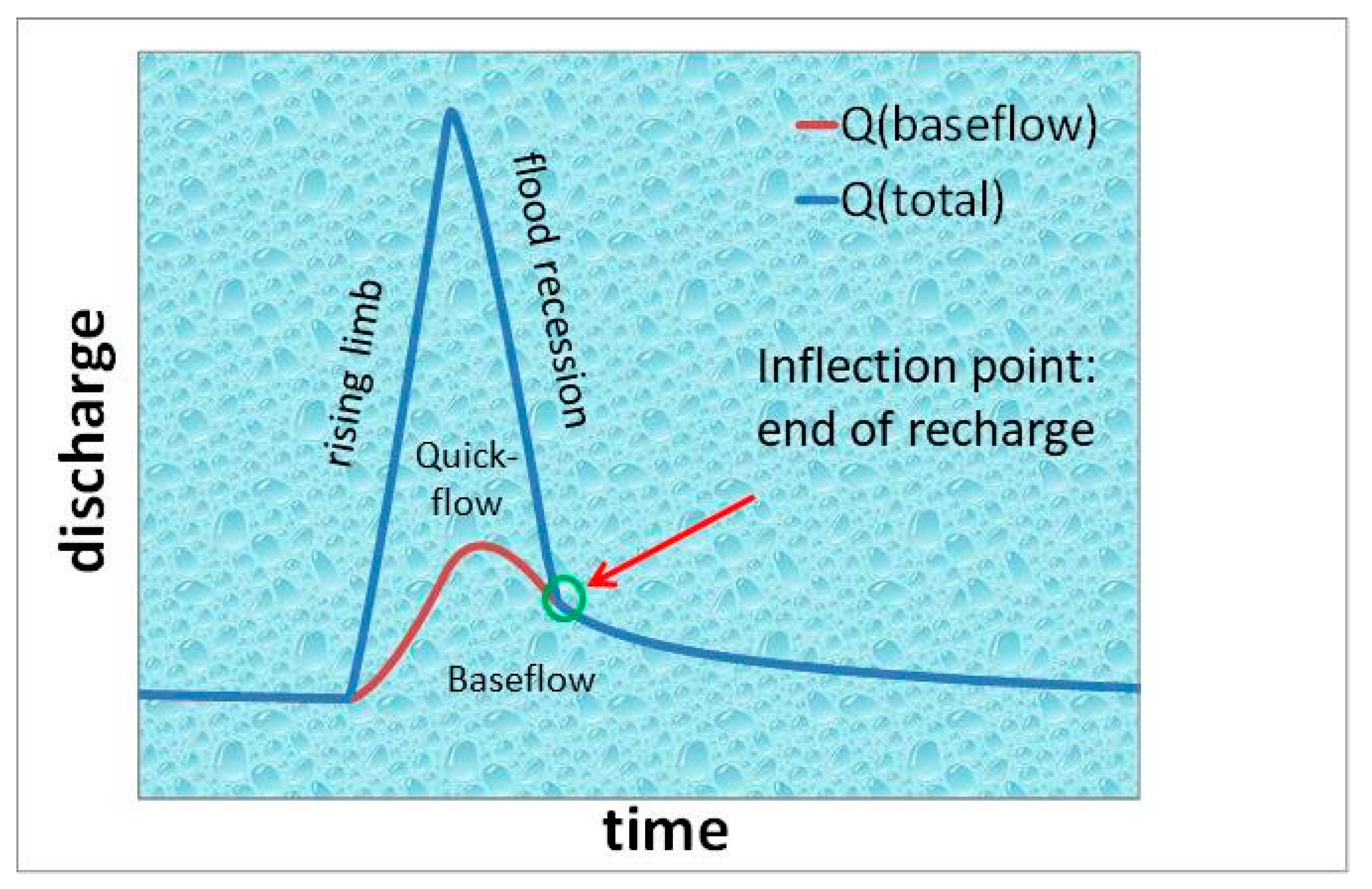
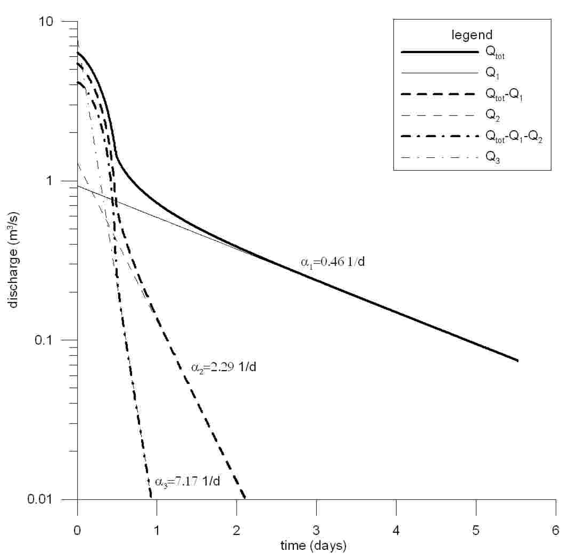
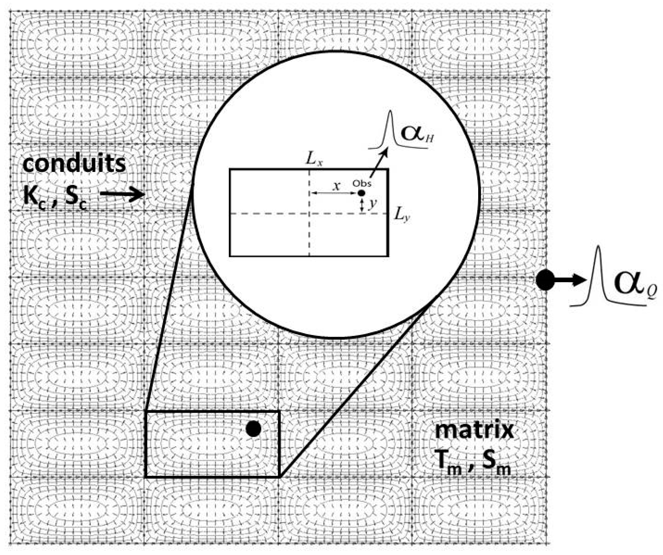
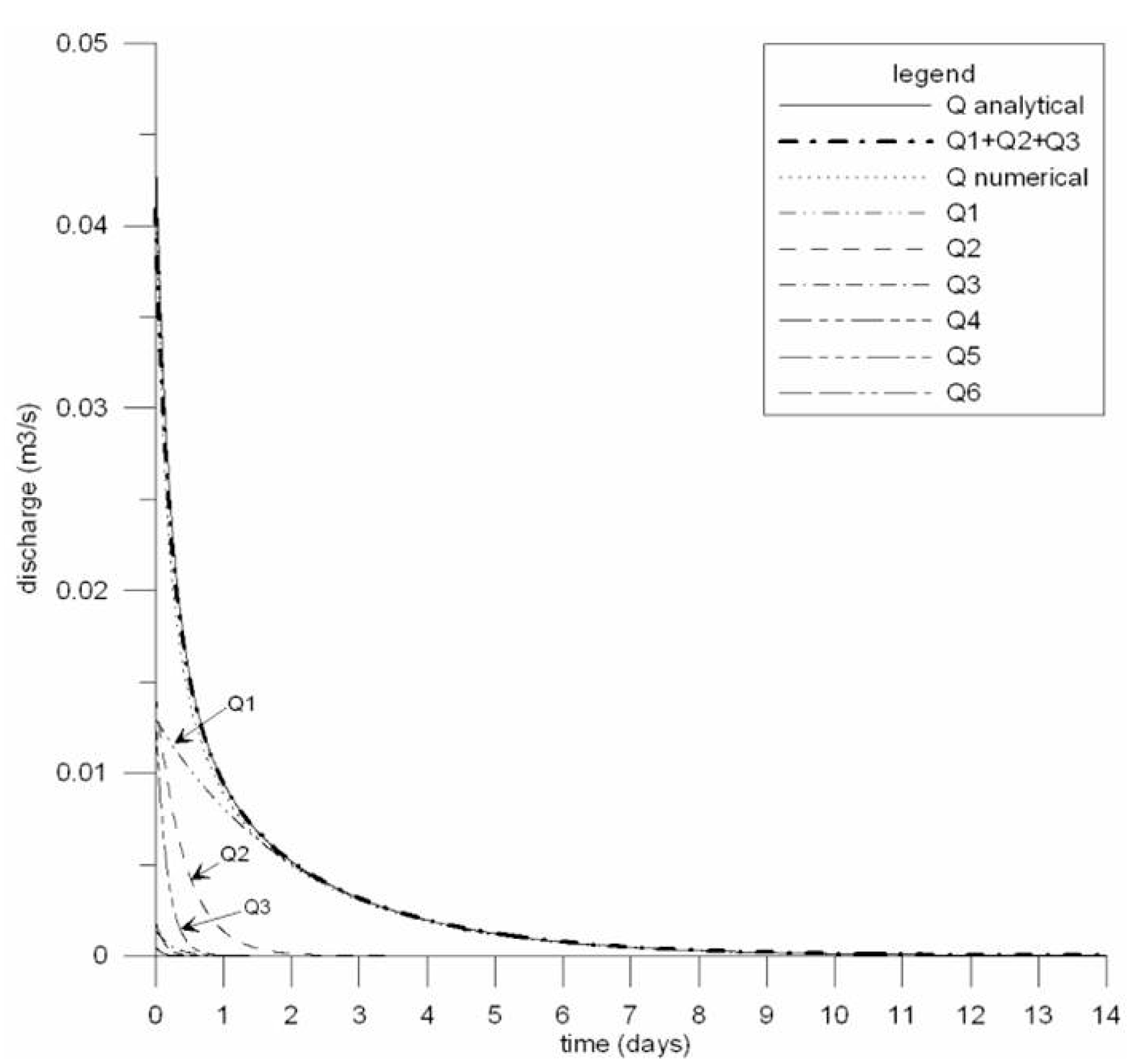
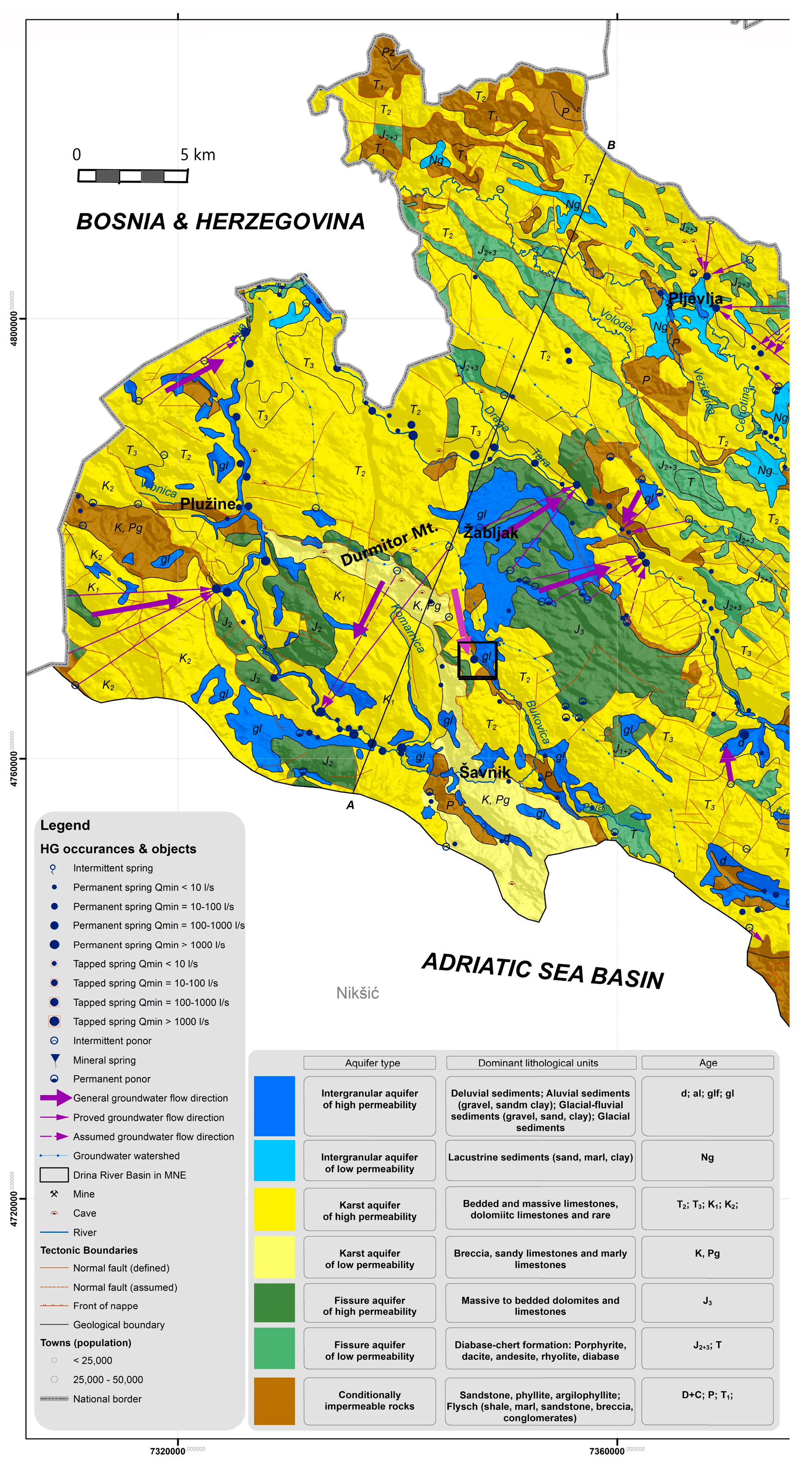
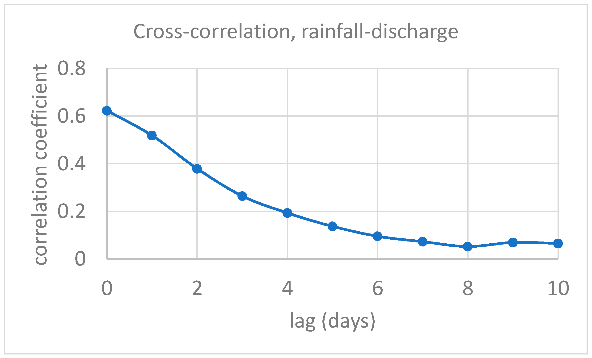
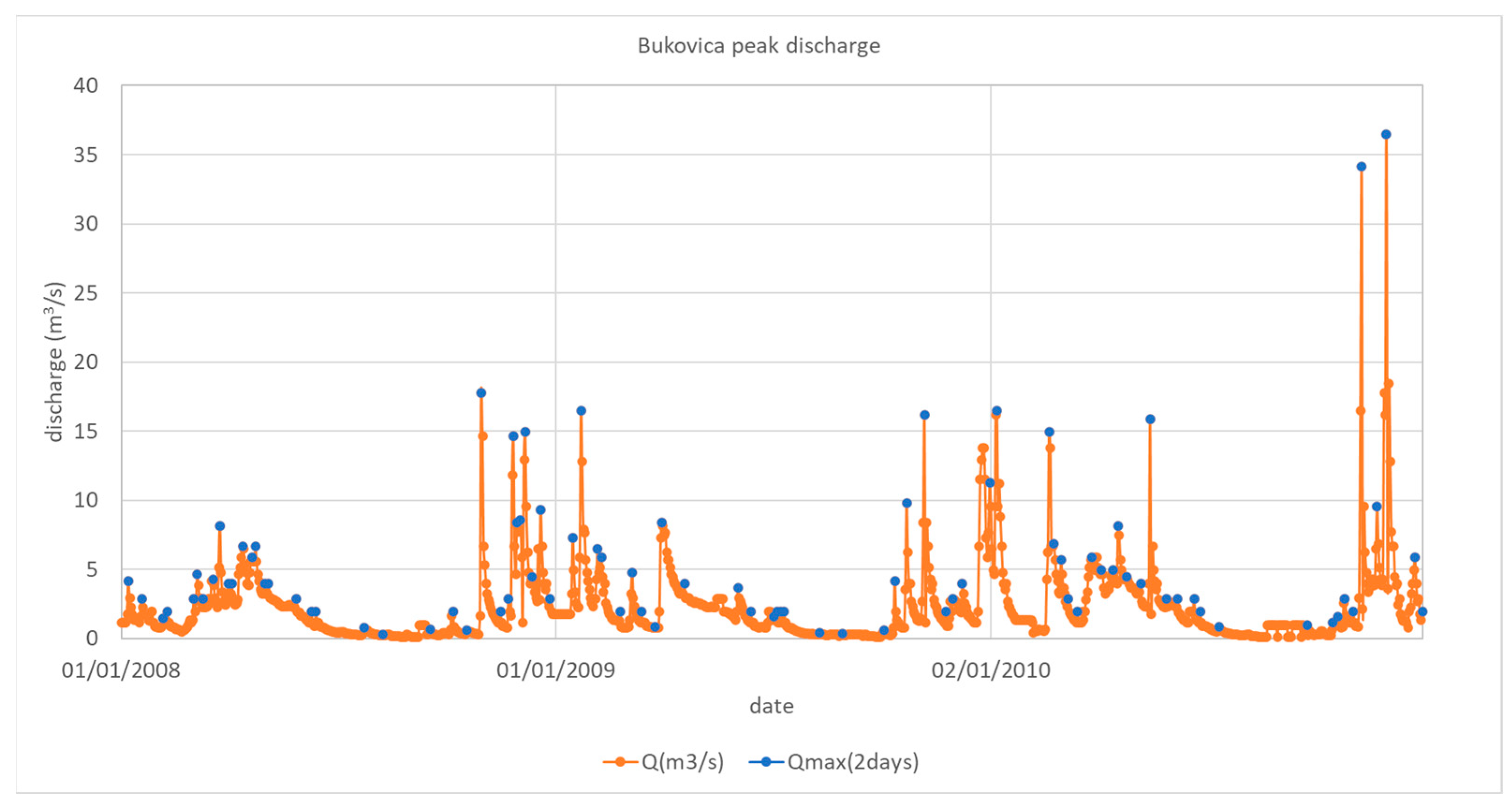
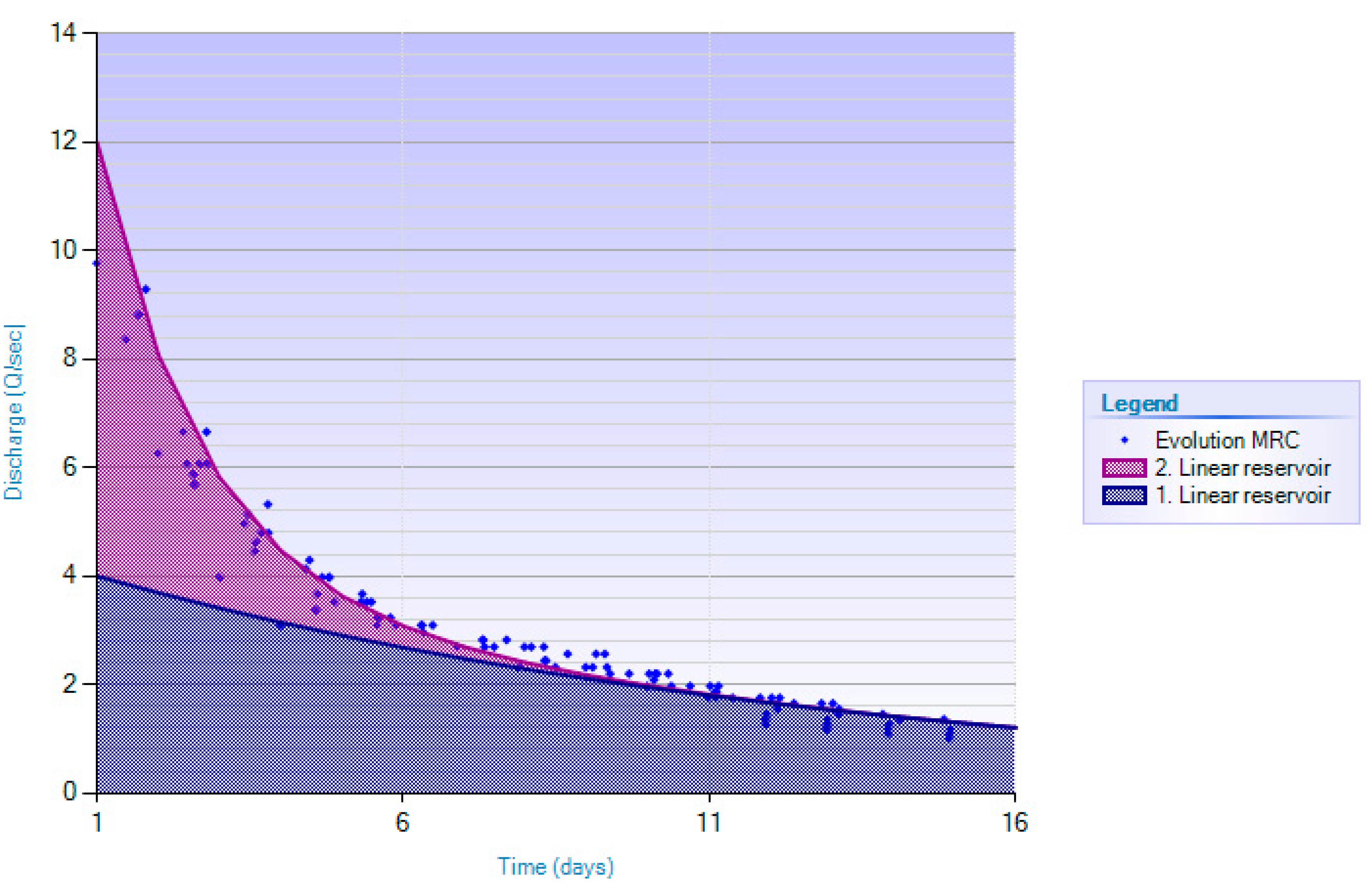
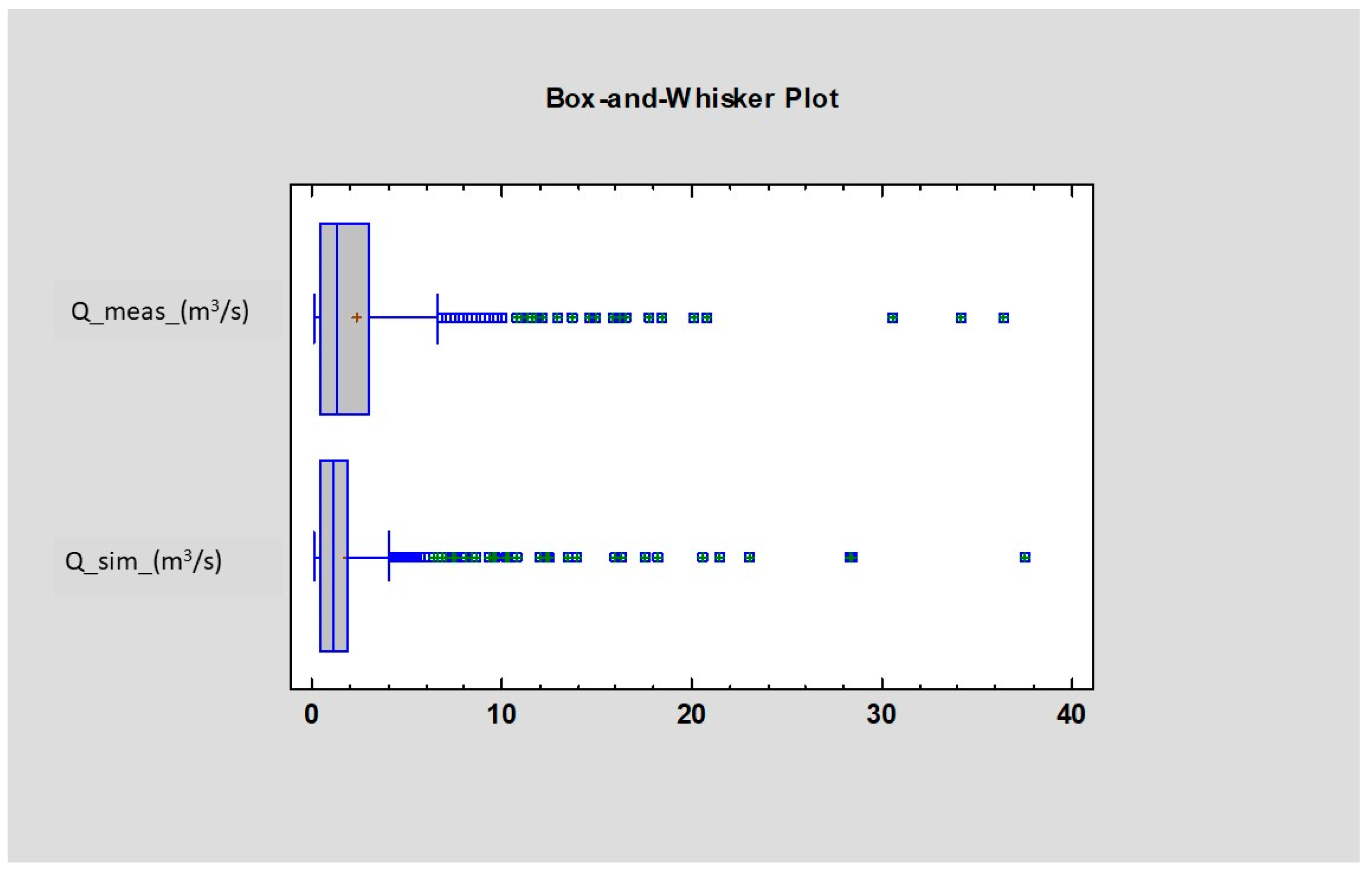
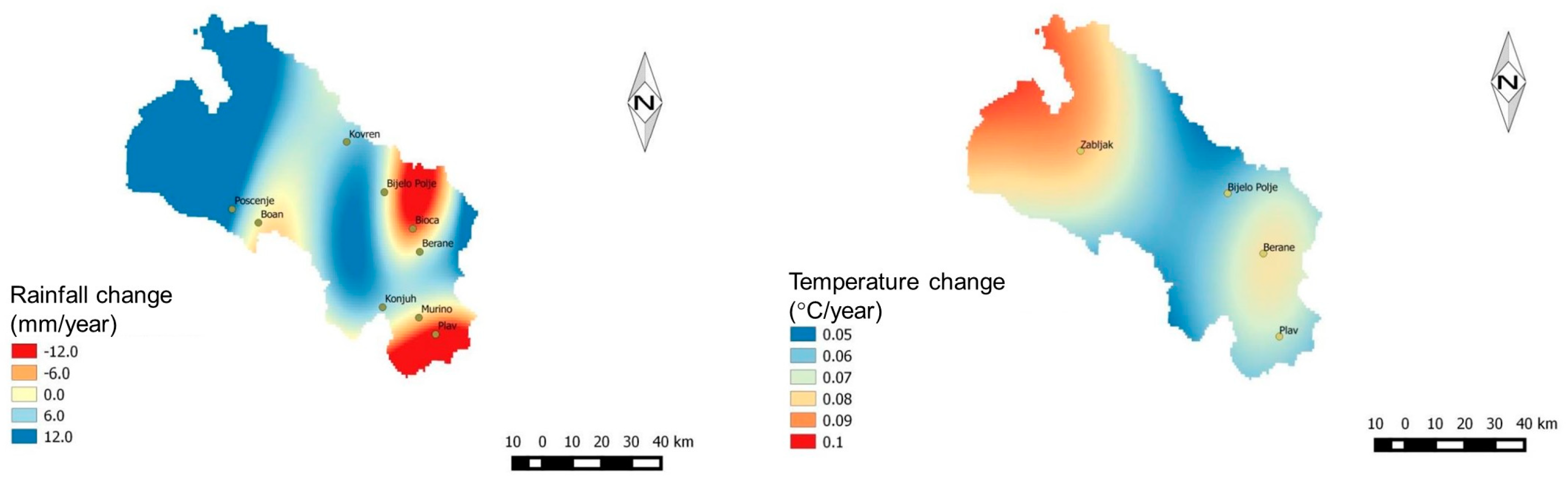
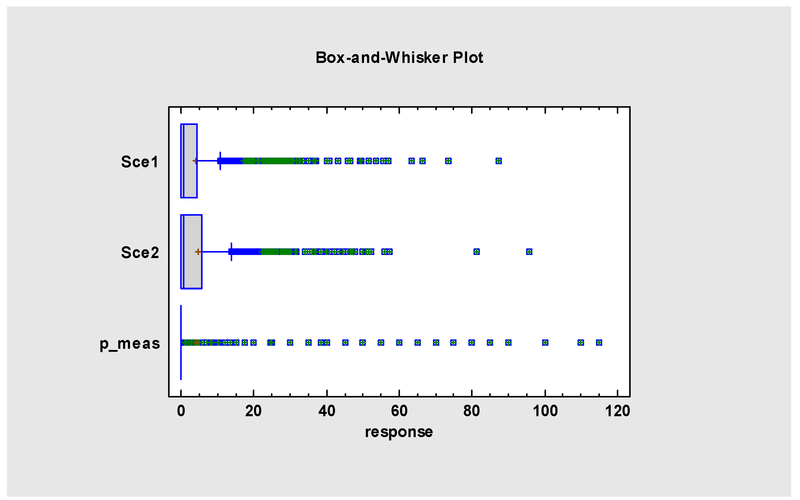
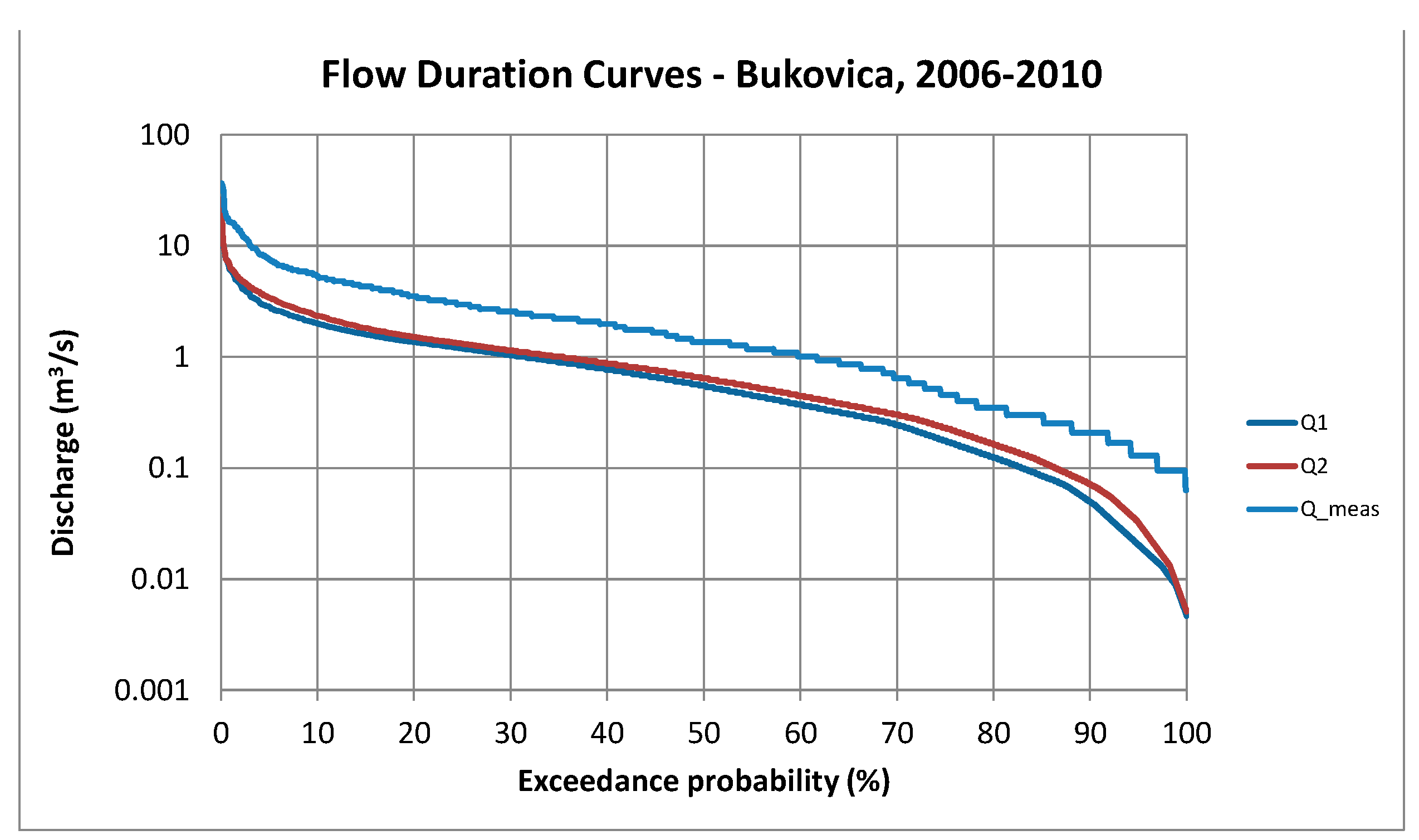
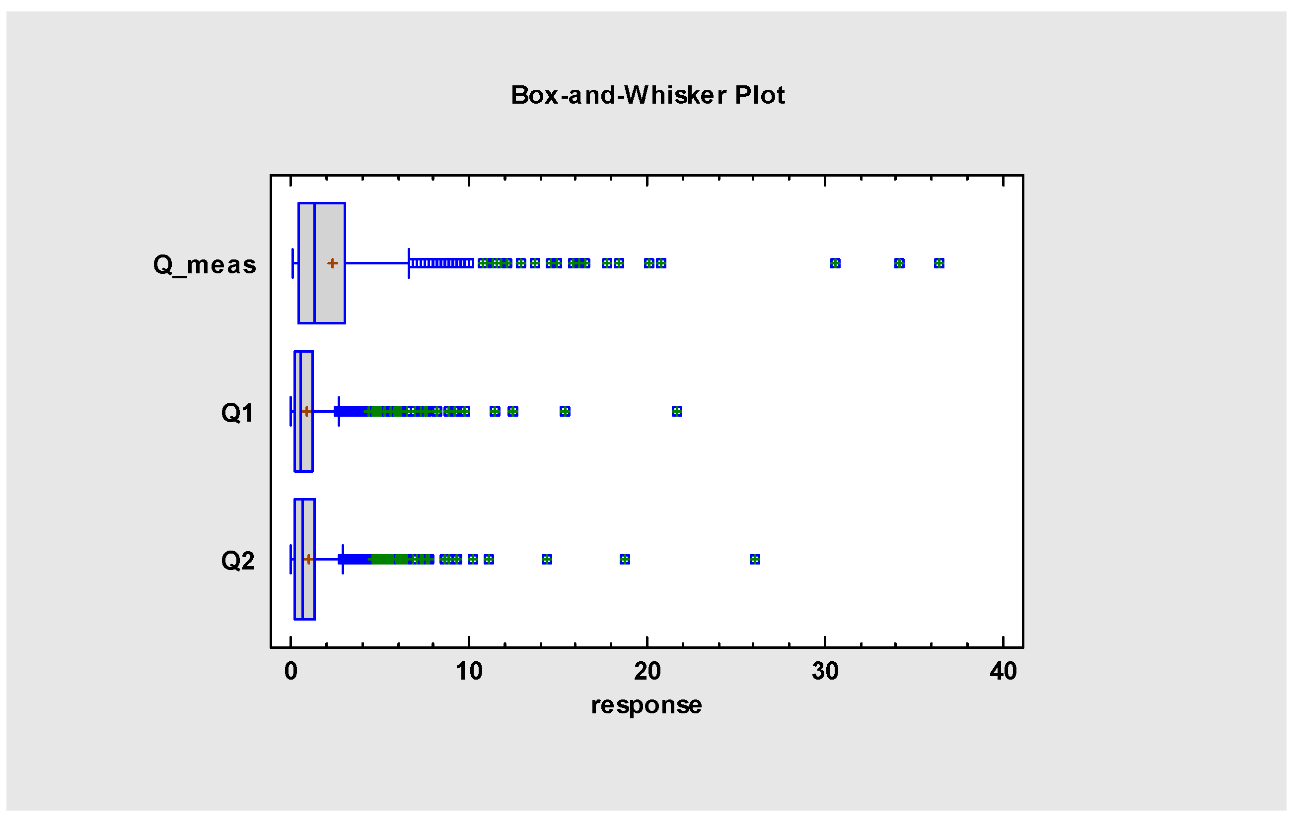
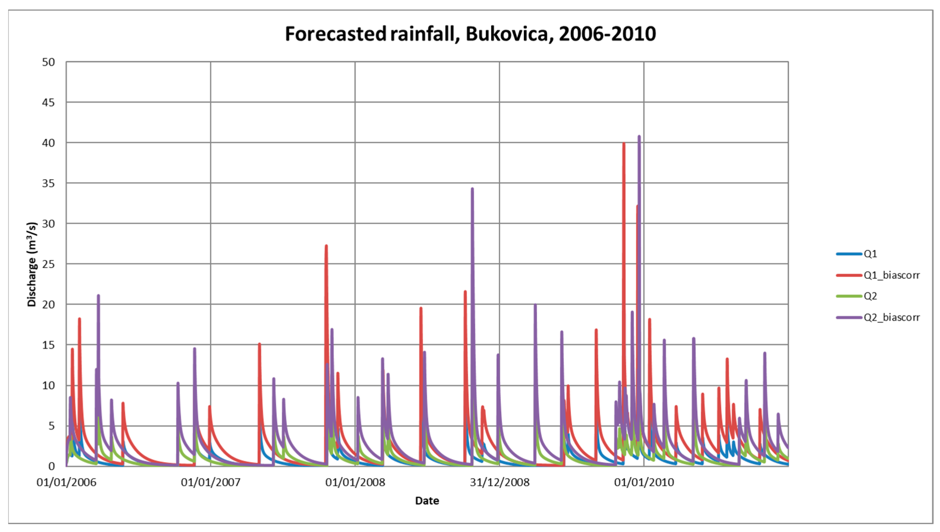
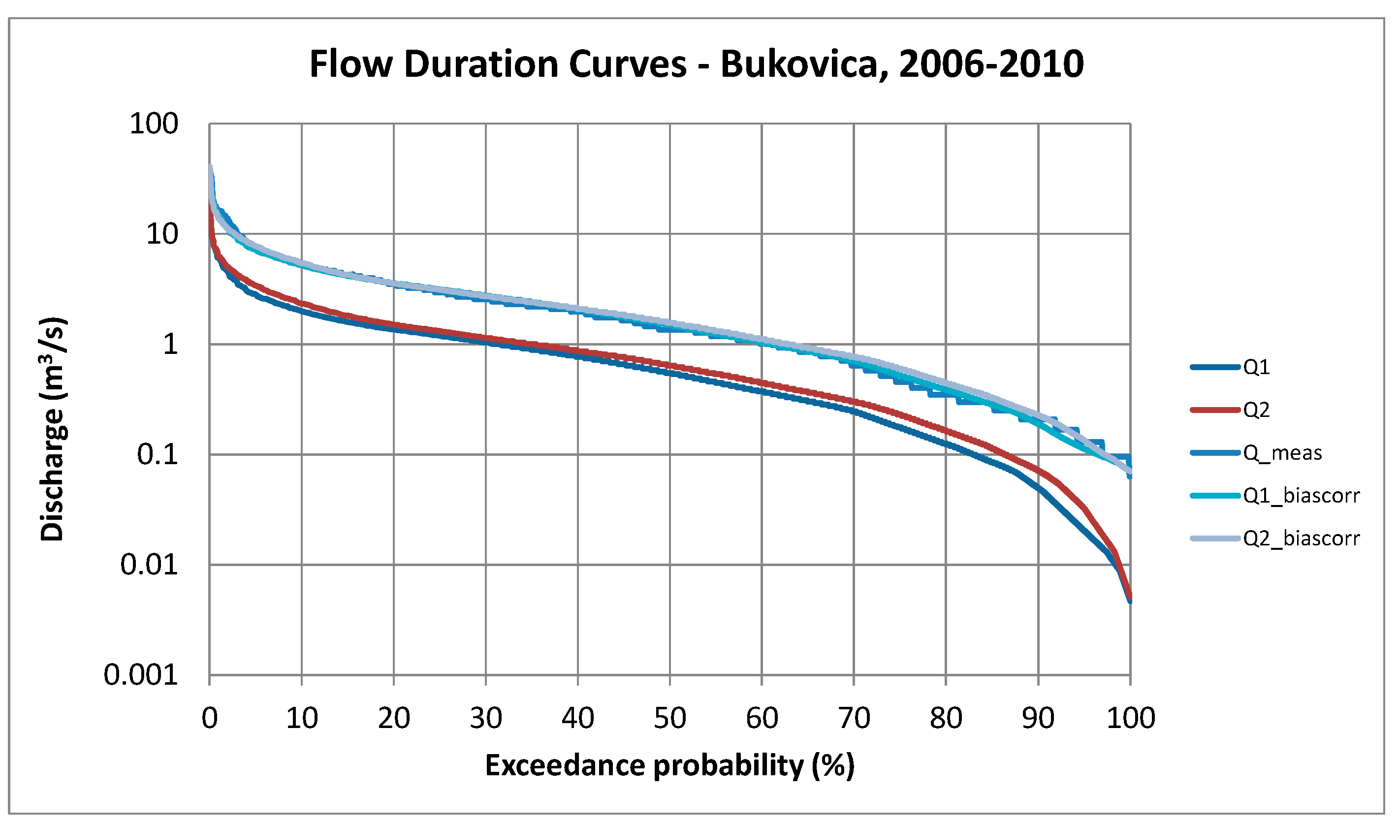
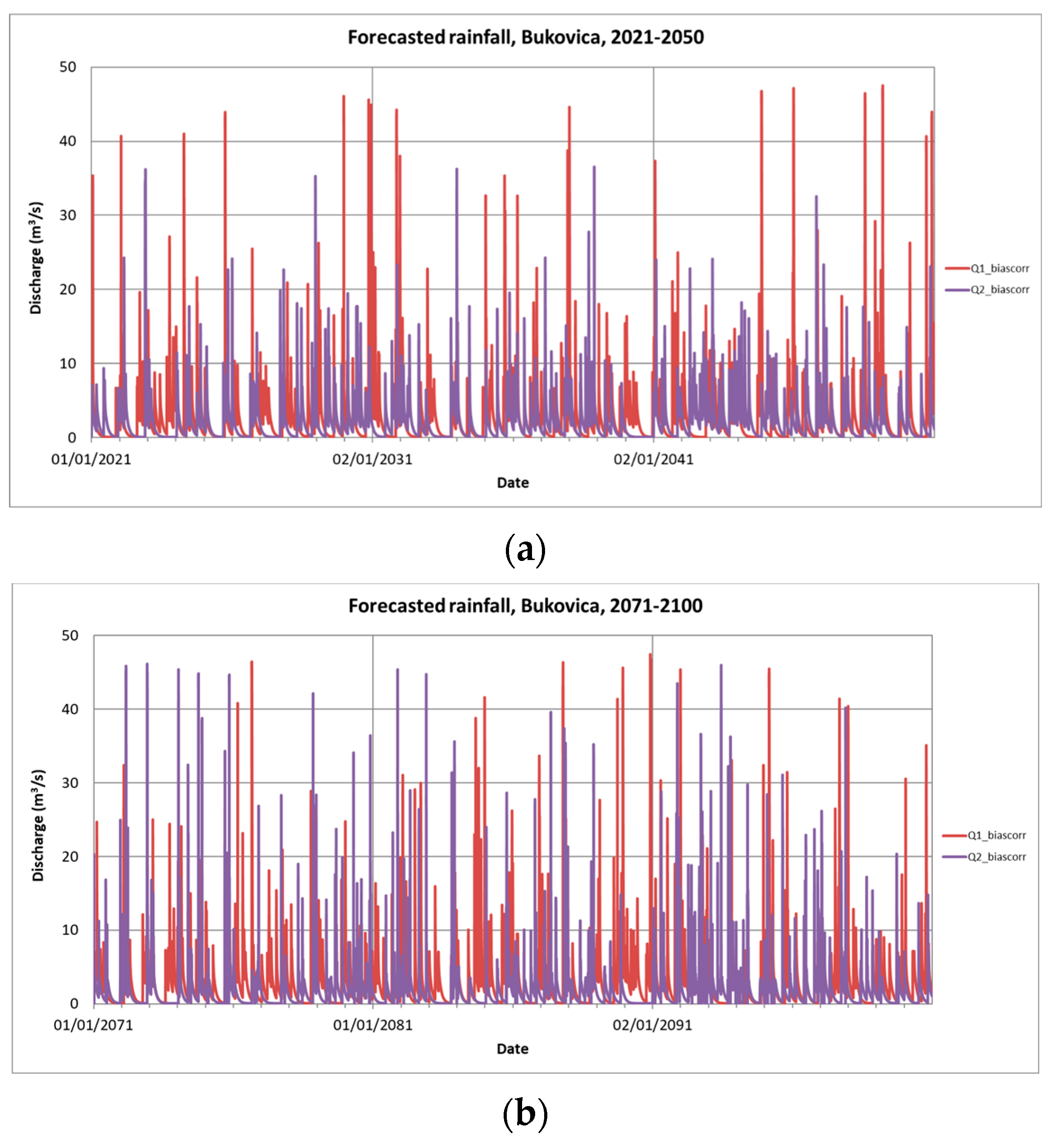
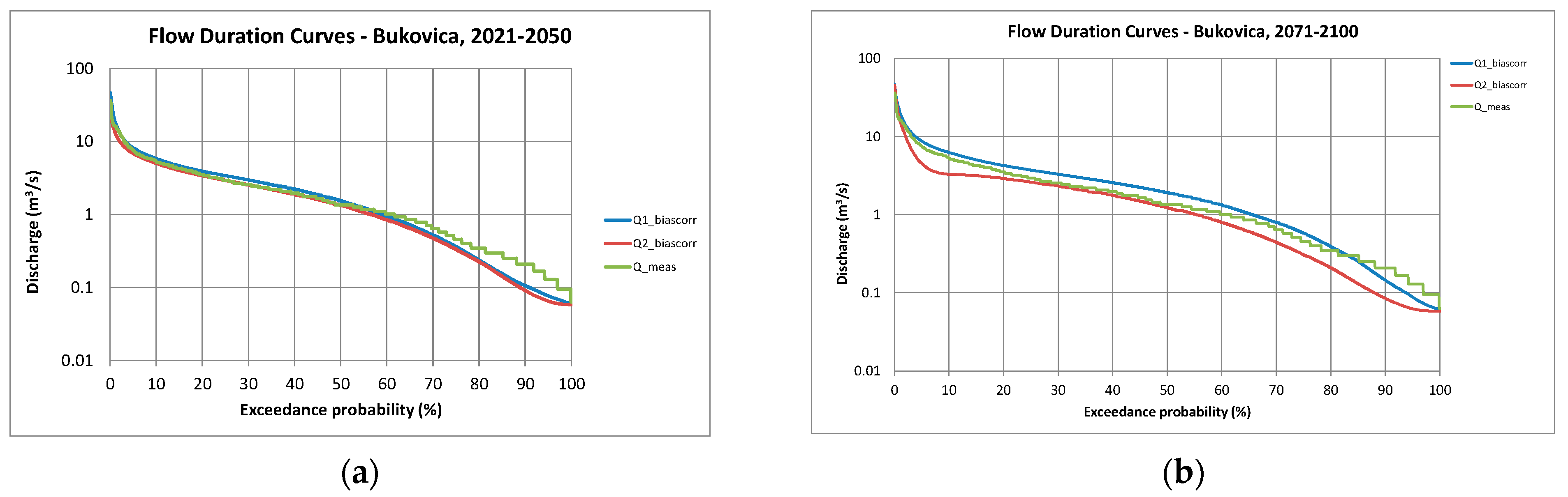
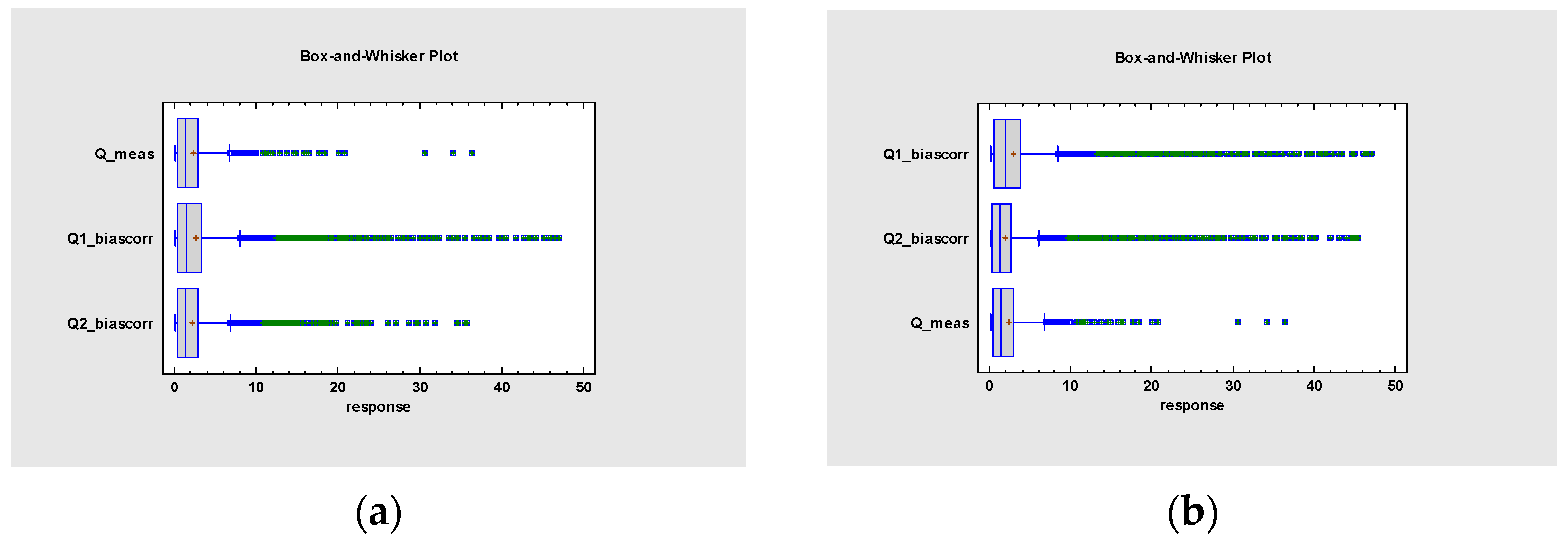
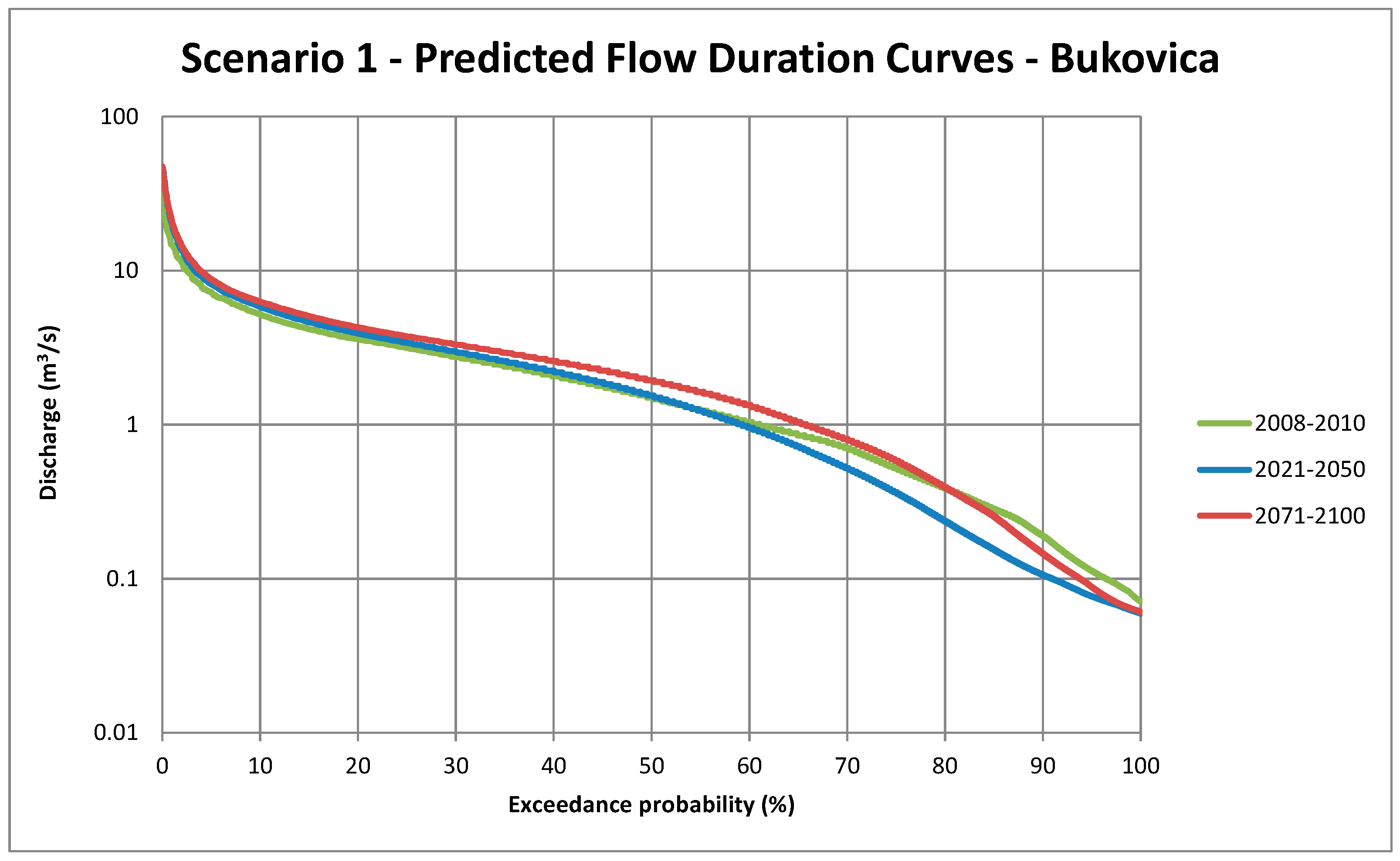
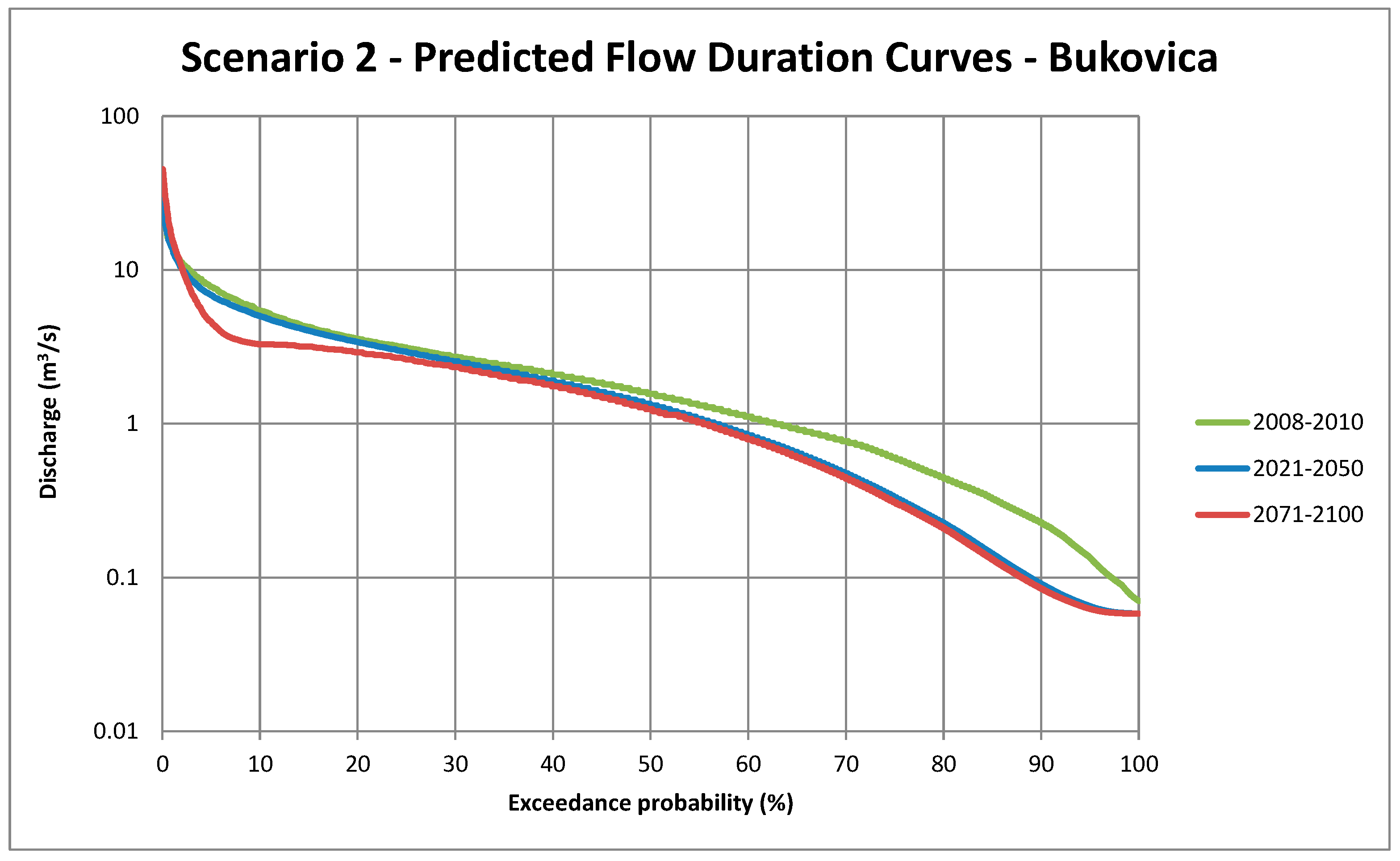
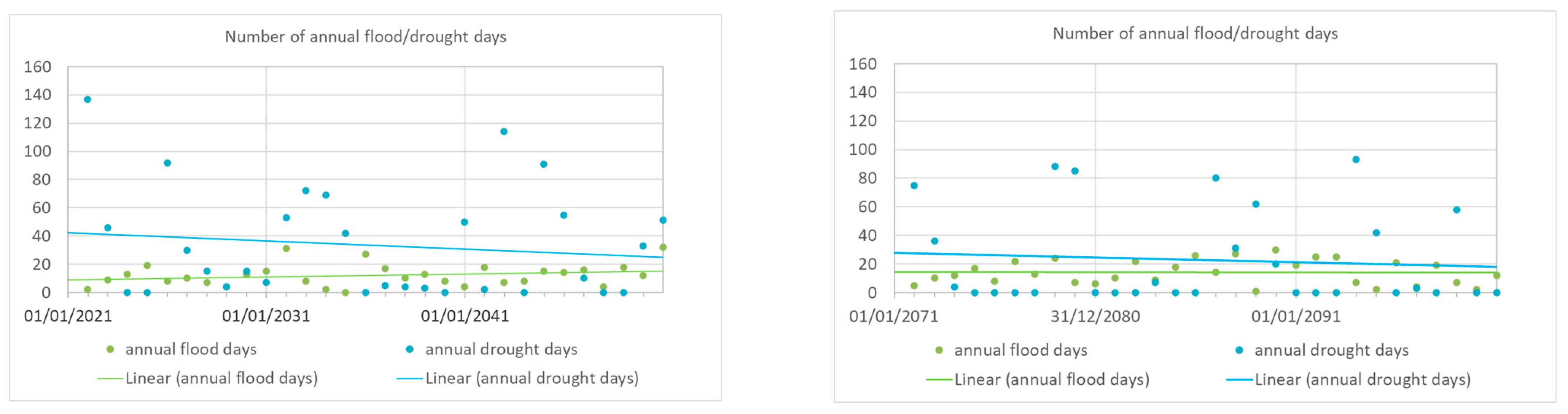
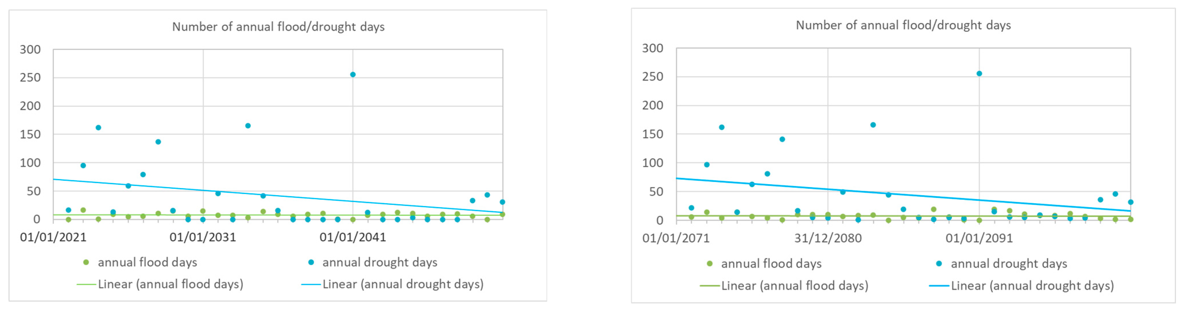
Table 1.
Investigated regional climate model projections.
| GCM | RCM | Scenario | Scenario Number |
|---|---|---|---|
| CNRM-CERFACS-CNRM-CM5 | CLMcom-CCLM4-8-17 | RCP45 | 1 |
| CNRM-CERFACS-CNRM-CM5 | CLMcom-CCLM4-8-17 | RCP85 | 2 |
Table 2.
Error statistics of regression analysis between rainfall and peak discharge.
| Statistical Measure | Value |
|---|---|
| Correlation coefficient | 0.82 |
| R-squared | 0.66 |
| Standard error of the estimate | 4.86 |
| Mean absolute error | 3.82 |
| Durbin–Watson statistic | 1.01 |
| Lag 1 residual autocorrelation | 0.49 |
| Correlation coefficient | 0.66 |
Table 3.
Summary statistics of applied models.
| Q_measured_(m3/s) | Q_simulated_(m3/s) | |
|---|---|---|
| Count | 1096 | 1095 |
| Average | 2.39 | 1.93 |
| Standard deviation | 3.27 | 3.11 |
| Variance | 10.72 | 9.65 |
| Coeff. Of variation | 137% | 161% |
| Minimum | 0.06 | 0.06 |
| Maximum | 36.45 | 37.60 |
| Range | 36.38 | 37.54 |
| Stnd. Skewness | 57.40 | 65.75 |
| Stnd. Kurtosis | 192.13 | 229.96 |
| Median | 1.36 | 1.05 |
Table 4.
Summary of statistics for regional rainfall projections.
| Count | Average | Standard Deviation | Coeff. of Variation | Minimum | Maximum | Range | Stnd. Skewness | |
|---|---|---|---|---|---|---|---|---|
| Scenario 1 | 1725 | 3.93 | 7.88 | 200% | 0 | 87.30 | 87.30 | 66.59 |
| Scenario 2 | 1725 | 4.56 | 8.51 | 187% | 0 | 95.80 | 95.80 | 59.77 |
| p_meas | 1725 | 4.24 | 11.91 | 281% | 0 | 115.00 | 115.00 | 74.12 |
Table 5.
Means with 95.0 percent LSD intervals, regional rainfall projections.
| Count | Mean | Stnd. Error | Lower Limit | Upper Limit | |
|---|---|---|---|---|---|
| Sce1 | 1725 | 3.93 | 0.23 | 3.61 | 4.25 |
| Sce2 | 1725 | 4.56 | 0.23 | 4.24 | 4.88 |
| p_meas | 1725 | 4.24 | 0.23 | 3.92 | 4.56 |
Table 6.
Summary statistics of multiple sample comparison amongst predicted and measured spring hydrographs.
Table 6.
Summary statistics of multiple sample comparison amongst predicted and measured spring hydrographs.
| Count | Average | Standard Deviation | Coeff. of Variation | Minimum | Maximum | Range | |
|---|---|---|---|---|---|---|---|
| Q_meas | 1096 | 2.39 | 3.27 | 137% | 0.06 | 36.45 | 36.38 |
| Q1 | 1825 | 0.90 | 1.28 | 141% | 0.0046 | 21.67 | 21.66 |
| Q2 | 1825 | 1.04 | 1.45 | 139% | 0.0051 | 26.09 | 26.09 |
Table 7.
Summary statistics of bias-corrected predicted and measured spring hydrographs for the 2021–2050 simulation period.
Table 7.
Summary statistics of bias-corrected predicted and measured spring hydrographs for the 2021–2050 simulation period.
| Q_meas. (m3/s) | Q1_biascorr. (m3/s) | Q2_biascorr. (m3/s) | |
|---|---|---|---|
| Count | 1096 | 10,957 | 10,957 |
| Average | 2.39 | 2.62 | 2.16 |
| Standard deviation | 3.27 | 3.96 | 2.83 |
| Coeff. of variation | 137% | 151% | 130% |
| Minimum | 0.063 | 0.059 | 0.058 |
| Maximum | 36.45 | 47.13 | 35.87 |
| Range | 36.38 | 47.07 | 35.81 |
| Stnd. skewness | 57.40 | 213.11 | 162.42 |
| Stnd. kurtosis | 192.13 | 799.15 | 533.03 |
Table 8.
Summary statistics of bias-corrected predicted and measured spring hydrographs for the 2071–2100 simulation period.
Table 8.
Summary statistics of bias-corrected predicted and measured spring hydrographs for the 2071–2100 simulation period.
| Q_meas. (m3/s) | Q1_biascorr. (m3/s) | Q2_biascorr. (m3/s) | |
|---|---|---|---|
| Count | 1096 | 10,957 | 10,957 |
| Average | 2.39 | 2.93 | 1.92 |
| Standard deviation | 3.27 | 4.02 | 3.24 |
| Coeff. of variation | 137% | 137% | 168% |
| Minimum | 0.06 | 0.06 | 0.06 |
| Maximum | 36.45 | 47.06 | 45.33 |
| Range | 36.38 | 47.00 | 45.27 |
| Stnd. skewness | 57.40 | 194.24 | 296.69 |
| Stnd. kurtosis | 192.13 | 672.02 | 1430.04 |
Table 9.
Summary statistics of Scenario 1’s bias-corrected predicted and measured spring hydrographs for the 2008–2010, 2021–2050, and 2071–2100 simulation periods.
Table 9.
Summary statistics of Scenario 1’s bias-corrected predicted and measured spring hydrographs for the 2008–2010, 2021–2050, and 2071–2100 simulation periods.
| Q1 | 2008–2010 | 2021–2050 | 2071–2100 |
|---|---|---|---|
| Count | 1825 | 10,957 | 10,957 |
| Average | 2.36 | 2.62 | 2.93 |
| Standard deviation | 2.97 | 3.96 | 4.02 |
| Coeff. of variation | 126% | 151% | 137% |
| Minimum (m3/s) | 0.07 | 0.06 | 0.06 |
| Maximum (m3/s) | 39.89 | 47.13 | 47.06 |
| Range (m3/s) | 39.82 | 47.07 | 47.00 |
| Stnd. skewness | 71.82 | 213.11 | 194.24 |
| Stnd. kurtosis | 260.29 | 799.15 | 672.02 |
Table 10.
Summary statistics of Scenario 2’s bias-corrected predicted spring hydrographs for the 2008–2010, 2021–2050, and 2071–2100 simulation periods.
Table 10.
Summary statistics of Scenario 2’s bias-corrected predicted spring hydrographs for the 2008–2010, 2021–2050, and 2071–2100 simulation periods.
| Q2 | 2008–2010 | 2021–2050 | 2071–2100 |
|---|---|---|---|
| Count | 1825 | 10,957 | 10,957 |
| Average | 2.42 | 2.16 | 1.92 |
| Standard deviation | 2.97 | 2.82 | 3.24 |
| Coeff. of variation | 122% | 130% | 168% |
| Minimum (m3/s) | 0.07 | 0.06 | 0.06 |
| Maximum (m3/s) | 40.79 | 35.87 | 45.33 |
| Range (m3/s) | 40.72 | 35.81 | 45.27 |
| Stnd. skewness | 69.80 | 162.42 | 296.69 |
| Stnd. kurtosis | 260.59 | 533.03 | 1430.04 |
Disclaimer/Publisher’s Note: The statements, opinions and data contained in all publications are solely those of the individual author(s) and contributor(s) and not of MDPI and/or the editor(s). MDPI and/or the editor(s) disclaim responsibility for any injury to people or property resulting from any ideas, methods, instructions or products referred to in the content. |
© 2023 by the authors. Licensee MDPI, Basel, Switzerland. This article is an open access article distributed under the terms and conditions of the Creative Commons Attribution (CC BY) license (https://creativecommons.org/licenses/by/4.0/).
Share and Cite
MDPI and ACS Style
Kovács, A.; Stevanović, Z. A Combined Stochastic–Analytical Method for the Assessment of Climate Change Impact on Spring Discharge. Water 2023, 15, 629. https://doi.org/10.3390/w15040629
AMA Style
Kovács A, Stevanović Z. A Combined Stochastic–Analytical Method for the Assessment of Climate Change Impact on Spring Discharge. Water. 2023; 15(4):629. https://doi.org/10.3390/w15040629
Chicago/Turabian StyleKovács, Attila, and Zoran Stevanović. 2023. "A Combined Stochastic–Analytical Method for the Assessment of Climate Change Impact on Spring Discharge" Water 15, no. 4: 629. https://doi.org/10.3390/w15040629
Note that from the first issue of 2016, this journal uses article numbers instead of page numbers. See further details here.