
Evolutionary Characteristics of Runoff in a Changing Environment: A Case Study of Dawen River, China
1
School of Water Conservancy and Hydropower, Xi’an University of Technology, Xi’an 710048, China
2
Post-Doctoral Research Center, Shandong Provincial Academician Workstation, Water Resources Research Institute of Shandong Province, Jinan 250014, China
3
State Laboratory of Water Resources and Hydropower Engineering Science, School of Water Resources and Hydropower Engineering, Wuhan University, Wuhan 430072, China
*
Author to whom correspondence should be addressed.
Water 2023, 15(4), 636; https://doi.org/10.3390/w15040636
Submission received: 26 November 2022
/
Revised: 12 January 2023
/
Accepted: 20 January 2023
/
Published: 6 February 2023
(This article belongs to the Special Issue Hydrological Responses under the Impacts of Climate Change and Human Activities)
Abstract
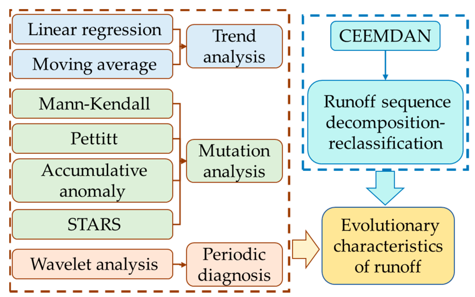
:Watershed water cycles undergo profound changes under changing environments. Analyses of runoff evolution characteristics are fundamental to our understanding of the evolution of water cycles under changing environments. In this study, linear regression, moving average, Mann–Kendall, Pettitt, accumulative anomaly, STARS, wavelet analysis, and CEEMDAN methods were used to analyze the trends, mutations, and periodic and intrinsic dynamic patterns of runoff evolution using long-term historical data. The intra-annual distribution of runoff in the Dawen River Basin was uneven, with an overall decreasing trend and mutations in 1975–1976. The main periods of runoff were 1.9 and 2.2 years, and the strongest oscillations in the study period occurred in 1978–1983. The runoff decomposition high-frequency term (intra-annual fluctuation term) had a stronger fluctuation frequency, with a period of 0.51–0.55 years, while the low-frequency term (interannual fluctuation term) had a period of 1.55–2.26 years. The trend term for the runoff decomposition tended to decrease throughout the monitoring period and gradually stabilized at the end of the monitoring period, while the period gradually decreased from upstream to downstream. In summary, we used multiple methods to analyze the evolutionary characteristics of runoff, which are of great relevance to the adaptive management of water resources under changing environments.
1. Introduction
The fourth report of the Intergovernmental Panel on Climate Change (IPCC) [1] stated that climate warming has led to significant changes in some features of the water and energy cycles. In addition to climate change, human activities such as irrigation farming, afforestation, deforestation, and urban construction have led to changes in hydrological processes, such as afforestation, reducing runoff [2] and urbanization and increasing surface runoff [3]. The United States Geological Survey (USGS) recently updated the water cycle diagram for the first time in 20 years [4]. In addition to natural processes, such as precipitation, evaporation, runoff, and lakes, the new water cycle schematic now includes human activities for the first time, such as industrial and agricultural water use, urban runoff, and reservoir behaviors, showing the role of humans in the overall water cycle process. Among the different components of the water cycle, runoff is the most important outcome of water resource management. The evolution of runoff significantly affects the patterns of water via different production sectors, such as the agriculture, domestic, industry, hydropower, and shipping sectors.
The impacts of environmental changes on watersheds are mainly reflected in the evolution of river runoff, which is increasingly influenced by human activities and climate change, mainly caused by global or regional human activities and increased climate change [5,6]. River runoff is the result of natural and anthropogenic influences and is one of the most important and easily exploitable forms of water resources [7]. As a key component of the hydrological cycle, the runoff has undergone substantial evolution with environmental changes [8,9]. Significant changes in runoff have been observed in 24% of the world’s rivers [10].
There is strong spatial and temporal heterogeneity in the variability of runoff from environmental changes. Since the beginning of the 20th century, the global average annual runoff has followed an increasing trend, while the average annual runoff has decreased in localized areas, such as the Pacific Northwest of the United States, the southeastern United States, and northern China [11]. Labat et al. studied the effects of global warming on runoff, and showed that an increase in global temperatures of 1 °C will increase global runoff by 4% [12]. Duan et al. (2017) studied the relative effects of climate variables on annual runoff in a region of the United States, and proposed that changes in runoff are mainly caused by precipitation [13]. In Canada, climate change typically leads to increases in mean annual runoff [14]. Surface runoff in the eastern part of southern Europe has tended to decrease, while that in the rest of the region has increased. From the Atlantic to the southern Gulf of Mexico region and the Pacific Northwest of the United States, river runoff is gradually decreasing. In the Yellow River Basin of China, there is an overall trend of decreasing surface runoff, with a 12% decrease in precipitation in summer and autumn [15]. However, in the Yangtze River Basin, the annual runoff has increased annually due to increased monsoon precipitation. One-third of the world’s top 200 rivers have experienced significant changes in runoff, either increasing or decreasing. With global warming and snow melt, the arrival date of maximum runoff in spring is occurring earlier, and snowfall events in winter are gradually turning into rainfall events, resulting in increased runoff in spring and winter, reduced runoff in summer, and the aggravation of drought. The forecast for global scale runoff shows that the average annual runoff will increase at high latitudes and in tropical humid regions, while that in most tropical dry regions will decrease. There is considerable uncertainty in the predicted results for regional runoff, both in terms of the quantity and trends.
Trend and mutation analyses are the main contents of runoff change research, and a large amount of research work has been carried out by domestic and foreign researchers for runoff change trends in different regions and watersheds [16,17,18,19]. The main methods of trend testing include parametric statistics such as linear regression analyses; accumulative anomaly and sliding t-tests; and non-parametric statistics such as the Mann–Kendall rank test, Spearman rank test, and Sen’s slope estimation. Since the methods are based on different principles, there are often differences between their calculation results, and the characteristics of the series such as autocorrelation and cyclical fluctuations may also lead to deviations in the analysis results when they are specifically applied [18]. Periodic diagnosis is another important element of runoff evolution characterization, and traditional analysis methods mainly use spectral analysis based on autocorrelation function or a Fourier transform [20], which has disadvantages such as its low resolution and serious frequency leakage, and is only applicable to stable and consistent time series [21,22]. The maximum entropy spectrum analysis (MESA) has the advantage of high resolution and adaptation to short sequences, and has become an important tool for hydrological sequence periodic identification [21,22]. A wavelet analysis can reveal the local characteristics of a sequence from the time and frequency domains, which is suitable for the study of sequences with multi-timescale variation and non-stationary characteristics, and is more widely used in the period identification and spatiotemporal scale variation analysis of runoff sequences [23,24,25]. With the introduction of theoretical approaches such as entropy, chaos, and fractals, the field of hydrological research has explored the non-linear and non-stationary nature of hydrological systems in greater depth. Huang et al. [26,27] proposed that the empirical mode decomposition (EMD) can be directly based on the sequence itself step by step decomposition, and described the different time scale oscillation characteristics and trend changes embedded in the series using a set of intrinsic mode functions (IMFs) characterizing the local changes of the original series, which provides better performance in describing the multi-scale change characteristics of non-stationary time series and has been more widely used.
Systematic analyses and identification studies of runoff evolution characteristics are fundamental in the research on water cycle evolution in basins under changing environments. They are important for analyzing the characteristics of runoff evolution using mathematical statistics and other techniques to evaluate the trends, periodicity, and spatial differentiation. To date, studies have investigated the characteristics of runoff evolution using a variety of research methods to elucidate these characteristics from different angles. However, there are limitations to the different methods used. A single method often cannot fully and effectively consider the complex characteristics of runoff evolution, and is limited by the length and quality of data in the study area. Thus, there remain limitations and uncertainties in our understanding of the characteristics of runoff evolution. Thus, the objectives of this study are: (1) to identify runoff evolution in the Dawen River Basin through trend, mutation, and periodic analyses of runoff series from 1961 to 2019; (2) by decomposing and reclassifying the runoff series itself, we describe the characteristics of oscillations and trend changes at different time scales embedded in the runoff series; (3) we integrate multiple methods to improve the credibility of runoff evolution characteristics, and provide scientific support for managers to develop and manage regional water resources and cope with the changing environment.
2. Materials and Methods
2.1. Study Area
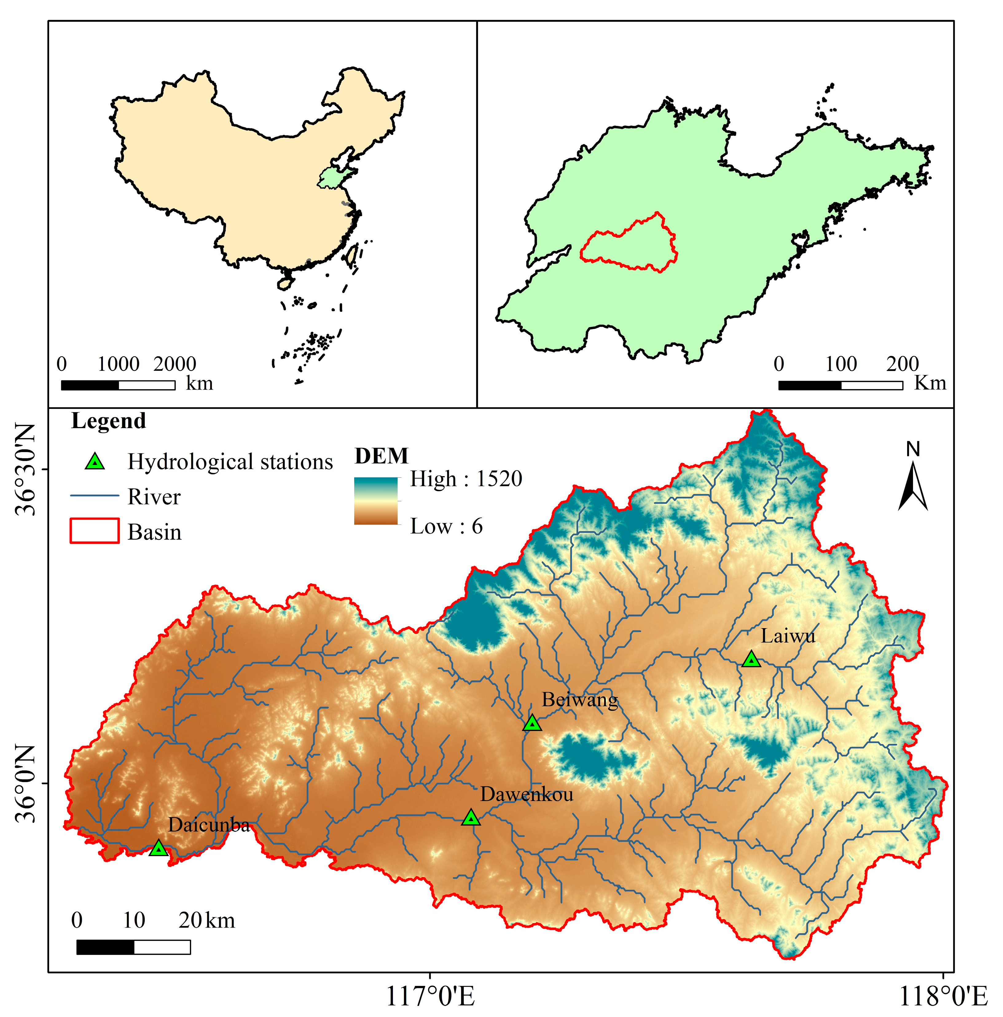
The Dawen River is the largest tributary of the lower reaches of the Yellow River in Shandong Province, and is one of the few rivers in China that flows from east to west. The Dawen River originates in Laiwu City, flows through Tai’an City, and merges into Dongping Lake from east to west (Dongping Lake is the only important flood storage and detention area in the Yellow River basin, and the source of the national South-to-North Water Transfer East Line storage hub and Shandong Jiaodong Water Transfer Project), and then enters the main channel of the Yellow River through Qinghe Lock. It has a total length of 231 km and a watershed area of 8944 km2. The natural water resources in the Dawen River Basin are more abundant than in the whole region of Shandong; however, due to frequent human activities, the construction of a large amount of water infrastructure on the river, coupled with the impact of climate change, the river has undergone periodic disruption. The river runoff deviates significantly from its natural evolution; if we do not fully understand the basin hydrology, particularly the variation in river runoff, the water security risk may be very high. The ecological protection and high-quality development of the Yellow River basin is a major national strategy [16]. The Dawen River Basin is the main battlefield for ecological protection and the high-quality development of the lower reaches of the Yellow River, and an important position for ensuring the safety of the Yellow River and the water quality of the South-to-North Water Diversion Project (Figure 1).
2.2. Data
The monthly runoff data used in this study were obtained between 1961 and 2019 from the hydrological stations of Laiwu, Beiwang, Dawenkou, and Daicunba, which were sourced from the Shandong Provincial Hydrological Bureau.
2.3. Methods
2.3.1. Trend Analysis
A series of climate data that change over time constitutes a climate time series. These variables are usually random series obtained by discrete observations, with the following characteristics: the data values vary with time; the randomness of the values at each moment; the correlation and continuity between data before and after the moment; the sequence as a whole has an upward or downward trend and shows periodic oscillations; there is a turn or abrupt change at a certain moment. A trend analysis involves the analysis of continuous increases or decreases in the time series of hydrometeorological elements over a long time period. In this study, linear tendency estimates and moving averages were used to analyze the trend characteristics of the time series.
- (1)
- Linear tendency estimation
A climate variable with sample size n (sample size n ≥ 30) is represented by , and the time corresponding to is represented by . A unitary linear regression is established between and , as follows:
Equation (1) is a simple linear regression, and is a typical method used for time series analyses. Where is the regression constant and is the regression coefficient, and can be estimated using the least squares method as follows:
The correlation coefficient between the time and variables is calculated as follows:
The linear regression results are expressed by analyzing the regression coefficient and the correlation coefficient . The symbol of the regression coefficient indicates the trend tendency of the climate variable . When , increases with time ; when , decreases with time . The magnitude of reflects the rate of increase or decrease, i.e., it indicates the degree of the tendency to increase or decrease. Therefore, is usually referred to as the tendency value; this method is termed a linear tendency estimation.
The correlation coefficient indicates the closeness of the linear correlation between the variable and time . The closer is to 0, the smaller the linear correlation between and . Conversely, the closer is to 1, the closer the linear correlation between and . It is also necessary to determine whether the degree of the trend change is significant and to determine the significance level α. If , this indicates that the change in the trend of with time is significant, otherwise it is not significant.
- (2)
- Moving average
The moving average is a basic method to test for trendiness. It is similar to the low-pass filter. For the sequence with a sample size of , its moving average sequence is expressed as:
where is the moving length; is generally taken as an odd number so that the average can be added to the time coordinate of the time series term. After a moving average, the period in the series about the moving length is greatly weakened, showing a trend of change. The moving average series graph is viewed to diagnose the trend of change.
2.3.2. Mutation Analysis
Mutation is the phenomenon of discontinuous change in climate variables, jumping from one stable state to another, meaning is a quantitative change to a certain degree will become a qualitative change. Mutation is the node of the mutation point, and the change trends before and after the sequence are inconsistent. The “jump” at a certain point (the jump point is removed and the stable states before and after are consistent) is not a mutation. There are many controversies in the application of mutation theory, and different test methods may yield multiple mutation results. In practice, multiple methods should be compared and combined with professional knowledge to analyze the rationality of mutation phenomena, in order to make a scientific judgment. In this study, Mann–Kendall, Pettitt, accumulative anomaly, and regime shift detection techniques were used to identify mutation points.
- (1)
- Mann–Kendall Method
The principle of the Mann–Kendall (M-K) method was originally proposed and developed by Mann and Kendall [28,29]. Subsequently, it has been improved and refined, is recommended by the World Meteorological Organization, and is widely used in the field of meteorology. The Mann–Kendall method is a rank-based non-parametric statistical test, which does not require the assumed distribution of random variables, meaning it is a distribution-free test. The abnormal values in the sample sequence will not significantly affect the sample test results; thus, it is more suitable for testing the type and sequential variables [30].
- (2)
- Pettitt Method
The Pettitt method is a non-parametric test method, which was first applied by Pettitt to test mutation points [31]. This test is used to evaluate the possible location of a single mutation point. It is an order-based and distribution-free method, which is used when the exact time of the mutation is unknown, similar to the Mann–Kendall method.
- (3)
- Accumulative Anomaly Method
The accumulative anomaly is used to evaluation mutation based on the trend of the curve. The accumulative anomaly of sequence at time t is expressed as follows:
The accumulative anomaly curve is plotted with the calculated accumulative anomaly values at moments at a time to analyze the trendiness, observe the trend of the accumulative anomaly curve, determine the long-term evolutionary trend and changes, and elucidate the approximate time of mutation occurrence.
- (4)
- Regime Shift Detection (STARS) Method
The regime shift detection method [32,33], also known as STARS (the sequential-test analysis of regime shifts), is a non-parametric method of mutation detection. It is used to explain the “state” and “state transition” of long-term climate change, which is defined as the rapid transition of climate ecosystems from one relatively stable state to another. This concept was strongly promoted in the late 1970s when the global climate system underwent a step change, identifying the state transition points, or mutation points, by seeking the mean and variance shifts. This method can detect the moment and magnitude of the state transition, and can quantitatively and visually obtain the pattern transition point [34].
2.3.3. Periodic Diagnosis
In recent years, the wavelet analysis method has been used to perform periodic diagnoses. The wavelet analysis method is a breakthrough in Fourier analysis methods [35]. The wavelet transform has a solid mathematical foundation, and can determine the scale of time series changes and the locations at which they occur.
The results obtained via wavelet transform can be analyzed as follows: using the adjustable resolution, the fine part can be enlarged, enabling the local structure and characteristics to be analyzed; local singularities located at the wavelet coefficient oscillation can be evaluated, and the time positions of different scales can be determined to distinguish the sudden change signal, to analyze the sequence in stages, and to make climate predictions according to the above analysis. The figure shows the evolution of different cycles over time and can be used to determine the significant cycles. Wavelet variance can determine which length cycle has the strongest vibration, and can also confirm which cycle length has the strongest vibration in which time period based on the segmented wavelet variance.
2.3.4. Runoff Sequence Decomposition–Reclassification Method
In this study, CEEMDAN (complete ensemble empirical mode decomposition with adaptive noise) was used to decompose the runoff sequence when analyzing the characteristics of long-term monthly runoff series. Thus, the decomposed data were reclassified into high-frequency terms, low-frequency terms, and trend terms based on the percentages of variance classes to analyze the intra-annual fluctuation characteristics, interannual fluctuation characteristics, and long-term runoff trends. The CEEMDAN method is suitable for analyzing the decomposition of adaptive non-stationary and non-linear data, and its main principle is to decompose the original data into intrinsic mode functions (IMF) of different frequency series based on its decomposition principle. The CEEMDAN method is mainly based on the EMD (empirical-mode decomposition) and EEMD (ensemble empirical-mode decomposition) methods. The main improvement is the addition of adaptive white noise to the EMD method to reduce modal aliasing. The main principle of the method is as follows [26,36,37,38]:
Stage (1) defines a long series of raw data, which is set as the original input signal:
where ωi(t) is the white noise sequence and ε is the noise coefficient.
Stage (2) decomposes IMF1. The first IMF and average IMF are calculated using the EMD method:
Its residuals are then refined:
Stage (3) decomposes IMF2:
Stage (4) decomposes the other IMFs until the limit value is less than 2. The final signal sequence is decomposed as follows:
CEEMDAN can decompose the original data into different IMF sequences and extract their different frequency features from the IMF sequences, using high frequency, low frequency, and trend terms. In this study, the IMF sequences were reclassified using the variance occupation ratio.
Based on the above, multiple methods were integrated to analyze the runoff evolution characteristics. The procedure of the integrated framework is shown in Figure 2.
3. Results and Discussion
In this study, the spatial and temporal evolution characteristics of the runoff were analyzed at the hydrological stations of Laiwu, Beiwang, Dawenkou, and Daicunba from the upstream to downstream of the Dawen River.
3.1. Trend Analysis
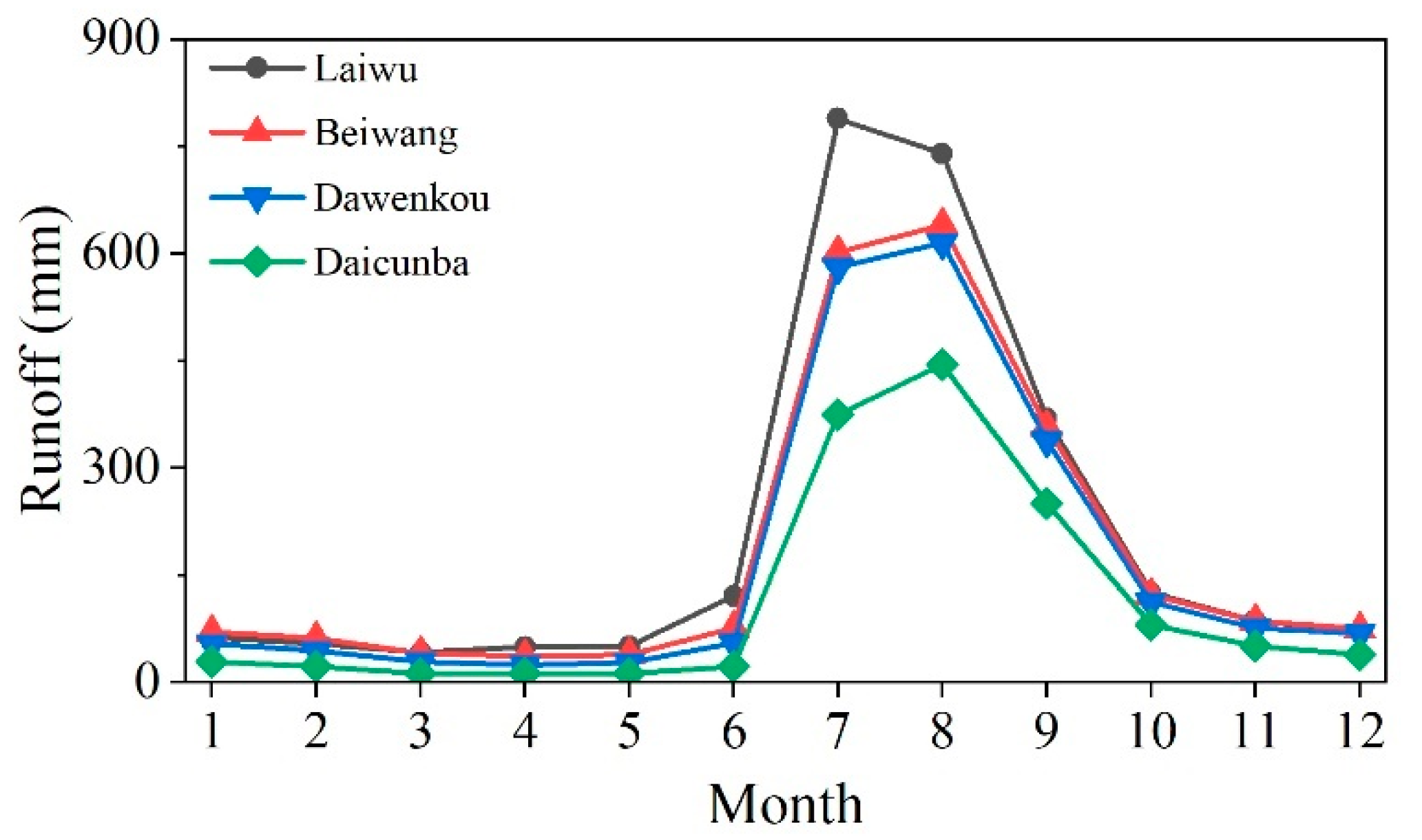
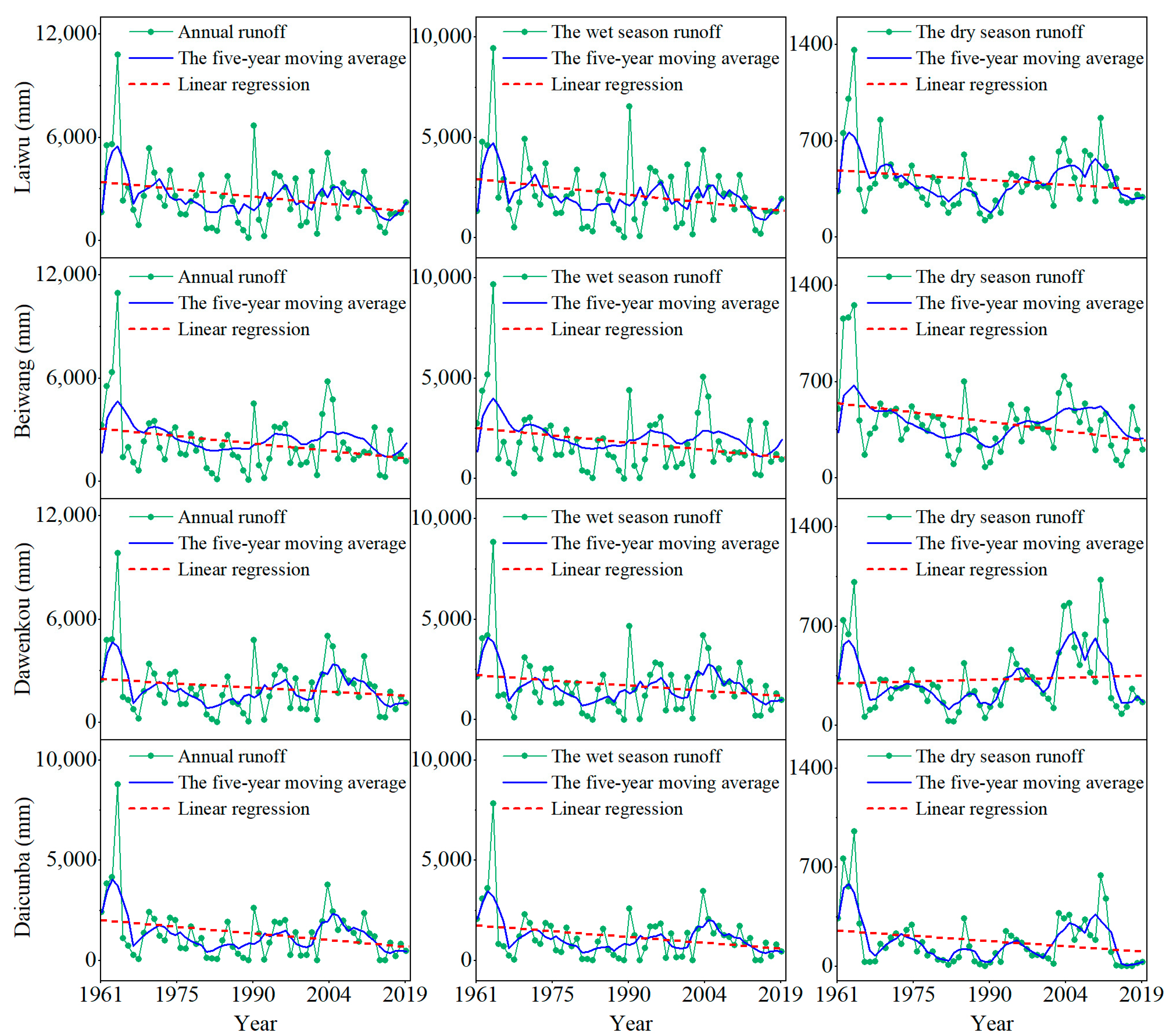
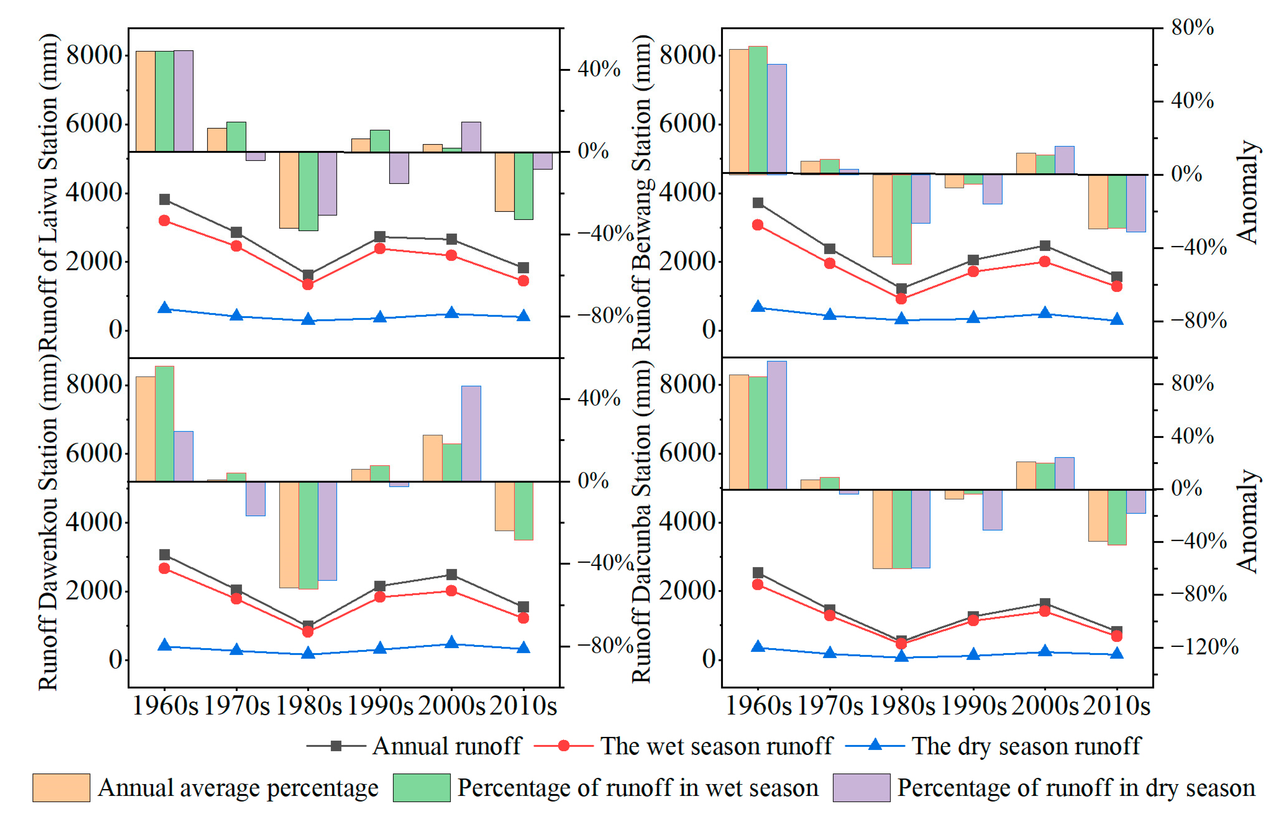
As shown in Figure 3, the intra-annual distribution of runoff in the Dawen River Basin is extremely uneven, with the runoff decreasing sequentially from upstream to downstream at Laiwu, Beiwang, Dawenkou, and Daicunba. The runoff from the four hydrological stations is mainly concentrated in June to October during the abundant water period, accounting for 84–87% of the annual runoff, while that during the dry period (November–May) is less abundant, accounting for 13–18% of the annual runoff. The annual runoff, abundant water season runoff, and drought water season runoff were analyzed for each hydrological station in the Dawen River Basin from 1961 to 2019. As shown in Figure 4 and Table 1, with the exception the Dawenkou hydrological station, which showed an increasing trend in runoff during the dry period (which did not pass the significance test), the other stations presented decreasing trends in runoff on different time scales. Among the four hydrological stations, the runoff at the Dawenkou and Laiwu stations during the dry period presented insignificant trends, while the other runoffs presented significant trend changes. This indicated that the runoff of Dawen River Basin shows a significant decreasing trend. According to the five-year moving average variation curves, the dynamics of annual runoff and runoff during the abundant water period from 1961 to 2019 are consistent in pace with time, while the dynamics of change during the dry water period differ. This, further illustrates the uneven intra-annual distribution of runoff in the Dawen River Basin, with the runoff during the abundant water period providing the greatest contribution to the annual runoff.
The interdecadal variation in runoff at the Dawen River Basin was analyzed, as shown in Table 2 and Figure 5. The runoff at all hydrological stations in the Dawen River Basin was highest in 1961–1969, with varying increases in runoff compared to the multi-year average (1961–2019), especially at Beiwang and Daicunba stations, which accounted for 60–98% of the multi-year average runoff. The runoff was lower in the 1980s and 2010s. In the 1980s, the runoff rates were reduced by 30–39, 26–49, 48–53, and 59–61% compared with the multi-year average runoff at Laiwu, Beiwang, Dawenkou, and Daicunba stations, respectively. In the 2010s, the runoff rates were reduced by 8–33, 29–32, 0–29, and 18–40%, respectively, compared with the multi-year average runoff at Laiwu, Beiwang, Dawenkou, and Daicunba stations. Thus, the runoff decreases continuously from upstream to downstream, and the variation dynamics and amplitude of the interannual runoff are consistent in the abundant water season, with differences in the fluctuation state of runoff in the dry season. This is likely to be caused by the more frequent water extraction activities in the middle and lower reaches.
The runoff variation of the Dawen River Basin was similar to that of the Yellow River Basin, with an attenuation tendency, while the annual distribution was uneven and the interdecadal variation differed.
3.2. Mutation Analysis
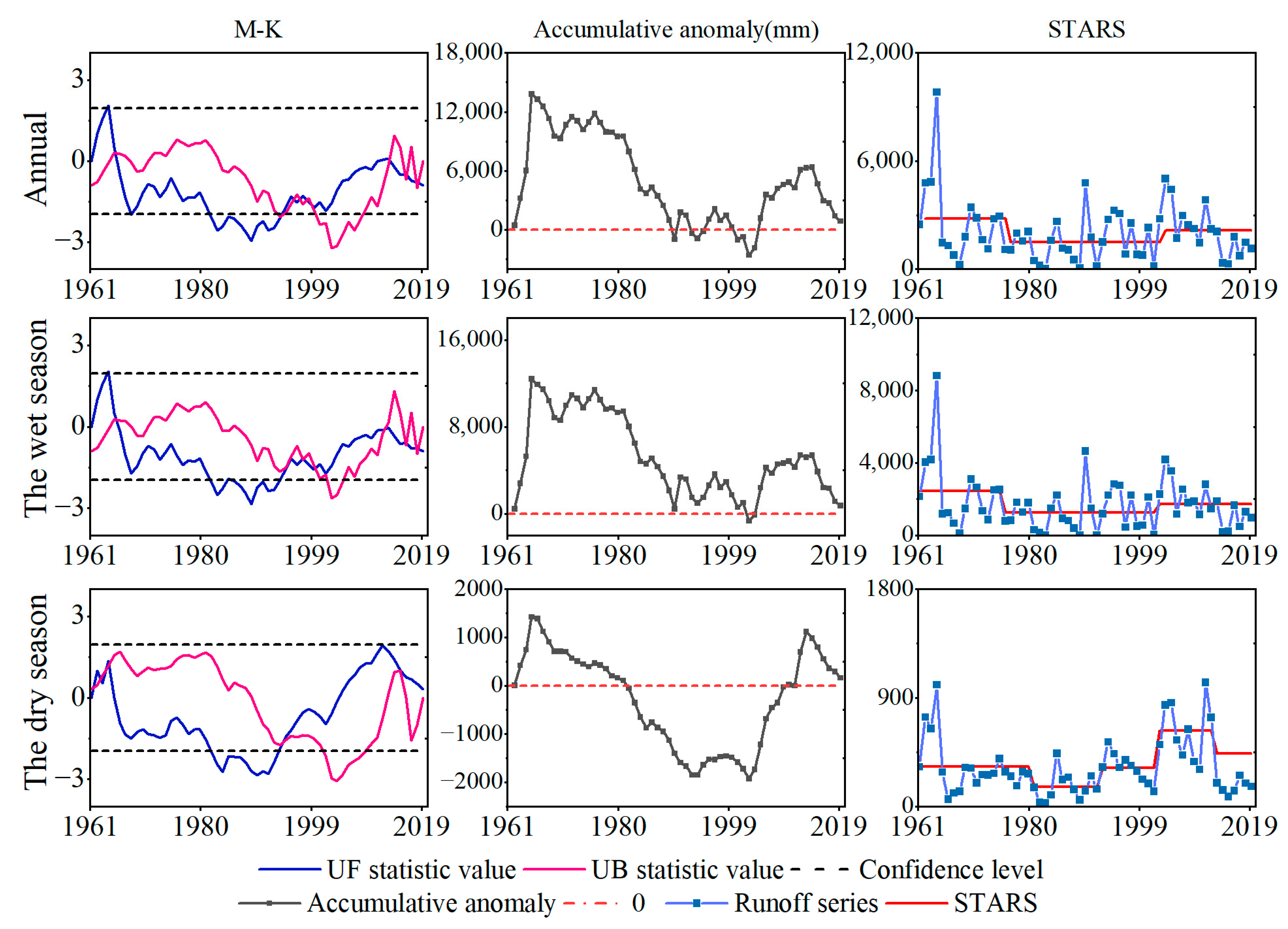
The Mann–Kendall, accumulative anomaly, STARS, and Pettitt methods were used to identify mutations in runoff series data from the hydrological stations at Laiwu, Beiwang, Dawenkou, and Daicunba in the Dawen River Basin.
- (1)
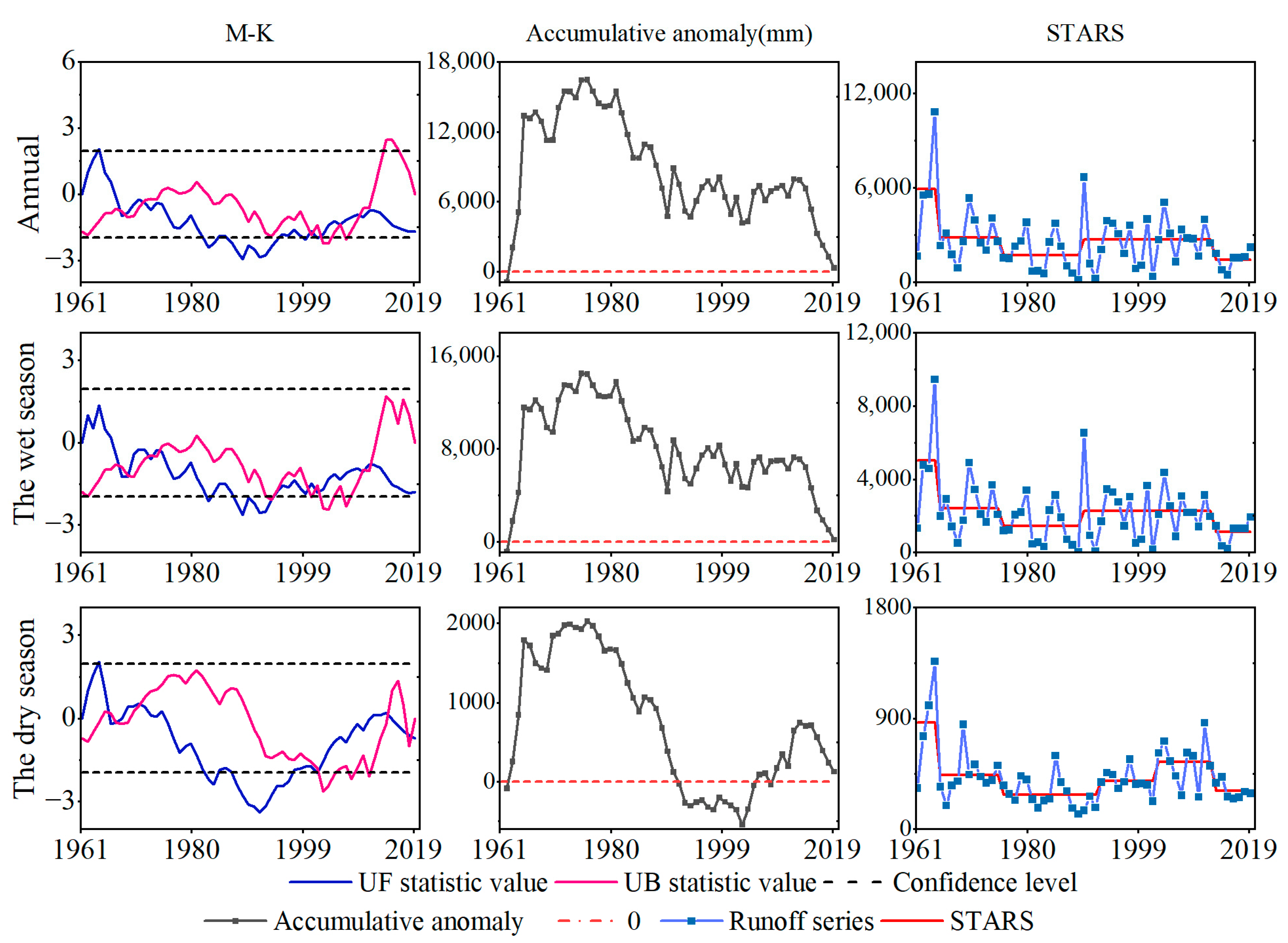
- Runoff at Laiwu Hydrological Station (Figure 6)
Interannual runoff: Based on the M-K test, there were multiple intersections of the UF and UB statistical value curves within the confidence interval, two intersections around 1968, one in 1972, two around 2002, and one each in 2006 and 2009, respectively. The accumulative anomaly curve revealed a significant mutation in 1976 (|T| = 2.53 > T [0.05/2] = 1.64). The STARS test showed that state transitions occurred in 1964–1965, 1975–1976, 1988–1989, and 2011–2012. The Pettitt test found significant mutations around 1976 (p = 0.21 < 0.5). An analysis of the change curves for the statistical values obtained with each test method and for the mutation results, combined with the dynamics of the changes in the time series of indicators, showed that significant mutation of the interannual runoff occurred in 1976.
Wet season runoff: Based on the M-K test, there were multiple intersections of the UF and UB statistical value curves within the confidence interval: two intersections around 1968, two around 1973, one in 1994, and two around 2002. The accumulative anomaly curve revealed a significant mutation in 1975 (|T| = 2.63 > T [0.05/2] = 1.64). The results of the STARS test showed that state transitions occurred in 1964–1965, 1975–1976, 1989–1990, and 2012–2013. The Pettitt test showed significant mutations around 1975 (p = 0.23 < 0.5). An analysis of the change curves for the statistical values obtained with each test method and for the mutation results, combined with the dynamics of the changes in the time series of indicators, showed that significant mutation in the wet season runoff occurred in 1976.
Dry season runoff: Based on the M-K test, there were multiple intersections of the UF and UB statistical value curves within the confidence interval: two intersections around 1968, one in 1971, two around 2002, and one in 2014. The accumulative anomaly curve revealed a significant mutation in 1976 (|T| = 2.68 > T [0.05/2] = 1.64). The results of the STARS test show that state transitions occurred in 1964–1965, 1975–1976, 1989–1990, and 2012–2013. The Pettitt test revealed significant mutations around 1976 (p = 0.24 < 0.5). An analysis of the change curves for the statistical values obtained by each test method and for the mutation results, combined with the dynamics of the changes in the time series of indicators, showed that a significant mutation in the dry season runoff occurred in 1976.
- (2)
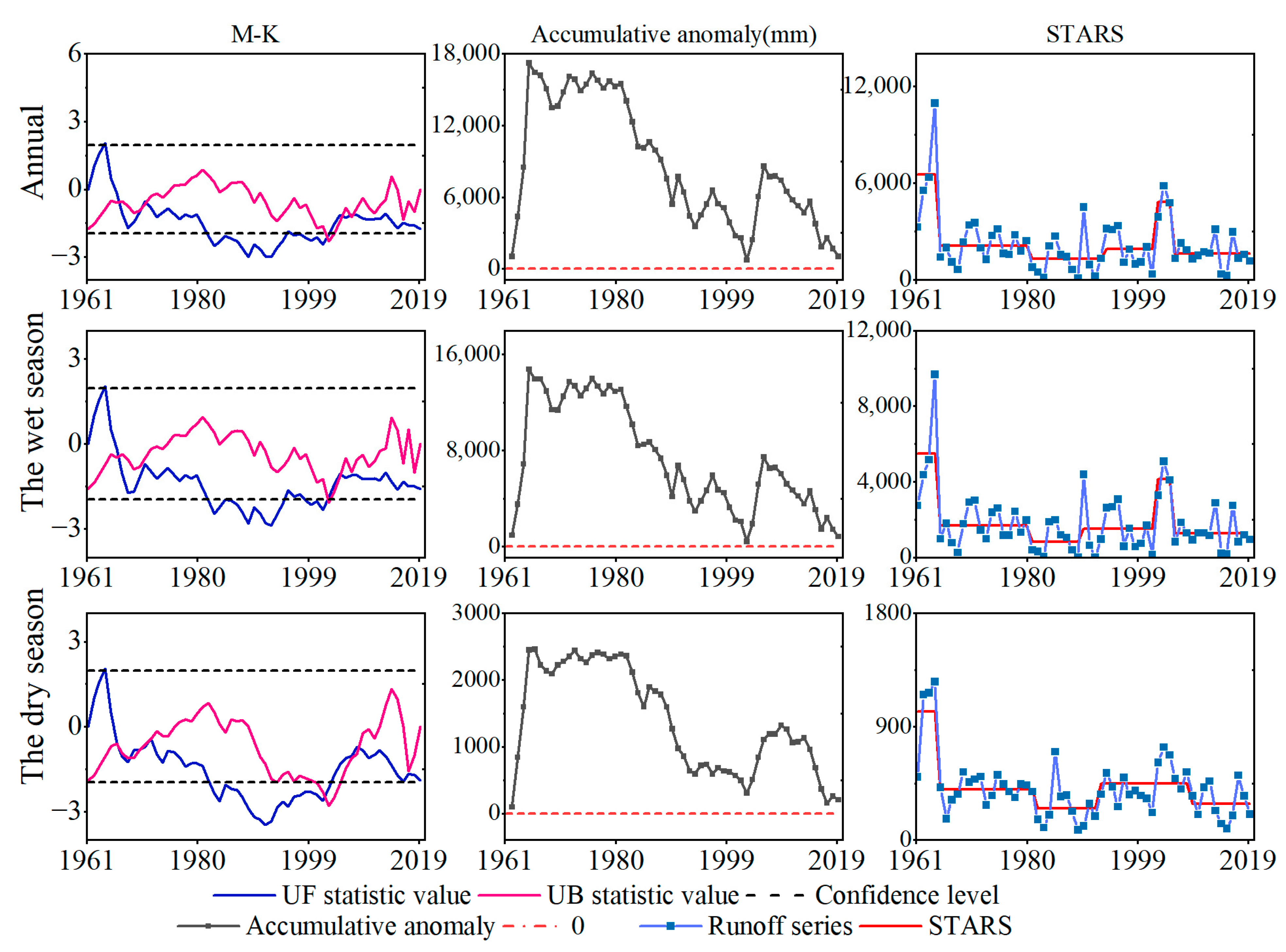
- Runoff at Beiwang Hydrological Station (Figure 7)
Interannual runoff: As shown the M-K test, there were multiple intersections of the UF and UB statistical value curves within the confidence interval: two intersections around 1966, two around 1970, and two around 2006. The accumulative anomaly curve revealed a significant mutation in 1965 (|T| = 4.76 > T [0.05/2] = 1.64), whereby a jump point was formed due to the heavy precipitation in 1964, removing the unusually large water surplus in 1964, along with a mutation point in 1980. The results of the STARS test showed that state transitions occurred in 1964–1965, 1979–1980, and 2003–2004. The Pettitt test revealed significant mutations around 1980 (p = 0.14 < 0.5). An analysis of the change curves for the statistical values obtained by each test method and for the mutation results, combined with the dynamics of the changes in the time series of indicators, determined that a significant mutation in interannual runoff occurred in 1980.
Wet season runoff: Based on the M-K test, there were multiple intersections of the UF and UB statistical value curves within the confidence interval: one intersection in 1967, one in 1972, and two around 2004. The accumulative anomaly curve test revealed a significant mutation in 1965 (|T| = 4.38 > T [0.05/2] = 1.64). A jump point formed due to the occurrence of heavy precipitation in 1964, removing the unusually large water surplus in 1964, along with a mutation point in 1980. The results of the STARS test showed that state transitions occurred in 1964–1965, 1975–1976, 1989–1990, and 2012–2013. The Pettitt test revealed significant mutations around 1980 (p = 0.18 < 0.5). An analysis of the change curves for the statistical values obtained by each test method and for the mutation results, combined with the dynamics of change in the time series of indicators, determined that a significant mutation in wet season runoff occurred in 1980.
Dry season runoff: Based on the M-K test, there were multiple intersections of the UF and UB statistical value curves within the confidence interval: four intersections from 1965 to 1973 and two in 2008. The accumulative anomaly curve test revealed a significant mutation in 1966 (|T| = 4.47 > T [0.05/2] = 1.64), whereby a jump point was formed due to the occurrence of large precipitation in 1964, removing the unusually large water surplus in 1964, along with a mutation point in 1980. The results of the STARS test showed that state transitions occurred in 1964–1965, 1975–1976, 1989–1990, and 2012–2013. The Pettitt test revealed significant mutations around 1980 (p = 0.11 < 0.5). An analysis of the change curves for the statistical values obtained by each test method and for the mutation results, combined with the dynamics of the changes in the time series of indicators, determined that a significant mutation in the dry season runoff occurred in 1980.
- (3)
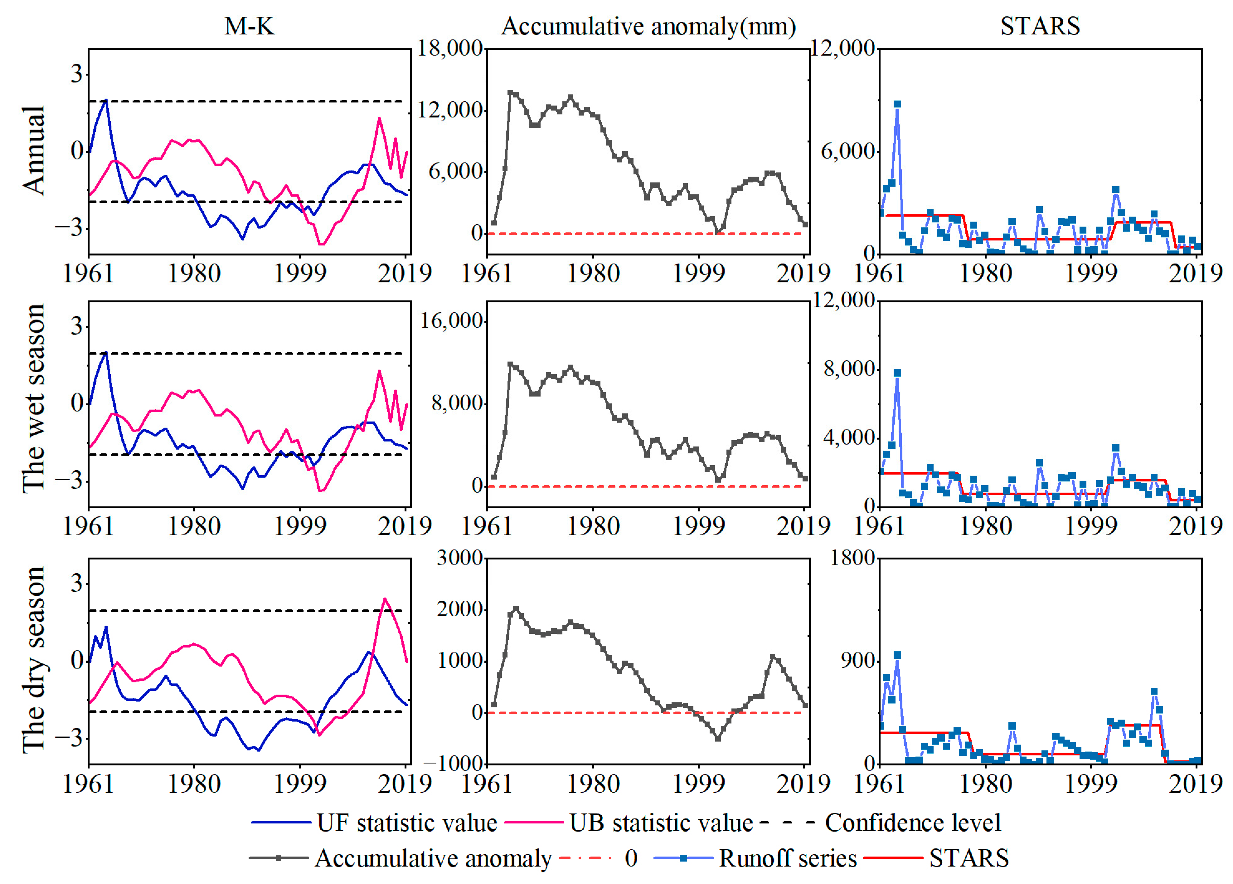
- Runoff at Dawenkou Hydrological Station (Figure 8)
Interannual runoff: Based on the M-K test, there were multiple intersections of the UF and UB statistical value curves within the confidence interval: one intersection in 1965, and five from 1994 to 2001. The accumulative anomaly curve test revealed a significant mutation in 1965 (|T| = 4.07 > T [0.05/2] = 1.64), whereby a jump point was formed due to the occurrence of heavy precipitation in 1964, removing the unusually large water surplus in 1964, along with a mutation point in 1976. The results of the STARS test showed that state transitions occurred in 1975–1976 and 2002–2003. The Pettitt test revealed significant mutations around 1975 (p = 0.39 < 0.5). An analysis of the change curves of statistical values obtained by each test method and the mutation results, combined with the dynamics of the changes in the time series of indicators, determined that a significant mutation in the interannual runoff occurred in 1976.
Wet season runoff: Based on the M-K test, there were multiple intersections of the UF and UB statistical value curves within the confidence interval: one in 1965, and five from 1994 to 2001. The accumulative anomaly curve test revealed a significant mutation in 1965 (|T| = 4.05 > T [0.05/2] = 1.64), whereby a jump point was formed due to the occurrence of heavy precipitation in 1964, removing the unusually large water surplus in 1964, along with a mutation point in 1976. The results of the STARS test showed that state transitions occurred in 1975–1976 and 2002–2003. The Pettitt test revealed significant mutations around 1975 (p = 0.33 < 0.5). An analysis of the change curves for the statistical values obtained by each test method and the mutation results, combined with the dynamics of the changes in the time series of indicators, determined that a significant mutation in the wet season runoff occurred in 1975–1976.
Dry season runoff: Based on the M-K test, there were multiple intersections of the UF and UB statistical value curves within the confidence interval: three intersections from1963 to 1965, two around 1995, and one in 2015. The accumulative anomaly curve test revealed a significant mutation in 2003 (|T| = 2.19 > T [0.05/2] = 1.64). The results of the STARS test showed that state transitions occurred in 1980–1981, 1992–1993, 2002–2003, and 2012–2013. The Pettitt test revealed significant mutations around 2011 (p = 0.37 < 0.5). An analysis of the change curves for the statistical values obtained by each test method and the mutation results, combined with the dynamics of the changes in the time series of indicators, determined that a significant mutation in the dry season runoff occurred in 2003.
- (4)
- Runoff at Daicunba Hydrological Station (Figure 9)
Interannual runoff: Based on the M-K test, there were multiple intersections of the UF and UB statistical value curves within the confidence interval: one intersection in 1966 and one in 2002. The accumulative anomaly curve test revealed a significant mutation in 1965 (|T| = 5.26 > T [0.05/2] = 1.64), whereby a jump point was formed due to the occurrence of heavy precipitation in 1964, removing the unusually large water surplus in 1964, along with a mutation point in 1976. The results of the STARS test showed that state transitions occurred in 1975–1976, 2002–2003, and 2013–2014. The Pettitt test revealed significant mutations around 1975 (p = 0.18 < 0.5). An analysis of the change curves for the statistical values obtained by each test method and the mutation results, combined with the dynamics of the changes in the time series of indicators, determined that a significant mutation in interannual runoff occurred in 1975–1976.
Wet season runoff: Based on the M-K test, there were multiple intersections of the UF and UB statistical value curves within the confidence interval: one intersection in 1966, and three intersections from 2010 to 2012. The accumulative anomaly curve test revealed a significant mutation in 1965 (|T| = 4.92 > T [0.05/2] = 1.64), whereby a jump point was formed due to the occurrence of heavy precipitation in 1964, removing the unusually large water surplus in 1964, along with a mutation point in 1976. The results of the STARS test showed that state transitions occurred in 1975–1976, 2002–2003, and 2012–2013. The Pettitt test results revealed significant mutations around 1975 (p = 0.18 < 0.5). An analysis of the change curves for the statistical values obtained by each test method and the mutation results, combined with the dynamics of the changes in the time series of indicators, determined that a significant mutation in the wet season runoff occurred in 1975–1976.
Dry season runoff: Based on the M-K test, there were multiple intersections of the UF and UB statistical value curves within the confidence interval: one intersection in 1965, and one in 2013. The accumulative anomaly curve test revealed a significant mutation in 1966 (|T| = 4.73 > T [0.05/2] = 1.64). The results of the STARS test showed that state transitions occurred in 1977–1978, 2002–2003, and 2011–2012. The Pettitt test results revealed significant mutations around 2011(p = 0.08 < 0.5). An analysis of the change curves for the statistical values obtained by each test method and the mutation results, combined with the dynamics of the changes in the time series of indicators, determined that a significant mutation in the dry season runoff occurred in 2011.
The mutations of the annual runoff and wet season occurred roughly from 1975 to 1976 at four hydrological stations in the Dawen River Basin. The mutation of the dry period at the same stations occurred later than for the annual runoff and wet season, and it occurred at a later times from upstream to downstream in 1976, 1980, 2003, and 2011, respectively.
3.3. Periodic Diagnosis
A wavelet analysis was used to analyze periodic variations in runoff at Laiwu, Beiwang, Dawenkou, and Daicunba hydrological stations in the Dawen River Basin.
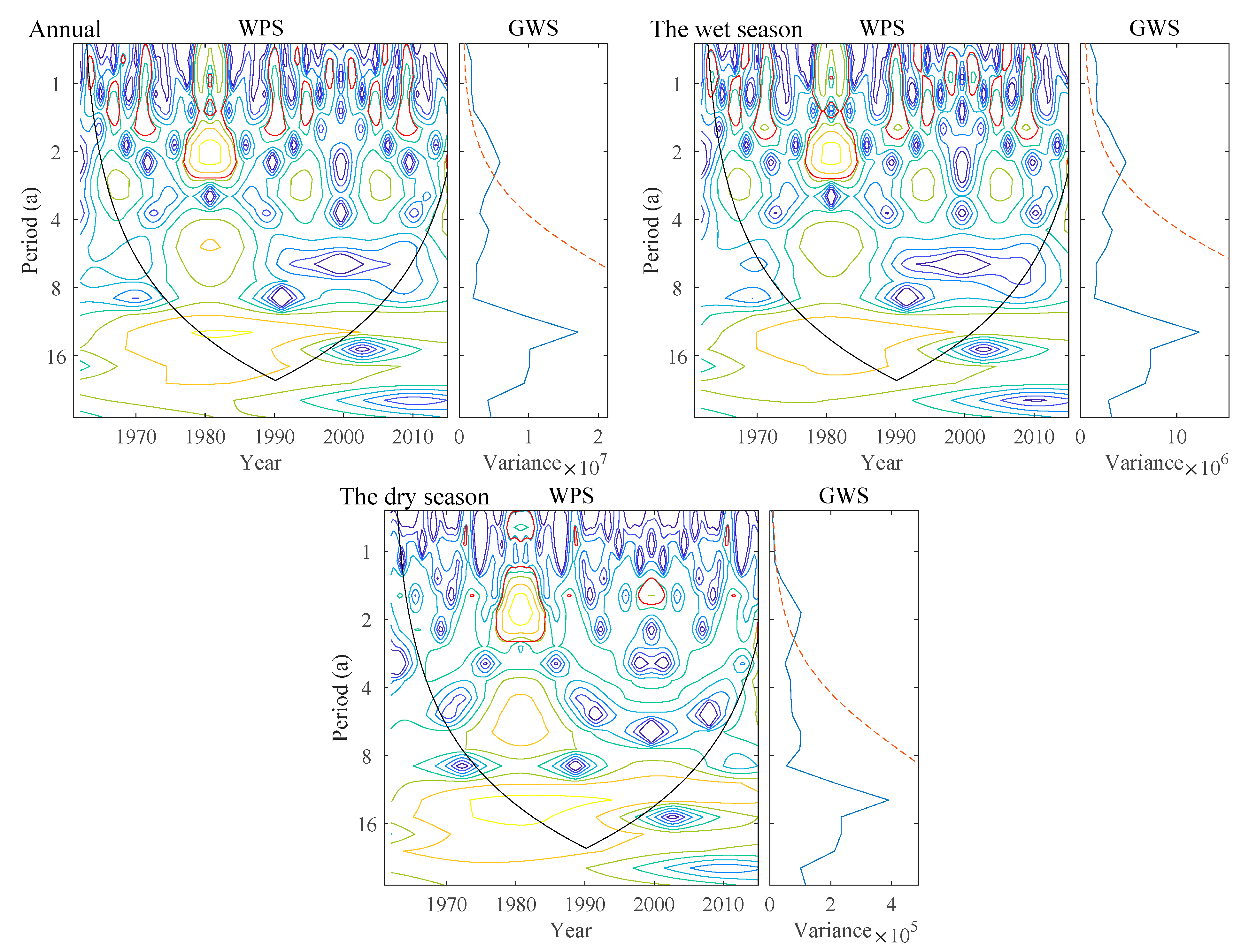
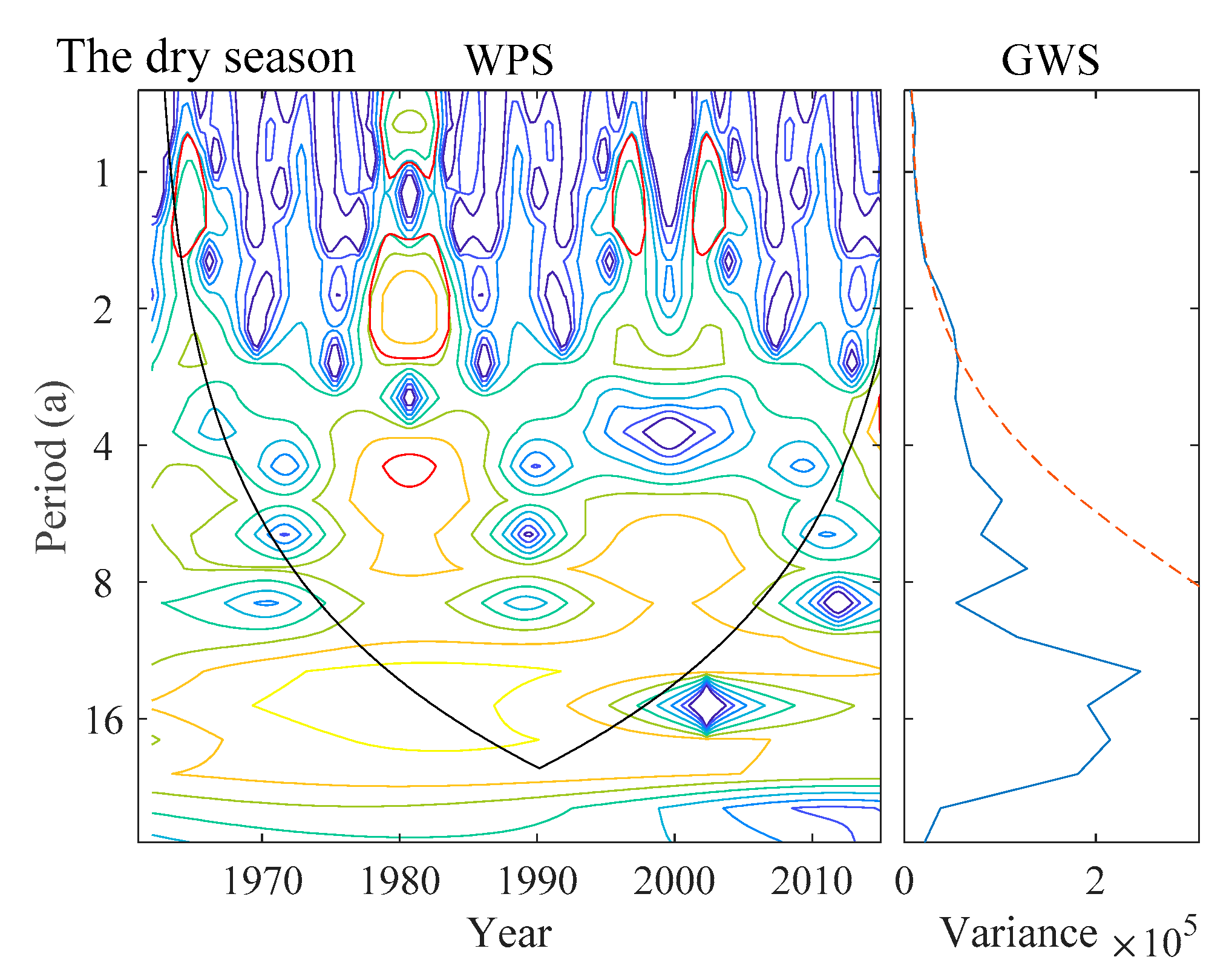
The wavelet power spectrum and global wavelet spectrum for the Laiwu hydrological station are shown in Figure 10. The oscillation periods of the interannual and wet season runoff series were generally consistent. The range of the significant period was 0.7–2.5 years, there was a main period of 2.2 years, and the variation was most significant in the period 1965–1995, during the early 21st century. Furthermore, there was a significant period of 1.1 years and non-significant periods of about 5.3 and 12.6 years. During the dry season, the significant period for the runoff ranged over 0.7–2.4 years. There was a main period of 1.9 years, and the period variation was most significant over 1976–1984. There was a significant period of 0.8 years and non-significant periods of about 12.6 and 17.8 years.
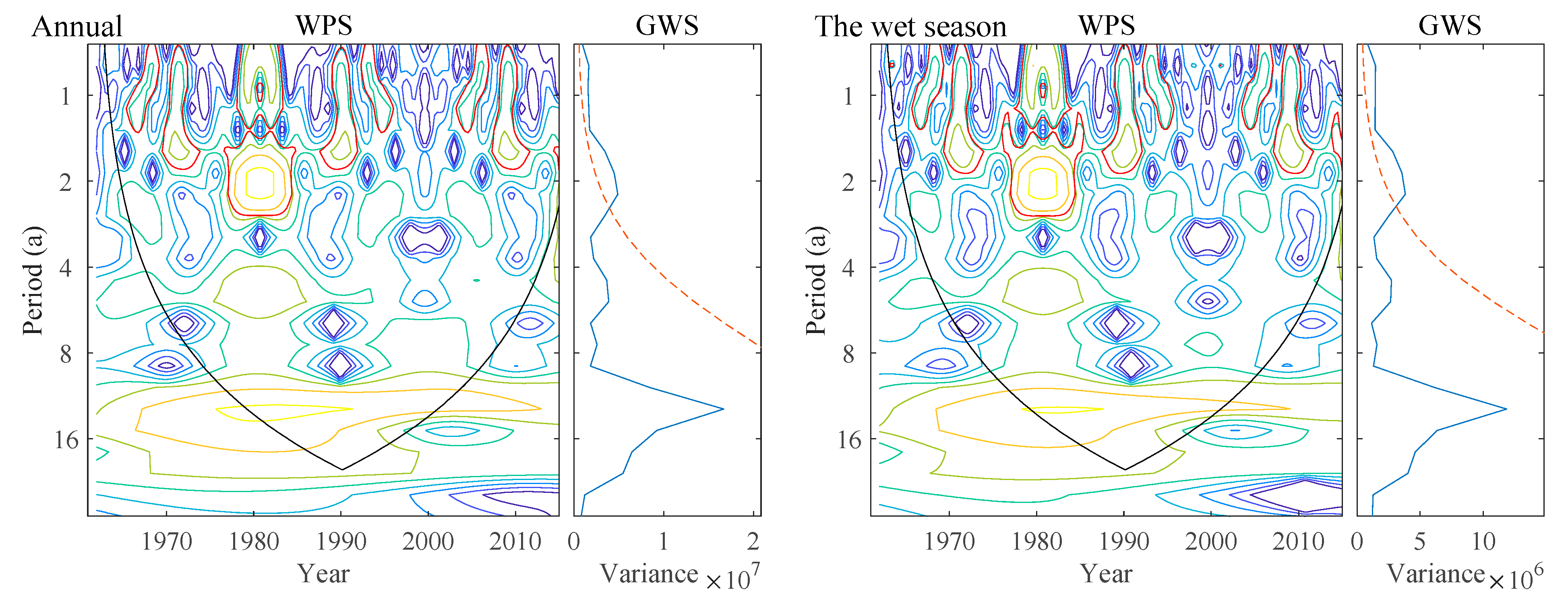
The wavelet power spectrum and global wavelet spectrum for Beiwang hydrological station are shown in Figure 11. The oscillation periods of the interannual and wet season runoff series were generally consistent. The range of the significant period range was 0.7–2.6 years, there was a main period of 2.2 years, and the variation was most significant over the period 1976–1984. Furthermore, there was a significant period of 1.1 years and non-significant periods of about 4.4, 7.5, and 12.6 years. During the dry season, the significant runoff period ranged over 1.2–2.4 years, there was a main period of 1.9 years, and the variation was most significant over the periods 1976–1984 and 1997–2001. There were non-significant periods of about 3.7, 6.3, and 12.6 years.
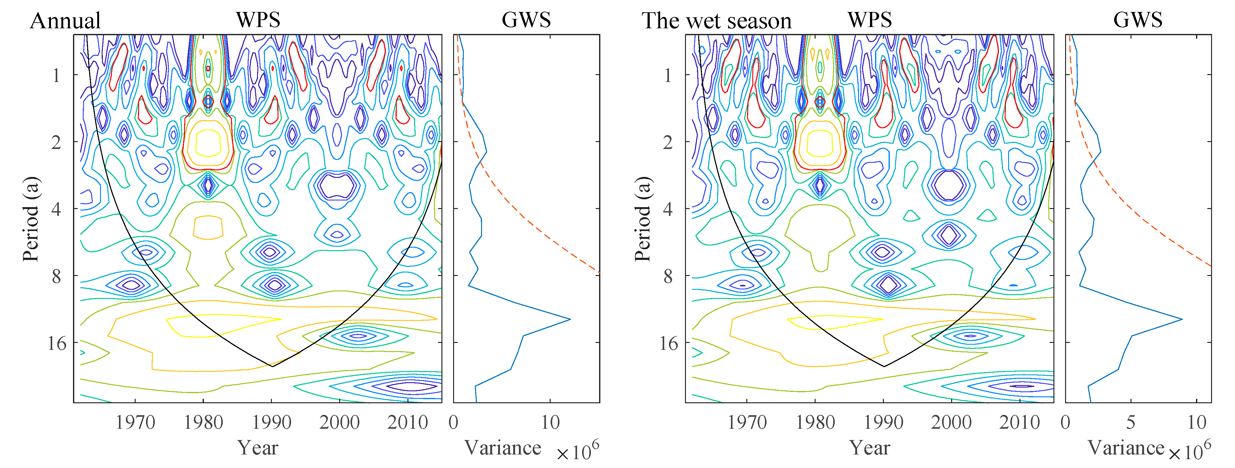
The wavelet power spectrum and global wavelet spectrum for Dawenkou hydrological station are shown in Figure 12. The oscillation periods of the interannual and wet season runoff series were generally consistent. The range of the significant period was 0.7–2.6 years, there was a main period of 2.2 years, and the variation was most significant over the period 1977–1984. Additionally, there was a significant period of 0.8 years and non-significant periods of about 5.3, 7.5, and 12.6 years. During the dry season, the significant period for the runoff ranged 0.8–2.7 years, there was a main period of 2.2 years, and the variation was most significant over the periods 1963–1967, 1976–1984, 1993–1998, and 2000–2005. There were non-significant periods of about 5.3, 7.5, and 12.6 years.
The wavelet power spectrum and global wavelet spectrum for Daicunba hydrological station are shown in Figure 13. The oscillation periods of the interannual and wet season runoff series were generally consistent. The range of the significant period was 0.7–2.5 years, there was a main period of 2.2 years, and the variation was most significant over the period 1977–1984. There were significant periods of 0.8 and 1.1 years and non-significant periods of about 5.3, 7.5, and 12.6 years. During the dry season, the significant periods for the runoff ranged 0.8–0.9 and 1.7–2.5 years, there was a main period of 2.2 years, and the variation was most significant over the period 1978–1983. There were non-significant periods of about 5.3, 7.5, 12.6, and 17.8 years.
3.4. Decomposition and Reclassification of the Dynamic Features of Runoff Sequences
The monthly runoff series for four hydrological stations, upstream to downstream of the Dawen River Basin, namely Laiwu, Beiwang, Dawenkou, and Daicunba, were decomposed and reclassified. The internal dynamic characteristics of the runoff were analyzed, and the intra-annual, interannual, and long-term trends were analyzed based on the CEEMDAN method.
- (1)
- Decomposition of runoff sequences
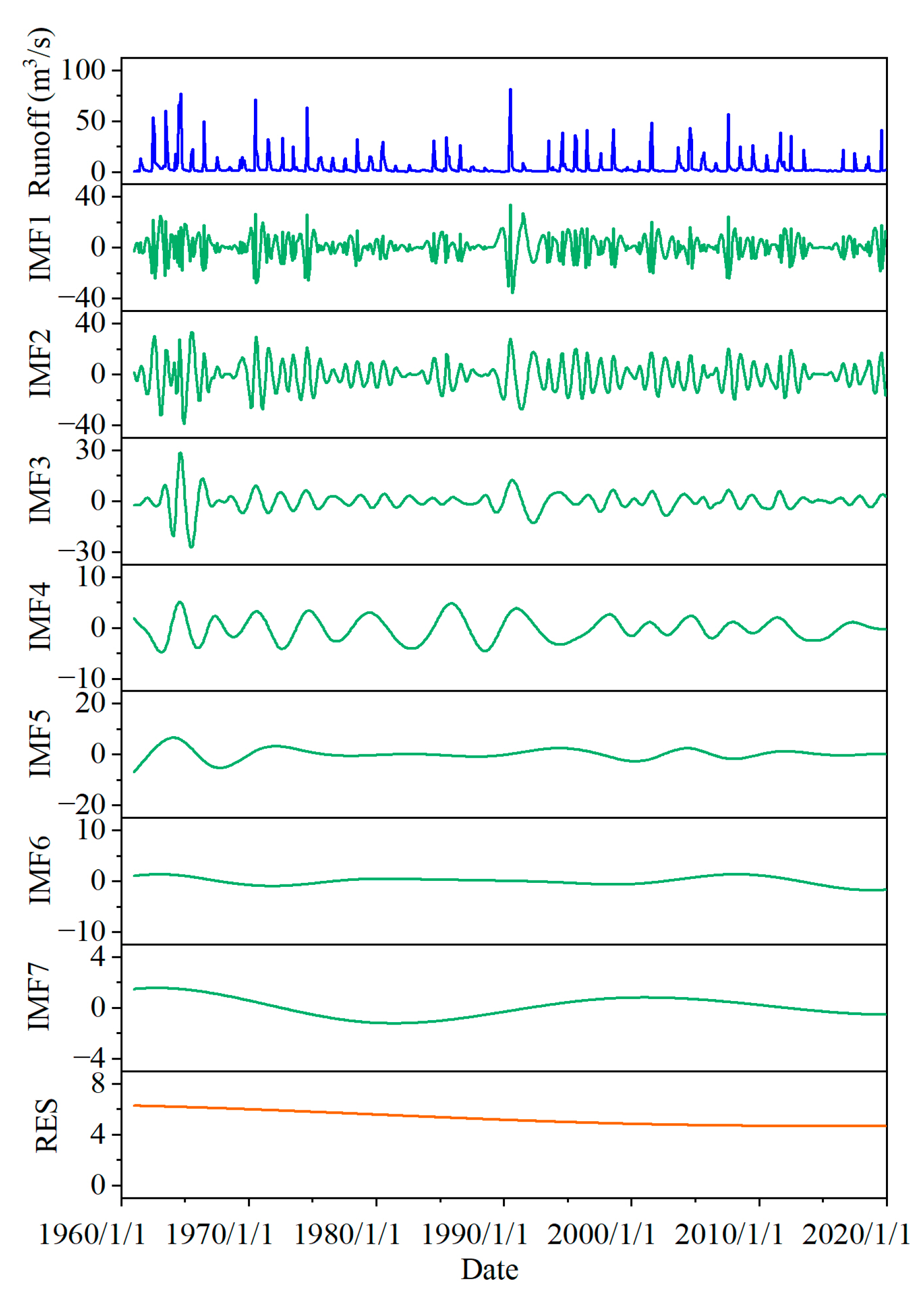
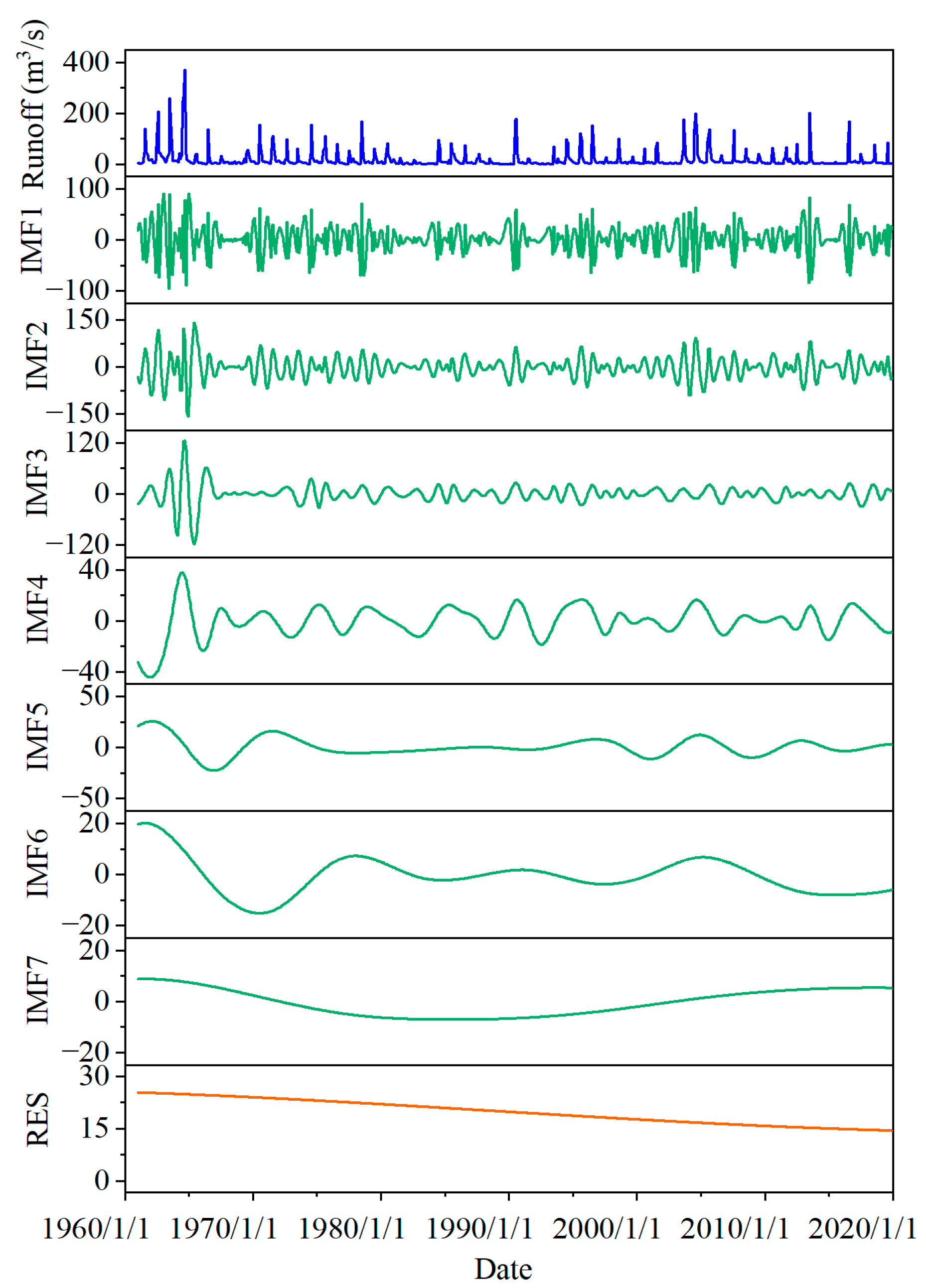
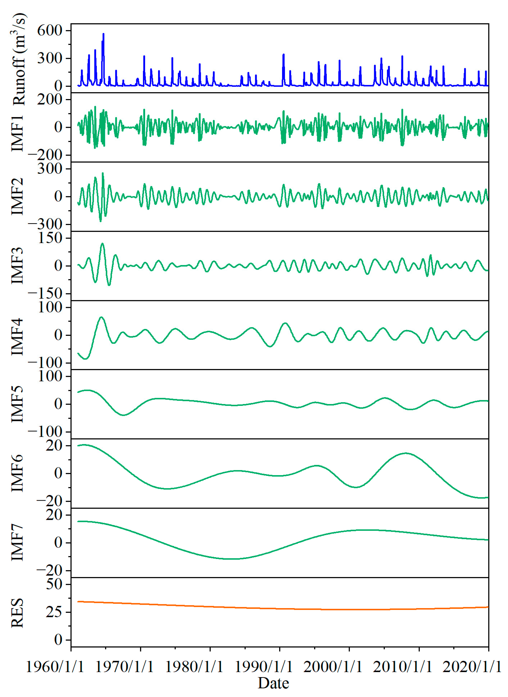
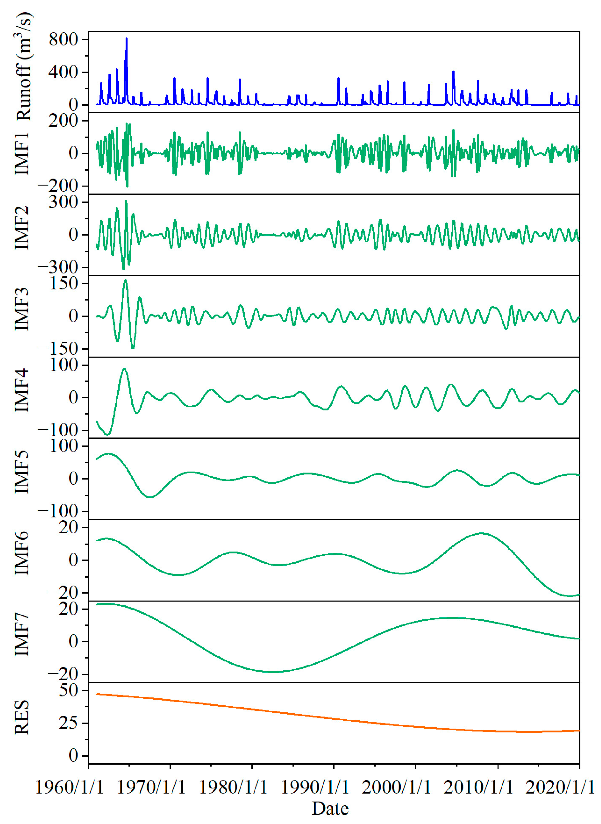
The results from decomposing IMF terms and residual terms based on the CEEMDAN method for runoff data from four hydrological stations in Laiwu, Beiwang, Dawenkou, and Daicunba are shown in Figure 14, Figure 15, Figure 16 and Figure 17. To ensure the accuracy of the results, the CEEMDAN decomposition test was run 500 times, in which the white noise coefficient was set to 0.2 to ensure that accurate decomposition data were obtained. Seven IMF terms and one residual term were obtained for the long series runoff decomposition at all four hydrological stations. The frequency and amplitude of the runoff IMF terms changed more notably from high to low frequencies, and the high frequency IMF term was closer to the characteristics of the runoff data. The frequency decreased gradually as the IMF term increased, reflecting the periodicity and tendency of the runoff data. From the upstream to downstream stations of Laiwu, Beiwang, Dawenkou, and Daicunba, the amplitude of the decomposition tended to increase with the increased runoff. This amplitude reached the maximum in the IMF2 term and then gradually decreased. The residual term of the runoff decomposition tended to decrease throughout the observation period and the amplitude was relatively weak.
- (2)
- Analysis of Characteristics
To analyze the runoff characteristics decomposed by the CEEMDAN method, several important indicators of the IMF and residual terms were analyzed in this study, including the mean period, mean, variance, percentage of variance, and Pearson correlation between IMF and residual terms and runoff series (Table 3). The results revealed that the fluctuations were more intense and the period was shorter for smaller IMF terms, while the period for each runoff decomposition term gradually increased and the data gradually stabilized as the IMF term increased. The average absolute value and variance of each IMF increased gradually with the increasing flow from upstream to downstream of the hydrological station. The variance ratio for each runoff station revealed that Laiwu and Beiwang stations had a mutation at IMF3, while Dawenkou and Daicunba had a mutation at IMF2. The IMF terms for the four runoff stations presented an increasing trend from IMF1, reaching the maximum at IMF2 and then decreasing rapidly.
- (3)
- Reclassification
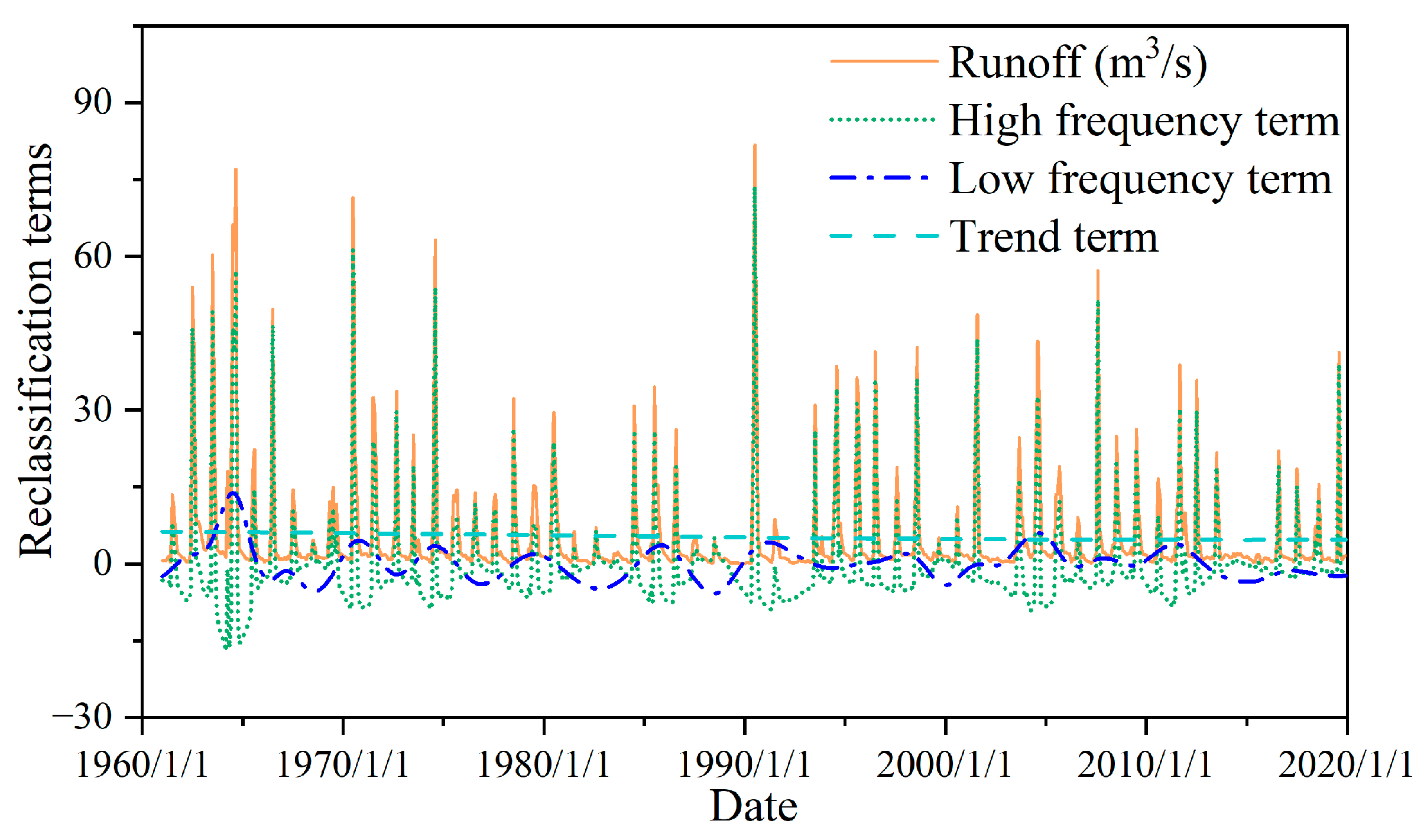
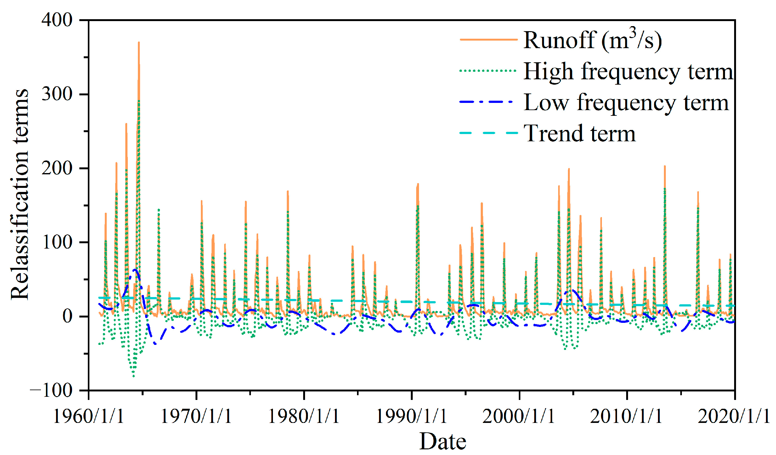
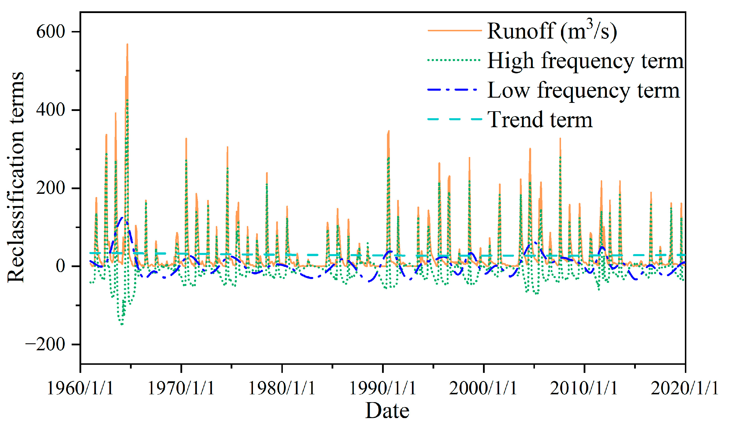
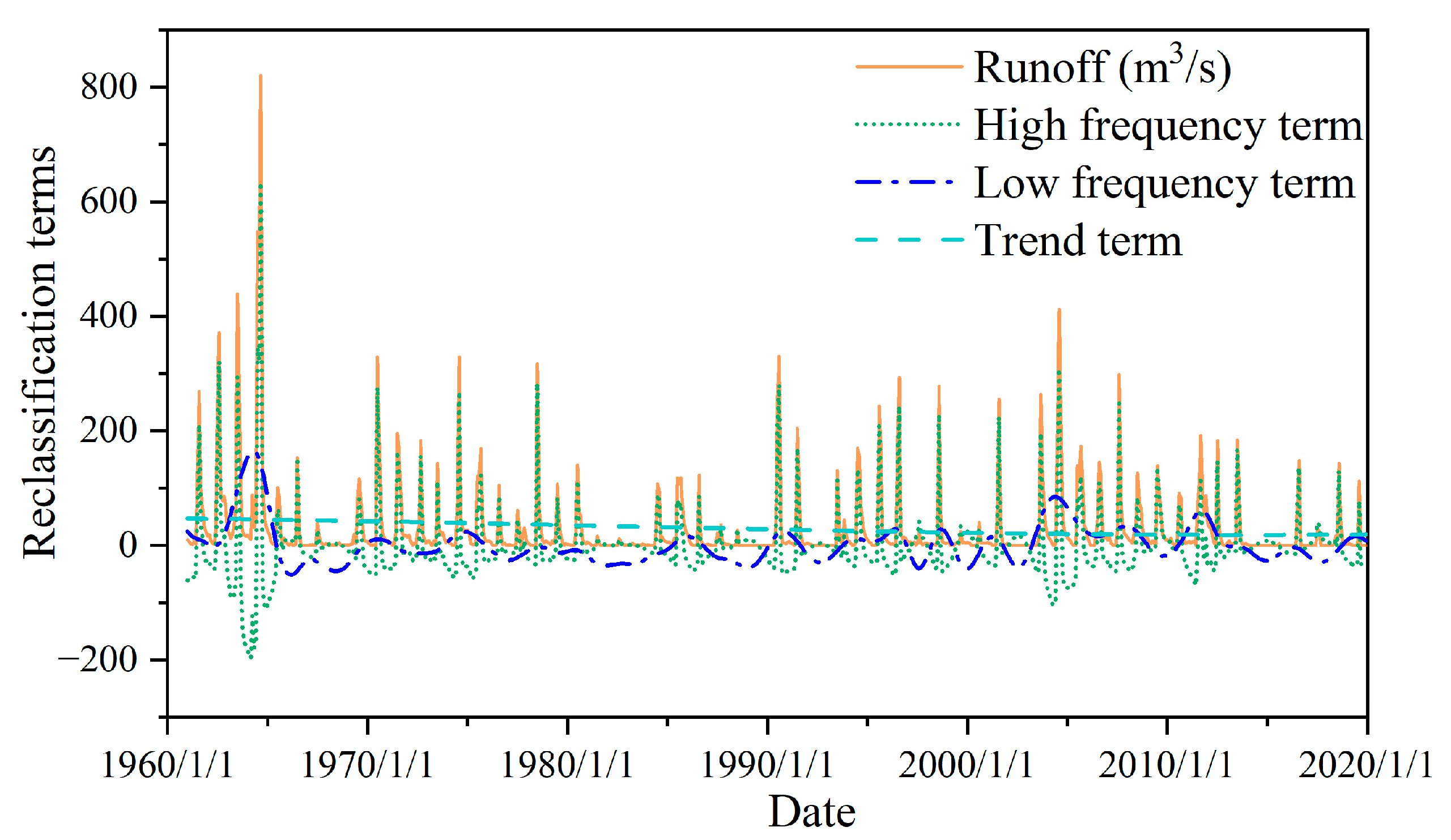
The decomposition of the runoff by the CEEMDAN method can capture more dynamic information on the characteristics of the runoff; however, too many decomposition terms may also impact analyses on the dynamic characteristics of runoff. To overcome the multiple IMF terms in the runoff data decomposition, this study integrated the percentage of variance and Pearson correlation mutation points for classification. Combined with the characteristic analysis of the IMF terms, the terms for IMF1–IMF3 at Laiwu and Beiwang stations were reclassified as high-frequency terms, reflecting the intra-annual fluctuation in runoff. The terms for IMF4-IMF7 were reclassified as low-frequency terms, reflecting the interannual fluctuations in runoff. The residual term represents the long-term tendency of the runoff. The terms for IMF1 and IMF2 at Dawenkou and Daicunba stations were reclassified as high-frequency terms, the terms for IMF3–IMF7 were reclassified as low-frequency terms, and the residual terms were classified as trend terms (Figure 18, Figure 19, Figure 20 and Figure 21).
The results confirmed that the high-frequency term for the runoff data decomposition (i.e., the intra-annual fluctuation term) had a stronger fluctuation frequency, which was similar to the fluctuation frequency of the runoff series. The tendency of the low-frequency term (i.e., interannual fluctuation term) of the runoff data decomposition term was similar to the increasing and decreasing trends of the runoff interannual. Additionally, the analysis of the reclassified terms revealed (Table 4) that the periodicity of the intra-annual fluctuation terms was about 6.10–6.62 months, indicating that the intra-annual runoff fluctuation had a periodicity of about half a year (0.51–0.55 years), the interannual fluctuation had a periodicity of about 27.23–18.63 months (2.26–1.55 years), and the period gradually shortened from the upstream to downstream hydrological stations.
4. Conclusions
In this study, the trends, mutations, and periodicity of the runoff in the Dawen River Basin were analyzed, and the runoff was decomposed and reclassified. The dynamic evolution of the runoff under changing environments was explored using various methods.
- (1)
- Tendency analysis
The intra-annual distribution of the runoff in the Dawen River Basin was uneven. The annual runoff, the wet season runoff, and the dry season runoff for all hydrological stations presented a downward trend, and the runoff decreased continuously from upstream to downstream. The runoff in the early years of the study period (1961–1969) was relatively high in each chronological analysis. The dynamics and magnitude of the annual runoff and the wet season runoff remained similar, while the dry season runoff rates differed. The changes in runoff indicated that under environments of climate change, human activities have a greater impact on runoff.
- (2)
- Mutation analysis
From upstream to downstream, the annual, wet season, and dry season runoff for Laiwu hydrological station showed mutations in 1975–1976. The annual runoff, wet season, and dry season runoff at Beiwang Hydrological Station mutated in 1980. The annual and wet season runoff at Dawenkou Hydrological Station mutated in 1975–1976, while the dry season runoff mutated in 2003. The annual and wet season runoff at Daicunba Hydrological Station mutated in 1975–1976, while the dry season runoff mutated in 2011. In summary, runoff mutation in the Dawen River Basin occurred in 1975–1976.
- (3)
- Periodic analysis
The significant periods for annual, wet season, and dry season runoff at all hydrological stations was 0.7–2.7 years. The main period of annual and wet season runoff for all hydrological stations was 2.2 years, with more intense vibration observed over 1977–1984. The main period of dry season runoff at the Laiwu and Beiwang hydrologist stations was 1.9 years, while that at the Dawenkou and Daicunba hydrologist stations was 2.2 years, with the most sever oscillations observed over 1978–1983.
- (4)
- Decomposition and reclassification of runoff
Using the CEEMDAN method for runoff decomposition and reclassification, the runoff decomposition high-frequency term (intra-annual fluctuation term) had a strong fluctuation frequency with an intra-annual period of 0.51–0.55 years. The trend for the low-frequency term (i.e., interannual fluctuation term) was similar to that for increasing and decreasing annual runoff, with an interannual fluctuation term of 1.55–2.26 years. The trend term for the runoff data decomposition term decreased throughout the monitoring period and gradually stabilized at the end of the monitoring period, and the period gradually decreased from upstream to downstream.
The impacts of climate change and human activities have been accompanied by significant trend changes in hydrological elements in temporal, spatial, and quantitative terms. The frequent occurrence of extreme hydrological events and the increasing demand for regional water security and water resource management have placed more demand on regional water cycle research. In practical applications, it is necessary to enhance the preparation and evaluation of hydro-meteorological element observation data and spatial and temporal distribution data, to select effective analysis methods to improve the accuracy of the runoff evolution characteristic detection process, and to further deepen the understanding of the spatial and temporal variability characteristics of runoff. After clarifying the evolution pattern of runoff under changing environments, further research on the driving mechanism of the runoff evolution should be carried out.
Author Contributions
Methodology, X.Y.; software, X.Y.; investigation, J.L. (Jian Liu) and Y.L.; resources, J.L. (Jian Liu) and M.W.; writing—original draft preparation, X.Y.; writing—review and editing, X.Y.; visualization, J.X. and J.L. (Jiake Li). All authors have read and agreed to the published version of the manuscript.
Funding
This research received no external funding.
Data Availability Statement
The data used in this paper were from the Shandong Provincial Hydrological Bureau. You can apply for data from Shandong Provincial Hydrological Bureau to get the required data.
Acknowledgments
We thank editage (www.editage.cn, accessed on 1 January 2023) for its linguistic during the preparation of this manuscript. This paper was financially supported by “Simulation and Regulation of Water and Salt Processes in the Irrigation Districts of the Lower Yellow River Basin under the High-Quality Development” project supported by National Natural Science Foundation of China (No. U22A20555), the National Natural Science Foundation for Yong Scholars of China (No. 41501053), and the National Natural Science Foundation of China (General Program) (No. 41877159). We would like to thank the Shandong Provincial Hydrological Bureau for providing the runoff data.
Conflicts of Interest
The authors declare no conflict of interest.
References
- IPCC. Climate Change 2007—The Physical Science Basis: Working Group I Contribution to the Fourth Assessment Report of the IPCC; Cambridge University Press: Cambridge, UK, 2007. [Google Scholar]
- Brown, A.E.; Zhang, L.; McMahon, T.A.; Western, A.W.; Vertessy, R.A. A Review of Paired Catchment Studies for Determining Changes in Water Yield Resulting from Alterations in Vegetation. J. Hydrol. 2005, 310, 28–61. [Google Scholar] [CrossRef]
- Wang, S.; Zhang, Z.; McVicar, T.R.; Guo, J.; Tang, Y.; Yao, A. Isolating the Impacts of Climate Change and Land Use Change on Decadal Streamflow Variation: Assessing Three Complementary Approaches. J. Hydrol. 2013, 507, 63–74. [Google Scholar] [CrossRef]
- The Water Cycle|U.S. Geological Survey. Available online: https://www.usgs.gov/special-topics/water-science-school/science/water-cycle# (accessed on 12 November 2022).
- de Oliveira Serrão, E.A.; Silva, M.T.; Ferreira, T.R.; de Ataide, L.C.P.; dos Santos, C.A.; de Lima, A.M.M.; da Silva, V.D.P.R.; de Sousa, F.D.A.S.; Gomes, D.J.C. Impacts of Land Use and Land Cover Changes on Hydrological Processes and Sediment Yield Determined Using the SWAT Model. Int. J. Sediment Res. 2022, 37, 54–69. [Google Scholar] [CrossRef]
- Chanapathi, T.; Thatikonda, S. Investigating the Impact of Climate and Land-Use Land Cover Changes on Hydrological Predictions over the Krishna River Basin under Present and Future Scenarios. Sci. Total Environ. 2020, 721, 137736. [Google Scholar] [CrossRef]
- Guo, Y.; Li, Z.; Amo-Boateng, M.; Deng, P.; Huang, P. Quantitative Assessment of the Impact of Climate Variability and Human Activities on Runoff Changes for the Upper Reaches of Weihe River. Stoch. Environ. Res. Risk Assess. 2014, 28, 333–346. [Google Scholar] [CrossRef]
- Piao, S.; Ciais, P.; Huang, Y.; Shen, Z.; Peng, S.; Li, J.; Zhou, L.; Liu, H.; Ma, Y.; Ding, Y.; et al. The Impacts of Climate Change on Water Resources and Agriculture in China. Nature 2010, 467, 43–51. [Google Scholar] [CrossRef] [PubMed]
- Vörösmarty, C.J.; Green, P.; Salisbury, J.; Lammers, R.B. Global Water Resources: Vulnerability from Climate Change and Population Growth. Science 2000, 289, 284–288. [Google Scholar] [CrossRef]
- Li, L.; Ni, J.; Chang, F.; Yue, Y.; Frolova, N.; Magritsky, D.; Borthwick, A.G.L.; Ciais, P.; Wang, Y.; Zheng, C.; et al. Global Trends in Water and Sediment Fluxes of the World’s Large Rivers. Sci. Bull. 2020, 65, 62–69. [Google Scholar] [CrossRef] [PubMed]
- Wang, S.; McVicar, T.R.; Zhang, Z.; Brunner, T.; Strauss, P. Globally Partitioning the Simultaneous Impacts of Climate-Induced and Human-Induced Changes on Catchment Streamflow: A Review and Meta-Analysis. J. Hydrol. 2020, 590, 125387. [Google Scholar] [CrossRef]
- Labat, D.; Goddéris, Y.; Probst, J.L.; Guyot, J.L. Evidence for Global Runoff Increase Related to Climate Warming. Adv. Water Resour. 2004, 27, 631–642. [Google Scholar] [CrossRef]
- Duan, K.; Sun, G.; McNulty, S.G.; Caldwell, P.V.; Cohen, E.C.; Sun, S.; Aldridge, H.D.; Zhou, D.; Zhang, L.; Zhang, Y. Future Shift of the Relative Roles of Precipitation and Temperature in Controlling Annual Runoff in the Conterminous United States. Hydrol. Earth Syst. Sci. 2017, 21, 5517–5529. [Google Scholar] [CrossRef]
- Tan, X.; Gan, T.Y. Contribution of Human and Climate Change Impacts to Changes in Streamflow of Canada. Sci. Rep. 2015, 5, 17767. [Google Scholar] [CrossRef] [PubMed]
- Wang, Y.; Wang, S.; Wang, C.; Zhao, W. Runoff Sensitivity Increases with Land Use/Cover Change Contributing to Runoff Decline across the Middle Reaches of the Yellow River Basin. J. Hydrol. 2021, 600, 126536. [Google Scholar] [CrossRef]
- Zhang, X.; Harvey, K.D.; Hogg, W.D.; Yuzyk, T.R. Trends in Canadian Streamflow. Water Resour. Res. 2001, 37, 987–998. [Google Scholar] [CrossRef]
- Kahya, E.; Kalayci, S. Trend Analysis of Streamflow in Turkey. J. Hydrol. 2004, 289, 128–144. [Google Scholar] [CrossRef]
- Hamed, K.H. Trend Detection in Hydrologic Data: The Mann–Kendall Trend Test under the Scaling Hypothesis. J. Hydrol. 2008, 349, 350–363. [Google Scholar] [CrossRef]
- Zhang, J.; Wang, G.; Jin, J.; He, R.; Liu, C. Evolution and Variation Characteristics of the Recorded Runoff for the Major Rivers in China during 1956–2018. Adv. Water Sci. 2020, 31, 153–161. [Google Scholar] [CrossRef]
- Fleming, S.W.; Marsh Lavenue, A.; Aly, A.H.; Adams, A. Practical Applications of Spectral Analysis of Hydrologic Time Series. Hydrol. Process. 2002, 16, 565–574. [Google Scholar] [CrossRef]
- Padmanabhan, G.; Rao, A.R. Maximum Entropy Spectral Analysis of Hydrologic Data. Water Resour. Res. 1988, 24, 1519–1533. [Google Scholar] [CrossRef]
- Sang, Y.F.; Wang, Z.; Liu, C. Period Identification in Hydrologic Time Series Using Empirical Mode Decomposition and Maximum Entropy Spectral Analysis. J. Hydrol. 2012, 424, 154–164. [Google Scholar] [CrossRef]
- Coulibaly, P.; Burn, D.H. Wavelet Analysis of Variability in Annual Canadian Streamflows. Water Resour. Res. 2004, 40, 1–14. [Google Scholar] [CrossRef]
- Labat, D. Recent Advances in Wavelet Analyses: Part 1. A Review of Concepts. J. Hydrol. 2005, 314, 275–288. [Google Scholar] [CrossRef]
- Sang, Y.F.; Sun, F.; Singh, V.P.; Xie, P.; Sun, J. A Discrete Wavelet Spectrum Approach for Identifying Non-Monotonic Trends in Hydroclimate Data. Hydrol. Earth Syst. Sci. 2018, 22, 757–766. [Google Scholar] [CrossRef]
- Huang, N.E.; Shen, Z.; Long, S.R.; Wu, M.C.; Shih, H.H.; Yen, N.; Tung, C.C.; Liu, H.H. The Empirical Mode Decomposition and the Hilbert Spectrum for Nonlinear and Non-Stationary Time Series Analysis. Proc. R. Soc. A 1996, 454, 903–995. [Google Scholar] [CrossRef]
- Sang, Y.F.; Wang, Z.; Liu, C. Comparison of the MK Test and EMD Method for Trend Identification in Hydrological Time Series. J. Hydrol. 2014, 510, 293–298. [Google Scholar] [CrossRef]
- Marden, J.I.; Kendall, M.; Gibbons, J.D. Rank Correlation Methods (5th Ed.). J. Am. Stat. Assoc. 1992, 87, 108. [Google Scholar] [CrossRef]
- Mann, H.B. Mann Nonparametric Test against Trend. Econometrica 1945, 13, 245–259. [Google Scholar] [CrossRef]
- Burn, D.H.; Hag Elnur, M.A. Detection of Hydrologic Trends and Variability. J. Hydrol. 2002, 255, 107–122. [Google Scholar] [CrossRef]
- Pettitt, A.N. A Non-Parametric Approach to the Change-Point Problem. Applied statistics. 1979, 28, 126–135. [Google Scholar] [CrossRef]
- Rodionov, S.N. A Sequential Algorithm for Testing Climate Regime Shifts. Geophys. Res. Lett. 2004, 31, 1–4. [Google Scholar] [CrossRef] [Green Version]
- Rodionov, S.N. A Comparison of Two Methods for Detecting Abrupt Changes in the Variance of Climatic Time Series. Adv. Stat. Climatol. Meteorol. Oceanogr. 2016, 2, 1–32. [Google Scholar] [CrossRef]
- Gilani, M.M.; Tigabu, M.; Liu, B.; Farooq, T.H.; Rashid, M.H.U.; Ramzan, M.; Ma, X. Seed Germination and Seedling Emergence of Four Tree Species of Southern China in Response to Acid Rain. J. For. Res. 2021, 32, 471–481. [Google Scholar] [CrossRef]
- Wang, W.; Ding, J.; Li, Y. Hydrology Wavelet Analysis; Chemical Industry Press: Beijing, China, 2005; ISBN 7502568581. [Google Scholar]
- Yeh, J.R.; Shieh, J.S.; Huang, N.E. Complementary Ensemble Empirical Mode Decomposition: A Novel Noise Enhanced Data Analysis Method. Adv. Adapt Data Anal. 2010, 2, 135–156. [Google Scholar] [CrossRef]
- Wu, Z.; Huang, N.E. Ensemble Empirical Mode Decomposition: A Noise-Assisted Data Analysis Method. Adv. Adapt Data Anal. 2009, 1, 1–41. [Google Scholar] [CrossRef]
- Torres, M.E.; Colominas, M.A.; Schlotthauer, G.; Flandrin, P. A Complete Ensemble Empirical Mode Decomposition with Adaptive Noise. In Proceedings of the 2011 IEEE International Conference on Acoustics, Speech and Signal Processing (ICASSP), Prague, Czech Republic, 22–27 May 2011; pp. 4144–4147, ISBN 9781457705397. [Google Scholar]
Figure 1.
An overview map of the Daven River Basin.

Figure 2.
The integrated framework of the methods used to analyze runoff characteristics.

Figure 3.
The annual distribution of the runoff in the Dawen River Basin.

Figure 4.
The trend analysis for annual runoff in the Dawen River Basin.

Figure 5.
The decadal runoff anomaly map of the Dawen River Basin.

Figure 6.
The mutation analysis of the runoff at Laiwu station.

Figure 7.
The mutation analysis of the runoff at Beiwang station.

Figure 8.
The mutation analysis of the runoff at Dawenkou station.

Figure 9.
The mutation analysis of the runoff at Daicunba station.

Figure 10.
The runoff wavelet power spectrum and global wavelet spectrum for Laiwu station.

Figure 11.
The runoff wavelet power spectrum and global wavelet spectrum for Beiwang station.

Figure 12.
The runoff wavelet power spectrum and global wavelet spectrum for Dawenkou station.


Figure 13.
The runoff wavelet power spectrum and global wavelet spectrum of Daicunba station.


Figure 14.
The decomposition results of the CEEMDAN method for runoff at Laiwu station.

Figure 15.
The decomposition results of the CEEMDAN method for runoff at Beiwang station.

Figure 16.
The decomposition results of the CEEMDAN method for runoff at Dawenkou station.

Figure 17.
The decomposition results of the CEEMDAN method for runoff at Daicunba station.

Figure 18.
The reclassified IMF terms and original runoff data for Laiwu station.

Figure 19.
The reclassified IMF terms and original runoff data for Beiwang station.

Figure 20.
The reclassified IMF terms and original runoff data for Dawenkou station.

Figure 21.
The reclassified IMF terms and original runoff data for Daicunba station.


Table 1.
Variations in interannual runoff in the Dawen River Basin.
| Hydrological Station | Scale | Average | Tendency Rate (mm/10a) | Trendy | Linear Regression | Significance | |
|---|---|---|---|---|---|---|---|
| r | r0.05 | ||||||
| Laiwu | Annual | 2561.47 | −297.10 | Downtrend | 0.28 | 0.25 | Significant |
| Wet season | 2144.80 | −272.97 | Downtrend | 0.28 | 0.25 | Significant | |
| Dry season | 416.66 | −24.13 | Downtrend | 0.19 | 0.25 | Insignificant | |
| Beiwang | Annual | 2206.51 | −294.64 | Downtrend | 0.28 | 0.25 | Significant |
| Wet season | 1798.43 | −247.88 | Downtrend | 0.26 | 0.25 | Significant | |
| Dry season | 408.08 | −46.76 | Downtrend | 0.34 | 0.25 | Significant | |
| Dawenkou | Annual | 2027.21 | −167.61 | Downtrend | 0.17 | 0.25 | Insignificant |
| Wet season | 1702.58 | −176.97 | Downtrend | 0.20 | 0.25 | Insignificant | |
| Dry season | 324.63 | 9.36 | Uptrend | 0.07 | 0.25 | Insignificant | |
| Daicunba | Annual | 1352.20 | −224.55 | Downtrend | 0.28 | 0.25 | Significant |
| Wet season | 1173.45 | −198.87 | Downtrend | 0.28 | 0.25 | Significant | |
| Dry season | 178.74 | −25.68 | Downtrend | 0.23 | 0.25 | Significant | |
Table 2.
An examination of the variation tendencies for interannual runoff in the Dawen River Basin.
Table 2.
An examination of the variation tendencies for interannual runoff in the Dawen River Basin.
| Hydrological Station | Decade | Annual | The Wet Season | The Dry Season | |||
|---|---|---|---|---|---|---|---|
| Runoff | Anomaly | Runoff | Anomaly | Runoff | Anomaly | ||
| Laiwu | 1961–2019 | 2561.47 | 2144.80 | 416.66 | |||
| 1961–1969 | 3815.90 | 49.0% | 3194.68 | 48.9% | 621.23 | 49.1% | |
| 1970–1979 | 2854.82 | 11.5% | 2455.23 | 14.5% | 399.59 | –4.1% | |
| 1980–1989 | 1612.85 | –37.0% | 1324.58 | –38.2% | 288.27 | –30.8% | |
| 1990–1999 | 2728.17 | 6.5% | 2375.51 | 10.8% | 352.66 | –15.4% | |
| 2001–2009 | 2658.80 | 3.8% | 2181.66 | 1.7% | 477.14 | 14.5% | |
| 2010–2019 | 1823.69 | –28.8% | 1442.15 | –32.8% | 381.54 | –8.4% | |
| Beiwang | 1961–2019 | 2206.51 | 1798.43 | 408.08 | |||
| 1961–1969 | 3718.86 | 68.5% | 3063.76 | 70.4% | 655.09 | 60.5% | |
| 1970–1979 | 2373.03 | 7.5% | 1951.91 | 8.5% | 421.12 | 3.2% | |
| 1980–1989 | 1221.40 | –44.6% | 921.49 | –48.8% | 299.91 | –26.5% | |
| 1990–1999 | 2051.82 | –7.0% | 1708.54 | –5.0% | 343.28 | –15.9% | |
| 2001–2009 | 2467.19 | 11.8% | 1994.81 | 10.9% | 472.37 | 15.8% | |
| 2010–2019 | 1558.01 | –29.4% | 1276.60 | –29.0% | 281.41 | –31.0% | |
| Dawenkou | 1961–2019 | 2027.21 | 1702.58 | 324.63 | |||
| 1961–1969 | 3060.02 | 50.9% | 2656.83 | 56.0% | 403.19 | 24.2% | |
| 1970–1979 | 2045.47 | 0.9% | 1775.21 | 4.3% | 270.26 | –16.7% | |
| 1980–1989 | 981.71 | –51.6% | 813.33 | –52.2% | 168.38 | –48.1% | |
| 1990–1999 | 2149.75 | 6.0% | 1833.69 | 7.7% | 316.06 | –2.6% | |
| 2001–2009 | 2486.85 | 22.7% | 2012.19 | 18.2% | 474.66 | 46.2% | |
| 2010–2019 | 1542.74 | –23.9% | 1219.64 | –28.4% | 323.09 | –0.5% | |
| Daicunba | 1961–2019 | 1352.20 | 1173.45 | 178.74 | |||
| 1961–1969 | 2527.66 | 86.9% | 2174.95 | 85.3% | 352.71 | 97.3% | |
| 1970–1979 | 1453.74 | 7.5% | 1281.18 | 9.2% | 172.56 | –3.5% | |
| 1980–1989 | 540.61 | –60.0% | 468.40 | –60.1% | 72.21 | –59.6% | |
| 1990–1999 | 1253.62 | –7.3% | 1130.19 | –3.7% | 123.43 | –30.9% | |
| 2001–2009 | 1632.81 | 20.8% | 1410.52 | 20.2% | 222.29 | 24.4% | |
| 2010–2019 | 822.29 | −39.2% | 675.64 | –42.4% | 146.66 | –18.0% | |
Table 3.
The IMF and residue terms for the decomposed long-term runoff data.
| Variable | IMF1 | IMF2 | IMF3 | IMF4 | IMF5 | IMF6 | IMF7 | Residuals | |
|---|---|---|---|---|---|---|---|---|---|
| Average period (month) | Laiwu | 2.97 | 6.21 | 11.06 | 27.23 | 54.46 | 118.00 | 177.00 | 708.00 |
| Beiwang | 2.80 | 5.28 | 8.96 | 22.84 | 54.46 | 88.50 | 236.00 | 708.00 | |
| Dawenkou | 2.95 | 5.66 | 9.32 | 20.82 | 47.20 | 88.50 | 236.00 | 708.00 | |
| Daicunba | 2.87 | 5.36 | 8.63 | 19.14 | 47.20 | 88.50 | 236.00 | 708.00 | |
| Average | Laiwu | 0.67 | −0.78 | −0.22 | −0.18 | 0.15 | 0.02 | 0.07 | 5.2 |
| Beiwang | 1.71 | −1.54 | −0.41 | −0.65 | 0.48 | −0.67 | −0.50 | 19.72 | |
| Dawenkou | 2.09 | −4.49 | −0.30 | −1.75 | 3.53 | −0.20 | 2.30 | 29.34 | |
| Daicunba | 3.74 | −4.48 | −0.58 | −3.78 | 2.50 | −0.34 | 2.86 | 29.61 | |
| Variance | Laiwu | 8.89 | 10.77 | 5.29 | 2.22 | 2.04 | 0.78 | 0.79 | 0.54 |
| Beiwang | 27.46 | 34.68 | 20.81 | 12.18 | 8.82 | 7.19 | 5.17 | 3.41 | |
| Dawenkou | 47.35 | 60.71 | 25.01 | 22.50 | 16.30 | 9.34 | 7.80 | 2.14 | |
| Daicunba | 51.41 | 68.14 | 31.90 | 27.55 | 23.19 | 8.99 | 12.45 | 9.72 | |
| Percentage of variance | Laiwu | 28.37 | 34.37 | 16.90 | 7.10 | 6.51 | 2.50 | 2.54 | 1.72 |
| Beiwang | 22.93 | 28.97 | 17.38 | 10.17 | 7.37 | 6.01 | 4.32 | 2.85 | |
| Dawenkou | 24.77 | 31.76 | 13.08 | 11.77 | 8.53 | 4.89 | 4.08 | 1.12 | |
| Daicunba | 22.03 | 29.20 | 13.67 | 11.81 | 9.94 | 3.85 | 5.34 | 4.16 | |
| Pearson’s correlation coefficient | Laiwu | 0.26 | 0.51 | 0.28 | 0.15 | 0.18 | 0.09 | 0.12 | 0.10 |
| Beiwang | 0.26 | 0.49 | 0.34 | 0.17 | 0.19 | 0.16 | 0.12 | 0.1 | |
| Dawenkou | 0.27 | 0.56 | 0.25 | 0.18 | 0.19 | 0.17 | 0.15 | 0.09 | |
| Daicunba | 0.25 | 0.52 | 0.27 | 0.14 | 0.24 | 0.17 | 0.17 | 0.11 | |
Table 4.
The periodicity of the reclassification items for different hydrological stations.
| Hydrological Station | Periodicity of Reclassification Items | ||
|---|---|---|---|
| Fluctuation Items Intra-Annual | Fluctuation Items Interannual | Trend Items | |
| Laiwu | 6.62 | 27.23 | 708 |
| Beiwang | 6.38 | 22.84 | 708 |
| Dawenkou | 6.10 | 20.82 | 708 |
| Daicunba | 6.62 | 18.63 | 708 |
Disclaimer/Publisher’s Note: The statements, opinions and data contained in all publications are solely those of the individual author(s) and contributor(s) and not of MDPI and/or the editor(s). MDPI and/or the editor(s) disclaim responsibility for any injury to people or property resulting from any ideas, methods, instructions or products referred to in the content. |
© 2023 by the authors. Licensee MDPI, Basel, Switzerland. This article is an open access article distributed under the terms and conditions of the Creative Commons Attribution (CC BY) license (https://creativecommons.org/licenses/by/4.0/).
Share and Cite
MDPI and ACS Style
Yang, X.; Xia, J.; Liu, J.; Li, J.; Wang, M.; Li, Y. Evolutionary Characteristics of Runoff in a Changing Environment: A Case Study of Dawen River, China. Water 2023, 15, 636. https://doi.org/10.3390/w15040636
AMA Style
Yang X, Xia J, Liu J, Li J, Wang M, Li Y. Evolutionary Characteristics of Runoff in a Changing Environment: A Case Study of Dawen River, China. Water. 2023; 15(4):636. https://doi.org/10.3390/w15040636
Chicago/Turabian StyleYang, Xuyang, Jun Xia, Jian Liu, Jiake Li, Mingsen Wang, and Yanyan Li. 2023. "Evolutionary Characteristics of Runoff in a Changing Environment: A Case Study of Dawen River, China" Water 15, no. 4: 636. https://doi.org/10.3390/w15040636
Note that from the first issue of 2016, this journal uses article numbers instead of page numbers. See further details here.